The LPM effect in sequential bremsstrahlung: from large-$N$ QCD to $N{=}3$ via the SU($N$) analog of Wigner 6-$j$ symbols

Abstract

Consider a high-energy parton showering as it traverses a QCD medium such as a quark-gluon plasma. Interference effects between successive splittings in the shower are potentially very important but have so far been calculated (even in idealized theoretical situations) only in soft emission or large-$N_{\rm c}$ limits, where $N_{\rm c}$ is the number of quark colors. In this paper, we show how one may remove the assumption of large $N_{\rm c}$ and so begin investigation of $N_{\rm c}{=}3$ without soft-emission approximations. Treating finite $N_{\rm c}$ requires (i) classifying different ways that four gluons can form a color singlet and (ii) calculating medium-induced transitions between those singlets, for which we find application of results for the generalization of Wigner 6-$j$ symbols from angular momentum to SU($N_{\rm c}$). Throughout, we make use of the multiple scattering ($\hat{q}$) approximation for high-energy partons crossing quark-gluon plasmas, and we find that this approximation is self-consistent only if the transverse-momentum diffusion parameter $\hat{q}$ for different color representations satisfies Casimir scaling (even for strongly-coupled, and not just weakly-coupled, quark-gluon plasmas). We also find that results for $N_{\rm c}{=}3$ depend, mathematically, on being able to calculate the propagator for a coupled non-relativistic quantum harmonic oscillator problem in which the spring constants are operators acting on a 5-dimensional Hilbert space of internal color states. Those spring constants are represented by constant $5{\times}5$ matrices, which we explicitly construct. We are unaware of any closed form solution for this type of harmonic oscillator problem, and we discuss prospects for using numerical evaluation.

I Introduction

Very high energy particles traveling through a medium lose energy primarily through splitting via bremsstrahlung and pair production. At very high energy, the quantum mechanical duration of each splitting process, known as the formation time, exceeds the mean free time for collisions with the medium, leading to a significant reduction in the splitting rate known as the Landau-Pomeranchuk-Migdal (LPM) effect LP ; Migdal . In the case of QCD, the basic methods for incorporating the LPM effect into calculations of splitting rates were developed in the 1990s by Baier et al. BDMPS12 ; BDMPS3 and Zakharov Zakharov (BDMPS-Z). More recently, there has been interest in how to compute important corrections that arise when two consecutive splittings have overlapping formation times. As we’ll discuss, such calculations must generically address a non-trivial problem of how to account for the color dynamics of the high-energy partons as they split while interacting with the medium. This problem has been sidestepped in overlapping formation time calculations to date by taking either (i) the soft bremsstrahlung limit Blaizot ; Iancu ; Wu or (ii) the large-$N_{\rm c}$ limit 2brem ; seq ; dimreg ; 4point . In this paper, we show how to avoid these limits by showing how to incorporate the full color dynamics. But readers need not appreciate the full history and formalism of the subject to follow most of this paper: the problem we most need to address will be an application of SU($N$) group theory to (i) the different ways to make color singlets from four partons and (ii) transitions between those singlets due to interactions with the medium. The latter will involve the SU($N$) generalization of Wigner 6-$j$ coefficients. The original purpose of Wigner 6-$j$ coefficients can be thought of as describing for angular momentum [symmetry group SU(2)] the relation of different bases for spin singlet states made from four spins. In our case, we will need the generalization from spin to color.

The relevance of studying 4-particle color singlets can be qualitatively understood by adapting, to the discussion of (overlapping) sequential splitting, a picture originally used by Zakharov Zakharov to discuss single splitting. Consider an initial high-energy parton (quark or gluon) with energy $E$ that splits twice in the medium to make three high-energy daughters, with energies $xE$, $yE$ and $(1{-}x{-}y)E$. Fig. 1a shows an example of a contribution to the total rate from an interference between one way the splitting can happen in the amplitude and another way it can happen in the conjugate amplitude. The diagrams are time-ordered from left to right (and the vertex times should be integrated over). Fig. 1b shows an alternative way of depicting this contribution by sewing the amplitude and conjugate amplitude diagrams together into a single diagram for this particular interference contribution to the rate. Adapting Zakharov’s picture, we can recast the calculation by formally re-interpreting the right-hand diagram as instead representing (i) three particles propagating forward in time, followed by a splitting into (ii) four particles propagating forward in time [shaded region], followed by a recombination into (iii) three particle propagating forward in time. Only the high-energy particles are explicitly drawn in fig. 1: each is interacting many times with the medium, and a statistical average over the medium is performed to get the (average) rate. In actual calculations, the evolution of the system during the three stages (i), (ii), and (iii) just described can be treated as an effective Schrödinger-like problem for the evolution of the transverse positions of the high-energy particles. The drawing of fig. 1b suggests, by color conservation (after medium averaging), that the high-energy particles should form an overall color singlet during each stage of evolution. Because there are multiple ways for four color charges to form a color singlet, the color dynamics of the shaded region of fig. 1b can be non-trivial.

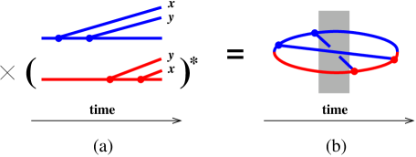
Figure 1: An example of an interference contribution to the rate for (overlapping) sequential splitting, with blue indicating the amplitude and red the conjugate amplitude. In (b), the shading highlights the region of time where the evolution must track four high-energy particles (three in the amplitude and one in the conjugate amplitude).

In more detail, ref. Vqhat discusses how the potential energy for the Schrödinger-like evolution equation can be defined in terms of multi-particle Wilson loops involving lightlike Wilson lines. These are generalizations of the 2-particle Wilson loops that were introduced by Liu, Rajagopal, and Wiedemann LRW1 ; LRW2 as a way to define the medium parameters $\hat{q}_{R}$ for strongly-interacting plasmas. Physically, $\hat{q}_{R}$ characterizes the momentum-space diffusion relation $\langle Q_{\perp}^{2}\rangle=\hat{q}_{R}\,\Delta z$ for the net transverse momentum kick $\bm{Q}_{\perp}$ a high-energy particle picks up from traversing distance $\Delta z$ through the medium, for sufficiently large $\Delta z$. Here, $\hat{q}_{R}$ depends on the color representation $R$ of the high-energy particle (e.g. fundamental representation for quarks and adjoint representation for gluons). In this paper, we start from the result of ref. Vqhat that the multi-particle potentials that are needed for the calculations represented by fig. 1b are harmonic oscillator potentials that can be written in terms of $\hat{q}$ as

$$\underline{V}({\bm{b}}_{1},{\bm{b}}_{2},\cdots,{\bm{b}}_{n})=-\frac{i}{8}\sum_{i>j}(\hat{q}_{i}+\hat{q}_{j}-\underline{\hat{q}_{ij}})({\bm{b}}_{i}{-}{\bm{b}}_{j})^{2}$$ (1)

in the high energy limit, for which the transverse separations of the particles are small. (This high-energy approximation has the same technical caveats, reviewed in ref. Vqhat , as most all other applications of $\hat{q}$.) Above, the ${\bm{b}}_{i}$ are the transverse positions of the high-energy particles during any particular stage of the evolution. $\hat{q}_{i}$ represents the value of $\hat{q}$ for the $i$-th particle. $\hat{q}_{ij}$ represents the value of $\hat{q}$ for the color representation corresponding to the combined color representation of particles $i$ and $j$. In the general case, this combined color representation is not unique. For example, if the $i$ and $j$ represent gluons (which are each in the 8-dimensional adjoint representation of color), then the combination of the two could be any irreducible representation in the SU(3) tensor product $\bm{8}\otimes\bm{8}=\bm{1}\oplus\bm{8}\oplus\bm{8}\oplus\bm{10}\oplus\overline{\bm{10}}\oplus\bm{27}$. Since the values of $\hat{q}$ are mostly different for each irreducible representation, the $\hat{q}_{ij}$ in (1) is not a single number but instead an operator (which can be represented by a finite-dimensional matrix) acting on the color space of the $N$ particles. Following ref. Vqhat , we use underlining to indicate which quantities are color operators in (1).

Ref. Vqhat discusses why the color structure of the $n$-particle potential (1) is trivial for $n{=}3$ because overall color conservation then implies $\underline{\hat{q}_{12}}=\hat{q}_{3}$ and permutations. But the color structure is not trivial for $n{=}4$, which is needed for evolution of the shaded part of fig. 1b.

One main goal of this paper is to find the explicit matrix formula for (1) for the case of four gluons, relevant to the calculation of overlap effects for double bremsstrahlung $g\to ggg$. We will review how there are eight ways to make a color singlet from four gluons. But we will give a symmetry argument that three of those singlets decouple from the color dynamics of $g\to ggg$, leaving us with a 5-dimensional subspace of 4-gluon color singlet states, which mix dynamically due to interactions with the medium. Correspondingly, we will show how $\underline{V}({\bm{b}}_{1},{\bm{b}}_{2},{\bm{b}}_{3},{\bm{b}}_{4})$ is explicitly implemented by a $5{\times}5$ matrix function that is quadratic in transverse separations. We’ll also perform the analysis for SU($N_{\rm c}$) with $N_{\rm c}>3$, to see how potentials previously used in large-$N_{\rm c}$ calculations of overlap effects are recovered as $N_{\rm c}\to\infty$.

With explicit results for the 4-gluon potential in hand, we demonstrate that consistency of the $\hat{q}$ approximation for this application necessarily implies that $\hat{q}$ satisfy Casimir scaling (i.e. $\hat{q}_{R}\propto C_{R}$, where $C_{R}$ is the quadratic Casimir of color representation $R$) for the specific representations relevant to this paper (those generated by $\bm{8}\otimes\bm{8}$). We suspect that Casimir scaling is necessary more generally, but so far we have not pursued a more general argument. Though Casimir scaling of $\hat{q}$ has long been known through next-to-leading order for weakly-coupled plasmas SimonNLO , we are unaware of a previous argument for Casimir scaling in applications to finite-$N_{\rm c}$ strongly-coupled plasmas (again subject to the technical caveats of the $\hat{q}$ approximation reviewed in ref. Vqhat ).

The last goal of this paper is to discuss how to use the explicit potential to calculate overlap effects for $g\to ggg$ in $N_{\rm c}{=}3$ QCD. Though we will write formulas that can in principle be implemented numerically, the practical problem of implementing those numerics will be much more complicated than the case of large-$N_{\rm c}$ QCD, and we do not attempt it today. We will see that the problem involves finding the propagator for a quantum system of two coupled harmonic oscillators whose spring constants are finite-dimensional matrices in a space of additional quantum degrees of freedom:

$$\underline{H}=\frac{p_{1}^{2}}{2m_{1}}+\frac{p_{2}^{2}}{2m_{2}}+\frac{1}{2}\begin{pmatrix}q_{1}\\ q_{2}\end{pmatrix}^{\!\!\top}\begin{pmatrix}\underline{a}&\underline{b}\\ \underline{b}&\underline{c}\end{pmatrix}\begin{pmatrix}q_{1}\\ q_{2}\end{pmatrix},$$ (2)

where here $\underline{a}$, $\underline{b}$, and $\underline{c}$ are constant ($5{\times}5$) symmetric matrices that do not all commute, $q_{1}$ and $q_{2}$ are two positions, $p_{1}$ and $p_{2}$ are the corresponding conjugate momenta, and the “masses” $m_{1}$ and $m_{2}$ are constants (unrelated to actual particle masses, which we ignore). As we’ll discuss, the matrix structure of the spring constants makes computing and using the propagator for the system (2) more difficult for $N_{\rm c}{=}3$ than for the large-$N_{\rm c}$ limit.

Outline

In the next section, we first discuss the different ways that four gluons can make an SU(3) color singlet, and the transformations between different basis choices needed to determine the $\underline{\hat{q}_{ij}}$ in (1) in terms of the values $\hat{q}_{R}$ for different color representations. Explicit transformations may be found in terms of 6-$j$ coefficients taken from the literature NSZ6j ; Zakharov6j ; Sjodahl . We also discuss the permutation symmetries that reduce the 8-dimensional space of singlets to the 5-dimensional subspace relevant for our application.

In section III, we find the 4-body potential in the harmonic approximation (1) by explicitly constructing the matrices $\underline{\hat{q}_{ij}}$. We show that consistency of the color structure of that potential requires that $\hat{q}_{R}$ satisfy Casimir scaling.

In section IV, we briefly review that, for this application, ref. 2brem showed how to use symmetry to reduce the 4-body evolution problem to an effective 2-body evolution problem. We explicitly construct the corresponding harmonic oscillator Hamiltonian, which we will see has the form (2).

Section V discusses the generalization of our analysis to SU($N_{\rm c}$) for $N_{\rm c}{>}3$, which has an interesting twist requiring discussion of how it smoothly matches to $N_{\rm c}{=}3$. We use the SU($N_{\rm c}$) results to see exactly how the color dynamics found in this paper approaches the simpler large-$N_{\rm c}$ results used in previous work on overlapping formation times.

Section VI discusses similarities and differences of this work with earlier work by other authors NSZ6j ; Zakharov6j .

Section VII gives our conclusion, where we discuss the difficulty of matrix-coefficient harmonic oscillator problems like (2) and the prospect for numerics.

In the appendix, we outline our own calculation of SU($N_{\rm c}$) 6-$j$ coefficients involving four gluons.

II Color Singlets and 6-$j$ coefficients for 4 Gluons

II.1 Basics

One way to make a basis of color singlet states from 4 particles (which here we’ll call A, B, C, and D) is depicted in fig. 2a. Consider an irreducible color representation $R$ that appears in both (i) the tensor product $R_{\rm A}\otimes R_{\rm B}$ of the color representations of particles A and B and (ii) the tensor product $R_{\rm C}\otimes R_{\rm D}$ of particles C and D. Combine AB to make $R$ and combine CD to make $R$, and then combine those two $R$’s to make a singlet.

Figure 2: Different ways of making a basis of singlet states for four particles.

There is nothing special about choosing to first make the combinations AB and CD. We could have just as well chosen AC and BD, or AD and BC. We’ll refer to these as $s$-channel, $t$-channel, or $u$-channel choices of bases for the color singlet states, as depicted in figs. 2(a–c) respectively.

The relevant tensor product for combining two gluons is

$$\bm{8}\otimes\bm{8}=\bm{1}_{\rm s}\oplus\bm{8}_{\rm a}\oplus\bm{8}_{\rm s}\oplus\bm{10}_{\rm a}\oplus\overline{\bm{10}}_{\rm a}\oplus\bm{27}_{\rm s},$$ (3)

where the subscripts give the additional information of whether each irreducible representation arises in the symmetric (s) or anti-symmetric (a) combination of $\bm{8}\otimes\bm{8}$. The decomposition (3) means that there are five possibilities ($\bm{1}$, $\bm{8}$, $\bm{10}$, $\overline{\bm{10}}$, and $\bm{27}$) for the $R$ of fig. 2a to obtain color singlets from four gluons. However, there are more than five singlet possibilities because there are two different ways ($\bm{8}_{\rm a}$ and $\bm{8}_{\rm s}$) each pair of gluons (AB or CD) can make an $\bm{8}$, and so there are four different color singlets corresponding to the case $R{=}\bm{8}$ in fig. 2a. Following the notation of ref. Sjodahl , one could denote these four singlets by fig. 3, where a closed circle at a vertex indicates the anti-symmetric combination $\bm{8}_{\rm a}$ of (3) and an open circle represents the symmetric combination $\bm{8}_{\rm s}$. Because of this multiplicity, there are in total eight independent color singlets that can be made from four gluons. The different channels of fig. 2 just provide different ways to choose a basis for the eight-dimensional space of 4-gluon singlets. In what follows, we’ll refer to the $s$-channel basis of the singlet states as

$$|s_{\bm{1}}\rangle,~{}|s_{\bm{8}_{\rm aa}}\rangle,~{}|s_{\bm{8}_{\rm as}}\rangle,~{}|s_{\bm{8}_{\rm sa}}\rangle,~{}|s_{\bm{8}_{\rm aa}}\rangle,~{}|s_{\bm{10}}\rangle,~{}|s_{\overline{\bm{10}}}\rangle,~{}|s_{\bm{27}}\rangle,$$ (4)

and similarly for the corresponding $t$-channel or $u$-channel bases.

Figure 3: Different ways to make the $R{=}\bm{8}$ case of fig. 2a. Closed and open circles represent the anti-symmetric and symmetric combinations $\bm{8}_{\rm a}$ and $\bm{8}_{\rm s}$, respectively.

The 4-gluon case of the potential (1) is

$$\underline{V}({\bm{b}}_{1},{\bm{b}}_{2},{\bm{b}}_{3},{\bm{b}}_{4})=-\frac{i}{8}\Bigl{\{} (2\hat{q}_{{\rm Adj}}-\underline{\hat{q}_{12}})\bigl{[}({\bm{b}}_{1}{-}{\bm{b}}_{2})^{2}+({\bm{b}}_{3}{-}{\bm{b}}_{4})^{2}\bigr{]}$$

$$+(2\hat{q}_{{\rm Adj}}-\underline{\hat{q}_{13}})\bigl{[}({\bm{b}}_{1}{-}{\bm{b}}_{3})^{2}+({\bm{b}}_{2}{-}{\bm{b}}_{4})^{2}\bigr{]}$$

$$+(2\hat{q}_{{\rm Adj}}-\underline{\hat{q}_{14}})\bigl{[}({\bm{b}}_{1}{-}{\bm{b}}_{4})^{2}+({\bm{b}}_{2}{-}{\bm{b}}_{3})^{2}\bigr{]}\Bigr{\}},$$ (5)

where “${\rm Adj}$” means adjoint representation. Let the particle labels $1,2,3,4$ here correspond to the $A,B,C,D$ of fig. 2. Then the $s$-channel basis (4) diagonalizes $\underline{\hat{q}_{12}}$, since the $R$ in fig. 2a is the joint color representation of the first two particles. In the $s$-channel basis (4),

$$\underline{\hat{q}_{12}}=\underline{\hat{q}}_{\rm diag}\equiv\begin{pmatrix}\,0\,&&&&&&&\\ &\hat{q}_{{\rm Adj}}&&&&&&\\ &&\hat{q}_{{\rm Adj}}&&&&&\\ &&&\hat{q}_{{\rm Adj}}&&&&\\ &&&&\hat{q}_{{\rm Adj}}&&&\\ &&&&&\hat{q}_{\bm{10}}&&\\ &&&&&&\hat{q}_{\bm{10}}&\\ &&&&&&&\hat{q}_{\bm{27}}\end{pmatrix}.$$ (6)

Similarly, the $t$-channel basis diagonalizes $\underline{\hat{q}_{13}}$, and the $u$-channel basis diagonalizes $\underline{\hat{q}_{14}}$. In order to express the potential (5) explicitly in a single choice of basis, we need to know how to convert between these bases choices. We will choose to express the potential in the $s$-channel basis, and so we need the unitary matrices $\underline{\langle s|t\rangle}$ and $\underline{\langle s|u\rangle}$ of normalized overlaps

$$\langle s_{i}|t_{j}\rangle\qquad\mbox{and}\qquad\langle s_{i}|u_{j}\rangle$$ (7)

to construct

$$\underline{\hat{q}_{13}}=\underline{\langle s|t\rangle}\,\underline{\hat{q}}_{\rm diag}\,\underline{\langle s|t\rangle}^{\dagger},\qquad\underline{\hat{q}_{14}}=\underline{\langle s|u\rangle}\,\underline{\hat{q}}_{\rm diag}\,\underline{\langle s|u\rangle}^{\dagger}$$ (8)

in that basis. Up to normalization and sign conventions, the overlaps (7) are the QCD 6-$j$ coefficients, which can be represented diagrammatically as in fig. 4, or as a QCD version

$$\left\{\begin{matrix}{\rm Adj}&{\rm Adj}&{\cal R}\\ {\rm Adj}&{\rm Adj}&{\cal R^{\prime}}\end{matrix}\right\}$$ (9)

of the Wigner 6-$j$ symbols

$$\left\{\begin{matrix}j_{1}&j_{2}&J\\ j_{3}&j_{4}&J^{\prime}\end{matrix}\right\}$$ (10)

for angular momentum. [In the case where the combined color representation $R$ or $R^{\prime}$ of a pair of gluons is an $\bm{8}$, then the ${\cal R}$ or ${\cal R}^{\prime}$ in (9) must also contain the information of whether that $\bm{8}$ couples as the $\bm{8}_{\rm aa}$, $\bm{8}_{\rm as}$, $\bm{8}_{\rm sa}$ or $\bm{8}_{\rm ss}$ cases of fig. 3.]

Figure 4: A diagram representing (up to normalization and sign conventions) the overlap $\langle s_{\cal R}|t_{{\cal R}^{\prime}}\rangle$, where solid lines represent the adjoint representations for each of our 4 gluons. [It also represents the overlap $\langle s_{\cal R}|u_{{\cal R}^{\prime}}\rangle$, depending on how the 4 solid lines are identified with the particles ABCD of fig. 2.] When supplemented as necessary by the filled or open circles of fig. 3 in the case that ${\cal R}$ or ${\cal R}^{\prime}$ is an adjoint representation, these diagrams are equivalent to those appearing in ref. Sjodahl . The arrows shown above for ${\cal R}$ and ${\cal R}^{\prime}$ are only relevant to the convention for distinguishing $\bf{10}$ vs. $\overline{\bf{10}}$ or $\bm{8}_{as}$ vs. $\bm{8}_{sa}$ in this diagram when comparing to ref. Sjodahl .

For SU(3), the values of these overlaps can be extracted from refs. NSZ6j ; Zakharov6j or Sjodahl . The values of $\langle s_{i}|t_{j}\rangle$ for conventionally normalized states $|s_{i}\rangle$ and $|t_{j}\rangle$, which gives the unitary transformation between the $t$-channel and $s$-channel bases for 4-gluon singlets, is shown in table 1. [We have also verified these overlaps independently, which we briefly summarize in appendix A for the sake of convenient reference.]

$\langle s_{\cal R}|t_{{\cal R}^{\prime}}\rangle$	$\bm{1}$	$\bm{8}_{\rm aa}$	$\bm{8}_{\rm as}$	$\bm{8}_{\rm sa}$	$\bm{8}_{\rm ss}$	$\bm{10}$	$\overline{\bm{10}}$	$\bm{27}$	conversion to $\langle s_{\cal R}|u_{{\cal R}^{\prime}}\rangle$
$\bm{1}$	$\frac{1}{8}$	$\frac{1}{2\sqrt{2}}$	$0$	$0$	$\frac{1}{2\sqrt{2}}$	$\frac{\sqrt{5}}{4\sqrt{2}}$	$\frac{\sqrt{5}}{4\sqrt{2}}$	$\frac{3\sqrt{3}}{8}$	$+$
$\bm{8}_{\rm aa}$	$\frac{1}{2\sqrt{2}}$	$\frac{1}{2}$	$0$	$0$	$\frac{1}{2}$	$0$	$0$	$-\frac{\sqrt{3}}{2\sqrt{2}}$	$-$
$\bm{8}_{\rm as}$	$0$	$0$	$-\frac{1}{2}$	$\frac{1}{2}$	$0$	$-\frac{1}{2}$	$\frac{1}{2}$	$0$	$+$
$\bm{8}_{\rm sa}$	$0$	$0$	$\frac{1}{2}$	$-\frac{1}{2}$	$0$	$-\frac{1}{2}$	$\frac{1}{2}$	$0$	$-$
$\bm{8}_{\rm ss}$	$\frac{1}{2\sqrt{2}}$	$\frac{1}{2}$	$0$	$0$	$-\frac{3}{10}$	$-\frac{1}{\sqrt{5}}$	$-\frac{1}{\sqrt{5}}$	$\frac{3\sqrt{3}}{10\sqrt{2}}$	$+$
$\bm{10}$	$\frac{\sqrt{5}}{4\sqrt{2}}$	$0$	$-\frac{1}{2}$	$-\frac{1}{2}$	$-\frac{1}{\sqrt{5}}$	$\frac{1}{4}$	$\frac{1}{4}$	$-\frac{\sqrt{3}}{4\sqrt{10}}$	$-$
$\overline{\bm{10}}$	$\frac{\sqrt{5}}{4\sqrt{2}}$	$0$	$\frac{1}{2}$	$\frac{1}{2}$	$-\frac{1}{\sqrt{5}}$	$\frac{1}{4}$	$\frac{1}{4}$	$-\frac{\sqrt{3}}{4\sqrt{10}}$	$-$
$\bm{27}$	$\frac{3\sqrt{3}}{8}$	$-\frac{\sqrt{3}}{2\sqrt{2}}$	$0$	$0$	$\frac{3\sqrt{3}}{10\sqrt{2}}$	$-\frac{\sqrt{3}}{4\sqrt{10}}$	$-\frac{\sqrt{3}}{4\sqrt{10}}$	$\frac{7}{40}$	$+$

Table 1: Normalized $st$-channel overlaps $\langle s_{\cal R}|t_{{\cal R}^{\prime}}\rangle$ of SU(3) singlets of four adjoint particles, where row labels indicate ${\cal R}$ and column labels indicate ${\cal R}^{\prime}$. Conversion to the corresponding $su$-channel overlaps $\langle s_{\cal R}|u_{{\cal R}^{\prime}}\rangle$ is given by multiplying each row of $\langle s|t\rangle$ by the sign shown in the last column above.

We should note that changing sign convention for the normalization of a basis state $|s_{\cal R}\rangle$ would negate the corresponding row of table 1, and a similar change of sign convention for a $|t_{{\cal R}^{\prime}}\rangle$ would negate the corresponding column. So table 1 corresponds to a specific choice of sign conventions for the definition of the basis states.

The coefficients $\langle s_{\cal R}|u_{{\cal R^{\prime}}}\rangle$ giving the transformation from the $u$-basis to the $s$-basis may now be obtained by swapping the labeling of particles C and D in fig. 2 to interchange $t$ channel with $u$ channel. Specifically, we’ll define our $u$ channel singlet states (including sign convention) by

$$|u_{\cal R}\rangle\equiv|t_{\cal R}\rangle~{}\mbox{with C$\leftrightarrow$D}.$$ (11)

Then

$$\langle s_{\cal R}|u_{{\cal R}^{\prime}}\rangle=\langle s_{\cal R}|\Bigl{(}|t_{{\cal R}^{\prime}}\rangle~{}\mbox{with C$\leftrightarrow$D}\Bigr{)}=\Bigl{(}\langle s_{\cal R}|~{}\mbox{with C$\leftrightarrow$D}\Bigr{)}|t_{{\cal R}^{\prime}}\rangle.$$ (12)

This corresponds to constructing $\underline{\langle s|u\rangle}$ from $\underline{\langle s|t\rangle}$ by negating those rows of table 1 where $C$ and $D$ are combined anti-symmetrically in $|s_{\cal R}\rangle$. According to (3), that’s ${\cal R}=\bm{8}_{\rm aa}$, $\bm{8}_{\rm sa}$, $\bm{10}$ and $\overline{\bm{10}}$. We show the signs corresponding to this conversion in the last column of table 1.

II.2 Block Diagonalization with Permutation Symmetries

Because the four representations we are combining into singlets are identical (four adjoints), there are certain permutation symmetries of ABCD that can be used to simultaneously block-diagonalize $\underline{\langle s|t\rangle}$ and $\underline{\langle s|u\rangle}$ and so reduce the number of singlet states that need be considered. Specifically, consider the channel-preserving permutations of ABCD that simultaneously map $s$-channel to $s$-channel, $t$-channel to $t$-channel, and $u$-channel to $u$-channel. From fig. 2, these are the symmetries of the rectangle one could draw connecting the labels ABCD shown in each of those diagrams. That is, there are two reflection symmetries

$$\sigma_{1}:~{}ABCD\leftrightarrow BADC,\qquad\sigma_{2}:~{}ABCD\leftrightarrow CDAB,$$ (13a)

and the $$180^{\circ}$$ rotation symmetry

$$\sigma_{3}:~{}ABCD\leftrightarrow DCBA.$$ (13b)

The symmetry group of the rectangle (known as $D_{2}$) is equivalent to $Z_{2}\otimes Z_{2}$, where any two of the three symmetries (13) may be thought of as the two generators. In each channel, it will be useful to choose a new basis for our singlet states, having definite charge $(\sigma_{1},\sigma_{2},\sigma_{3})=(\pm_{1},\pm_{2},\pm_{3})$ under all three symmetries (13). That’s slightly redundant, since $\sigma_{1}\sigma_{2}\sigma_{3}$ is the identity transformation and so $\sigma_{1}\sigma_{2}\sigma_{3}=+1$. But the redundancy is useful for seeing a simple relation between charges in different channels: Consider $ABCD\rightarrow ACBD$, which changes $s$-channel to $t$-channel, and similarly $ABCD\rightarrow ADBC$ for $s$-channel to $u$-channel. Their actions on (13) give

$$\mbox{ $(\sigma_{1},\sigma_{2},\sigma_{3})=(\sigma_{1}^{s},\sigma_{2}^{s},\sigma_{3}^{s})$ in $s$-channel construction }\\ \longrightarrow\begin{cases}\mbox{ $(\sigma_{1},\sigma_{2},\sigma_{3})=(\sigma_{2}^{s},\sigma_{1}^{s},\sigma_{3}^{s})$ in $t$-channel construction; }\\ \mbox{ $(\sigma_{1},\sigma_{2},\sigma_{3})=(\sigma_{2}^{s},\sigma_{3}^{s},\sigma_{1}^{s})$ in $u$-channel construction. }\end{cases}$$ (14)

For each channel, table 2 lists ($\sigma_{1},\sigma_{2},\sigma_{3})$ eigenstates and values.

singlet state	$(\sigma_{1},\sigma_{2},\sigma_{3})$
(channel ${\rm ch}=s$, $t$, or $u$)	$s$-channel	$t$-channel	$u$-channel
$|{\rm ch}_{\bm{1}}\rangle$	$(+,+,+)$	$(+,+,+)$	$(+,+,+)$
$|{\rm ch}_{\bm{8}_{\rm aa}}\rangle$
$|{\rm ch}_{\bm{8}_{\rm ss}}\rangle$
$\tfrac{1}{\sqrt{2}}\bigl{(}|{\rm ch}_{\bm{10}}\rangle+|{\rm ch}_{\overline{\bm{10}}}\rangle\bigr{)}$
$|{\rm ch}_{\bm{27}}\rangle$
$\tfrac{1}{\sqrt{2}}\bigl{(}|{\rm ch}_{\bm{8}_{\rm as}}\rangle+|{\rm ch}_{\bm{8}_{\rm sa}}\rangle\bigr{)}$	$(-,+,-)$	$(+,-,-)$	$(+,-,-)$
$\tfrac{1}{\sqrt{2}}\bigl{(}|{\rm ch}_{\bm{8}_{\rm as}}\rangle-|{\rm ch}_{\bm{8}_{\rm sa}}\rangle\bigr{)}$	$(-,-,+)$	$(-,-,+)$	$(-,+,-)$
$\tfrac{1}{\sqrt{2}}\bigl{(}|{\rm ch}_{\bm{10}}\rangle-|{\rm ch}_{\overline{\bm{10}}}\rangle\bigr{)}$	$(+,-,-)$	$(-,+,-)$	$(-,-,+)$

Table 2: For each channel, the signs $(\sigma_{1},\sigma_{2},\sigma_{3})$ of the singlet states under the three channel-preserving permutations $(ABCD{\leftrightarrow}BADC,ABCD{\leftrightarrow}CDBA,ABCD{\leftrightarrow}DCBA)$.

Two states $|s_{\cal R}\rangle$ and $|t_{\cal R^{\prime}}\rangle$ must have zero overlap $\langle s_{\cal R}|t_{\cal R^{\prime}}\rangle$ if their charges $(\sigma_{1},\sigma_{2},\sigma_{3})$ are different, and similarly for $|s_{\cal R}\rangle$, $|u_{\cal R^{\prime}}\rangle$, and $\langle s_{\cal R}|u_{\cal R^{\prime}}\rangle$. That means that the first five rows of table 2 do not mix with the last three rows, when one considers combining interactions mediated by different channels. Specifically, the forms (6) and (8) of $\underline{\hat{q}_{12}}$, $\underline{\hat{q}_{13}}$, and $\underline{\hat{q}_{14}}$ then imply that the 4-particle potential (5) block diagonalizes into $5{\times}5$ and $3{\times}3$ blocks corresponding to the first five rows and last three rows of table 2. We will now see that our application lies within the $5{\times}5$ block, and so we may ignore the $3{\times}3$ block.

II.3 Our application is a $5{\times}5$ problem

Consider an interference diagram such as fig. 1b for $g\to ggg$, which we used to introduce the need for the 4-gluon potential. We show the diagram again in fig. 5, now with the adjoint color indices of the gluons labeled, and with the regions of 3-particle evolution shaded in light blue (in addition to the 4-particle evolution shaded in gray). The important point about this diagram, true of any interference diagram for $g\to ggg$, is that 3-gluon vertices are associated with color factors given by Lie algebra structure constants $f_{abc}$. In consequence, the three gluons during the first phase of evolution are in the color singlet state

$$f_{CDe}|CDe\rangle.$$ (15)

None of the interactions with the medium can change this (after medium averaging), and so the color state remains the same just before the second vertex in fig. 5. That vertex then splits $e$ into $AB$ with a color factor of $f_{ABe}$, which means the intermediate (gray-shaded) region of 4-gluon evolution starts in color state

$$f_{ABe}f_{CDe}|ABCD\rangle.$$ (16)

This corresponds to particles AB being combined anti-symmetrically into a color adjoint state $f_{ABe}|AB\rangle$ and particles CD being similarly combined anti-symmetrically into a color adjoint state $f_{CDe}|CD\rangle$, and then an overall 4-gluon color singlet made from combining the two pairs. That is, the initial state (16) for 4-gluon evolution is (once normalized) just what we’ve been calling $|s_{\bm{8}_{\rm aa}}\rangle$ in this paper. That places the 4-gluon evolution into the 5-dimensional subspace given by the first 5 rows of table 2.

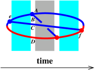
Figure 5: Similar to fig. 1 but here showing labels for the adjoint color indices of all gluon lines.

A similar argument working backward from the latest time in fig. 5 shows that the end color state of the 4-gluon evolution should be taken to be

$$|t_{\bm{8}_{\rm aa}}\rangle\propto f_{ACe}f_{BDe}|ABCD\rangle.$$ (17)

Which channel the end 4-gluon state is in compared to the initial 4-gluon state depends on the interference diagram. For example, for diagrams like fig. 6, both will be $|s_{\bm{8}_{\rm aa}}\rangle$. Regardless, everything will be in the sector of $(\sigma_{1},\sigma_{2},\sigma_{3}){=}(+,+,+)$ singlet states.

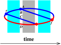
Figure 6: Similar to fig. 5 but for a different $g\to ggg$ interference diagram.

The $5{\times}5$ unitary matrix of $\langle s|t\rangle$ overlaps in the $(\sigma_{1},\sigma_{2},\sigma_{3}){=}(+,+,+)$ subspace is shown explicitly in table 3.

$\langle s_{\cal R}|t_{{\cal R}^{\prime}}\rangle$	$\bm{1}$	$\bm{8}_{\rm aa}$	$\bm{8}_{\rm ss}$	$\bm{10}{+}\overline{\bm{10}}$	$\bm{27}$	conversion to $\langle s_{\cal R}|u_{{\cal R}^{\prime}}\rangle$
$\bm{1}$	$\frac{1}{8}$	$\frac{1}{2\sqrt{2}}$	$\frac{1}{2\sqrt{2}}$	$\frac{\sqrt{5}}{4}$	$\frac{3\sqrt{3}}{8}$	$+$
$\bm{8}_{\rm aa}$	$\frac{1}{2\sqrt{2}}$	$\frac{1}{2}$	$\frac{1}{2}$	$0$	$-\frac{\sqrt{3}}{2\sqrt{2}}$	$-$
$\bm{8}_{\rm ss}$	$\frac{1}{2\sqrt{2}}$	$\frac{1}{2}$	$-\frac{3}{10}$	$-\frac{\sqrt{2}}{\sqrt{5}}$	$\frac{3\sqrt{3}}{10\sqrt{2}}$	$+$
$\bm{10}{+}\overline{\bm{10}}$	$\frac{\sqrt{5}}{4}$	$0$	$-\frac{\sqrt{2}}{\sqrt{5}}$	$\frac{1}{2}$	$-\frac{\sqrt{3}}{4\sqrt{5}}$	$-$
$\bm{27}$	$\frac{3\sqrt{3}}{8}$	$-\frac{\sqrt{3}}{2\sqrt{2}}$	$\frac{3\sqrt{3}}{10\sqrt{2}}$	$-\frac{\sqrt{3}}{4\sqrt{5}}$	$\frac{7}{40}$	$+$

Table 3: Normalized $st$-channel overlaps $\langle s_{\cal R}|t_{{\cal R}^{\prime}}\rangle$ for the relevant subspace of SU(3) singlets of four adjoint particles. Here $\bm{10}{+}\overline{\bm{10}}$ is shorthand for the $\tfrac{1}{\sqrt{2}}\bigl{(}|{\rm ch}_{\bm{10}}\rangle+|{\rm ch}_{\overline{\bm{10}}}\rangle\bigr{)}$ state of table 2. The last column shows how to convert to $\langle s_{\cal R}|u_{{\cal R}^{\prime}}\rangle$ just as in table 1.

III The explicit potential and Casimir scaling

III.1 The 4-body potential

Restricting attention to the $5$-dimensional subspace of relevant singlets, the 4-gluon potential is now given by (5) with

$$\underline{\hat{q}_{12}}=\underline{\hat{q}}_{\rm diag}\equiv\begin{pmatrix}\,0\,&&&&\\ &\hat{q}_{{\rm Adj}}&&&\\ &&\hat{q}_{{\rm Adj}}&&\\ &&&\hat{q}_{\bm{10}}&\\ &&&&\hat{q}_{\bm{27}}\end{pmatrix},$$ (18a)

$$\underline{\hat{q}_{13}}=\underline{\langle s|t\rangle}\,\underline{\hat{q}}_{\rm diag}\,\underline{\langle s|t\rangle}^{\dagger},$$ (18b)

and

$$\underline{\hat{q}_{14}}=\underline{\langle s|u\rangle}\,\underline{\hat{q}}_{\rm diag}\,\underline{\langle s|u\rangle}^{\dagger}=\underline{P}\,\underline{\hat{q}_{13}}\,\underline{P},$$ (18c)

where $$\underline{\langle s|t\rangle} \underline{P}$$ is given by table 3, and is a diagonal matrix composed of the signs in the last column of that table:

$$\underline{P}\equiv\begin{pmatrix}$+$&&&&\\ &$-$&&&\\ &&$+$&&\\ &&&$-$&\\ &&&&$+$\end{pmatrix}.$$ (18d)

III.2 An additional consistency condition

Ref. Vqhat showed that consistency of the harmonic oscillator ($\hat{q}$) approximation to the $n$-body potential requires that approximation to have the form (1) and so, in the 4-body case, requires (5). However, ref. Vqhat did not show the inverse: it did not prove that (1) is always consistent. “Consistency” here means that the $n$-body potential matches the $(n{-}1)$-body potential in the special cases where two of the particles are in the same place (i.e. ${\bm{b}}_{i}{=}{\bm{b}}_{j}$ for some $i$ and $j$). We’re now in a position to check this for the 4-gluon potential given by (5), (18), and table 3. Consider the special case where ${\bm{b}}_{3}{=}{\bm{b}}_{4}$ in (5), giving

$$\underline{V}({\bm{b}}_{1},{\bm{b}}_{2},{\bm{b}}_{3},{\bm{b}}_{3})=-\frac{i}{8}\Bigl{\{}(2\hat{q}_{{\rm Adj}}-\underline{\hat{q}_{12}})({\bm{b}}_{1}{-}{\bm{b}}_{2})^{2}+(4\hat{q}_{{\rm Adj}}-\underline{\hat{q}_{13}}-\underline{\hat{q}_{14}})\bigl{[}({\bm{b}}_{1}{-}{\bm{b}}_{3})^{2}+({\bm{b}}_{2}{-}{\bm{b}}_{3})^{2}\bigr{]}\Bigr{\}}.$$ (19)

However, as in ref. Vqhat , we may alternatively think of this situation as a three-particle problem by replacing coincident particles 3 and 4 above by a single particle with their combined color representation, i.e. by replacing $\hat{q}_{3}\to\underline{\hat{q}_{34}}$ in the formula for a 3-body particles potential.

Generically, the 3-body case of the $n$-body potential (1) is Vqhat ; 2brem

$$\underline{V}({\bm{b}}_{1},{\bm{b}}_{2},{\bm{b}}_{3})=-\frac{i}{8}\Bigl{\{}(\hat{q}_{1}+\hat{q}_{2}-\hat{q}_{3})({\bm{b}}_{1}{-}{\bm{b}}_{2})^{2}+(\hat{q}_{2}+\hat{q}_{3}-\hat{q}_{1})({\bm{b}}_{2}{-}{\bm{b}}_{3})^{2}+(\hat{q}_{3}+\hat{q}_{1}-\hat{q}_{2})({\bm{b}}_{3}{-}{\bm{b}}_{1})^{2}\Bigr{\}},$$ (20)

where the fact that the potential is for an overall 3-body color singlet has been used to replace the $\underline{\hat{q}_{12}}$ of (1) by $\hat{q}_{3}$ in (20), with similar replacements for $\underline{\hat{q}_{13}}$ and $\underline{\hat{q}_{23}}$. Consistency of (19) and (20) then implies that we must have

$$\underline{V}({\bm{b}}_{1},{\bm{b}}_{2},{\bm{b}}_{3},{\bm{b}}_{3})=\Bigl{[}V({\bm{b}}_{1},{\bm{b}}_{2},{\bm{b}}_{3})~{}\mbox{with $\hat{q}_{3}\to\underline{\hat{q}_{34}}$}\Bigr{]}.$$ (21)

Ref. Vqhat focused on the consistency of what, in the case of (19), would be the $({\bm{b}}_{1}{-}{\bm{b}}_{2})^{2}$ term. Appropriately generalized, that comparison was the basis for how the $n$-body potential (1) was determined. Here, let’s also check the consistency of the other terms in (19). Comparing (19) to (20) via (21), we see that full consistency of the 4-gluon potential is achieved if and only if additionally

$$4\hat{q}_{\rm Adj}-\underline{\hat{q}_{13}}-\underline{\hat{q}_{14}}=\underline{\hat{q}_{34}}.$$ (22)

$\underline{\hat{q}_{34}}=\underline{\hat{q}_{12}}$ since the 4 gluons form a color singlet, and so we can rewrite the consistency condition (22) as

$$\underline{\hat{q}_{12}}+\underline{\hat{q}_{13}}+\underline{\hat{q}_{14}}=4\hat{q}_{\rm Adj}.$$ (23)

This same condition could alternatively be derived by looking at the special case ${\bm{b}}_{2}{=}{\bm{b}}_{3}{=}{\bm{b}}_{4}$ of the 4-gluon potential (5),

$$\underline{V}({\bm{b}}_{1},{\bm{b}}_{2},{\bm{b}}_{2},{\bm{b}}_{2})=-\frac{i}{8}(6\hat{q}_{{\rm Adj}}-\underline{\hat{q}_{12}}-\underline{\hat{q}_{13}}-\underline{\hat{q}_{14}})({\bm{b}}_{1}{-}{\bm{b}}_{2})^{2}\Bigr{\}}.$$ (24)

By overall color neutrality, the combination of the coincident particles 2, 3, and 4 must be in the adjoint representation, and so (24) must match up with the 2-gluon potential $V({\bm{b}}_{1},{\bm{b}}_{2})=-\frac{i}{8}(2\hat{q}_{\rm Adj})({\bm{b}}_{1}-{\bm{b}}_{2})^{2}$. That matching also gives (23).

III.3 Consistency implies Casimir Scaling of $\hat{q}$

Using the explicit formulas of (18) and table 3, we find that (23) is satisfied only if the $\hat{q}_{R}$ for the three non-trivial representations $R=\bm{8}$, $\bm{10}$, and $\bm{27}$ appearing in our analysis are related by Casimir scaling. Namely, consistency requires

$$\hat{q}_{\bm{10}}=\frac{C_{\bm{10}}}{C_{\rm Adj}}\,\hat{q}_{\rm Adj}=2\hat{q}_{\rm Adj}\quad\mbox{and}\quad\hat{q}_{\bm{27}}=\frac{C_{\bm{27}}}{C_{\rm Adj}}\,\hat{q}_{\rm Adj}=\tfrac{8}{3}\hat{q}_{\rm Adj}.$$ (25)

We speculate that there is a general argument that applies to other representations as well, but in this paper we focus only on the application to 4-gluon potentials.

Casimir scaling implies that

$$\underline{\hat{q}_{ij}}=\frac{\underline{C_{ij}}}{C_{\rm Adj}}\,\hat{q}_{\rm Adj}=\frac{(\underline{{\mathbb{T}}}_{i}+\underline{{\mathbb{T}}}_{j})^{2}}{C_{\rm Adj}}\,\hat{q}_{\rm Adj}=\frac{C_{i}+2\underline{{\mathbb{T}}}_{i}\cdot\underline{{\mathbb{T}}}_{j}+C_{j}}{C_{\rm Adj}}\,\hat{q}_{\rm Adj},$$ (26)

where (following the notation of ref. Vqhat ) $\underline{{\mathbb{T}}}_{i}^{a}$ are the color generators acting on particle $i$, and $\underline{{\mathbb{T}}}_{i}\cdot\underline{{\mathbb{T}}}_{j}\equiv\underline{{\mathbb{T}}}^{a}_{i}\cdot\underline{{\mathbb{T}}}^{a}_{j}$. The 4-gluon potential (5) can then be rewritten as

$$\underline{V}({\bm{b}}_{1},{\bm{b}}_{2},{\bm{b}}_{3},{\bm{b}}_{4})=\frac{i\hat{q}_{\rm Adj}}{4}\biggl{\{} \frac{\underline{{\mathbb{T}}}_{1}\cdot\underline{{\mathbb{T}}}_{2}}{C_{\rm Adj}}\bigl{[}({\bm{b}}_{1}{-}{\bm{b}}_{2})^{2}+({\bm{b}}_{3}{-}{\bm{b}}_{4})^{2}\bigr{]}$$

$$+\frac{\underline{{\mathbb{T}}}_{1}\cdot\underline{{\mathbb{T}}}_{3}}{C_{\rm Adj}}\bigl{[}({\bm{b}}_{1}{-}{\bm{b}}_{3})^{2}+({\bm{b}}_{2}{-}{\bm{b}}_{4})^{2}\bigr{]}$$

$$+\frac{\underline{{\mathbb{T}}}_{1}\cdot\underline{{\mathbb{T}}}_{4}}{C_{\rm Adj}}\bigl{[}({\bm{b}}_{1}{-}{\bm{b}}_{4})^{2}+({\bm{b}}_{2}{-}{\bm{b}}_{3})^{2}\bigr{]}\biggr{\}},$$ (27)

which has the same form as the weakly-coupled plasma result discussed in Vqhat but here is now a feature for $\hat{q}$ approximations in strongly-coupled plasmas as well.

We can relate the ${{\mathbb{T}}}_{i}\cdot{{\mathbb{T}}}_{j}$ of (27) back to (18) for the $\underline{\hat{q}_{ij}}$ via

$$\frac{\underline{{\mathbb{T}}}_{i}\cdot\underline{{\mathbb{T}}}_{j}}{C_{\rm Adj}}=\frac{\underline{\hat{q}_{ij}}}{2\hat{q}_{\rm Adj}}-\underline{\mathds{1}}.$$ (28)

This yields explicit results

$$\frac{\underline{{\mathbb{T}}}_{1}\cdot\underline{{\mathbb{T}}}_{2}}{C_{\rm Adj}}=-\underline{S}\,,\qquad\frac{\underline{{\mathbb{T}}}_{1}\cdot\underline{{\mathbb{T}}}_{3}}{C_{\rm Adj}}=\tfrac{1}{2}(\underline{S}-\underline{\mathds{1}})-\underline{T}\,,\qquad\frac{\underline{{\mathbb{T}}}_{1}\cdot\underline{{\mathbb{T}}}_{4}}{C_{\rm Adj}}=\tfrac{1}{2}(\underline{S}-\underline{\mathds{1}})+\underline{T}\,,$$ (29a)

where

$$\underline{S}\equiv\begin{pmatrix}~{}1&&&&\\ &~{}\tfrac{1}{2}&&&\\ &&~{}\tfrac{1}{2}&&\\ &&&~{}0&\\ &&&&-\tfrac{1}{3}\end{pmatrix},\qquad\underline{T}\equiv\begin{pmatrix}0&\tfrac{1}{2\sqrt{2}}&0&0&0\\ \frac{1}{2\sqrt{2}}&0&\tfrac{1}{4}&0&\tfrac{1}{2\sqrt{6}}\\ 0&\tfrac{1}{4}&0&\tfrac{1}{\sqrt{10}}&0\\ 0&0&\tfrac{1}{\sqrt{10}}&0&\tfrac{1}{\sqrt{15}}\\ 0&\tfrac{1}{2\sqrt{6}}&0&\tfrac{1}{\sqrt{15}}&0\end{pmatrix}.$$ (29b)

IV Reduction of 4-body to effective 2-body problem

For applications to overlapping formation times, ref. 2brem showed that symmetries and conservation laws could be used to mathematically reduce the 4-body evolution problem to an effective 2-body evolution problem. In the notation of ref. 2brem , we can rewrite differences of $({\bm{b}}_{1},{\bm{b}}_{2},{\bm{b}}_{3},{\bm{b}}_{4})$ in terms of $({\bm{{\cal C}}}_{12},{\bm{{\cal C}}}_{34})$ with

$${\bm{{\cal C}}}_{ij}\equiv\frac{{\bm{b}}_{i}{-}{\bm{b}}_{j}}{x_{i}{+}x_{j}},$$ (30)

where $x_{i}$ is the longitudinal momentum fraction of particle $i$ in figs. 5 or 6, relative to the longitudinal momentum of the initial gluon that started the $g\to ggg$ double splitting process. The $x_{i}$ are defined with a sign convention for particles in the conjugate amplitude so that $x_{1}+x_{2}+x_{3}+x_{4}=0$. The relations are

$${\bm{b}}_{1}-{\bm{b}}_{2} =(x_{1}+x_{2}){\bm{{\cal C}}}_{12},$$ (31a)

$${\bm{b}}_{1}-{\bm{b}}_{3} =x_{2}{\bm{{\cal C}}}_{12}-x_{4}{\bm{{\cal C}}}_{34},$$ (31b)

$${\bm{b}}_{1}-{\bm{b}}_{4} =x_{2}{\bm{{\cal C}}}_{12}+x_{3}{\bm{{\cal C}}}_{34},$$ (31c)

$${\bm{b}}_{2}-{\bm{b}}_{3} =-x_{1}{\bm{{\cal C}}}_{12}-x_{4}{\bm{{\cal C}}}_{34},$$ (31d)

$${\bm{b}}_{2}-{\bm{b}}_{4} =-x_{1}{\bm{{\cal C}}}_{12}+x_{3}{\bm{{\cal C}}}_{34},$$ (31e)

$${\bm{b}}_{3}-{\bm{b}}_{4} =(x_{3}+x_{4}){\bm{{\cal C}}}_{34}.$$ (31f)

Eqs. (27) and (29a) then give

$$\underline{V}({\bm{{\cal C}}}_{12},{\bm{{\cal C}}}_{34})=-\tfrac{i}{4}\hat{q}_{\rm Adj}\Bigl{\{}(x_{1}^{2}+2x_{1}x_{2}\underline{S}+x_{2}^{2}){\cal C}_{12}^{2}+(x_{3}^{2}+2x_{3}x_{4}\underline{S}+x_{4}^{2}){\cal C}_{34}^{2}\\ +2\bigl{[}\tfrac{1}{2}(x_{1}-x_{2})(x_{3}-x_{4})(\underline{S}-1)-(x_{1}+x_{2})(x_{3}+x_{4})\underline{T}\bigr{]}{\bm{{\cal C}}}_{12}\cdot{\bm{{\cal C}}}_{34}\Bigr{\}}.$$ (32a)

Ref. 2brem shows that the Schrödinger-like problem describing 4-particle evolution has Hamiltonian

$$\underline{H}=\frac{P_{12}^{2}}{2x_{1}x_{2}(x_{1}{+}x_{2})E}+\frac{P_{34}^{2}}{2x_{3}x_{4}(x_{3}{+}x_{4})E}+\underline{V}({\bm{{\cal C}}}_{12},{\bm{{\cal C}}}_{34}),$$ (32b)

except that the potential $V({\bm{{\cal C}}}_{12},{\bm{{\cal C}}}_{34})$ there has been replaced by a $5{\times}5$ matrix-valued potential here, as indicated by the underlining above. ${\bm{P}}_{12}$ and ${\bm{P}}_{34}$ are the momenta conjugate to ${\bm{{\cal C}}}_{12}$ and ${\bm{{\cal C}}}_{34}$, and $E$ is the energy of the initial gluon in the $g\to ggg$ double splitting process.

The Hamiltonian (32b) is of the form (2) previewed in the introduction except that the position variables $q_{1}$ and $q_{2}$ are two-dimensional transverse position vectors ${\bm{{\cal C}}}_{12}$ and ${\bm{{\cal C}}}_{34}$. So (2) is more explicitly of the form

$$\underline{H}=\sum_{i=x,y}\left[\frac{p_{1i}^{2}}{2m_{1}}+\frac{p_{2i}^{2}}{2m_{2}}+\frac{1}{2}\begin{pmatrix}q_{1i}\\ q_{2i}\end{pmatrix}^{\!\!\top}\begin{pmatrix}\underline{a}&\underline{b}\\ \underline{b}&\underline{c}\end{pmatrix}\begin{pmatrix}q_{1i}\\ q_{2i}\end{pmatrix}\right],$$ (33)

where $i$ runs over the two transverse dimensions. In our application,

$$m_{1} =x_{1}x_{2}(x_{1}+x_{2})E,$$ (34)

$$m_{2} =x_{3}x_{4}(x_{3}+x_{4})E,$$ (35)

and

$$\underline{a} =-\tfrac{i}{2}\hat{q}_{\rm Adj}(x_{1}^{2}+2x_{1}x_{2}\underline{S}+x_{2}^{2}),$$ (36)

$$\underline{b} =-\tfrac{i}{2}\hat{q}_{\rm Adj}\bigl{[}\tfrac{1}{2}(x_{1}-x_{2})(x_{3}-x_{4})(\underline{S}-1)-(x_{1}+x_{2})(x_{3}+x_{4})\underline{T}\bigr{]},$$ (37)

$$\underline{c} =-\tfrac{i}{2}\hat{q}_{\rm Adj}(x_{3}^{2}+2x_{3}x_{4}\underline{S}+x_{4}^{2}).$$ (38)

If it were not for the color structure (the matrix nature of the spring constants $\underline{a}$, $\underline{b}$, $\underline{c}$), the evolution of the $x$ components $(q_{1x},q_{2x})$ would be independent of the evolution of the $y$ components $(q_{1y},q_{2y})$, and so it would be enough to solve the problem for a coupled pair of one-dimensional oscillators. However, in (33), the $(q_{1x},q_{2x})$ part of the Hamiltonian could change the color state of the system, which would then in turn affect the evolution of the $(q_{1y},q_{2y})$ degrees of freedom, and vice versa. So the evolution of $(q_{1x},q_{2x})$ is not independent from that of $(q_{1y},q_{2y})$.

The calculations 2brem of overlapping splitting make use of the propagator $G({\bm{{\cal C}}}^{\prime}_{12},{\bm{{\cal C}}}^{\prime}_{34},t;{\bm{{\cal C}}}_{12},{\bm{{\cal C}}}_{34},0)$ for 4-particle evolution. Recall from section II.3 that the 4-particle evolution starts with the singlet state $|{\rm ch}_{\bm{8}_{\rm aa}}\rangle$ in some channel (${\rm ch}=s$, $t$, or $u$, depending on how we label the particles) and similarly ends with the singlet state $|{\rm ch}^{\prime}_{\bm{8}_{\rm aa}}\rangle$ in some channel (${\rm ch}^{\prime}=s$, $t$, or $u$, depending on the interference diagram). The relevant propagator matrix elements for the application to overlapping formation times are then

$$\langle{\rm ch}^{\prime}_{\bm{8}_{\rm aa}}|\,\underline{G}({\bm{{\cal C}}}^{\prime}_{12},{\bm{{\cal C}}}^{\prime}_{34},t;{\bm{{\cal C}}}_{12},{\bm{{\cal C}}}_{34},0)\,|{\rm ch}_{\bm{8}_{\rm aa}}\rangle.$$ (39)

In the $s$-channel basis $\bigl{(}|s_{\bm{1}}\rangle,|s_{\bm{8}_{\rm aa}}\rangle,|s_{\bm{8}_{\rm ss}}\rangle,|s_{\bm{10}+\overline{\bm{10}}}\rangle,|s_{\bm{27}}\rangle\bigr{)}$ used for our matrices in (29b),

$$|s_{\bm{8}_{\rm aa}}\rangle\to\begin{pmatrix}0\\ 1\\ 0\\ 0\\ 0\end{pmatrix}\qquad\mbox{and}\qquad|t_{\bm{8}_{\rm aa}}\rangle\to\underline{\langle s|t\rangle}\begin{pmatrix}0\\ 1\\ 0\\ 0\\ 0\end{pmatrix}=\begin{pmatrix}\tfrac{1}{2\sqrt{2}}\\ \tfrac{1}{2}\\ \tfrac{1}{2}\\ 0\\ -\tfrac{\sqrt{3}}{2\sqrt{2}}\end{pmatrix}.$$ (40)

We will explain in the conclusion why the color matrix structure of the propagator $\underline{G}$ creates a much more difficult problem for numerical calculations of overlapping splittings than for the large-$N_{\rm c}$ case 2brem .

V SU($N$) and recovering the large-$N$ limit

We will now generalize the preceding results from SU(3) to SU($N$), with the goal of studying how the (simpler) large-$N$ formalism for earlier calculations 2brem ; seq ; dimreg ; 4point of overlapping formation time effects is recovered as $N{\to}\infty$. From here on, we refer to the number of colors $N_{\rm c}$ as simply $N$ to make formulas more compact and easy to read.

V.1 SU($N$) results

An interesting feature of SU($N$) for $N>3$ is that one more irreducible representation appears in the tensor product ${\rm Adj}\otimes{\rm Adj}$ than for SU(3). Reassuringly, we will find that the limit $N\to 3$ of the potential nonetheless smoothly approaches the SU(3) case. In terms of Young Tableaux, the tensor product ${\rm Adj}\otimes{\rm Adj}$ is

$$\Yvcentermath 1\Ystdtext 1\mbox{\begin{sideways}$\kern-10.00002ptN{-}1$\end{sideways}}\left\updownarrow~{}\yng(2,1,1,1,1,1)\right.\otimes\yng(2,1,1,1,1,1)=1\oplus\yng(2,1,1,1,1,1)\oplus\yng(2,1,1,1,1,1)\oplus~{}\mbox{\begin{sideways}$\kern-10.00002ptN{-}2$\end{sideways}}\left\updownarrow~{}\yng(3,1,1,1,1)\right.\oplus\yng(3,3,2,2,2,2)\oplus\yng(4,2,2,2,2,2)\oplus\yng(2,2,1,1,1)$$ (41)

with corresponding dimensions

$$(N^{2}{-}1)\otimes(N^{2}{-}1)=\\ 1_{s}\oplus(N^{2}{-}1)_{\rm a}\oplus(N^{2}{-}1)_{\rm s}\oplus\left(\frac{(N^{2}{-}4)(N^{2}{-}1)}{4}\right)_{\rm a}\oplus\left(\overline{\frac{(N^{2}{-}4)(N^{2}{-}1)}{4}}\right)_{\rm a}\\ \oplus\left(\frac{N^{2}(N{-}1)(N{+}3)}{4}\right)_{\rm s}\oplus\left(\frac{N^{2}(N{+}1)(N{-}3)}{4}\right)_{\rm s}.$$ (42)

For the sake of easy comparison to previous SU(3) results, we’ll refer to these representations by their $N{=}3$ dimensions but use scare quotes as a reminder that we’re really considering $N>3$:

$$``\bm{8}"\otimes``\bm{8}"=\bm{1}_{\rm s}\oplus``\bm{8}"_{\!\!\rm a}\oplus``\bm{8}"_{\!\!\rm s}\oplus``\bm{10}"_{\!\!\rm a}\oplus``\overline{\bm{10}}"_{\!\!\rm a}\oplus``\bm{27}"_{\!\!\rm s}\oplus``\bm{0}"_{\!\!\rm s}\,.$$ (43)

The extra irreducible representation for $N{>}3$ is the one labeled $``\bm{0}"$ above, and the corresponding Young Tableaux in (41) is illegal for SU(3). However, a first point of reassurance concerning using $N{>}3$ results to study the transition from $N{\to}\infty$ to $N{=}3$ is that the dimension of this unwanted representation shrinks to zero as $N{\to}3$.

In appendix A, we review explicit constructions of (i) the irreducible representations in the decomposition (43) and (ii) the corresponding 4-gluon singlet states. Similar to the $|{\rm ch}_{\bm{27}}\rangle$ of table 2, singlets $|{\rm ch}_{``\bm{0}"}\rangle$ based on the new representation $``\bm{0}"$ also have $(\sigma_{1},\sigma_{2},\sigma_{3})=(+,+,+)$ and so mix with the rest of the $(+,+,+)$ sector. For $N>3$, we therefore need to represent the potential using $6{\times}6$ matrices instead of $5{\times}5$ ones. Table 4 presents the corresponding table of $\underline{\langle s|t\rangle}$ matrix elements, which can be extracted from the work of refs. NSZ6j or Sjodahl , and whose computation is also discussed in our appendix A.

$\langle s_{\cal R}|t_{{\cal R}^{\prime}}\rangle$	$\bm{1}$	$``\bm{8}"_{\!\!\rm aa}$	$``\bm{8}"_{\!\!\rm ss}$	$``\bm{10}+\overline{\bm{10}}"$	$``\bm{27}"$	$``\bm{0}"$	conversion to $\langle s_{\cal R}|u_{{\cal R}^{\prime}}\rangle$
$\bm{1}$	$\frac{1}{N^{2}-1}$	$\sqrt{\frac{1}{N^{2}-1}}$	$\sqrt{\frac{1}{N^{2}-1}}$	$\sqrt{\frac{N^{2}-4}{2(N^{2}-1)}}$	$\frac{N}{2(N+1)}\sqrt{\frac{N+3}{N-1}}$	$\frac{N}{2(N-1)}\sqrt{\frac{N-3}{N+1}}$	$+$
$``\bm{8}"_{\!\!\rm aa}$		$\frac{1}{2}$	$\frac{1}{2}$	$0$	$-\frac{1}{2}\sqrt{\frac{N+3}{N+1}}$	$\frac{1}{2}\sqrt{\frac{N-3}{N-1}}$	$-$
$``\bm{8}"_{\!\!\rm ss}$			$\frac{N^{2}-12}{2(N^{2}-4)}$	$-\sqrt{\frac{2}{N^{2}-4}}$	$\frac{N}{2(N+2)}\sqrt{\frac{N+3}{N+1}}$	$-\frac{N}{2(N-2)}\sqrt{\frac{N-3}{N-1}}$	$+$
$``\bm{10}+\overline{\bm{10}}"$	(symmetric)			$\frac{1}{2}$	$-\sqrt{\frac{(N-2)(N+3)}{8(N+1)(N+2)}}$	$-\sqrt{\frac{(N+2)(N-3)}{8(N-1)(N-2)}}$	$-$
$``\bm{27}"$					$\frac{N^{2}+N+2}{4(N+1)(N+2)}$	$\frac{1}{4}\sqrt{\frac{N^{2}-9}{N^{2}-1}}$	$+$
$``\bm{0}"$	(symmetric)					$\frac{N^{2}-N+2}{4(N-1)(N-2)}$	$+$

Table 4: The SU($N$) generalization of table 3. Since the table is symmetric, we have not bothered to show the entries below the main diagonal.

In the limit $N{\to}3$, the 4-gluon singlets $|{\rm ch}_{``\bm{0}"}\rangle$ constructed from the $``\bm{0}"$ representation no longer mix in table 4 with any of the other singlets and so will completely decouple from calculations of overlapping formation time effects:

$$\begin{array}[]{|c|}\hline\cr\\[20.00003pt] \mbox{\hskip 20.00003ptTable \ref{tab:stNblock}\hskip 20.00003pt}\\ \\[20.00003pt] \hline\cr\end{array}\qquad\xrightarrow{N=3}\qquad\begin{array}[]{|c|c|}\hline\cr\mbox{Table \ref{tab:st3block}}&\begin{matrix}0\\ 0\\ 0\\ 0\\ 0\end{matrix}\\ \hline\cr\begin{matrix}\,0\,&\,0\,&\,0\,&\,0\,&\,0\,\end{matrix}&1\\ \hline\cr\end{array}~{}.$$ (44)

This is the reason that SU($N$) results for our application will smoothly approach the SU(3) result as $N{\to}3$.

Note that if we were interested in SU(2) gauge theory, the situation would be more complicated. For SU(2), the decomposition is ${\rm Adj}\otimes{\rm Adj}=\bm{3}\otimes\bm{3}=\bm{1}_{\rm s}\oplus\bm{3}_{\rm a}\oplus\bm{5}_{\rm s}$, which in our SU($3$)-based notation (43) corresponds to what we’ve called $\bm{1}_{\rm s}\oplus``\bm{8}"_{\!\!\rm a}\oplus``\bm{27}"_{\!\!\rm s}$. But the unwanted representations $``\bm{8}"_{\!\!\rm s}$, $``\bm{10}+\overline{\bm{10}}"$ and $``\bm{0}"$ in the SU(2) case do not simply decouple if we set $N{=}2$ in table 4. Also, some of the entries involving those unwanted representations are infinite for $N{=}2$. Since our application of interest is SU(3), we’ll ignore the issue of whether (and how) one can interpolate the $N{>}3$ results to SU(2).

Similar to SU(3), consistency requires Casimir scaling of $\hat{q}$, which gives

$$\underline{\hat{q}}_{\rm diag}=\frac{\hat{q}_{\rm Adj}}{C_{\rm Adj}}\left(\begin{array}[]{ccccc|c}\,0&&&&&\\ &C_{{\rm Adj}}&&&&\\ &&C_{{\rm Adj}}&&&\\ &&&C_{``\bm{10}"}&&\\ &&&&C_{``\bm{27}"}&\\ \hline\cr&&&&&C_{``\bm{0}"}\end{array}\right)=\hat{q}_{\rm Adj}\left(\begin{array}[]{ccccc|c}\,0&&&&&\\ &\,1&&&&\\ &&\,1&&&\\ &&&\,2&&\\ &&&&2{+}\tfrac{2}{N}&\\ \hline\cr&&&&&2{-}\tfrac{2}{N}\end{array}\right).$$ (45)

The generalizations of the matrices $\underline{S}$ and $\underline{T}$ of (29b) are then found to be

$$\underline{S}\equiv\left(\begin{array}[]{ccccc|c}~{}1&&&&&\\ &~{}\tfrac{1}{2}&&&&\\ &&~{}\tfrac{1}{2}&&&\\ &&&~{}0&&\\ &&&&-\tfrac{1}{N}&\\ \hline\cr&&&&&\tfrac{1}{N}\end{array}\right)$$ (46a)

and

$$\underline{T}\equiv\left(\begin{array}[]{ccccc|c}0&\tfrac{1}{\sqrt{N^{2}-1}}&0&0&0&0\\ \frac{1}{\sqrt{N^{2}-1}}&0&\tfrac{1}{4}&0&\tfrac{1}{2N}\sqrt{\tfrac{N+3}{N+1}}&\tfrac{1}{2N}\sqrt{\tfrac{N-3}{N-1}}\\ 0&\tfrac{1}{4}&0&\tfrac{1}{\sqrt{2(N^{2}-4)}}&0&0\\ 0&0&\tfrac{1}{\sqrt{2(N^{2}-4)}}&0&\tau_{+}&\tau_{-}\\ 0&\tfrac{1}{2N}\sqrt{\tfrac{N+3}{N+1}}&0&\tau_{+}&0&0\\ \hline\cr 0&\tfrac{1}{2N}\sqrt{\tfrac{N-3}{N-1}}&0&\tau_{-}&0&0\\ \end{array}\right),$$ (46b)

where

$$\tau_{\pm}\equiv\tfrac{1}{2N}\sqrt{\tfrac{(N\mp 2)(N\pm 1)(N\pm 3)}{2(N\pm 2)}}.$$ (47)

V.2 The large-$N$ limit

In the large-$N$ limit, (46) becomes

$$\underline{S}\to\left(\begin{array}[]{cccccc}~{}1&&&&&\\ &\lx@intercol\hfil\hbox{\multirowsetup$\begin{array}[]{|cc|}\hline\cr\tfrac{1}{2}&\\ &~{}\tfrac{1}{2}\\[2.0pt] \hline\cr\end{array}$}\hfil\lx@intercol&&&\\[4.0pt] &&&&&\\ &&&~{}0&&\\ &&&&~{}0&\\ &&&&&~{}0\end{array}\right),\qquad\underline{T}\equiv\left(\begin{array}[]{cccccc}0&&&&&\\ &\lx@intercol\hfil\hbox{\multirowsetup$\begin{array}[]{|cc|}\hline\cr 0&~{}\tfrac{1}{4}\\ \tfrac{1}{4}&~{}0\\[2.0pt] \hline\cr\end{array}$}\hfil\lx@intercol&&&\\[20.0pt] &&&0&\tfrac{1}{2\sqrt{2}}&\tfrac{1}{2\sqrt{2}}\\ &&&\tfrac{1}{2\sqrt{2}}&0&0\\ &&&\tfrac{1}{2\sqrt{2}}&0&0\end{array}\right),$$ (48)

where the boxes highlight the subspace $\bigl{(}|s_{{\rm Adj}_{\rm aa}}\rangle,|s_{{\rm Adj}_{\rm ss}}\rangle\bigr{)}$. We see that those two singlets decouple from all the others. Since this is the subspace that our initial 4-gluon state $|s_{{\rm Adj}_{\rm aa}}\rangle$ belongs to, we can reduce the $6{\times}6$ matrix problem to a $2{\times}2$ problem in the large $N$ limit. The 4-body potential given by (27) and (29) is then

$$\underline{V}({\bm{b}}_{1},{\bm{b}}_{2},{\bm{b}}_{3},{\bm{b}}_{4})=-\frac{i{\hat{q}}_{\rm A}}{8}\Bigl{\{} \begin{pmatrix}1&0\\ 0&1\end{pmatrix}\bigl{[}({\bm{b}}_{1}{-}{\bm{b}}_{2})^{2}+({\bm{b}}_{3}{-}{\bm{b}}_{4})^{2}\bigr{]}$$

$$+\tfrac{1}{2}\begin{pmatrix}1&1\\ 1&1\end{pmatrix}\bigl{[}({\bm{b}}_{1}{-}{\bm{b}}_{3})^{2}+({\bm{b}}_{2}{-}{\bm{b}}_{4})^{2}\bigr{]}$$

$$+\tfrac{1}{2}\begin{pmatrix}1&-1\\ -1&1\end{pmatrix}\bigl{[}({\bm{b}}_{1}{-}{\bm{b}}_{4})^{2}+({\bm{b}}_{2}{-}{\bm{b}}_{3})^{2}\bigr{]}\Bigr{\}}.$$ (49)

This potential can be diagonalized in color-singlet space by switching basis to

$$|s_{{\rm Adj}_{\pm}}\rangle\equiv\tfrac{1}{\sqrt{2}}\bigl{(}|s_{{\rm Adj}_{\rm aa}}\rangle\pm|s_{{\rm Adj}_{\rm ss}}\rangle\bigr{)},$$ (50)

with

$$V_{+}({\bm{b}}_{1},{\bm{b}}_{2},{\bm{b}}_{3},{\bm{b}}_{4}) =-\frac{i{\hat{q}}_{\rm A}}{8}\Bigl{[}({\bm{b}}_{1}{-}{\bm{b}}_{2})^{2}+({\bm{b}}_{2}{-}{\bm{b}}_{4})^{2}+({\bm{b}}_{4}{-}{\bm{b}}_{3})^{2}+({\bm{b}}_{3}{-}{\bm{b}}_{1})^{2}\Bigr{]},$$ (51a)

$$V_{-}({\bm{b}}_{1},{\bm{b}}_{2},{\bm{b}}_{3},{\bm{b}}_{4}) =-\frac{i{\hat{q}}_{\rm A}}{8}\Bigl{[}({\bm{b}}_{1}{-}{\bm{b}}_{2})^{2}+({\bm{b}}_{2}{-}{\bm{b}}_{3})^{2}+({\bm{b}}_{3}{-}{\bm{b}}_{4})^{2}+({\bm{b}}_{4}{-}{\bm{b}}_{1})^{2}\Bigr{]}.$$ (51b)

Eqs. (51) exactly match the two color routings used in previous large-$N$ work on overlapping formation times seq for the contribution of diagrams like fig. 6.

In contrast, previous large-$N$ work 2brem did not need to study two different color routings for diagrams like fig. 5. In terms of our analysis here, this happens because the 4-particle evolution in those diagrams starts with $|s_{{\rm Adj}_{\rm aa}}\rangle$ and ends with $\langle t_{{\rm Adj}_{\rm aa}}|$. Using table 4, the large-$N$ analog of the SU(3) representation (40) of these states as vectors is

$$|s_{{\rm Adj}_{\rm aa}}\rangle\to\begin{pmatrix}0\\ 1\\ 0\\ 0\\ 0\\ 0\end{pmatrix}\qquad\mbox{and}\qquad|t_{{\rm Adj}_{\rm aa}}\rangle\to\underline{\langle s|t\rangle}\begin{pmatrix}0\\ 1\\ 0\\ 0\\ 0\\ 0\end{pmatrix}=\begin{pmatrix}0\\ \tfrac{1}{2}\\ \tfrac{1}{2}\\ 0\\ -\tfrac{1}{2}\\ \tfrac{1}{2}\end{pmatrix}.$$ (52)

So, ending the evolution with $\langle t_{{\rm Adj}_{\rm aa}}|$ in fig. 5 automatically projects out just the $V_{+}$ potential (51a).

VI Relation to Previous Work

After completing the original version of this paper, we became aware of earlier, closely related work by Nikolaev, Schäfer, and Zakharov NSZ6j and Zakharov Zakharov6j . Here we explain the similarities and differences of the uses we make of the 6-$j$ coefficients.

The most significant difference is the details of our application. Nikolaev et al. NSZ6j were interested in the limit of a relatively thin QCD medium and the possible color configurations of (and implications for hadronization of) a $g{\to}gg$ produced pair of gluons that leave the medium. Our application, in contrast, is to corrections, due to overlapping formation times, to double splitting $g{\to}ggg$ in a thick medium. As a result, we need to ultimately study quantum mechanical harmonic oscillator problems of the type (2), laid out in detail in section IV.

In ref. Zakharov6j , Zakharov applied some of the formalism of ref. NSZ6j to give interesting quantitative estimates of the rate at which the combined color state of a pair of gluons produced by single splitting $g{\to}gg$ randomizes as the pair propagates through simple models of an expanding quark-gluon plasma. (The same formalism could be used to discuss this issue in the theorist’s case of a static quark-gluon plasma.) This calculation was done in a “rigid geometry” approximation (sometimes referred to as “antenna” approximation) where partons follow straight-line trajectories and the quantum mechanical evolution of their transverse wave functions (which are essential for our own application) are ignored. For his purposes in that particular paper, ${\bm{b}}_{1}{=}{\bm{b}}_{3}$ and ${\bm{b}}_{2}{=}{\bm{b}}_{4}$ in our conventions here for (27).

Another difference of our work is that refs. NSZ6j ; Zakharov6j treat the medium in a way that is based on a weakly-coupled picture of the medium. They treat the medium as a set of static scattering centers, and the cross-section for scattering from those scattering centers is determined by single gluon exchange. In contrast, we have focused on the $\hat{q}$ approximation, which can (with caveats) be applied to strongly-coupled as well as weakly-coupled plasmas. For the weakly-coupled case, ref. NSZ6j finds a 4-gluon potential that is equivalent to our (27) and (29) but with our $-\frac{i}{4}\hat{q}_{\rm Adj}({\bm{b}}_{i}{-}{\bm{b}}_{j})^{2}$ replaced by the full 2-gluon potential, which in their language corresponds to replacing our $\tfrac{1}{4}\hat{q}_{\rm Adj}({\bm{b}}_{i}{-}{\bm{b}}_{j})^{2}$ by $n\,\sigma({\bm{b}}_{i}{-}{\bm{b}}_{j})$. For weak coupling, our version of the potential just represents making the usual $\hat{q}$ quadratic approximation to their $\sigma(b)$ for small $b$. In that case, Casimir scaling of $\hat{q}$ or of $\sigma(b)$ with the color representation of the high-energy particle is automatic, following easily from weak-coupling calculations of those quantities. We wanted our approach to also apply to strongly-coupled plasmas, and so we did not assume that $\hat{q}$ obeyed Casimir scaling. Instead, one of the results we found by constructing the 4-gluon potential was that self-consistency of the $\hat{q}$ approximation necessarily requires such scaling. We have avoided going beyond the $\hat{q}$ approximation simply because we do not have any arguments for how that would work for a strongly-coupled medium. In particular, the 4-gluon potential need not then be exactly expressible in terms of 2-gluon potentials.

Ref. NSZ6j noted that all but five color states decouple from the problem; we believe that our symmetry classification $(\sigma_{1},\sigma_{2},\sigma_{3})$ of states under channel-preserving permutations (as in Table 2) provides a useful way to understand this decoupling.

VII Conclusion

Calculations in the literature of the effect of overlapping formation times on in-medium shower development have resorted to either soft bremsstrahlung or large-$N$ limits. Previous large-$N$ calculations, that avoid soft-bremsstrahlung approximations, use propagators for 4-particle evolution in figs. 5 and 6 mathematically equivalent to the propagator for a system of two non-relativistic (and non-Hermitian) coupled harmonic oscillators. We’ve shown here that the large-$N$ limit can be avoided at the cost of replacing the “spring constants” of that harmonic oscillator problem by constant $5{\times}5$ matrices, which have been explicitly derived in this paper for $g\to ggg$ processes. These constant matrices act on an internal color space of 4-gluon color singlets. Unfortunately, the two matrices $\underline{S}$ and $\underline{T}$ (29b) used in their construction (32) do not commute outside of the large-$N$ limit, and so the harmonic oscillator problem (33) cannot be solved by straightforward diagonalization in color-singlet space. We do not know how to find a closed-form solution for this “harmonic oscillator” propagator. One could, of course, instead solve for the propagator numerically by solving the corresponding Schrödinger equation numerically, which would be

$$i\partial_{t}\underline{G}(q_{1},q_{2},t;q^{\prime}_{1},q^{\prime}_{2},0)=\left[-\frac{\partial_{q_{1}}^{2}}{2m_{1}}-\frac{\partial_{q_{2}}^{2}}{2m_{2}}+\frac{1}{2}\begin{pmatrix}q_{1}\\ q_{2}\end{pmatrix}^{\!\!\top}\begin{pmatrix}\underline{a}&\underline{b}\\ \underline{b}&\underline{c}\end{pmatrix}\begin{pmatrix}q_{1}\\ q_{2}\end{pmatrix}\right]\underline{G}(q_{1},q_{2},t;q^{\prime}_{1},q^{\prime}_{2},0)$$ (53)

[where $q_{1}$ and $q_{2}$ are two-dimensional vectors as made explicit in (33)]. Initial conditions would be set by either (i) appropriately normalized delta functions $\delta(q_{1}{-}q^{\prime}_{1})\,\delta(q_{2}{-}q^{\prime}_{2})$ or, perhaps more usefully, (ii) the functions the propagator is ultimately convolved with in the application 2brem ; seq (see below).

However, use of a numerical solution for the propagator will be complicated. For the large-$N$ case, it was possible to use the known analytic form of a standard harmonic oscillator propagator to analytically perform most of the integrals in calculations of the overlap effects. Consider, for example, the overlap effects on the differential rate $d\Gamma/dx\,dy$ for $g\to ggg$ with daughter energy fractions $x$, $y$, and $1{-}x{-}y$. The calculation of that rate involves integrals of the form, for example,

$$\int_{0}^{\infty}d(\Delta t)\int_{{\bm{B}}^{\prime},{\bm{B}}}\frac{B^{\prime}_{\bar{n}}}{(B^{\prime})^{2}}\,\frac{B_{m}}{B^{2}}\,\exp\bigl{(}-\tfrac{1}{2}|M^{\prime}|\Omega^{\prime}(B^{\prime})^{2}-\tfrac{1}{2}|M|\Omega(B)^{2}\bigr{)}\\ \times\nabla_{{\bm{{\cal C}}}^{\prime}_{34}}^{\bar{m}}\nabla_{{\bm{{\cal C}}}_{12}}^{n}G({\bm{{\cal C}}}^{\prime}_{12},{\bm{{\cal C}}}^{\prime}_{34},\Delta t;{\bm{{\cal C}}}_{12},{\bm{{\cal C}}}_{34})\Bigr{|}_{{\bm{{\cal C}}}^{\prime}_{34}=0={\bm{{\cal C}}}_{12};~{}{\bm{{\cal C}}}_{12}^{\prime}={\bm{B}}^{\prime};~{}{\bm{{\cal C}}}_{34}={\bm{B}}}.$$ (54)

With a standard harmonic oscillator propagator, it was possible to do the two 2-dimensional integrals over ${\bm{B}}$ and ${\bm{B}}^{\prime}$ analytically, leaving only the single $\Delta t$ integral for numerical integration. But with only a numerical result for the propagator, one would have to do the ${\bm{B}}$ and ${\bm{B}}^{\prime}$ integrals numerically as well. Moreover, to make use of the rates to calculate the development of showers, one also needs $x$ and $y$ integrals involving $d\Gamma/dx\,dy$ (see ref. qedNfstop , for example). So, if the propagator is found numerically using (53), that numerical result would ultimately need to be used inside a numeric integration over $({\bm{B}},{\bm{B}}^{\prime},\Delta t,x,y)$. That’s not impossible but, we think, likely complicated to do accurately.

It would be very useful if there were, after all, some way to find an analytic solution to (53) for the propagator. Or alternatively, perhaps, to find some efficient expansion of the solution for which some integrals in (54), such as $({\bm{B}},{\bm{B}}^{\prime})$, could be done analytically term by term.

Appendix A 6-$j$ coefficients for four gluons in SU($N$)

In this appendix, we give explicit constructions for the $s$-channel basis of 4-gluon singlet states, with primary focus on the five $(\sigma_{1},\sigma_{2},\sigma_{3}){=}(+,+,+)$ singlets relevant to our application. Then we outline our calculation of the relevant 6-$j$ coefficients.

A.1 Projections that decompose ${\rm Adj}\otimes{\rm Adj}$

We start by discussing how to combine two gluons into a color representation $R$. The singlet state ($\bm{1}_{\rm s}$) of two gluons is proportional to $\delta_{AB}|AB\rangle$. One way to make an adjoint state (${\rm Adj}_{\rm a}$) is proportional to $f_{ABc}|AB\rangle$, where $f_{abc}$ are the Lie algebra structure constants, given in terms of the fundamental-representation generators $T^{a}_{\rm F}$ as $f_{abc}=\tfrac{2}{i}\operatorname{tr}([T^{a}_{\rm F},T^{b}_{\rm F}]T^{c}_{\rm F})$. Here and throughout, we use the typical particle physics (as opposed to mathematics) normalization convention for the generators that $\operatorname{tr}(T^{a}_{\rm F}T^{b}_{\rm F})=\frac{1}{2}\delta^{ab}$. Another way to make an adjoint state (${\rm Adj}_{\rm s}$) is $d_{ABc}|AB\rangle$, in terms of the completely symmetric $d_{abc}\equiv 2\operatorname{tr}(\{T^{a}_{\rm F},T^{b}_{\rm F}\}T^{c}_{\rm F})$.

We’ll find it convenient to write down the corresponding projection operators ${\cal P}_{R}$ on the space ${\rm Adj}\otimes{\rm Adj}$, such that

$$|ab\rangle=({\cal P}_{\bm{1}}+{\cal P}_{{\rm Adj}_{\rm a}}+{\cal P}_{{\rm Adj}_{\rm s}}+{\cal P}_{``\bm{10}"}+{\cal P}_{``\overline{\bm{10}}"}+{\cal P}_{``\bm{27}"}+{\cal P}_{``\bm{0}"})_{ab,AB}|AB\rangle.$$ (55)

The first three are

$$({\cal P}_{\bm{1}})_{ab,AB} =\tfrac{1}{d_{\rm A}}\delta_{ab}\delta_{AB}\,,$$ (56a)

$$({\cal P}_{{\rm Adj}_{\rm a}})_{ab,AB} =\tfrac{1}{C_{\rm A}}f_{abc}f_{ABc}\,,$$ (56b)

$$({\cal P}_{{\rm Adj}_{\rm s}})_{ab,AB} =\tfrac{1}{\Delta}d_{abc}d_{ABc}\,,$$ (56c)

where $d_{\rm A}$ and $C_{\rm A}$ are the dimension and quadratic Casimir of the adjoint representation, and we’ve defined $\Delta$ by

$$d_{abc}d_{abd}=\Delta\,\delta_{cd}\,,$$ (57)

which is analogous to the relation

$$f_{abc}f_{abd}=C_{\rm A}\delta_{cd}\,.$$ (58)

For SU($N$),

$$d_{\rm A}={N^{2}-1},\qquad C_{\rm A}=N,\qquad\Delta=\frac{N^{2}-4}{N}\,,$$ (59)

As appropriate to projection operators, (56) is normalized so that each $({\cal P}_{R})^{2}={\cal P}_{R}$.

To find projection operators for the other states, split ${\rm Adj}\otimes{\rm Adj}$ into its symmetric and anti-symmetric combinations:

$$({\rm Adj}\otimes{\rm Adj})_{\rm s} =\bm{1}\oplus{\rm Adj}_{\rm s}\oplus``\bm{27}"\oplus``\bm{0}",$$ (60)

$$({\rm Adj}\otimes{\rm Adj})_{\rm a} ={\rm Adj}_{\rm a}\oplus``\bm{10}"\oplus``\overline{\bm{10}}".$$ (61)

We may then project $``\bm{10}\oplus\overline{\bm{10}}"$ by isolating the subspace of anti-symmetric color states and subtracting the part that belongs to ${\rm Adj}_{\rm a}$:

$$({\cal P}_{``\bm{10}\oplus\overline{\bm{10}}"})_{ab,AB}\equiv({\cal P}_{``\bm{10}"}+{\cal P}_{``\overline{\bm{10}}"})_{ab,AB} =\tfrac{1}{2}(\delta_{aA}\delta_{bB}-\delta_{aB}\delta_{aA})-({\cal P}_{{\rm Adj}_{\rm a}})_{ab,AB}$$

$$=\tfrac{1}{2}(\delta_{aA}\delta_{bB}-\delta_{aB}\delta_{aA})-\tfrac{1}{C_{\rm A}}f_{abc}f_{ABc}\,.$$ (62)

We’ll find later that we need not pick out $``\bm{10}"$ and $``\overline{\bm{10}}"$ separately, and so (62) will be good enough.

Similarly, we can project $``\bm{27}\oplus\bm{0}"$ by isolating the subspace of symmetric states and then subtracting the pieces corresponding to the singlet and ${\rm Adj}_{\rm s}$:

$$({\cal P}_{``\bm{27}\oplus\bm{0}"})_{ab,AB} =\tfrac{1}{2}(\delta_{aA}\delta_{bB}+\delta_{aB}\delta_{aA})-({\cal P}_{\bm{1}})_{ab,AB}-({\cal P}_{{\rm Adj}_{\rm s}})_{ab,AB}$$

$$=\tfrac{1}{2}(\delta_{aA}\delta_{bB}+\delta_{aB}\delta_{aA})-\tfrac{1}{d_{\rm A}}\delta_{ab}\delta_{AB}-\tfrac{1}{\Delta}d_{abc}d_{ABc}\,.$$ (63)

We need to isolate the two different representations $``\bm{27}"$ and $``\bm{0}"$. If we find an SU($N$)-covariant operator $Z$ that acts non-trivially on the subspace $``\bm{27}\oplus\bm{0}"$ with the property that $Z^{2}{=}1$ on that subspace, then $\frac{1}{2}(1\mp Z){\cal P}_{``\bm{27}\oplus\bm{0}"}$ would give two projection operators that split the subspace into $``\bm{27}"$ and $``\bm{0}"$. One may verify that the operator

$$Z_{ab,AB}\equiv\tfrac{1}{2}(f_{aAc}f_{bBc}+f_{aBc}f_{bAc})$$ (64)

has square

$$(Z^{2})_{ab,AB}=Z_{ab,\alpha\beta}Z_{\alpha\beta,AB}=\tfrac{1}{2}(\delta_{aA}\delta_{bB}+\delta_{aB}\delta_{bA})+\tfrac{N}{4}d_{abc}d_{ABc}+\delta_{ab}\delta_{AB}$$ (65)

for $SU(N)$, so that $Z^{2}$ acts as the identity on $``\bm{27}\oplus\bm{0}"$. The resulting projection operators are

$$({\cal P}_{\begin{subarray}{c}``\bm{27}"\\ ``\bm{0}"\end{subarray}})_{ab,AB} =\tfrac{1}{4}(\delta_{aA}\delta_{bB}+\delta_{aB}\delta_{aA})\mp\tfrac{1}{4}(f_{aAc}f_{bBc}+f_{aBc}f_{bAc})$$

$$\qquad+(-\tfrac{1}{2}\pm\tfrac{N}{2})({\cal P}_{\bm{1}})_{ab,AB}+(-\tfrac{1}{2}\pm\tfrac{N}{4})({\cal P}_{{\rm Adj}_{\rm s}})_{ab,AB}\,,$$ (66)

where the upper signs refer to $``\bm{27}"$ and the lower to $``\bm{0}"$.

A.2 The 4-gluon color singlets

The $(\sigma_{1},\sigma_{2},\sigma_{3}){=}(+,+,+)$ color singlets have a simple construction in terms of the projection operators: they are just

$$|s_{\cal R}\rangle\propto({\cal P}_{\cal R})_{ABCD}|ABCD\rangle,$$ (67)

with the clarification that one should identify

$$|s_{{\rm Adj}_{\rm aa}}\rangle \propto({\cal P}_{{\rm Adj}_{\rm a}})_{AB,CD}|ABCD\rangle,$$ (68)

$$|s_{{\rm Adj}_{\rm ss}}\rangle \propto({\cal P}_{{\rm Adj}_{\rm s}})_{AB,CD}|ABCD\rangle,$$ (69)

$$|s_{``\bm{10}+\overline{\bm{10}}"}\rangle \equiv\tfrac{1}{\sqrt{2}}\Bigl{(}|s_{``\bm{10}"}\rangle+|s_{``\overline{\bm{10}}"}\rangle\Bigr{)}\propto({\cal P}_{``\bm{10}\oplus\overline{\bm{10}}"})_{AB,CD}|ABCD\rangle.$$ (70)

The overlap matrix elements of table 4 are then

$$\langle s_{\cal R}|t_{\cal R^{\prime}}\rangle=\frac{(P_{\cal R})_{AB,CD}(P_{\cal R^{\prime}})_{AC,BD}}{[(P_{\cal R})_{ab,cd}(P_{\cal R})_{ab,cd})]^{1/2}[(P_{\cal R^{\prime}})_{\alpha\beta,\gamma\delta}(P_{\cal R^{\prime}})_{\alpha\beta,\gamma\delta})]^{1/2}}\,,$$ (71)

where the denominator accounts for normalization of the 4-gluon states (67). They may be computed using the following SU($N$) formulas for the contraction of four or fewer $f_{abc}$’s and $d_{abc}$’s.

A.3 Useful SU($N$) relations

Useful SU($N$) relations for the preceding calculations include Azcarraga

$$\operatorname{tr}(D^{a}) =0,$$ (72)

$$\operatorname{tr}(F^{a}F^{b}F^{c}F^{d}) =\delta_{ab}\delta_{cd}+\delta_{ad}\delta_{bc}+\tfrac{N}{4}(d_{abe}d_{cde}-d_{ace}d_{bde}+d_{ade}d_{bce}),$$ (73)

$$\operatorname{tr}(F^{a}F^{b}D^{c}D^{d}) =\tfrac{(N^{2}-4)}{N^{2}}(\delta_{ab}\delta_{cd}-\delta_{ac}\delta_{bd})+\tfrac{(N^{2}-8)}{4N}(d_{abe}d_{cde}-d_{ace}d_{bde})+\tfrac{N}{4}d_{ade}d_{bce},$$ (74)

$$\operatorname{tr}(F^{a}D^{b}F^{c}D^{d}) =\tfrac{N}{4}(d_{abe}d_{cde}-d_{ace}d_{bde}+d_{ade}d_{bce}),$$ (75)

$$\operatorname{tr}(D^{a}D^{b}D^{c}D^{d}) =\tfrac{(N^{2}-4)}{N^{2}}(\delta_{ab}\delta_{cd}+\delta_{ad}\delta_{bc})+\tfrac{(N^{2}-16)}{4N}(d_{abe}d_{cde}+d_{ade}d_{bce})-\tfrac{N}{4}d_{ace}d_{bde},$$ (76)

$$[D^{a},D^{b}]_{cd} =if_{abe}(F^{e})_{cd}-\tfrac{2}{N}(\delta_{ac}\delta_{bd}-\delta_{ad}\delta_{bc}),$$ (77)

where

$$(F^{a})_{bc}\equiv-if_{abc},\qquad(D^{a})_{bc}\equiv d_{abc}.$$ (78)

Ref. Haber gives a very useful summary of these and many other relations, drawn from (and correcting a few typographic errors in) refs. Kaplan ; Azcarraga ; MacFarlane ; Fadin ; Cutler ; Tarjanne .

References

• (1) L. D. Landau and I. Pomeranchuk, “Limits of applicability of the theory of bremsstrahlung electrons and pair production at high-energies,” Dokl. Akad. Nauk Ser. Fiz.  92 (1953) 535; “Electron cascade process at very high energies,” ibid. 735. These two papers are also available in English in L. Landau, The Collected Papers of L.D. Landau (Pergamon Press, New York, 1965).
• (2) A. B. Migdal, “Bremsstrahlung and pair production in condensed media at high-energies,” Phys. Rev.  103, 1811 (1956);
• (3) R. Baier, Y. L. Dokshitzer, A. H. Mueller, S. Peigne and D. Schiff, “The Landau-Pomeranchuk-Migdal effect in QED,” Nucl. Phys.  B 478, 577 (1996) [arXiv:hep-ph/9604327]; “Radiative energy loss of high-energy quarks and gluons in a finite volume quark - gluon plasma,” ibid. 483, 291 (1997) [arXiv:hep-ph/9607355].
• (4) R. Baier, Y. L. Dokshitzer, A. H. Mueller, S. Peigne and D. Schiff, “Radiative energy loss and $p_{\perp}$-broadening of high energy partons in nuclei,” ibid. 484 (1997) [arXiv:hep-ph/9608322].
• (5) B. G. Zakharov, “Fully quantum treatment of the Landau-Pomeranchuk-Migdal effect in QED and QCD,” JETP Lett.  63, 952 (1996) [arXiv:hep-ph/9607440]; “Radiative energy loss of high-energy quarks in finite size nuclear matter an quark - gluon plasma,” ibid.  65, 615 (1997) [Pisma Zh. Eksp. Teor. Fiz.  63, 952 (1996)] [arXiv:hep-ph/9607440].
• (6) J. P. Blaizot and Y. Mehtar-Tani, “Renormalization of the jet-quenching parameter,” Nucl. Phys. A 929, 202 (2014) [arXiv:1403.2323 [hep-ph]].
• (7) E. Iancu, “The non-linear evolution of jet quenching,” JHEP 1410, 95 (2014) [arXiv:1403.1996 [hep-ph]].
• (8) B. Wu, “Radiative energy loss and radiative $p_{\bot}$-broadening of high-energy partons in QCD matter,” JHEP 1412, 081 (2014) [arXiv:1408.5459 [hep-ph]].
• (9) P. Arnold and S. Iqbal, “The LPM effect in sequential bremsstrahlung,” JHEP 04, 070 (2015) [erratum JHEP 09, 072 (2016)] [arXiv:1501.04964 [hep-ph]].
• (10) P. Arnold, H. C. Chang and S. Iqbal, “The LPM effect in sequential bremsstrahlung 2: factorization,” JHEP 1609, 078 (2016) [arXiv:1605.07624 [hep-ph]];
• (11) P. Arnold, H. C. Chang and S. Iqbal, “The LPM effect in sequential bremsstrahlung: dimensional regularization,” JHEP 1610, 100 (2016) [arXiv:1606.08853 [hep-ph]].
• (12) P. Arnold, H. C. Chang and S. Iqbal, “The LPM effect in sequential bremsstrahlung: 4-gluon vertices,” JHEP 1610, 124 (2016) [arXiv:1608.05718 [hep-ph]].
• (13) P. Arnold and S. Iqbal, “In-medium loop corrections and longitudinally polarized gauge bosons in high-energy showers,” JHEP 1812, 120 (2018) [arXiv:1806.08796 [hep-ph]].
• (14) P. Arnold, S. Iqbal and T. Rase, “Strong- vs. weak-coupling pictures of jet quenching: a dry run using QED,” arXiv:1810.06578 [hep-ph].
• (15) A. R. Edmonds, Angular Momentum in Quantum Mechanics, 2nd edition (Princeton University Press, 1960).
• (16) P. Arnold, “Multi-particle potentials from light-like Wilson lines in quark-gluon plasmas: a generalized relation of in-medium splitting rates to jet-quenching parameters $\hat{q}$,” Phys. Rev. D 99, no. 5, 054017 (2019) [arXiv:1901.05475 [hep-ph]].
• (17) H. Liu, K. Rajagopal and U. A. Wiedemann, “Calculating the jet quenching parameter from AdS/CFT,” Phys. Rev. Lett.  97, 182301 (2006) [hep-ph/0605178].
• (18) H. Liu, K. Rajagopal and U. A. Wiedemann, “Wilson loops in heavy ion collisions and their calculation in AdS/CFT,” JHEP 0703, 066 (2007) [hep-ph/0612168];
• (19) S. Caron-Huot, “O(g) plasma effects in jet quenching,” Phys. Rev. D 79, 065039 (2009) [arXiv:0811.1603 [hep-ph]].
• (20) N. N. Nikolaev, W. Schafer and B. G. Zakharov, “Nonlinear k(perpendicular)-factorization for gluon-gluon dijets produced off nuclear targets,” Phys. Rev. D 72, 114018 (2005) [hep-ph/0508310].
• (21) B. G. Zakharov, “Color randomization of fast gluon-gluon pairs in the quark-gluon plasma,” arXiv:1806.04723 [hep-ph].
• (22) M. Sjodahl and J. Thorén, “Decomposing color structure into multiplet bases,” JHEP 1509, 055 (2015) [arXiv:1507.03814 [hep-ph]].
• (23) L. M. Kaplan and M. Resnikoff, “Matrix Products and the Explit 3, 6, 9, and 12-$j$ Coefficients of the Regular Representation of $SU(n)$. J. Math. Phys. 8, 2194 (1967).
• (24) R. P. Bickerstaff, P. H. Butler, M. B. Butts, R. W. Haase and M. F. Reid, “$3jm$ and $6j$ tables for some bases of SU6 and SU3,” J. Phys. A 15, 1087 (1982).
• (25) H. Elvang, P. Cvitanović and A. D. Kennedy, “Diagrammatic Young projection operators for U(n),” hep-th/0307186.
• (26) P. Cvitanović, Group theory: Birdtracks, Lie’s, and Exceptional Groups (Princeton University Press, 2008), also avaiable at $\langle$http://birdtracks.eu/version9.0/GroupTheory.pdf$\rangle$.
• (27) J. A. de Azcarraga, A. J. Macfarlane, A. J. Mountain and J. C. Pérez Bueno, “Invariant tensors for simple groups,” Nucl. Phys. B 510, 657 (1998) [physics/9706006].
• (28) P. B. Arnold, “Simple Formula for High-Energy Gluon Bremsstrahlung in a Finite, Expanding Medium,” Phys. Rev. D 79, 065025 (2009) [arXiv:0808.2767 [hep-ph]].
• (29) H. Haber, “Useful relations among the generators in the defining and adjoint representations of SU($N$)” (unpublished), $\langle$http://scipp.ucsc.edu/$\sim$haber/webpage/sunid.pdf$\rangle$.
• (30) A. J. MacFarlane, A. Sudbery and P. H. Weisz, “On Gell-Mann’s lambda-matrices, d- and f-tensors, octets, and parametrizations of SU(3),” Commun. Math. Phys.  11, 77 (1968).
• (31) V. S. Fadin and R. Fiore, “Non-forward NLO BFKL kernel,” Phys. Rev. D 72, 014018 (2005) [hep-ph/0502045].
• (32) R. Cutler and D. W. Sivers, “Quantum-chromodynamic gluon contributions to large-$p_{T}$ reactions,” Phys. Rev. D 17, 196 (1978).
• (33) P. Tarjanne, “A group theoretical model for strong interaction dynamics,” Annales Academiae Scientiarum Fennicæ Ser. A, VI. Physica 105, 3 (1962).