Lattice QCD investigation of a doubly-bottom $\bar{b}\bar{b}ud$ tetraquark
with quantum numbers $I(J^{P})=0(1^{+})$

Abstract

We use lattice QCD to investigate the spectrum of the $\bar{b}\bar{b}ud$ four-quark system with quantum numbers $I(J^{P})=0(1^{+})$. We use five different gauge-link ensembles with $2+1$ flavors of domain-wall fermions, including one at the physical pion mass, and treat the heavy $\bar{b}$ quark within the framework of lattice nonrelativistic QCD. Our work improves upon previous similar computations by considering in addition to local four-quark interpolators also nonlocal two-meson interpolators and by performing a Lüscher analysis to extrapolate our results to infinite volume. We obtain a binding energy of $(-128\pm 24\pm 10)\,\textrm{MeV}$, corresponding to the mass $(10476\pm 24\pm 10)\,\textrm{MeV}$, which confirms the existence of a $\bar{b}\bar{b}ud$ tetraquark that is stable with respect to the strong and electromagnetic interactions.

I Introduction

Mesons, i.e., hadrons with integer spin, were first envisioned by Gell-Mann and Zweig GellMann:1964nj ; Zweig:1964jf to be built from one, two or more quark-antiquark pairs. However, systems that manifestly contain more than a single quark-antiquark pair were found only relatively recently, primarily in the heavy-quark sector Belle:2011aa ; Olsen:2015zcy ; Lebed:2016hpi ; Esposito:2016noz ; Richard:2016eis ; Olsen:2017bmm . Exotic mesons can be characterized as having $J^{PC}$ quantum numbers that cannot be constructed in the simple quark-antiquark model, or as having a manifestly exotic quark flavor content. In this work, we consider an example for the latter, a $\bar{b}\bar{b}ud$ tetraquark.

It can be shown that QCD-stable $\bar{Q}\bar{Q}qq$ tetraquarks must exist in the limit $m_{Q}\to\infty$ Carlson:1987hh ; Manohar:1992nd ; Eichten:2017ffp . In this limit, the two heavy antiquarks form a color-triplet object with a size of order $(\alpha_{s}m_{Q})^{-1}$ and a binding energy of order $\alpha_{s}^{2}m_{Q}$ due to the attractive Coulomb potential at short distances. The doubly-heavy $\bar{Q}\bar{Q}qq$ tetraquarks then become related to singly-heavy $Qqq$ baryons, just like doubly-heavy $\bar{Q}\bar{Q}\bar{q}$ baryons become related to singly-heavy $Q\bar{q}$ mesons Savage:1990di ; Brambilla:2005yk ; Cohen:2006jg ; Mehen:2017nrh . The question is whether the physical bottom quark is heavy enough for $\bar{b}\bar{b}qq$ bound states to exist below the $\bar{b}q$-$\bar{b}q$ two-meson thresholds. Studies based on potential models, effective field theories, and QCD sum rules suggest that this is indeed the case Carlson:1987hh ; Manohar:1992nd ; SilvestreBrac:1993ss ; Brink:1998as ; Vijande:2003ki ; Janc:2004qn ; Vijande:2006jf ; Navarra:2007yw ; Ebert:2007rn ; Zhang:2007mu ; Lee:2009rt ; Karliner:2017qjm ; Eichten:2017ffp ; Wang:2017uld ; Richard:2018yrm ; Park:2018wjk ; Wang:2018atz ; Liu:2019stu . Possible experimental search strategies for bottomness-$2$ tetraquarks are discussed in Refs. Moinester:1995fk ; Ali:2018ifm ; Ali:2018xfq .

Within lattice QCD, $\bar{b}\bar{b}qq$ four-quark systems were explored for the first time using static $\bar{b}$ quarks and the Born-Oppenheimer approximation. A stable $\bar{b}\bar{b}ud$ tetraquark with quantum numbers $I(J^{P})=0(1^{+})$ around $30\ldots 90\,\textrm{MeV}$ below the $BB^{\ast}$ threshold as well as a $\bar{b}\bar{b}ud$ tetraquark resonance with quantum numbers $I(J^{P})=0(1^{-})$ around $15\,\textrm{MeV}$ above the $BB$ threshold were predicted Bicudo:2012qt ; Brown:2012tm ; Bicudo:2015kna ; Bicudo:2016ooe ; Bicudo:2017szl . Effects from the heavy-quark spin were investigated for the stable $I(J^{P})=0(1^{+})$ tetraquark by solving a coupled-channel Schrödinger equation in Ref. Bicudo:2016ooe . Moreover, several flavor combinations were explored and no stable $\bar{b}\bar{b}qq$ tetraquarks with $qq=ss$ and $qq=cc$ were found in this approach Bicudo:2015vta . Recently, the same $\bar{b}\bar{b}qq$ four-quark systems have been investigated with $\bar{b}$ quarks of finite mass treated within nonrelativistic QCD (NRQCD). A stable $\bar{b}\bar{b}ud$ tetraquark with quantum numbers $I(J^{P})=0(1^{+})$ was also seen in two such computations Francis:2016hui ; Junnarkar:2018twb , but there is a quantitative difference by a factor $\approx 2\ldots 3$ in the binding energy between Refs. Francis:2016hui ; Junnarkar:2018twb and Ref. Bicudo:2016ooe , which is not yet understood. Moreover, $\bar{Q}\bar{Q}qq$ systems with further flavor combinations $\bar{Q}\bar{Q}\in\{\bar{b}\bar{b},\bar{b}\bar{c},\bar{c}\bar{c}\}$ and $q\in\{u,d,s,c\}$ have been investigated and some indication has been obtained that systems with $J^{P}=1^{+}$ and $\bar{Q}\bar{Q}qq\in\{\bar{b}\bar{b}us,\bar{b}\bar{b}uc,\bar{b}\bar{b}sc\ ,\ \bar{b}\bar{c}ud\ ,\ \bar{c}\bar{c}ud\}$ are stable as well Francis:2018jyb ; Junnarkar:2018twb .

In this paper we perform a lattice QCD study of the $\bar{b}\bar{b}ud$ four-quark system with quantum numbers $I(J^{P})=0(1^{+})$, using NRQCD $\bar{b}$ quarks and domain-wall light quarks (results obtained at an early stage of this project have been presented in Ref. Peters:2016isf ). We make use of both local interpolating fields (in which the four quarks are jointly projected to zero momentum) and nonlocal interpolating fields (in which each of the two quark-antiquark pairs forming a color-singlet is projected to zero momentum individually). It has been shown in previous studies of other systems Mohler:2013rwa ; Lang:2014yfa that including both types of interpolating fields is required to reliably determine ground-state energies in exotic channels. In this way we expand on the works of Refs. Francis:2016hui ; Francis:2018jyb ; Junnarkar:2018twb , where nonlocal interpolating fields were not considered. Having both local and nonlocal interpolating fields allows us to determine the ground-state and first-excited-state energy in the $I(J^{P})=0(1^{+})$ channel and perform a Lüscher analysis of $BB^{*}$ scattering.

The paper is structured as follows. In Sec. II we summarize our lattice setup, including the computation of quark propagators. In Sec. III we discuss the interpolating operators and the corresponding correlation functions. The extraction of the energy levels on the lattice is discussed in Secs. IV and V. In Sec. VI we present the scattering analysis, and in Sec. VII we perform a fit of the pion-mass dependence of the binding energy and estimate systematic uncertainties. Our conclusions are given in Sec. VIII.

II Lattice Setup

II.1 Gauge-link configurations and light-quark propagators

We performed the computations presented here using gauge-link configurations generated by the RBC and UKQCD collaborations Aoki:2010dy ; Blum:2014tka with 2+1 flavors of domain-wall fermions Kaplan:1992bt ; Furman:1994ky ; Shamir:1993zy ; Brower:2012vk and the Iwasaki gauge action Iwasaki:1984cj . We use the five ensembles listed in Table 1, which differ in the lattice spacing $a\approx 0.083\,\textrm{fm}\ldots 0.114\,\textrm{fm}$, the lattice size (spatial extent $\approx 2.65\,\textrm{fm}\ldots 5.48\,\textrm{fm}$) and the pion mass $m_{\pi}\approx 139\,\textrm{MeV}\ldots 431\,\textrm{MeV}$. Ensemble C00078 uses the Möbius domain-wall action Brower:2012vk with length of the fifth dimension $N_{5}=24$, while the other ensembles use the Shamir action Shamir:1993zy with $N_{5}=16$. The lattice spacings listed in the Table were determined in Ref. Blum:2014tka .

Ensemble	$N_{s}^{3}\times N_{t}$	$a$ [fm]	$am_{u;d}$	$am_{s}$	$m_{\pi}$ [MeV]	$N_{\textrm{meas}}$	$N_{\textrm{EV}}$	$N_{\textrm{CG,sl}}$
C00078	$48^{3}\times 96$	$0.1141(3)$	$0.00078$	$0.0362$	$139(1)$	$\phantom{0}2560$ sl, $\phantom{0}80$ ex	500	400
C005	$24^{3}\times 64$	$0.1106(3)$	$0.005\phantom{00}$	$0.04\phantom{00}$	$340(1)$	$\phantom{0}9952$ sl, $311$ ex	400	100
C01	$24^{3}\times 64$	$0.1106(3)$	$0.01\phantom{000}$	$0.04\phantom{00}$	$431(1)$	$\phantom{0}9056$ sl, $283$ ex	400	100
F004	$32^{3}\times 64$	$0.0828(3)$	$0.004\phantom{00}$	$0.03\phantom{00}$	$303(1)$	$\phantom{0}8032$ sl, $251$ ex	400	120
F006	$32^{3}\times 64$	$0.0828(3)$	$0.006\phantom{00}$	$0.03\phantom{00}$	$360(1)$	$14144$ sl, $442$ ex	400	120

Table 1: Gauge-link ensembles Aoki:2010dy ; Blum:2014tka and light-quark propagators used in this work. $N_{s}$, $N_{t}$: number of lattice sites in spatial and temporal directions; $a$: lattice spacing; $am_{u;d}$: bare up and down quark mass; $am_{s}$: bare strange quark mass; $m_{\pi}$: pion mass. We use all-mode-averaging Blum:2012uh ; Shintani:2014vja with 32 or 64 sloppy (sl) and 1 or 2 exact (ex) measurements per configuration; the column titled “$N_{\textrm{meas}}$” gives the total numbers of sloppy and exact light-quark propagators used on each ensemble. The values $N_{\textrm{EV}}$ and $N_{\textrm{CG, sl}}$ are the numbers of eigenvectors used for the deflation of the light-quark solver, and the conjugate-gradient counts used for the sloppy propagators.

Our calculation uses smeared point-to-all propagators for the up and down quarks (the smearing parameters are given in Sec. III.1). The computational cost of generating these propagators was reduced using the all-mode-averaging technique Blum:2012uh ; Shintani:2014vja . On each configuration, a small number of samples of “exact” correlation functions is combined with a large number of samples of “sloppy” correlation functions in such a way that the expectation value is equal to the exact expectation value, but the variance is reduced significantly due to the large number of sloppy samples Blum:2012uh ; Shintani:2014vja . The exact correlation functions are generated from light-quark propagators computed with high precision (relative solver residual of $10^{-8}$), while the sloppy correlation functions are generated from approximate light-quark propagators. We used the conjugate gradient (CG) solver combined with low-mode deflation, where in the case of the approximate propagators the CG iteration count is fixed to a smaller value, $N_{\textrm{CG, sl}}$, than needed for the exact propagators. The lowest $N_{\textrm{EV}}$ eigenvectors of the domain-wall operator were computed using Lanczos with Chebyshev-polynomial acceleration. The values of $N_{\textrm{EV}}$ and $N_{\textrm{CG,sl}}$ are also listed in the table. On a given gauge-link configuration, the different samples were obtained by displacing the source locations on a four-dimensional grid, with a randomly chosen overall offset.

II.2 Bottom-quark propagators

The heavy $b$ quarks are treated with the framework of lattice nonrelativistic QCD (NRQCD) ThackerLepage91 ; Lepage:1992tx . We use the same lattice NRQCD action and parameters as in Ref. Brown:2014ena . This action includes all quark-bilinear operators through order $v^{4}$ in the heavy-heavy power counting, and order $\Lambda^{2}/m_{b}^{2}$ in the heavy-light power counting. The bare heavy-quark mass was tuned on the C005 and F004 ensembles such that the spin-averaged bottomonium kinematic mass agrees with experiment, using the lattice spacing determinations of Ref. Meinel:2010pv . We use the same masses also on the other coarse and fine ensembles, respectively, as shown in Table 2. The matching coefficients $c_{1}$, $c_{2}$, $c_{3}$ were set to their tree-level values $(=1)$, while for $c_{4}$ we use a result computed at one loop in lattice perturbation theory Hammant:2011bt . The gauge links entering the NRQCD action are divided by the mean link $u_{0L}$ in Landau gauge to achieve tadpole improvement Lepage:1992xa ; Shakespeare:1998dt .

Ensemble		$am_{b}$		$u_{0L}$		$c_{4}$
C00078		2.52		0.8432		1.09389
C005, C01		2.52		0.8439		1.09389
F004, F006		1.85		0.8609		1.07887

Table 2: Parameters used in the NRQCD action for the bottom quarks.

Since we focus on the computation of the energy spectrum in this work, it is sufficient to use the leading-order, tree-level relation between the full-QCD bottom-quark field $b$ and the two-spinor NRQCD quark and antiquark fields $\psi$ and $\chi$ when constructing the hadron interpolating fields. In the Dirac gamma matrix basis, and omitting the phase factor that produces the tree-level energy shift, this amounts to

$$b=\left(\begin{array}[]{c}\psi\\ \chi\end{array}\right),\quad\bar{b}=\left(\begin{array}[]{cc}\psi^{\dagger},&-\chi^{\dagger}\end{array}\right),$$ (1)

and the bottom-quark propagator becomes

$$G_{b}(\textbf{x},t,\textbf{x}^{\prime},t^{\prime})=\Theta(t-t^{\prime})\left(\begin{array}[]{cc}G_{\psi}(\textbf{x},t,\textbf{x}^{\prime},t^{\prime})&0\\ 0&0\end{array}\right)-\Theta(-t+t^{\prime})\left(\begin{array}[]{cc}0&0\\ 0&G_{\chi}(\textbf{x},t,\textbf{x}^{\prime},t^{\prime})\end{array}\right),$$ (2)

with the two-spinor NRQCD quark and antiquark propagators $G_{\psi}$ and $G_{\chi}$.

III Interpolating operators and correlation functions

III.1 $\bar{b}\bar{b}ud$ four-quark system

We are interested in the spectrum of the doubly-bottomed system with quantum numbers $I(J^{P})=0(1^{+})$. The lowest two thresholds in this channel correspond to the meson pairs $BB^{*}$ and $B^{*}B^{*}$. The lowest three-meson threshold is $BB\pi$, which is approximately 44 MeV above $B^{*}B^{*}$. From Ref. Brown:2014ena we can see that the $\overline{\Xi}_{bb}N$ antibaryon-baryon threshold is already much higher than the $B^{*}B^{*}$ threshold: $11.1\,\textrm{GeV}$ for $\overline{\Xi}_{bb}N$ compared to $10.6\,\textrm{GeV}$ for $B^{*}B^{*}$.

The $J^{P}=1^{+}$ quantum numbers appear in the $T_{1}^{g}$ irreducible representation (irrep) of the $O_{h}$ point group Johnson:1982yq . To determine the low-lying spectrum in this irrep we make use of two types of interpolating operators: local and nonlocal. The first three operators are local operators, in which all four (smeared) quark fields are multiplied at the same space-time point and the product is projected to zero momentum (in the following we omit the time coordinate):

$$O_{1}=O_{[BB^{\ast}](0)}=\sum_{\textbf{x}}\Big{(}\bar{b}(\textbf{x})\gamma_{5}d(\textbf{x})\Big{)}\Big{(}\bar{b}(\textbf{x})\gamma_{j}u(\textbf{x})\Big{)}-(d\leftrightarrow u)$$ (3)

$$O_{2}=O_{[B^{\ast}B^{\ast}](0)}=\epsilon_{jkl}\sum_{\textbf{x}}\Big{(}\bar{b}(\textbf{x})\gamma_{k}d(\textbf{x})\Big{)}\Big{(}\bar{b}(\textbf{x})\gamma_{l}u(\textbf{x})\Big{)}-(d\leftrightarrow u)$$ (4)

$$O_{3}=O_{[Dd](0)}=\sum_{\textbf{x}}\Big{(}\epsilon^{abc}\bar{b}(\textbf{x})^{b}\gamma_{j}\mathcal{C}\bar{b}^{c,T}(\textbf{x})\Big{)}\Big{(}\epsilon^{ade}d^{d,T}(\textbf{x})\mathcal{C}\gamma_{5}u^{e}(\textbf{x})\Big{)}-(d\leftrightarrow u).$$ (5)

Operators four and five are nonlocal operators, where each color singlet is projected to zero momentum individually:

$$O_{4}=O_{B(0)B^{\ast}(0)}=\bigg{(}\sum_{\textbf{x}}\bar{b}(\textbf{x})\gamma_{5}d(\textbf{x})\bigg{)}\bigg{(}\sum_{\textbf{y}}\bar{b}(\textbf{y})\gamma_{j}u(\textbf{y})\bigg{)}-(d\leftrightarrow u)$$ (6)

$$O_{5}=O_{B^{\ast}(0)B^{\ast}(0)}=\epsilon_{jkl}\bigg{(}\sum_{\textbf{x}}\bar{b}(\textbf{x})\gamma_{k}d(\textbf{x})\bigg{)}\bigg{(}\sum_{\textbf{y}}\bar{b}(\textbf{y})\gamma_{l}u(\textbf{y})\bigg{)}-(d\leftrightarrow u).$$ (7)

Above, $a,b,c,\ldots$ denote color indices, $j,k,l$ spatial vector indices, and $\mathcal{C}=\gamma_{0}\gamma_{2}$ is the charge-conjugation matrix.

We expect that operators $O_{1}$ to $O_{3}$ generate sizable overlap to a tetraquark state. $O_{1}$ is an obvious choice in studying this channel. Our reason to include $O_{2}$ is a bit more subtle. Since two $B^{\ast}$ mesons are around $45\,\textrm{MeV}$ heavier than a $B$ and a $B^{\ast}$ meson, one might expect that $O_{[B^{\ast}B^{\ast}](0)}$ will have less overlap with the ground state than $O_{[BB^{\ast}](0)}$. However, a previous investigation with static quarks (see Ref. Bicudo:2016ooe and Fig. 3 therein) has determined the wave functions for both $BB^{*}$ and $B^{*}B^{*}$ contributions and found that both spin structures are of similar importance. The inclusion of the color-triplet diquark-antidiquark interpolator $O_{3}$ is motivated by the heavy-quark limit, in which the two heavy antiquarks are expected to form a compact color-triplet object, and the tetraquark becomes equivalent to a singly heavy baryon Carlson:1987hh ; Manohar:1992nd ; Eichten:2017ffp . The importance of diquark operators was also discussed in Refs. Jaffe:2004ph ; Cheung:2017tnt .

Note that in exotic channels it is typically difficult to properly resolve the ground state due to the coupling to nearby thresholds. An example of this phenomenon is the positive-parity $D_{s}$ spectrum, where the authors of Refs. Mohler:2013rwa ; Lang:2014yfa had to include nonlocal interpolating operators to resolve the $D_{s0}(2317)$ mass puzzle. Previous studies of the $I(J^{P})=0(1^{+})$, bottomness-$2$ sector Francis:2016hui ; Junnarkar:2018twb did not include multi-hadron operators, which might have affected their results. To make our determination of the spectrum more robust, we include operators $O_{4}$ and $O_{5}$, which are nonlocal meson-meson scattering operators built from two color-singlets separately projected to zero momentum. We expect them to generate sizable overlap with the nearby first excited state, which will help us isolate the ground state in the multi-exponential fits of the correlation matrices.

To improve the overlap to the low-lying states, we employ standard smearing techniques. The quark fields in $O_{1}$ to $O_{5}$ are Gaussian-smeared using

$$q_{\rm smeared}=\left(1+\frac{\sigma_{\textrm{Gauss}}^{2}}{4N_{\textrm{Gauss}}}\Delta\right)^{N_{\textrm{Gauss}}}q,$$ (8)

where $\Delta$ is the nearest-neighbor gauge-covariant spatial Laplacian. For the up and down quarks, the gauge links in $\Delta$ are spatially APE-smeared Albanese:1987ds , while the unsmeared gauge links are used for the bottom quark. The smearing parameters are collected in Table 3.

Ensemble	Up and down quarks					Bottom quarks
	$N_{\textrm{Gauss}}$	$\sigma_{\textrm{Gauss}}$	$N_{\textrm{APE}}$	$\alpha_{\textrm{APE}}$		$N_{\textrm{Gauss}}$	$\sigma_{\textrm{Gauss}}$
C00078	$100$	$7.171$	$25$	$2.5$		$10$	$2.0$
C005, C01	$\phantom{0}30$	$4.350$	$25$	$2.5$		$10$	$2.0$
F004, F006	$\phantom{0}60$	$5.728$	$25$	$2.5$		$10$	$2.0$

Table 3: Parameters for the smearing of the quark fields in the interpolating operators. The Gauss smearing is defined in Eq. (8). A single sweep of APE smearing Albanese:1987ds with parameter $\alpha_{\textrm{APE}}$ is defined as in Eq. (8) of Ref. Bonnet:2000dc , and we apply $N_{\textrm{APE}}$ such sweeps.

To determine the spectrum we compute the temporal correlation functions of the interpolating operators $O_{1}$ to $O_{5}$,

$$C_{jk}(t)=\Big{\langle}O_{j}(t)O^{\dagger}_{k}(0)\Big{\rangle},$$ (9)

where $\langle\ldots\rangle$ denotes the path integral expectation value. The corresponding nonperturbative quark-field Wick contractions in a given gauge-field configuration are shown in Fig. 1. Because the calculation of the light-quark propagators is computationally expensive, we reuse existing smeared point-to-all propagators. With such propagators we are limited to operators $O_{1}$, $O_{2}$, $O_{3}$ at the source, which have only a single momentum projection, allowing us to remove the summation over $\mathbf{x}$ at the source (using translational symmetry). Thus, we do not determine the elements $C_{44}(t)$, $C_{45}(t)$, $C_{54}(t)$ and $C_{55}(t)$ of the correlation matrix, where two momentum projections are needed both at the source and at the sink. For a detailed discussion of this approach, see, for example, Refs. Abdel-Rehim:2017dok ; Francis:2018qch .

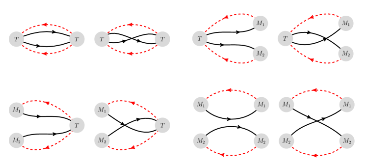
Figure 1: Nonperturbative quark-field Wick contractions for the different elements of the correlation matrix. $M_{1}$ and $M_{2}$ represent the $B$ and $B^{*}$ mesons that are separately projected to momentum zero, while $T$ represents the jointly projected operators. The black lines represent $b$-quark propagators and the red lines represent light-quark propagators.

The correlation matrix has analytical properties that follow from the symmetries of lattice QCD, in particular time reversal and charge conjugation. These symmetries imply that $(C_{jk}(t))^{\ast}=C_{kj}(t)$ and that all $C_{jk}(t)$ are real. Moreover, one can relate $C_{jk}(+t)$ and $C_{jk}(-t)$. We exploit these analytical findings to improve our lattice QCD results, by averaging related correlation functions appropriately and by setting all imaginary parts (which are pure noise) to zero.

III.2 $B$ and $B^{\ast}$ meson

Since we will compare the energy levels of the $\bar{b}\bar{b}ud$ four-quark system to the $BB^{\ast}$ threshold, we need to determine the energies of the $B$ and $B^{*}$ mesons within the same setup. We use the interpolating operators

$$O_{B}(\mathbf{p})=\sum_{\textbf{x}}e^{i\mathbf{p}\textbf{x}}\bar{b}(\textbf{x})\gamma_{5}u(\textbf{x}),$$ (10)

$$O_{B^{\ast}}(\mathbf{p})=\sum_{\textbf{x}}e^{i\mathbf{p}\textbf{x}}\bar{b}(\textbf{x})\gamma_{j}u(\textbf{x}),$$ (11)

where we also consider nonzero momenta $\mathbf{p}=2\pi\mathbf{n}/L$, $\mathbf{n}\in\mathbb{Z}^{3}$, to allow the determination of the kinetic masses (needed for the scattering analysis in Sec. VI). The quark fields are smeared with the same parameters as in Table 3. We compute the correlation functions $\langle O_{B}(\mathbf{p},t)O_{B}^{\dagger}(\mathbf{p},0)\rangle$ and $\langle O_{B^{\ast}}(\mathbf{p},t)O_{B^{\ast}}^{\dagger}(\mathbf{p},0)\rangle$. As discussed in Sec. III.1, we perform the summation over $\mathbf{x}$ at the sink only.

IV Energies and kinetic masses of the $B$ and $B^{\ast}$ mesons

We determined the energies of the $B$ and $B^{*}$ mesons from single-exponential fits of the two-point functions; the results are listed in Table 4. An example of a corresponding effective-energy plot is shown in Fig. 2. The energy of a state containing $n_{b}$ bottom quarks is shifted by $n_{b}$ times the NRQCD energy shift, which at tree-level would be equal to $-m_{b}$. This energy shift is not known with high precision, but cancels in energy differences with matching numbers of bottom quarks, including the quantities of interest in the following sections: $E_{n}-E_{B}-E_{B^{*}}$, where $E_{n}$ is the $n$-th energy level of the $\bar{b}\bar{b}ud$ system.

Ensemble	$aE_{B}(0)$	$aE_{B^{*}}(0)$	$am_{B,\,{\rm kin}}$	$am_{B^{*}\!,\,{\rm kin}}$	$E_{B^{*}}(0)-E_{B}(0)$ [MeV]	$m_{\rm kin,spinav}$ [GeV]
C00078	0.4582(45)0	0.4820(46)	3.03(14)0	3.10(13)0	41.2(5.1)	5.33(22)0
C005	0.4647(14)0	0.4944(16)	3.002(40)	2.993(42)	53.2(1.7)	5.346(73)
C01	0.4742(12)0	0.5061(16)	3.034(38)	3.030(40)	57.0(1.8)	5.409(69)
F004	0.3750(11)0	0.3975(12)	2.323(21)	2.323(25)	51.3(1.8)	5.536(57)
F006	0.37655(87)	0.3985(10)	2.320(20)	2.311(23)	52.3(1.5)	5.513(54)

Table 4: Energies of the $B$ and $B^{*}$ mesons at rest and kinetic masses computed using one quantum of momentum. Also given are the hyperfine splittings and spin-averaged kinetic masses ($m_{\rm kin,spinav}=\frac{1}{4}m_{B,\,{\rm kin}}+\frac{3}{4}m_{B^{*}\!,\,{\rm kin}}$) in physical units. All uncertainties are statistical only.

Ensemble	$c^{2}_{B}(2)$	$c^{2}_{B}(3)$	$c^{2}_{B^{*}}(2)$	$c^{2}_{B^{*}}(3)$
C00078	0.9999(13)0	0.9998(26)	1.0007(12)0	1.0014(24)
C005	1.0019(14)0	1.0036(28)	1.0014(13)0	1.0026(28)
C01	1.0015(12)0	1.0032(25)	1.0000(15)0	1.0002(30)
F004	1.00005(78)	1.0001(16)	1.00063(85)	1.0014(17)
F006	1.00032(64)	1.0007(13)	1.00030(78)	1.0005(16)

Table 5: Results for the $B$ and $B^{*}$ meson “speed of light” squared, defined in Eq. (15), for $\mathbf{p}^{2}=2(2\pi/L)^{2}$ and $\mathbf{p}^{2}=3(2\pi/L)^{2}$.

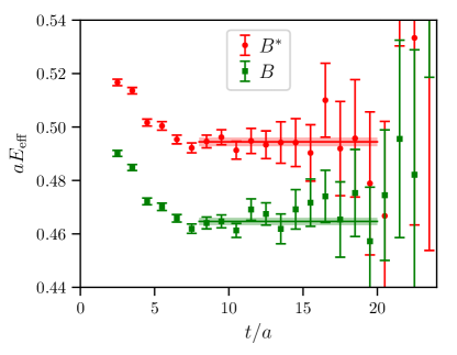
Figure 2: Effective energy plot of the $B$ and $B^{*}$ two-point functions at zero momentum computed on the C005 ensemble. The effective energy is defined as $aE_{\rm eff}(t+a/2)=\ln[C(t)/C(t+a)]$. The horizontal lines show the results of single-exponential fits to the two-point functions in the range $t/a=8...20$.

For the scattering analysis in Sec. VI (and to assess the tuning of the $b$-quark mass), we also need the momentum-dependence of the $B$ and $B^{*}$ energies. We find that within statistical uncertainties our results are consistent with the form

$$E_{B}(\mathbf{p}) = E_{B}(0)+\sqrt{m_{B,\,{\rm kin}}^{2}+\mathbf{p}^{2}}-m_{B,\,{\rm kin}}$$ (12)

$$E_{B^{*}}(\mathbf{p}) = E_{B^{*}}(0)+\sqrt{m_{B^{*}\!,\,{\rm kin}}^{2}+\mathbf{p}^{2}}-m_{B^{*}\!,\,{\rm kin}}$$ (13)

up to the highest momenta we computed ($\mathbf{p}^{2}=3(2\pi/L)^{2}$). The kinetic masses given in Table 4 were extracted using

$$m_{\rm kin}=\frac{\mathbf{p}^{2}-[E(\mathbf{p})-E(0)]^{2}}{2[E(\mathbf{p})-E(0)]}$$ (14)

with the smallest possible non-vanishing momentum, $\mathbf{p}^{2}=(2\pi/L)^{2}$. To test whether the $B$ and $B^{*}$ energies at higher momenta still satisfy the dispersion relations (12) and (13) with the same parameters, we computed the square of the “speed of light” via

$$c^{2}=\frac{[E(\mathbf{p})-E(0)+m_{\rm kin,1}]^{2}-m_{\rm kin,1}^{2}}{\mathbf{p}^{2}},$$ (15)

where $m_{\rm kin,1}$ are the kinetic masses computed with one unit of momentum. The results for $c^{2}$ are listed in Table 5 and are found to be consistent with 1 within their statistical uncertainties of 0.3% or smaller.

On the C00078 and C005 ensembles, the spin-averaged kinetic masses $m_{\rm kin,spinav}=\frac{1}{4}m_{B,\,{\rm kin}}+\frac{3}{4}m_{B^{*}\!,\,{\rm kin}}$ agree with the experimental value of 5.28272(2) GeV Tanabashi:2018oca . On the other ensembles, the lattice results are up to 5% higher, which can be attributed mainly to the following:

• The tuning of the bare $b$-quark mass was performed using bottomonium; the results here are affected by the heavier-than-physical light-quark masses and by discretization errors.

• The tuning was performed using a different determination of the lattice spacing (that of Ref. Meinel:2010pv , while here we use the lattice spacing determinations of Ref. Blum:2014tka to convert to physical units).

However, the effect of a possible $\lesssim 5\%$ mistuning of the $b$-quark mass is expected to be even smaller in the energy differences $E_{n}-E_{B}-E_{B^{*}}$ due to partial suppression by heavy-quark symmetry. The hyperfine splittings $E_{B^{*}}-E_{B}$ are of order $\Lambda/m_{b}$, and are therefore affected by the same relative error as the $b$-quark mass, which corresponds to an absolute error of $\lesssim 2.5\,\textrm{MeV}$. Our results for the hyperfine splittings are also shown in Table 4. The value from the physical-pion-mass ensemble C00078 is consistent with the experimental value of $45.3(2)\>\textrm{MeV}$ Tanabashi:2018oca . We find a trend of increasing hyperfine splitting as the light-quark mass is increased.

V The lowest energy levels of the $\bar{b}\bar{b}ud$ system

V.1 Multi-exponential matrix fitting

The spectral decomposition of the correlation matrix (9) reads

$$C_{jk}(t)=\sum_{n=0}^{\infty}\langle\Omega|O_{j}|n\rangle\langle n|O^{\dagger}_{k}|\Omega\rangle\textrm{e}^{-E_{n}t},$$ (16)

where $|\Omega\rangle$ denotes the vacuum state, $|n\rangle$ are the energy eigenstates of the $\bar{b}\bar{b}ud$ system in the $T_{1}^{g}$ irrep and for isospin $I=0$, and $E_{n}$ are the corresponding energy eigenvalues. Equation (16) assumes an infinite time extent of the lattice, which is a good approximation in our case. As discussed in Sec. III.1, all $C_{jk}(t)$ are real and, thus, so are the overlap factors

$$Z_{j}^{n}=\langle\Omega|O_{j}|n\rangle.$$ (17)

To extract the energies $E_{n}$ from our numerical results for $C_{jk}(t)$, we perform fully correlated, least-$\chi^{2}$, multi-exponential fits using a truncated version of (16),

$$C_{jk}(t)\approx\sum_{n=0}^{N-1}Z_{j}^{n}Z_{k}^{n}\textrm{e}^{-E_{n}t},$$ (18)

where we must choose the time range $t_{\textrm{min}}\leq t\leq t_{\textrm{max}}$ such that contributions from higher excited states are negligible. To enforce the ordering of the $E_{n}$ returned from the fit, for $n>0$ we actually use the logarithms of the energy differences, $l_{n}=\ln(aE_{n}-aE_{n-1})$, as our fit parameters. Furthermore, we rewrote the overlap factors for $n>0$ as $Z_{n}=B_{n}Z_{0}$ and used $B_{n}$ as the fit parameters. Note that $C_{jk}(t)$ does not need to be a square matrix. In particular, the multi-exponential matrix fit method allows us to also include correlation matrix elements $C_{jk}(t)$ with $j=4,5$ and $k=1,2,3$, i.e. the scattering operators $O_{4}$ and $O_{5}$. An example of such a $(5\times 3)$ matrix fit is shown in Fig. 3. On each ensemble, we performed fits to the full matrix as well as to various sub-matrices, for different fit ranges and different numbers of states. The results are listed in Tables 8-12 in Appendix A.

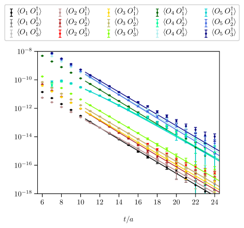
Figure 3: Example of a multi-exponential matrix fit for the C005 ensemble. This fit has $N=3$, $t_{\rm min}/a=11$, $t_{\rm max}/a=24$, and gives $\chi^{2}/{\rm d.o.f.}\approx 1.08$.

The matrix fits have a large number of degrees of freedom, and the covariance matrix, whose inverse enters in $\chi^{2}$, can become poorly determined or singular if the number of statistical samples used to estimate this matrix is not much larger than the number of degrees of freedom. This is particularly problematic when using all-mode-averaging (or, more generally, covariant-approximation-averaging, CAA), where the samples are given by Blum:2012uh ; Shintani:2014vja

$$(\text{CAA sample})_{e}=(\text{exact sample})_{e}-(\text{sloppy sample})_{e,0}+\frac{1}{N_{\text{sloppy}}}\sum_{s=0}^{N_{\text{sloppy}}-1}(\text{sloppy sample})_{e,s}.$$ (19)

Here, $e$ labels the exact samples (gauge-link configuration and source location), and the different sloppy samples, computed from quark propagators with reduced solver precision, in our case originate from applying many space-time displacements $s$ to the initial source location $e$, with $s=0$ corresponding to no displacement. As shown in Table 1, the number of exact samples, and hence CAA samples, is as low as 80 in the case of the C00078 ensemble. To obtain a meaningful $\chi^{2}$ even for large numbers of degrees of freedom, we use a “modified CAA” (MCAA) procedure, given by

$$(\text{MCAA sample})_{e,s}=(\text{exact sample})_{e}-(\text{sloppy sample})_{e,0}+(\text{sloppy sample})_{e,s}.$$ (20)

This procedure provides $N_{\text{sloppy}}$ $(=32$ in our case) times as many samples as the standard CAA procedure, without changing the overall average, and allows robust matrix fits even in the $(5\times 3)$ case. The drawback is that there are autocorrelations between the different choices of $s$, introduced by the constant (but very small) term $(\text{exact sample})_{e}-(\text{sloppy sample})_{e,0}$ and by any possible autocorrelations between the different sloppy samples on the same configuration. As a result of these autocorrelations, the uncertainties of parameters obtained from fits based on the MCAA procedure are initially slightly underestimated. We correct for these autocorrelations by rescaling all uncertainties in the fitted $E_{n}$ with a factor estimated for each ensemble using the simple $B$ meson two-point functions. The factor is given by the ratio of uncertainties of the $B$ meson energies obtained from single-exponential fits using the CAA and MCAA procedures. The factors range from 1.08 to 1.27. The uncertainties of all results shown in this paper are already corrected with these factors.

The condition numbers of the data covariance matrices range from approximately $10^{6}$ to $10^{15}$, depending on how many interpolating operators are included and on the fit range. We always computed the full inverse using LU decomposition. The minimization of $\chi^{2}$ was performed using the Levenberg-Marquardt algorithm, with initial guesses for the fit parameters obtained as described in Sec. V B of Ref. Alexandrou:2017mpi . The fit results were stable under variations of the initial guesses within reasonable ranges.

As a cross-check of the multi-exponential matrix fitting method, we also determined the spectrum using the variational approach, which involves solving the generalized eigenvalue problem (GEVP) Luscher:1990ck ; Blossier:2009kd ; Orginos:2015tha . We found that the GEVP method, where applicable, gives results consistent with the direct multi-exponential matrix fits. The comparison of the two methods is presented in Appendix B.

V.2 Dependence of the fit results on the choices of interpolating fields

Even though the actual energy levels for a chosen set of quantum numbers are independent of the interpolating operators used in the two-point functions, in practice the numerical results depend on these choices, due to limited statistical precision. In Fig. 4 we present the two lowest energy levels relative to the $BB^{\ast}$ threshold as determined on ensemble C005 using multi-exponential matrix fitting. The interpolators used are indicated by the five bars below each column. The three black bars at the bottom correspond to the local interpolators $O_{1}$, $O_{2}$, $O_{3}$, while the two red bars at the top correspond to the nonlocal interpolators $O_{4}$ and $O_{5}$. A filled bar indicates that an interpolator is included, an empty bar that it is not included. Two things are evident from Fig. 4: first, stable results for the two lowest energy levels are only obtained once the nonlocal two-meson interpolators are included in the analysis; second, once the nonlocal interpolators are included, the estimates of both the ground-state energy and the first excited energy drop significantly. Both observations clearly indicate the importance of the nonlocal interpolators for our study of the $\bar{b}\bar{b}ud$ system. Note that the first excited energy is close to the $BB^{\ast}$ threshold, while the ground state energy is significantly below threshold. This is a first indication that the ground state corresponds to a stable tetraquark, while the first excitation corresponds to a meson-meson scattering state. Similar plots for the other four ensembles are collected in Appendix A.

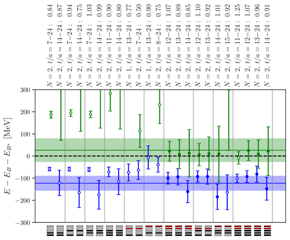
Figure 4: Results for the lowest two $\bar{b}\bar{b}ud$ energy levels relative to the $BB^{\ast}$ threshold, $\Delta E_{n}=E_{n}-E_{B}-E_{B^{*}}$, as determined on ensemble C005 from several different fits. The five bars below each column indicate the interpolators used, as explained in the main text. Above each column, we give the number of exponentials, the fit range, and the value of $\chi^{2}/\textrm{d.o.f.}$. The shaded horizontal bands correspond to our final estimates of $\Delta E_{0}$ and $\Delta E_{1}$, obtained from a bootstrap average of the subset of fits that are shown with filled symbols.

V.3 Overlap factors

For a given $j$, the overlap factors $Z_{j}^{n}$ indicate the relative importance of the energy eigenstates $|n\rangle$ when expanding the trial state $O_{j}^{\dagger}|\Omega\rangle$ in terms of energy eigenstates,

$$O_{j}^{\dagger}|\Omega\rangle=\sum_{n=0}^{\infty}|n\rangle\langle n|\mathcal{O}_{j}^{\dagger}|\Omega\rangle=\sum_{n=0}^{\infty}Z_{j}^{n}|n\rangle.$$ (21)

Therefore, the overlap factors $Z_{j}^{n}$ provide certain information about the composition and quark arrangement of the energy eigenstates $|n\rangle$. In particular, if the overlap factor $Z_{j}^{m}$ for one state $|m\rangle$ is significantly larger than all other $Z_{j}^{n}$, $n\neq m$, this might be a sign that $|m\rangle$ is quite similar to $O_{j}^{\dagger}|\Omega\rangle$.

It is convenient to consider rescaled squared overlap factors,

$$|\tilde{Z}_{j}^{n}|^{2}=\frac{|Z_{j}^{n}|^{2}}{\textrm{max}_{m}(|Z_{j}^{m}|^{2})},$$ (22)

which are normalized such that $\textrm{max}_{m}(|\tilde{Z}_{j}^{m}|^{2})=1$ for each trial state $O_{j}^{\dagger}|\Omega\rangle$. Here, the indices $n$ and $m$ can take on values from 0 to $N-1$, where $N$ is the number of states included in the fit. The results for $|\tilde{Z}_{j}^{n}|^{2}$ obtained from our fits are qualitatively similar for all ensembles, and do not strongly depend on the temporal fit range $t_{\textrm{min}}\leq t\leq t_{\textrm{max}}$.

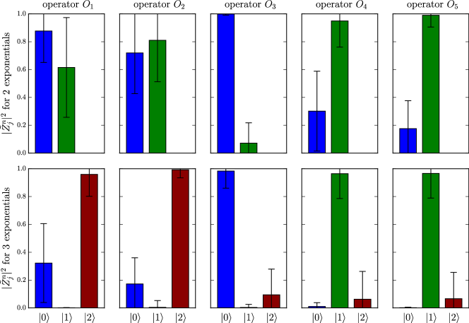
Figure 5: The normalized overlap factors $|\tilde{Z}_{j}^{n}|^{2}$ as determined on ensemble C005, indicating the relative contributions of the energy eigenstates $|n\rangle$ to the trial state $\mathcal{O}_{j}^{\dagger}|\Omega\rangle$. The upper row corresponds to a two-exponential fit with $14\leq t/a\leq 24$, while the lower row corresponds to a three-exponential fit with $12\leq t/a\leq 24$. The mean values and variances of the $|\tilde{Z}_{j}^{n}|^{2}$ were evaluated using bootstrap resampling of the fits, which explains why the mean of the largest factor can be smaller than 1.

In Fig. 5 we show the normalized overlap factors obtained on ensemble C005 using the full $5\times 3$ correlation matrix for $N=2$ and $N=3$, with fit ranges of $14\leq t/a\leq 24$ and $12\leq t/a\leq 24$, respectively. One can see that for the trial state created by the diquark-antidiquark operator $O_{3}$, the ground-state overlap is significantly larger than the overlap to the first excited state. Vice versa, for the two trial states created by the nonlocal meson-meson operators $O_{4}$ and $O_{5}$, the overlaps to the first excited state are larger than the ground-state overlaps. This supports our above interpretation concerning the composition of the lowest two energy eigenstates: the ground state $|0\rangle$ seems to be a four-quark bound state and the first excitation $|1\rangle$ a meson-meson scattering state. Finally, it is interesting to note that in the three-exponential fit, the local meson-meson operators $O_{1}$ and $O_{2}$ appear to produce a large overlap with the second excited state, while the diquark-antidiquark operator $O_{3}$ and the nonlocal operators $O_{4}$ and $O_{5}$ do not (also note that the large values of $|Z_{1}^{2}|^{2}/|Z_{1}^{0}|^{2}=4\pm 5$, $|Z_{2}^{2}|^{2}/|Z_{2}^{0}|^{2}=8\pm 9$ substantially change the normalization of the plots for $O_{1}$ and $O_{2}$ when going from $N=2$ to $N=3$). What appears in the fit as the “second excited state” (with a rather high energy and large uncertainty, as shown in Table 9) is likely an admixture of the dense spectrum of all the scattering states above threshold, which are all created with similar weights by the local operators $O_{1}$ and $O_{2}$, while the nonlocal operators $O_{4}$ and $O_{5}$ mostly create the lowest-lying scattering state.

V.4 Final results for the lowest two energy levels on each ensemble

To obtain final results for the energy differences $\Delta E_{0}$ and $\Delta E_{1}$ on each ensemble, we select a subset of fits that we deem reliable, based on the discussion in the previous two subsections and based on $\chi^{2}/{\rm d.o.f.}$. All of these fits, which are indicated with filled symbols in Fig. 4 and Figs. 9-12, include at least one of the nonlocal interpolating operators $O_{4}$ and $O_{5}$. We then repeat all selected fits for 500 bootstrap samples, where each bootstrap sample consists of randomly drawn gauge-link configurations and source locations (using the same random numbers for the different types of fits to preserve correlations). This produces 500 samples for $\Delta E_{0}$ and $\Delta E_{1}$ for each type of fit (and on each ensemble). We then average these values over the different types of fits with equal weights, bootstrap sample by bootstrap sample. Finally, we compute the mean and standard deviation (rescaled again by the MCAA autocorrelation correction factors; see the discussion in Sec. V.1) of these new 500 samples. The results for $\Delta E_{0}$ and $\Delta E_{1}$ obtained in this way are listed in Table 6 and are indicated with the horizontal lines and shaded uncertainty bands in Fig. 4 and Figs. 9-12.

Ensemble	$a\Delta E_{0}$	$a\Delta E_{1}$	$\Delta E_{0}$ [MeV]	$\Delta E_{1}$ [MeV]
C00078	$-0.075(16)$	$\phantom{+}0.001(21)$	$-129(27)$	$\phantom{+0}2(36)$
C005	$-0.069(19)$	$\phantom{+}0.015(30)$	$-123(34)$	$\phantom{+}27(53)$
C01	$-0.061(15)$	$-0.014(22)$	$-109(26)$	$-26(39)$
F004	$-0.051(11)$	$-0.011(15)$	$-122(25)$	$-25(37)$
F006	$-0.037(12)$	$\phantom{+}0.025(32)$	$-88(29)$	$\phantom{+}61(76)$

Table 6: Final results for the lowest two energy levels of the $\bar{b}\bar{b}ud$ system on each ensemble, in lattice units and in MeV. All results are given relative to the $BB^{*}$ threshold, i.e. $\Delta E_{n}=E_{n}-E_{B}-E_{B^{*}}$.

VI Scattering analysis

The energies $E_{n}$ determined in a spectroscopy computation can be related to the infinite-volume scattering amplitude using Lüscher’s method Luscher:1990ux and its generalizations Rummukainen:1995vs ; Kim:2005gf ; Christ:2005gi ; Hansen:2012tf ; Leskovec:2012gb ; Gockeler:2012yj ; Briceno:2014oea ; Briceno:2017tce ; see Ref. Briceno:2017max for a recent review. Here, we apply Lüscher’s method to the lowest two energy levels of the $\bar{b}\bar{b}ud$ system in the $T_{1}^{g}$ irrep, assuming that these energy levels can be described in terms of the elastic $S$-wave $B$-$B^{*}$ scattering amplitude (and its analytic continuation below threshold). We neglect higher partial waves and the coupling to other channels, such as $B^{*}B^{*}$. Thus, we obtain the $S$-wave $B$-$B^{*}$ scattering amplitude for the two scattering momenta $k_{0}$ and $k_{1}$ that correspond to $E_{0}$ and $E_{1}$. Having only these two points limits the choice of parametrization of the scattering amplitude to a function with two parameters, for which we use the effective-range expansion (ERE). The ERE parametrization then allows us to determine the infinite-volume bound-state energy.

VI.1 Relation between finite-volume energy levels and infinite-volume phase shifts

We define the scattering momentum $k_{n}$ corresponding to the $n$-th energy level of the $\bar{b}\bar{b}ud$ system $E_{n}$ through the equation

$$E_{n}=E_{B}+\sqrt{m_{B,\,{\rm kin}}^{2}+k_{n}^{2}}-m_{B,\,{\rm kin}}+E_{B^{*}}+\sqrt{m_{B^{*}\!,\,{\rm kin}}^{2}+k_{n}^{2}}-m_{B^{*}\!,\,{\rm kin}},$$ (23)

where $E_{B}=E_{B}(0)$ and $E_{B^{*}}=E_{B^{*}}(0)$ are the energies of the single-$B$ meson and single-$B^{*}$ meson states at zero momentum. Solving for $k_{n}^{2}$ gives

$$k_{n}^{2}=\frac{\Delta E_{n}(\Delta E_{n}+2m_{B,\,{\rm kin}})(\Delta E_{n}+2m_{B^{*}\!,\,{\rm kin}})(\Delta E_{n}+2m_{B,\,{\rm kin}}+2m_{B^{*}\!,\,{\rm kin}})}{4(\Delta E_{n}+m_{B,\,{\rm kin}}+m_{B^{*}\!,\,{\rm kin}})^{2}},$$ (24)

where

$$\Delta E_{n}=E_{n}-E_{B}-E_{B^{*}}.$$ (25)

The mapping between the finite-volume scattering momentum in the rest frame and the infinite-volume scattering amplitude expressed as the $S$-wave scattering phase shift $\delta_{0}$ is

$$\cot{\delta_{0}(k_{n})}=\frac{2Z_{00}(1;(k_{n}L/2\pi)^{2})}{\pi^{1/2}k_{n}L},$$ (26)

where $Z_{00}$ is the generalized zeta function Luscher:1990ux . The scattering amplitude is given by

$$T_{0}(k)=\frac{1}{\cot\delta_{0}(k)-i}.$$ (27)

VI.2 Effective-range expansion and determination of the bound-state pole

On each ensemble, we use the lattice QCD results for the energy differences $\Delta E_{0}$ and $\Delta E_{1}$ combined with the corresponding results for the $B$ and $B^{*}$ meson energies and kinetic masses to calculate $k_{n}^{2}$ for $n=0$ and $n=1$ using Eq. (24), and we determine the corresponding $k_{n}\cot\delta_{0}(k_{n})$ using Eq. (26). We parametrize the scattering amplitude using the effective-range expansion (ERE),

$$k\cot\delta_{0}(k)=\frac{1}{a_{0}}+\frac{1}{2}r_{0}k^{2}+\mathcal{O}(k^{4}),$$ (28)

and determine the two parameters $a_{0}$ (the $S$-wave scattering length) and $r_{0}$ (the $S$-wave effective range). Bound states correspond to poles in the scattering amplitude (27) below threshold, where $-ik>0$. Such a pole occurs for $\cot\delta_{0}(k_{\rm BS})=i$, where $k_{\rm BS}$ is the (imaginary) bound-state momentum. Combining this condition with the ERE then gives

$$-|k_{\rm BS}|=\frac{1}{a_{0}}-\frac{1}{2}r_{0}|k_{\rm BS}|^{2},$$ (29)

where terms of $\mathcal{O}(|k_{\rm BS}|^{4})$ are neglected. We solve Eq. (29) for $|k_{\rm BS}|$ and obtain the binding energy via

$$E_{\rm binding}=E_{\rm BS}-E_{B}-E_{B^{*}} =\sqrt{m_{B,\,{\rm kin}}^{2}+k_{\rm BS}^{2}}-m_{B,\,{\rm kin}}+\sqrt{m_{B^{*}\!,\,{\rm kin}}^{2}+k_{\rm BS}^{2}}-m_{B^{*}\!,\,{\rm kin}}$$ (30)

$$=\sqrt{m_{B,\,{\rm kin}}^{2}-|k_{\rm BS}|^{2}}-m_{B,\,{\rm kin}}+\sqrt{m_{B^{*}\!,\,{\rm kin}}^{2}-|k_{\rm BS}|^{2}}-m_{B^{*}\!,\,{\rm kin}}.$$ (31)

This approach was previously utilized in Refs. Beane:2010em ; Mohler:2013rwa ; Lang:2014yfa ; Moir:2016srx . Determining masses of bound states in this way is equivalent to taking the infinite-volume limit up to exponentially small finite-volume corrections proportional to $e^{-|k_{\rm BS}|L}$ (for more details, see, for example, Refs. Sasaki:2006jn ; Beane:2011iw ).

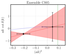
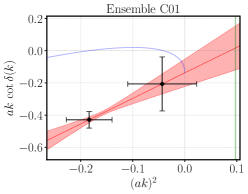
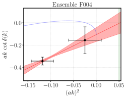
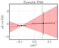
Figure 6: Plots of the effective-range-expansions. Here, $a$ denotes the lattice spacing. The straight red line going through the data points corresponds to the ERE parametrization of $ak\cot\delta(k)$. Below the $BB^{*}$ threshold (which is located at $k=0$), we also show the curves $ak\cot\delta(k)+|ak|$ [again using the ERE parametrization for $ak\cot\delta(k)$], whose lowest zero gives the binding momentum. The vertical green lines show the location of the inelastic $B^{*}B^{*}$ threshold.

VI.3 Numerical results

In Fig. 6 we show $k\cot\delta_{0}(k)=1/a_{0}+r_{0}k^{2}/2$ as a function of the scattering momentum $k$ together with the corresponding lattice data points, for the five different ensembles. One can see that $k\cot\delta_{0}(k)$ is consistent with zero within uncertainties at $k=0$, which implies an inverse scattering length also consistent with zero. The results for the inverse scattering length $1/a_{0}$, the effective range $r_{0}$, the binding momentum $|k_{\rm BS}|$, and the binding energy $E_{\textrm{binding}}$ are given in Table 7. The binding energies are essentially identical to the finite-volume energy differences $\Delta E_{0}$ collected in Table 6. This supports our interpretation of the ground state as a stable tetraquark. We also applied the consistency check proposed in Ref. Iritani:2017rlk , but our statistical uncertainties are too large to reach a definitive conclusion.

As indicated in Fig. 6, the first excited state is close to the inelastic $B^{*}B^{*}$ threshold for some of the data sets, which means that the single-channel analysis performed here is not well justified. A coupled-channel analysis is not feasible with the data we have, but is unlikely to significantly affect the results for the bound state.

Ensemble	$1/a_{0}$ [fm-1]	$r_{0}$ [fm]	$|k_{\rm BS}|$ [MeV]	$E_{\textrm{binding}}$ [MeV]
C00078	$-0.7(11.0)$	$0.4(1.3)\phantom{.}$	$824(89)\phantom{0}$	$-129(28)$
C005	$\phantom{+}0.2(7.2)\phantom{0}$	$0.51(88)$	$808(110)$	$-123(34)$
C01	$-1.24(77)\phantom{.}$	$0.35(12)$	$765(91)\phantom{0}$	$-109(26)$
F004	$-1.28(76)\phantom{.}$	$0.33(10)$	$819(85)\phantom{0}$	$-122(25)$
F006	$-0.9(10.9)$	$0.4(1.8)\phantom{.}$	$697(113)$	$-88(29)\phantom{0}$

Table 7: The inverse scattering length $1/a_{0}$, the effective range $r_{0}$, the binding momentum $|k_{\rm BS}|$, and the binding energy $E_{\textrm{binding}}$ for all ensembles.

VII Fit of the pion-mass dependence and estimates of systematic uncertainties

Given the statistical uncertainties in our results for $E_{\textrm{binding}}$ (shown in Table 7), we cannot resolve any significant dependence on the lattice spacing or pion mass. We expect lattice discretization errors to be at the level of a few MeV, as discussed further below. Since this is well below our statistical uncertainties, we choose to perform a fit of the pion-mass dependence of our results from all ensembles without including $a$-dependence. We consider a quadratic pion-mass dependence, corresponding to linear dependence on the light-quark mass,

$$E_{\textrm{binding}}(m_{\pi})=E_{\textrm{binding}}(m_{\pi,\text{phys}})+c(m_{\pi}^{2}-m_{\pi,\text{phys}}^{2}),$$ (32)

where we use $m_{\pi,\text{phys}}=135\,\textrm{MeV}$ for the physical pion mass in the isospin-symmetric limit. The fit gives

$$E_{\textrm{binding}}(m_{\pi,\text{phys}})=(-128\pm 24)\,\textrm{MeV},\quad\quad c=(1.5\pm 2.3)\times 10^{-4}\,\textrm{MeV}^{-2},$$ (33)

and has $\chi^{2}/{\rm d.o.f.}=0.27$. A plot of the fit function together with the data is shown in Fig. 7. Given that, (i), the fit has excellent quality, (ii), the resulting coefficient $c$ is consistent with zero, and (iii), the result for $E_{\textrm{binding}}(m_{\pi,\text{phys}})$ is nearly identical with the result from the C00078 ensemble with $m_{\pi}=139(1)$ MeV, we conclude that any remaining systematic uncertainties associated with the extrapolation to $m_{\pi,\text{phys}}$ are negligible.

The lattice discretization errors associated with our light-quark and gluon actions and are expected to be at the 1% level for the fine lattices, and at the 2% level for the coarse lattices Blum:2014tka ; multiplying by the QCD scale of $\Lambda\sim 300\,\textrm{MeV}$ yields $3\,\textrm{MeV}$ to $6\,\textrm{MeV}$. The NRQCD action introduces additional systematic uncertainties. For our choice of lattice discretization and matching coefficients, the most significant systematic errors in the energy of a heavy-light hadron are expected to be the following:

• Four-quark operators, which arise at order $\alpha_{s}^{2}$ in the matching to full QCD, are not included in the action. The analysis of Ref. Blok:1996iz suggests that their effects could be as large as $3\,\textrm{MeV}$.

• The matching coefficient $c_{4}$ of the operator $-\frac{g}{2m_{b}}\>{\boldsymbol{\sigma}}\cdot\mathbf{B}$ was computed to one loop. Missing higher-order corrections to this coefficient introduce systematic errors of order

  $$\alpha_{s}^{2}\Lambda^{2}/m_{b}\approx 2\,{\rm MeV}.$$ (34)

• The matching coefficients of the operators of order $(\Lambda/m_{b})^{2}$ were computed at tree-level only. The missing radiative corrections to these coefficients introduce systematic errors of order

  $$\alpha_{s}\Lambda^{3}/m_{b}^{2}\approx 0.4\,{\rm MeV}.$$ (35)

These estimates are appropriate for $E_{B}$ and $E_{B^{*}}$, which contribute to our calculation of the binding energy via $E_{\rm binding}=E_{\rm BS}-E_{B}-E_{B^{*}}$. For the tetraquark energy $E_{\rm BS}$, the power counting is more complicated due to the presence of two bottom quarks. Conservative estimates of the systematic errors can be obtained by replacing the scale $\Lambda$ in the heavy-light power counting by the binding momentum $|k_{\rm BS}|\sim 800$ MeV, which suggests systematic errors of order 10 MeV. It is likely that there is a partial cancellation of the systematic errors in $E_{\rm binding}=E_{\rm BS}-E_{B}-E_{B^{*}}$. Therefore, we estimate the overall discretization and heavy-quark systematic errors to be not larger than $10\,\textrm{MeV}$ (in future work, the estimates of the heavy-quark errors could be made more precise by numerically investigating the dependence of $E_{\textrm{binding}}$ on the lattice NRQCD matching coefficients). Our final results for the tetraquark binding energy and mass are therefore

$$E_{\textrm{binding}}(m_{\pi,\text{phys}})=(-128\pm 24\pm 10)\,\textrm{MeV},\quad\quad m_{\textrm{tetraquark}}(m_{\pi,\text{phys}})=(10476\pm 24\pm 10)\,\textrm{MeV},$$ (36)

where $m_{\textrm{tetraquark}}$ is obtained by adding the experimental values of the $B$ and $B^{*}$ masses Tanabashi:2018oca to $E_{\textrm{binding}}$.

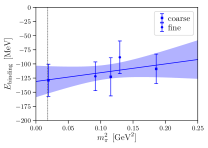
Figure 7: Fit of the pion-mass dependence of $E_{\textrm{binding}}$. The vertical dashed line indicates the physical pion mass.

VIII Conclusions

In this work we computed the low-lying spectrum in the bottomness-$2$ and $I(J^{P})=0(1^{+})$ sector. Using both local and nonlocal interpolating operators, we determined the two lowest energy levels for five different ensembles of lattice gauge-link configurations, including one with approximately physical light-quark masses. We carried out a Lüscher analysis for the first time in this sector and used the effective-range expansion to find the infinite-volume binding energies (but we found these to be nearly identical to the finite-volume binding energies). Our calculation confirms the existence of a $\bar{b}\bar{b}ud$ bound state that is stable under the strong and electromagnetic interactions.

In Fig. 8 we compare our result (36) for the binding energy with several previous determinations. These include direct lattice QCD calculations that also treated the heavy $\bar{b}$ quarks with NRQCD Francis:2016hui ; Junnarkar:2018twb , calculations in the Born-Oppenheimer approximation using static $\bar{b}\bar{b}$ potentials (in the presence of $u$ and $d$ valence quarks) computed on the lattice Bicudo:2012qt ; Brown:2012tm ; Bicudo:2016ooe , as well as the studies of Refs. Carlson:1987hh ; SilvestreBrac:1993ss ; Brink:1998as ; Vijande:2003ki ; Janc:2004qn ; Vijande:2006jf ; Navarra:2007yw ; Ebert:2007rn ; Zhang:2007mu ; Lee:2009rt ; Karliner:2017qjm ; Eichten:2017ffp ; Wang:2017uld ; Park:2018wjk ; Wang:2018atz ; Liu:2019stu , which are based on quark models, effective field theories, or QCD sum rules.

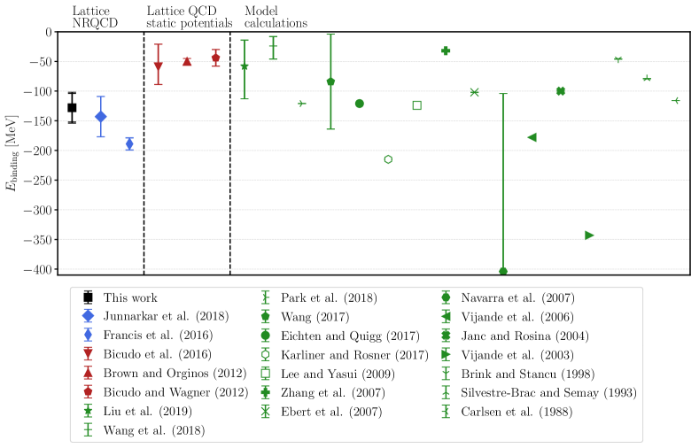
Figure 8: Comparison of results for the binding energy of the $\bar{b}\bar{b}ud$ tetraquark with $I(J^{P})=0(1^{+})$ (black: this work, using lattice NRQCD; blue: previous work using lattice NRQCD Francis:2016hui ; Junnarkar:2018twb ; red: lattice QCD computations of static $\bar{b}\bar{b}$ potentials and solving the Schrödinger equation Bicudo:2012qt ; Brown:2012tm ; Bicudo:2016ooe ; green: quark models, effective field theories, and QCD sum rules Carlson:1987hh ; SilvestreBrac:1993ss ; Brink:1998as ; Vijande:2003ki ; Janc:2004qn ; Vijande:2006jf ; Navarra:2007yw ; Ebert:2007rn ; Zhang:2007mu ; Lee:2009rt ; Karliner:2017qjm ; Eichten:2017ffp ; Wang:2017uld ; Park:2018wjk ; Wang:2018atz ; Liu:2019stu .

The calculations using static $\bar{b}\bar{b}$ potentials from lattice QCD Bicudo:2012qt ; Brown:2012tm ; Bicudo:2016ooe consistently give a binding energy that is about a factor of 2 smaller than our result (36), but this disagreement might be due the approximations used there, in particular the neglect of $1/m_{b}$ corrections to the potentials.

The two previous direct lattice QCD calculations Francis:2016hui ; Junnarkar:2018twb employed only local four-quark interpolating operators. According to our observations, the lack of nonlocal operators can affect the reliability of the extracted ground-state energy, as the local operators are not well suited to isolate the lowest $BB^{*}$ threshold state. While the result of Ref. Junnarkar:2018twb agrees with ours, Ref. Francis:2016hui gives a significantly larger binding energy. Apart from the lack of nonlocal interpolating operators, another possible source of this discrepancy might be the use of ratios of correlation functions as input to the generalized eigenvalue problem in Ref. Francis:2016hui . It is interesting to observe that the effective energies shown in Refs. Francis:2016hui ; Junnarkar:2018twb approach the ground state from below, corresponding to a decrease in the magnitude of the extracted binding energy as the time separation is increased. Both of these studies used wall sources for the quark fields, while we use Gaussian-smeared sources. These two types of sources can behave quite differently with regard to excited-state contamination Yamazaki:2017jfh . Furthermore, the excited-state spectrum of $B$-$B^{*}$ and $B^{*}$-$B^{*}$ scattering states above threshold is very dense, because the changes in the kinetic energy when increasing the back-to-back momenta are suppressed by the heavy-meson masses. For example, on a lattice with $L=6\>{\rm fm}$, the energy difference between the threshold and next scattering state is only around $8\,\textrm{MeV}$. In the context of two-nucleon systems, it has been argued that the dense spectrum can lead to “fake plateaus” at short time separations in the effective energies from ratios of correlation functions Iritani:2016jie ; see Ref. Davoudi:2017ddj for a critical discussion of this issue.

Even though our work has improved upon previous studies of the $\bar{b}\bar{b}ud$ system by including nonlocal meson-meson scattering operators at the sink, our fits still require rather large time separations, leading to large statistical uncertainties. As demonstrated for the case of the $H$ dibaryon in Ref. Francis:2018qch , the results can be vastly improved by including nonlocal operators at both source and sink, and by including additional back-to-back momenta to map out a larger region of the spectrum. This requires more advanced techniques Peardon:2009gh ; Abdel-Rehim:2017dok for constructing the correlation functions.

Appendix A The two lowest energy levels for all ensembles

In Figs. 9-12 we show the two lowest energy levels for the ensembles C00078, C01, F004, and F006. The style is identical to Fig. 4, where the same energy levels are shown for ensemble C005, and which is discussed in detail in Sec. V.3. The numerical results of the fits for all ensembles are given in Tables 8-12.

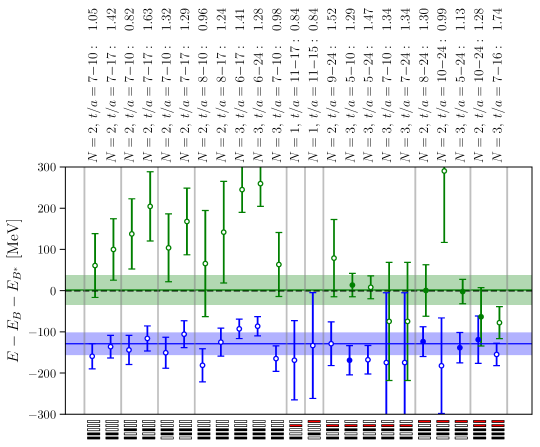
Figure 9: Like Fig. 4, but for the C00078 ensemble.

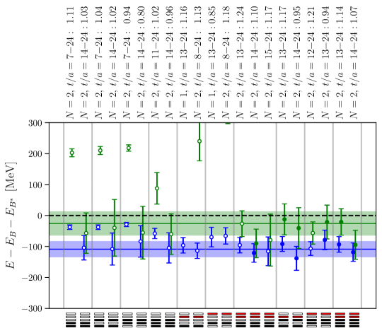
Figure 10: Like Fig. 4, but for the C01 ensemble.

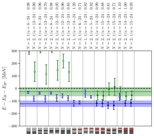
Figure 11: Like Fig. 4, but for the F004 ensemble.

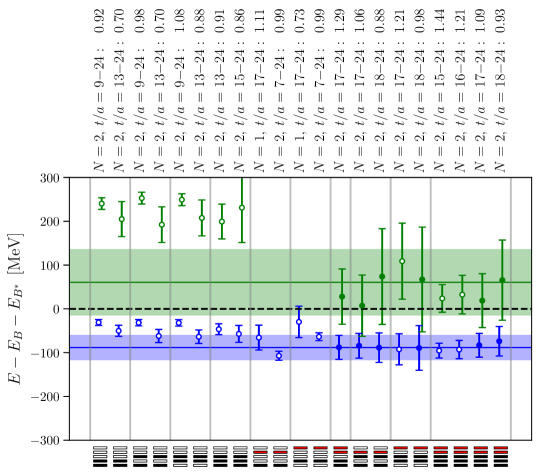
Figure 12: Like Fig. 4, but for the F006 ensemble.

Matrix	$N$	Fit range	$\chi^{2}/{\rm d.o.f.}$	$E_{n}-E_{B}-E_{B^{*}}$ [MeV]
$(O_{1},O_{2})\times(O_{1},O_{2})$	2	7…10	1.05	$-159(31)$,	$+61(77)$
$(O_{1},O_{2})\times(O_{1},O_{2})$	2	7…17	1.42	$-136(27)$,	$+100(75)$
$(O_{1},O_{3})\times(O_{1},O_{3})$	2	7…10	0.82	$-144(35)$,	$+137(85)$
$(O_{1},O_{3})\times(O_{1},O_{3})$	2	7…17	1.63	$-116(30)$,	$+204(84)$
$(O_{2},O_{3})\times(O_{2},O_{3})$	2	7…10	1.32	$-151(38)$,	$+104(82)$
$(O_{2},O_{3})\times(O_{2},O_{3})$	2	7…17	1.29	$-106(33)$,	$+168(81)$
$(O_{1},O_{2},O_{3})\times(O_{1},O_{2},O_{3})$	2	8…10	0.96	$-181(40)$,	$+66(129)$
$(O_{1},O_{2},O_{3})\times(O_{1},O_{2},O_{3})$	2	8…17	1.24	$-125(34)$,	$+142(123)$
$(O_{1},O_{2},O_{3})\times(O_{1},O_{2},O_{3})$	3	6…17	1.41	$-93(24)$,	$+245(55)$,	$+612(328)$
$(O_{1},O_{2},O_{3})\times(O_{1},O_{2},O_{3})$	3	6…24	1.28	$-86(23)$,	$+260(55)$,	$+651(337)$
$(O_{1},O_{2},O_{3})\times(O_{1},O_{2},O_{3})$	3	7…10	0.98	$-165(31)$,	$+63(77)$,	$+6283(3782)$
$(O_{1},O_{4})\times(O_{1})$	1	11…17	0.84	$-169(96)$
$(O_{2},O_{5})\times(O_{2})$	1	11…15	0.84	$-133(128)$
$(O_{1},O_{2},O_{4},O_{5})\times(O_{1},O_{2})$	2	11…13	0.90	$-181(110)$,	$-104(199)$
$(O_{1},O_{3},O_{4})\times(O_{1},O_{3})$	2	9…15	1.81	$-125(51)$,	$+86(98)$
$(O_{1},O_{3},O_{4})\times(O_{1},O_{3})$	2	9…24	1.52	$-129(53)$,	$+79(94)$
$(O_{1},O_{3},O_{4})\times(O_{1},O_{3})$	2	10…16	1.72	$-217(85)$,	$+327(187)$
$(O_{1},O_{3},O_{4})\times(O_{1},O_{3})$	3	5…10	1.29	$-169(35)$,	$+13(28)$,	$+516(100)$
$(O_{1},O_{3},O_{4})\times(O_{1},O_{3})$	3	7…10	1.34	$-175(159)$,	$-75(143)$,	$+253(538)$
$(O_{1},O_{3},O_{4})\times(O_{1},O_{3})$	3	5…16	1.55	$-169(35)$,	$+7(28)$,	$+479(89)$
$(O_{1},O_{3},O_{4})\times(O_{1},O_{3})$	3	5…24	1.47	$-168(35)$,	$+8(27)$,	$+483(88)$
$(O_{1},O_{3},O_{4})\times(O_{1},O_{3})$	3	7…16	1.55	$-250(120)$,	$-76(58)$,	$+312(207)$
$(O_{1},O_{3},O_{4})\times(O_{1},O_{3})$	3	7…24	1.46	$-237(97)$,	$-70(52)$,	$+372(233)$
$(O_{2},O_{3},O_{5})\times(O_{2},O_{3})$	2	8…24	1.30	$-124(36)$,	$+0(62)$
$(O_{2},O_{3},O_{5})\times(O_{2},O_{3})$	2	10…24	1.30	$-182(116)$,	$+290(173)$
$(O_{2},O_{3},O_{5})\times(O_{2},O_{3})$	3	5…10	1.52	$-146(36)$,	$+5(31)$,	$+510(105)$
$(O_{2},O_{3},O_{5})\times(O_{2},O_{3})$	3	7…10	1.99	$-163(55)$,	$-19(111)$,	$+520(708)$
$(O_{2},O_{3},O_{5})\times(O_{2},O_{3})$	3	5…16	1.40	$-134(36)$,	$+2(31)$,	$+452(95)$
$(O_{2},O_{3},O_{5})\times(O_{2},O_{3})$	3	5…24	1.13	$-138(37)$,	$-2(30)$,	$+450(92)$
$(O_{1},O_{2},O_{3},O_{4},O_{5})\times(O_{1},O_{2},O_{3})$	2	10…16	1.34	$-102(60)$,	$-54(70)$
$(O_{1},O_{2},O_{3},O_{4},O_{5})\times(O_{1},O_{2},O_{3})$	2	10…24	1.28	$-119(57)$,	$-63(71)$
$(O_{1},O_{2},O_{3},O_{4},O_{5})\times(O_{1},O_{2},O_{3})$	3	6…16	2.61	$-122(28)$,	$-21(31)$,	$+406(254)$
$(O_{1},O_{2},O_{3},O_{4},O_{5})\times(O_{1},O_{2},O_{3})$	3	6…24	2.11	$-143(54)$,	$-34(30)$,	$+359(225)$
$(O_{1},O_{2},O_{3},O_{4},O_{5})\times(O_{1},O_{2},O_{3})$	3	7…16	1.74	$-155(27)$,	$-78(39)$,	$+1736(1580)$

Table 8: Multi-exponential matrix fit results from the C00078 ensemble.

Matrix	$N$	Fit range	$\chi^{2}/{\rm d.o.f.}$	$E_{n}-E_{B}-E_{B^{*}}$ [MeV]
$(O_{1},O_{2})\times(O_{1},O_{2})$	2	7…22	0.84	$-58.7(8.2)$,	$+187(15)$
$(O_{1},O_{2})\times(O_{1},O_{2})$	2	14…24	0.87	$-121(57)$,	$+535(464)$
$(O_{1},O_{3})\times(O_{1},O_{3})$	2	7…22	0.94	$-59.1(8.8)$,	$+194(15)$
$(O_{1},O_{3})\times(O_{1},O_{3})$	2	14…24	0.75	$-165(70)$,	$+571(459)$
$(O_{2},O_{3})\times(O_{2},O_{3})$	2	7…22	1.03	$-60.6(9.1)$,	$+189(15)$
$(O_{2},O_{3})\times(O_{2},O_{3})$	2	14…24	0.99	$-175(65)$,	$+602(475)$
$(O_{1},O_{2},O_{3})\times(O_{1},O_{2},O_{3})$	2	11…24	0.90	$-72(22)$,	$+282(79)$
$(O_{1},O_{2},O_{3})\times(O_{1},O_{2},O_{3})$	2	14…24	0.80	$-116(58)$,	$+628(505)$
$(O_{1},O_{2},O_{3})\times(O_{1},O_{2},O_{3})$	3	6…24	0.88	$-50.6(7.3)$,	$+199(11)$,	$+696(74)$
$(O_{1},O_{2},O_{3})\times(O_{1},O_{2},O_{3})$	3	8…24	0.90	$-57(11)$,	$+180(20)$,	$+362(264)$
$(O_{1},O_{2},O_{3})\times(O_{1},O_{2},O_{3})$	3	14…24	0.78	$-174(93)$,	$+550(466)$,	$+1220(1642)$
$(O_{1},O_{4})\times(O_{1})$	1	13…24	0.77	$-74(39)$
$(O_{1},O_{4})\times(O_{1})$	2	7…24	0.50	$-63(43)$,	$+113(74)$
$(O_{2},O_{5})\times(O_{2})$	1	13…24	0.90	$-6(52)$
$(O_{2},O_{5})\times(O_{2})$	2	7…24	0.75	$-39(34)$,	$+232(84)$
$(O_{1},O_{2},O_{4},O_{5})\times(O_{1},O_{2})$	2	12…24	1.07	$-100(26)$,	$+22(45)$
$(O_{1},O_{2},O_{4},O_{5})\times(O_{1},O_{2})$	2	13…24	0.89	$-94(35)$,	$-8(66)$
$(O_{1},O_{2},O_{4},O_{5})\times(O_{1},O_{2})$	2	14…24	0.85	$-161(49)$,	$+13(110)$
$(O_{1},O_{3},O_{4})\times(O_{1},O_{3})$	2	12…24	1.10	$-92(25)$,	$+6(50)$
$(O_{1},O_{3},O_{4})\times(O_{1},O_{3})$	2	13…24	0.92	$-93(35)$,	$+11(75)$
$(O_{1},O_{3},O_{4})\times(O_{1},O_{3})$	3	7…24	0.85	$-59.2(8.9)$,	$+9(31)$,	$+193(16)$
$(O_{1},O_{3},O_{4})\times(O_{1},O_{3})$	3	11…24	0.79	$-106(28)$,	$-38(161)$,	$+246(119)$
$(O_{2},O_{3},O_{5})\times(O_{2},O_{3})$	2	14…24	1.01	$-184(57)$,	$+9(126)$
$(O_{2},O_{3},O_{5})\times(O_{2},O_{3})$	2	15…24	0.92	$-164(78)$,	$+302(276)$
$(O_{2},O_{3},O_{5})\times(O_{2},O_{3})$	3	6…24	1.00	$-49.9(7.8)$,	$+88(28)$,	$+204(21)$
$(O_{2},O_{3},O_{5})\times(O_{2},O_{3})$	3	8…24	0.98	$-60(11)$,	$-15(50)$,	$+178(20)$
$(O_{2},O_{3},O_{5})\times(O_{2},O_{3})$	3	10…24	1.07	$-65(29)$,	$-23(141)$,	$+219(47)$
$(O_{1},O_{2},O_{3},O_{4},O_{5})\times(O_{1},O_{2},O_{3})$	2	11…24	1.25	$-100(19)$,	$-8(28)$
$(O_{1},O_{2},O_{3},O_{4},O_{5})\times(O_{1},O_{2},O_{3})$	2	12…24	1.07	$-93(26)$,	$+25(45)$
$(O_{1},O_{2},O_{3},O_{4},O_{5})\times(O_{1},O_{2},O_{3})$	2	13…24	0.96	$-82(36)$,	$+9(64)$
$(O_{1},O_{2},O_{3},O_{4},O_{5})\times(O_{1},O_{2},O_{3})$	2	14…24	0.91	$-148(51)$,	$+22(110)$
$(O_{1},O_{2},O_{3},O_{4},O_{5})\times(O_{1},O_{2},O_{3})$	3	10…24	1.47	$-89(15)$,	$+40(122)$,	$+215(67)$
$(O_{1},O_{2},O_{3},O_{4},O_{5})\times(O_{1},O_{2},O_{3})$	3	11…24	1.08	$-97(20)$,	$+136(199)$,	$+288(160)$
$(O_{1},O_{2},O_{3},O_{4},O_{5})\times(O_{1},O_{2},O_{3})$	3	12…24	1.03	$-90(27)$,	$-14(231)$,	$+360(199)$

Table 9: Multi-exponential matrix fit results from the C005 ensemble.

Matrix	$N$	Fit range	$\chi^{2}/{\rm d.o.f.}$	$E_{n}-E_{B}-E_{B^{*}}$ [MeV]
$(O_{1},O_{2})\times(O_{1},O_{2})$	2	7…24	1.11	$-37.6(7.2)$,	$+203(13)$
$(O_{1},O_{2})\times(O_{1},O_{2})$	2	14…24	1.03	$-104(47)$,	$-57(97)$
$(O_{1},O_{3})\times(O_{1},O_{3})$	2	7…24	1.04	$-37.7(7.5)$,	$+210(13)$
$(O_{1},O_{3})\times(O_{1},O_{3})$	2	14…24	1.02	$-108(52)$,	$-40(91)$
$(O_{2},O_{3})\times(O_{2},O_{3})$	2	6…24	0.94	$-29.0(6.8)$,	$+218(10)$
$(O_{2},O_{3})\times(O_{2},O_{3})$	2	14…24	0.80	$-84(51)$,	$-55(85)$
$(O_{1},O_{2},O_{3})\times(O_{1},O_{2},O_{3})$	2	11…24	1.02	$-58(17)$,	$+88(51)$
$(O_{1},O_{2},O_{3})\times(O_{1},O_{2},O_{3})$	2	14…24	0.96	$-104(49)$,	$-60(66)$
$(O_{1},O_{2},O_{3})\times(O_{1},O_{2},O_{3})$	3	6…24	0.99	$-31.1(6.5)$,	$+211(10)$,	$+825(69)$
$(O_{1},O_{2},O_{3})\times(O_{1},O_{2},O_{3})$	3	8…24	1.04	$-36.1(8.5)$,	$+208(18)$,	$+1281(434)$
$(O_{1},O_{2},O_{3})\times(O_{1},O_{2},O_{3})$	3	10…24	1.07	$-50(13)$,	$+156(36)$,	$+2821(3773)$
$(O_{1},O_{4})\times(O_{1})$	1	13…24	1.16	$-96(25)$
$(O_{1},O_{4})\times(O_{1})$	2	8…24	1.13	$-114(25)$,	$+240(63)$
$(O_{2},O_{5})\times(O_{2})$	1	13…24	0.85	$-70(31)$
$(O_{2},O_{5})\times(O_{2})$	2	8…24	1.18	$-66(26)$,	$+394(98)$
$(O_{1},O_{2},O_{4},O_{5})\times(O_{1},O_{2})$	2	13…24	1.24	$-96(25)$,	$-26(41)$
$(O_{1},O_{2},O_{4},O_{5})\times(O_{1},O_{2})$	2	14…24	1.10	$-121(30)$,	$-90(46)$
$(O_{1},O_{2},O_{4},O_{5})\times(O_{1},O_{2})$	2	15…24	1.17	$-116(46)$,	$-79(84)$
$(O_{1},O_{3},O_{4})\times(O_{1},O_{3})$	2	13…24	1.17	$-92(24)$,	$-12(50)$
$(O_{1},O_{3},O_{4})\times(O_{1},O_{3})$	2	14…24	0.95	$-138(39)$,	$-41(66)$
$(O_{1},O_{3},O_{4})\times(O_{1},O_{3})$	3	7…24	1.19	$-36.2(6.9)$,	$+30(25)$,	$+210(11)$
$(O_{2},O_{3},O_{5})\times(O_{2},O_{3})$	2	12…24	1.21	$-107(22)$,	$-56(36)$
$(O_{2},O_{3},O_{5})\times(O_{2},O_{3})$	2	13…24	0.94	$-79(32)$,	$-21(55)$
$(O_{2},O_{3},O_{5})\times(O_{2},O_{3})$	3	6…24	1.11	$-30.0(7.5)$,	$+87(26)$,	$+244(38)$
$(O_{2},O_{3},O_{5})\times(O_{2},O_{3})$	3	8…24	1.10	$-44(12)$,	$+59(32)$,	$+322(74)$
$(O_{2},O_{3},O_{5})\times(O_{2},O_{3})$	3	10…24	1.01	$-123(64)$,	$-26(27)$,	$+241(116)$
$(O_{1},O_{2},O_{3},O_{4},O_{5})\times(O_{1},O_{2},O_{3})$	2	13…24	1.14	$-93(25)$,	$-21(43)$
$(O_{1},O_{2},O_{3},O_{4},O_{5})\times(O_{1},O_{2},O_{3})$	2	14…24	1.07	$-118(30)$,	$-95(47)$

Table 10: Multi-exponential matrix fit results from the C01 ensemble.

Matrix	$N$	Fit range	$\chi^{2}/{\rm d.o.f.}$	$E_{n}-E_{B}-E_{B^{*}}$ [MeV]
$(O_{1},O_{2})\times(O_{1},O_{2})$	2	8…24	0.98	$-31.4(8.6)$,	$+288(17)$
$(O_{1},O_{2})\times(O_{1},O_{2})$	2	13…24	0.90	$-81(21)$,	$+133(79)$
$(O_{1},O_{3})\times(O_{1},O_{3})$	2	8…24	0.96	$-37.0(9.3)$,	$+300(17)$
$(O_{1},O_{3})\times(O_{1},O_{3})$	2	13…24	0.70	$-83(25)$,	$+113(79)$
$(O_{2},O_{3})\times(O_{2},O_{3})$	2	8…24	0.98	$-36.2(9.5)$,	$+302(17)$
$(O_{2},O_{3})\times(O_{2},O_{3})$	2	13…24	0.95	$-76(28)$,	$+145(80)$
$(O_{1},O_{2},O_{3})\times(O_{1},O_{2},O_{3})$	2	12…24	0.90	$-59(17)$,	$+218(56)$
$(O_{1},O_{2},O_{3})\times(O_{1},O_{2},O_{3})$	2	13…24	0.85	$-78(21)$,	$+132(78)$
$(O_{1},O_{4})\times(O_{1})$	1	14…24	1.20	$-118(24)$
$(O_{1},O_{4})\times(O_{1})$	2	6…24	0.71	$-111(14)$,	$+370(24)$
$(O_{2},O_{5})\times(O_{2})$	1	14…24	0.82	$-42(29)$
$(O_{2},O_{5})\times(O_{2})$	2	5…24	0.82	$-67(11)$,	$+495(20)$
$(O_{1},O_{2},O_{4},O_{5})\times(O_{1},O_{2})$	2	14…22	0.99	$-120(22)$,	$-55(34)$
$(O_{1},O_{2},O_{4},O_{5})\times(O_{1},O_{2})$	2	15…22	0.88	$-119(29)$,	$-58(37)$
$(O_{1},O_{3},O_{4})\times(O_{1},O_{3})$	2	14…24	0.81	$-135(26)$,	$-5(49)$
$(O_{1},O_{3},O_{4})\times(O_{1},O_{3})$	2	15…24	0.71	$-135(34)$,	$+12(70)$
$(O_{2},O_{3},O_{5})\times(O_{2},O_{3})$	2	14…24	1.10	$-68(29)$,	$-37(51)$
$(O_{1},O_{2},O_{3},O_{4},O_{5})\times(O_{1},O_{2},O_{3})$	2	14…24	1.00	$-119(21)$,	$-61(32)$
$(O_{1},O_{2},O_{3},O_{4},O_{5})\times(O_{1},O_{2},O_{3})$	2	15…24	0.93	$-115(28)$,	$-55(34)$

Table 11: Multi-exponential matrix fit results from the F004 ensemble.

Matrix	$N$	Fit range	$\chi^{2}/{\rm d.o.f.}$	$E_{n}-E_{B}-E_{B^{*}}$ [MeV]
$(O_{1},O_{2})\times(O_{1},O_{2})$	2	9…24	0.92	$-31.0(6.8)$,	$+240(13)$
$(O_{1},O_{2})\times(O_{1},O_{2})$	2	13…24	0.90	$-50(13)$,	$+205(40)$
$(O_{1},O_{3})\times(O_{1},O_{3})$	2	9…24	0.96	$-31.6(7.2)$,	$+253(13)$
$(O_{1},O_{3})\times(O_{1},O_{3})$	2	13…24	0.70	$-62(15)$,	$+192(41)$
$(O_{2},O_{3})\times(O_{2},O_{3})$	2	9…22	1.08	$-32.0(7.5)$,	$+249(14)$
$(O_{2},O_{3})\times(O_{2},O_{3})$	2	13…24	0.88	$-64(15)$,	$+208(41)$
$(O_{1},O_{2},O_{3})\times(O_{1},O_{2},O_{3})$	2	13…24	0.91	$-47(12)$,	$+199(40)$
$(O_{1},O_{2},O_{3})\times(O_{1},O_{2},O_{3})$	2	15…24	0.86	$-57(19)$,	$+231(80)$
$(O_{1},O_{4})\times(O_{1})$	1	17…24	1.11	$-66(28)$
$(O_{1},O_{4})\times(O_{1})$	2	7…24	0.99	$-107(10)$,	$+350(21)$
$(O_{2},O_{5})\times(O_{2})$	1	17…24	0.73	$-30(36)$
$(O_{2},O_{5})\times(O_{2})$	2	6…24	0.99	$-63.6(8.9)$,	$+479(18)$
$(O_{1},O_{2},O_{4},O_{5})\times(O_{1},O_{2})$	2	17…24	1.29	$-88(27)$,	$+28(63)$
$(O_{1},O_{3},O_{4})\times(O_{1},O_{3})$	2	17…24	1.06	$-84(28)$,	$+7(70)$
$(O_{1},O_{3},O_{4})\times(O_{1},O_{3})$	2	18…24	0.88	$-89(34)$,	$+74(109)$
$(O_{2},O_{3},O_{5})\times(O_{2},O_{3})$	2	17…24	1.21	$-92(35)$,	$+109(87)$
$(O_{2},O_{3},O_{5})\times(O_{2},O_{3})$	2	18…24	0.98	$-89(51)$,	$+67(120)$
$(O_{1},O_{2},O_{3},O_{4},O_{5})\times(O_{1},O_{2},O_{3})$	2	15…24	1.44	$-95(17)$,	$+24(31)$
$(O_{1},O_{2},O_{3},O_{4},O_{5})\times(O_{1},O_{2},O_{3})$	2	16…24	1.21	$-93(21)$,	$+32(44)$
$(O_{1},O_{2},O_{3},O_{4},O_{5})\times(O_{1},O_{2},O_{3})$	2	17…24	1.09	$-83(27)$,	$+19(61)$
$(O_{1},O_{2},O_{3},O_{4},O_{5})\times(O_{1},O_{2},O_{3})$	2	18…24	0.93	$-74(34)$,	$+66(92)$

Table 12: Multi-exponential matrix fit results from the F006 ensemble.

Appendix B Comparison of multi-exponential matrix fitting and solving the GEVP

In this section we compare the multi-exponential matrix fitting method, used in the main part of this work, to the variational method Luscher:1990ck ; Blossier:2009kd ; Orginos:2015tha . The latter is based on the generalized eigenvalue problem

$$C_{jk}(t)v_{k}^{n}(t,t_{0})=\lambda^{n}(t,t_{0})C_{jk}(t_{0})v_{k}^{n}(t,t_{0}),$$ (37)

where $C_{jk}(t)$ must be a hermitian square matrix. As discussed in Sec. III.1, our use of point-to-all propagators did not allow us to compute the correlation matrix elements $C_{jk}(t)$ with $j,k\in\{4,5\}$, which means that we can only include the operators $O_{1}$ to $O_{3}$ in the GEVP analysis (in contrast, the multi-exponential matrix fitting method does not require a square matrix and allows us to include $O_{4}$ and $O_{5}$ at the sink).

For large time, the eigenvalues $\lambda^{n}(t,t_{0})$ are expected to satisfy

$$\lambda^{n}(t,t_{0})\propto\textrm{e}^{-E_{n}t},$$ (38)

where $E_{n}$ is the energy of the $n$th state. We define the effective energy $E_{\textrm{eff},n}(t)$ as

$$E_{\textrm{eff},n}(t)=\frac{1}{a}\ln\left(\frac{\lambda^{n}(t,t_{0})}{\lambda^{n}(t+a,t_{0})}\right),$$ (39)

which for large $t$ should plateau at $E_{n}$. An example for $E_{\textrm{eff},n}(t)$ is shown in Fig. 13. We determined $E_{n}$ from constant fits to $E_{\textrm{eff},n}(t)$ in a suitable range $t_{\textrm{min}}\leq t\leq t_{\textrm{max}}$ such that $\chi^{2}/\textrm{d.o.f.}\lesssim 1$. Alternatively, one can fit exponential functions $A\textrm{e}^{-E_{n}t}$ to the eigenvalues $\lambda^{n}(t,t_{0})$. We performed such fits as cross-checks and found consistent energies and statistical uncertainties.

Figure 13: Effective energies $aE_{\textrm{eff},n}$ for $n=0,1$ obtained for the C005 ensemble by solving the GEVP for the $3\times 3$ correlation matrix $C_{jk}(t)$ containing operators $O_{1}$ to $O_{3}$. The horizontal lines show the results of constant fits in the regions $t/a=8\ldots 17$ ($n=0$) and $t/a=8\ldots 14$ ($n=1$).

We compared the multi-exponential matrix-fit method and the GEVP method by determining the lowest two energy levels with both methods in the following way:

• We used the same symmetric correlation matrices: $2\times 2$ correlation matrices with operators $(O_{1},O_{2})$, $(O_{1},O_{3})$ and $(O_{2},O_{3})$ as well as the $3\times 3$ correlation matrix with operators $(O_{1},O_{2},O_{3})$.

• We used the same values for $t_{\textrm{min}}$ (larger $t_{\textrm{min}}$ leads to a stronger suppression of excited states; we performed a comparison for several values for $t_{\textrm{min}}$).

• We used similar values for $t_{\textrm{max}}$ (the results only weakly depend on $t_{\textrm{max}}$; we chose $t_{\textrm{max}}$ as the largest temporal separation where the signal is not lost in statistical noise).

• We checked that the energy levels obtained by solving the GEVP are independent of the parameter $t_{0}$ for $t_{0}/a=1,2,\ldots,6$ (results shown in the following were obtained with $t_{0}/a=3$).

This comparison is shown in Table 13 for the C005 ensemble. It is reassuring that the results obtained from multi-exponential matrix fits and from the GEVP are in excellent agreement (when using the same operator bases). The two methods were also compared extensively in the study of $\pi\pi$ scattering in Ref. Alexandrou:2017mpi , where agreement was also found.

Operators	Energy difference	Multi-exponential fitting			GEVP
		Fit range	$\chi^{2}/{\rm d.o.f.}$		Fit range	$\chi^{2}/{\rm d.o.f.}$
$(O_{1},O_{2})\times(O_{1},O_{2})$	$\Delta E_{0}$	7…22	0.84	$-58.7(8.2)$	7…20	0.70	$-60.5(11.4)$
	$\Delta E_{1}$			$+187(15)$	7…14	0.53	$+183(19)$
$(O_{1},O_{2})\times(O_{1},O_{2})$	$\Delta E_{0}$	14…24	0.87	$-121(57)$	14…20	0.61	$-129(67)$
$(O_{1},O_{3})\times(O_{1},O_{3})$	$\Delta E_{0}$	7…22	0.94	$-59.1(8.8)$	7…20	0.80	$-62.1(12.1)$
	$\Delta E_{1}$			$+194(15)$	7…14	0.51	$+188(19)$
$(O_{1},O_{3})\times(O_{1},O_{3})$	$\Delta E_{0}$	14…24	0.75	$-165(70)$	14…20	0.42	$-160(76)$
$(O_{2},O_{3})\times(O_{2},O_{3})$	$\Delta E_{0}$	7…22	1.03	$-60.6(9.1)$	7…20	0.86	$-61.4(12.3)$
	$\Delta E_{1}$			$+189(15)$	7…14	0.56	$+188(19)$
$(O_{2},O_{3})\times(O_{2},O_{3})$	$\Delta E_{0}$	14…24	0.99	$-175(65)$	14…20	0.44	$-164(79)$
$(O_{1},O_{2},O_{3})\times(O_{1},O_{2},O_{3})$	$\Delta E_{0}$	6…24	0.88	$-50.6(7.3)$	6…17	1.32	$-53.4(10.2)$
	$\Delta E_{1}$			$+199(11)$	6…14	0.85	$+198(14)$
$(O_{1},O_{2},O_{3})\times(O_{1},O_{2},O_{3})$	$\Delta E_{0}$	8…24	0.90	$-57(11)$	8…17	0.85	$-62.8(13.7)$
	$\Delta E_{1}$			$+180(20)$	8…14	0.57	$+176(24)$
$(O_{1},O_{2},O_{3})\times(O_{1},O_{2},O_{3})$	$\Delta E_{0}$	11…24	0.90	$-72(22)$	11…17	0.73	$-92(29)$
$(O_{1},O_{2},O_{3})\times(O_{1},O_{2},O_{3})$	$\Delta E_{0}$	14…24	0.78	$-174(93)$	14…17	0.43	$-156(80)$

Table 13: Comparison of the results for the two lowest $\bar{b}\bar{b}ud$ energy levels (relative to the $BB^{\ast}$ threshold, i.e., $\Delta E_{n}=E_{n}-E_{B}-E_{B^{*}}$) from multi-exponential matrix fitting and from the GEVP, for the C005 ensemble.

References

- (1) M. Gell-Mann, “A Schematic Model of Baryons and Mesons,” Phys. Lett. 8 (1964) 214–215.
- (2) G. Zweig, “An SU(3) model for strong interaction symmetry and its breaking. Version 2,” in Developments in the Quark Theory of Hadrons. Vol. 1. 1964 - 1978, D. Lichtenberg and S. P. Rosen, eds., pp. 22–101. 1964.
- (3) Belle Collaboration, A. Bondar et al., “Observation of two charged bottomonium-like resonances in Y(5S) decays,” Phys. Rev. Lett. 108 (2012) 122001, arXiv:1110.2251 [hep-ex].
- (4) S. L. Olsen, “XYZ Meson Spectroscopy,” PoS Bormio2015 (2015) 050, arXiv:1511.01589 [hep-ex].
- (5) R. F. Lebed, R. E. Mitchell, and E. S. Swanson, “Heavy-Quark QCD Exotica,” Prog. Part. Nucl. Phys. 93 (2017) 143–194, arXiv:1610.04528 [hep-ph].
- (6) A. Esposito, A. Pilloni, and A. D. Polosa, “Multiquark Resonances,” Phys. Rept. 668 (2016) 1–97, arXiv:1611.07920 [hep-ph].
- (7) J.-M. Richard, “Exotic hadrons: review and perspectives,” Few Body Syst. 57 no. 12, (2016) 1185–1212, arXiv:1606.08593 [hep-ph].
- (8) S. L. Olsen, T. Skwarnicki, and D. Zieminska, “Nonstandard heavy mesons and baryons: Experimental evidence,” Rev. Mod. Phys. 90 no. 1, (2018) 015003, arXiv:1708.04012 [hep-ph].
- (9) J. Carlson, L. Heller, and J. A. Tjon, “Stability of Dimesons,” Phys. Rev. D37 (1988) 744.
- (10) A. V. Manohar and M. B. Wise, “Exotic states in QCD,” Nucl. Phys. B399 (1993) 17–33, arXiv:hep-ph/9212236 [hep-ph].
- (11) E. J. Eichten and C. Quigg, “Heavy-quark symmetry implies stable heavy tetraquark mesons ,” Phys. Rev. Lett. 119 no. 20, (2017) 202002, arXiv:1707.09575 [hep-ph].
- (12) M. J. Savage and M. B. Wise, “Spectrum of baryons with two heavy quarks,” Phys. Lett. B248 (1990) 177–180.
- (13) N. Brambilla, A. Vairo, and T. Rosch, “Effective field theory Lagrangians for baryons with two and three heavy quarks,” Phys. Rev. D72 (2005) 034021, arXiv:hep-ph/0506065 [hep-ph].
- (14) T. D. Cohen and P. M. Hohler, “Doubly heavy hadrons and the domain of validity of doubly heavy diquark-anti-quark symmetry,” Phys. Rev. D74 (2006) 094003, arXiv:hep-ph/0606084 [hep-ph].
- (15) T. Mehen, “Implications of Heavy Quark-Diquark Symmetry for Excited Doubly Heavy Baryons and Tetraquarks,” Phys. Rev. D96 no. 9, (2017) 094028, arXiv:1708.05020 [hep-ph].
- (16) B. Silvestre-Brac and C. Semay, “Systematics of systems,” Z. Phys. C57 (1993) 273–282.
- (17) D. M. Brink and F. Stancu, “Tetraquarks with heavy flavors,” Phys. Rev. D57 (1998) 6778–6787.
- (18) J. Vijande, F. Fernandez, A. Valcarce, and B. Silvestre-Brac, “Tetraquarks in a chiral constituent quark model,” Eur. Phys. J. A19 (2004) 383, arXiv:hep-ph/0310007 [hep-ph].
- (19) D. Janc and M. Rosina, “The molecular state,” Few Body Syst. 35 (2004) 175–196, arXiv:hep-ph/0405208 [hep-ph].
- (20) J. Vijande, A. Valcarce, and K. Tsushima, “Dynamical study of - mesons,” Phys. Rev. D74 (2006) 054018, arXiv:hep-ph/0608316 [hep-ph].
- (21) F. S. Navarra, M. Nielsen, and S. H. Lee, “QCD sum rules study of - mesons,” Phys. Lett. B649 (2007) 166–172, arXiv:hep-ph/0703071 [hep-ph].
- (22) D. Ebert, R. N. Faustov, V. O. Galkin, and W. Lucha, “Masses of tetraquarks with two heavy quarks in the relativistic quark model,” Phys. Rev. D76 (2007) 114015, arXiv:0706.3853 [hep-ph].
- (23) M. Zhang, H. X. Zhang, and Z. Y. Zhang, “ four-quark bound states in chiral quark model,” Commun. Theor. Phys. 50 (2008) 437–440, arXiv:0711.1029 [nucl-th].
- (24) S. H. Lee and S. Yasui, “Stable multiquark states with heavy quarks in a diquark model,” Eur. Phys. J. C64 (2009) 283–295, arXiv:0901.2977 [hep-ph].
- (25) M. Karliner and J. L. Rosner, “Discovery of doubly-charmed baryon implies a stable () tetraquark,” Phys. Rev. Lett. 119 no. 20, (2017) 202001, arXiv:1707.07666 [hep-ph].
- (26) Z.-G. Wang, “Analysis of the axialvector doubly heavy tetraquark states with QCD sum rules,” Acta Phys. Polon. B49 (2018) 1781, arXiv:1708.04545 [hep-ph].
- (27) J.-M. Richard, A. Valcarce, and J. Vijande, “Few-body quark dynamics for doubly heavy baryons and tetraquarks,” Phys. Rev. C97 no. 3, (2018) 035211, arXiv:1803.06155 [hep-ph].
- (28) W. Park, S. Noh, and S. H. Lee, “Masses of the doubly heavy tetraquarks in a constituent quark model,” Nucl. Phys. A983 (2019) 1–19, arXiv:1809.05257 [nucl-th].
- (29) B. Wang, Z.-W. Liu, and X. Liu, “ interactions in chiral effective field theory,” Phys. Rev. D99 no. 3, (2019) 036007, arXiv:1812.04457 [hep-ph].
- (30) M.-Z. Liu, T.-W. Wu, M. Pavon Valderrama, J.-J. Xie, and L.-S. Geng, “Heavy-quark spin and flavor symmetry partners of the X(3872) revisited: What can we learn from the one boson exchange model?,” Phys. Rev. D99 no. 9, (2019) 094018, arXiv:1902.03044 [hep-ph].
- (31) M. A. Moinester, “How to search for doubly charmed baryons and tetraquarks,” Z. Phys. A355 (1996) 349–362, arXiv:hep-ph/9506405 [hep-ph].
- (32) A. Ali, A. Y. Parkhomenko, Q. Qin, and W. Wang, “Prospects of discovering stable double-heavy tetraquarks at a Tera- factory,” Phys. Lett. B782 (2018) 412–420, arXiv:1805.02535 [hep-ph].
- (33) A. Ali, Q. Qin, and W. Wang, “Discovery potential of stable and near-threshold doubly heavy tetraquarks at the LHC,” Phys. Lett. B785 (2018) 605–609, arXiv:1806.09288 [hep-ph].
- (34) P. Bicudo and M. Wagner, “Lattice QCD signal for a bottom-bottom tetraquark,” Phys. Rev. D87 no. 11, (2013) 114511, arXiv:1209.6274 [hep-ph].
- (35) Z. S. Brown and K. Orginos, “Tetraquark bound states in the heavy-light heavy-light system,” Phys. Rev. D86 (2012) 114506, arXiv:1210.1953 [hep-lat].
- (36) P. Bicudo, K. Cichy, A. Peters, and M. Wagner, “BB interactions with static bottom quarks from Lattice QCD,” Phys. Rev. D93 no. 3, (2016) 034501, arXiv:1510.03441 [hep-lat].
- (37) P. Bicudo, J. Scheunert, and M. Wagner, “Including heavy spin effects in the prediction of a tetraquark with lattice QCD potentials,” Phys. Rev. D95 no. 3, (2017) 034502, arXiv:1612.02758 [hep-lat].
- (38) P. Bicudo, M. Cardoso, A. Peters, M. Pflaumer, and M. Wagner, “ tetraquark resonances with lattice QCD potentials and the Born-Oppenheimer approximation,” Phys. Rev. D96 no. 5, (2017) 054510, arXiv:1704.02383 [hep-lat].
- (39) P. Bicudo, K. Cichy, A. Peters, B. Wagenbach, and M. Wagner, “Evidence for the existence of and the non-existence of and tetraquarks from lattice QCD,” Phys. Rev. D92 no. 1, (2015) 014507, arXiv:1505.00613 [hep-lat].
- (40) A. Francis, R. J. Hudspith, R. Lewis, and K. Maltman, “Lattice Prediction for Deeply Bound Doubly Heavy Tetraquarks,” Phys. Rev. Lett. 118 no. 14, (2017) 142001, arXiv:1607.05214 [hep-lat].
- (41) P. Junnarkar, N. Mathur, and M. Padmanath, “Study of doubly heavy tetraquarks in Lattice QCD,” Phys. Rev. D99 no. 3, (2019) 034507, arXiv:1810.12285 [hep-lat].
- (42) A. Francis, R. J. Hudspith, R. Lewis, and K. Maltman, “Evidence for charm-bottom tetraquarks and the mass dependence of heavy-light tetraquark states from lattice QCD,” Phys. Rev. D99 no. 5, (2019) 054505, arXiv:1810.10550 [hep-lat].
- (43) A. Peters, P. Bicudo, L. Leskovec, S. Meinel, and M. Wagner, “Lattice QCD study of heavy-heavy-light-light tetraquark candidates,” PoS LATTICE2016 (2016) 104, arXiv:1609.00181 [hep-lat].
- (44) D. Mohler, C. B. Lang, L. Leskovec, S. Prelovsek, and R. M. Woloshyn, “ Meson and -Meson-Kaon Scattering from Lattice QCD,” Phys. Rev. Lett. 111 no. 22, (2013) 222001, arXiv:1308.3175 [hep-lat].
- (45) C. B. Lang, L. Leskovec, D. Mohler, S. Prelovsek, and R. M. Woloshyn, “ mesons with and scattering near threshold,” Phys. Rev. D90 no. 3, (2014) 034510, arXiv:1403.8103 [hep-lat].
- (46) RBC, UKQCD Collaboration, Y. Aoki et al., “Continuum Limit Physics from 2+1 Flavor Domain Wall QCD,” Phys. Rev. D83 (2011) 074508, arXiv:1011.0892 [hep-lat].
- (47) RBC, UKQCD Collaboration, T. Blum et al., “Domain wall QCD with physical quark masses,” Phys. Rev. D93 no. 7, (2016) 074505, arXiv:1411.7017 [hep-lat].
- (48) D. B. Kaplan, “A Method for Simulating Chiral Fermions on the Lattice,” Phys.Lett. B288 (1992) 342–347, arXiv:hep-lat/9206013.
- (49) V. Furman and Y. Shamir, “Axial symmetries in lattice QCD with Kaplan fermions,” Nucl.Phys. B439 (1995) 54–78, arXiv:hep-lat/9405004.
- (50) Y. Shamir, “Chiral fermions from lattice boundaries,” Nucl.Phys. B406 (1993) 90–106, arXiv:hep-lat/9303005.
- (51) R. C. Brower, H. Neff, and K. Orginos, “The Möbius domain wall fermion algorithm,” Comput. Phys. Commun. 220 (2017) 1–19, arXiv:1206.5214 [hep-lat].
- (52) Y. Iwasaki and T. Yoshié, “Renormalization group improved action for lattice gauge theory and the string tension,” Phys.Lett. B143 (1984) 449.
- (53) T. Blum, T. Izubuchi, and E. Shintani, “New class of variance-reduction techniques using lattice symmetries,” Phys. Rev. D88 no. 9, (2013) 094503, arXiv:1208.4349 [hep-lat].
- (54) E. Shintani, R. Arthur, T. Blum, T. Izubuchi, C. Jung, and C. Lehner, “Covariant approximation averaging,” Phys. Rev. D91 no. 11, (2015) 114511, arXiv:1402.0244 [hep-lat].
- (55) B. Thacker and G. Lepage, “Heavy-quark bound states in lattice QCD,” Phys. Rev. D no. 43, (1991) 196.
- (56) G. P. Lepage, L. Magnea, C. Nakhleh, U. Magnea, and K. Hornbostel, “Improved nonrelativistic QCD for heavy quark physics,” Phys. Rev. D46 (1992) 4052–4067, arXiv:hep-lat/9205007 [hep-lat].
- (57) Z. S. Brown, W. Detmold, S. Meinel, and K. Orginos, “Charmed bottom baryon spectroscopy from lattice QCD,” Phys. Rev. D90 no. 9, (2014) 094507, arXiv:1409.0497 [hep-lat].
- (58) S. Meinel, “Bottomonium spectrum at order from domain-wall lattice QCD: Precise results for hyperfine splittings,” Phys. Rev. D82 (2010) 114502, arXiv:1007.3966 [hep-lat].
- (59) T. C. Hammant, A. G. Hart, G. M. von Hippel, R. R. Horgan, and C. J. Monahan, “Radiative improvement of the lattice NRQCD action using the background field method and application to the hyperfine splitting of quarkonium states,” Phys. Rev. Lett. 107 (2011) 112002, arXiv:1105.5309 [hep-lat]. [Erratum: Phys. Rev. Lett.115,039901(2015)].
- (60) G. P. Lepage and P. B. Mackenzie, “On the viability of lattice perturbation theory,” Phys. Rev. D48 (1993) 2250–2264, arXiv:hep-lat/9209022 [hep-lat].
- (61) N. H. Shakespeare and H. D. Trottier, “Tadpole renormalization and relativistic corrections in lattice NRQCD,” Phys. Rev. D58 (1998) 034502, arXiv:hep-lat/9802038 [hep-lat].
- (62) R. C. Johnson, “Angular momentum on a lattice,” Phys. Lett. 114B (1982) 147–151.
- (63) R. L. Jaffe, “Exotica,” Phys. Rept. 409 (2005) 1–45, arXiv:hep-ph/0409065 [hep-ph].
- (64) Hadron Spectrum Collaboration, G. K. C. Cheung, C. E. Thomas, J. J. Dudek, and R. G. Edwards, “Tetraquark operators in lattice QCD and exotic flavour states in the charm sector,” JHEP 11 (2017) 033, arXiv:1709.01417 [hep-lat].
- (65) APE Collaboration, M. Albanese et al., “Glueball Masses and String Tension in Lattice QCD,” Phys. Lett. B192 (1987) 163–169.
- (66) F. D. R. Bonnet, P. Fitzhenry, D. B. Leinweber, M. R. Stanford, and A. G. Williams, “Calibration of smearing and cooling algorithms in SU(3): Color gauge theory,” Phys. Rev. D62 (2000) 094509, arXiv:hep-lat/0001018 [hep-lat].
- (67) A. Abdel-Rehim, C. Alexandrou, J. Berlin, M. Dalla Brida, J. Finkenrath, and M. Wagner, “Investigating efficient methods for computing four-quark correlation functions,” Comput. Phys. Commun. 220 (2017) 97–121, arXiv:1701.07228 [hep-lat].
- (68) A. Francis, J. R. Green, P. M. Junnarkar, C. Miao, T. D. Rae, and H. Wittig, “Lattice QCD study of the dibaryon using hexaquark and two-baryon interpolators,” Phys. Rev. D99 no. 7, (2019) 074505, arXiv:1805.03966 [hep-lat].
- (69) Particle Data Group Collaboration, M. Tanabashi et al., “Review of Particle Physics,” Phys. Rev. D98 no. 3, (2018) 030001.
- (70) C. Alexandrou, L. Leskovec, S. Meinel, J. Negele, S. Paul, M. Petschlies, A. Pochinsky, G. Rendon, and S. Syritsyn, “-wave scattering and the resonance from lattice QCD,” Phys. Rev. D96 no. 3, (2017) 034525, arXiv:1704.05439 [hep-lat].
- (71) M. Lüscher and U. Wolff, “How to Calculate the Elastic Scattering Matrix in Two-dimensional Quantum Field Theories by Numerical Simulation,” Nucl. Phys. B339 (1990) 222–252.
- (72) B. Blossier, M. Della Morte, G. von Hippel, T. Mendes, and R. Sommer, “On the generalized eigenvalue method for energies and matrix elements in lattice field theory,” JHEP 04 (2009) 094, arXiv:0902.1265 [hep-lat].
- (73) K. Orginos and D. Richards, “Improved methods for the study of hadronic physics from lattice QCD,” J. Phys. G42 no. 3, (2015) 034011.
- (74) M. Lüscher, “Two particle states on a torus and their relation to the scattering matrix,” Nucl. Phys. B354 (1991) 531–578.
- (75) K. Rummukainen and S. A. Gottlieb, “Resonance scattering phase shifts on a nonrest frame lattice,” Nucl. Phys. B450 (1995) 397–436, arXiv:hep-lat/9503028 [hep-lat].
- (76) C. h. Kim, C. T. Sachrajda, and S. R. Sharpe, “Finite-volume effects for two-hadron states in moving frames,” Nucl. Phys. B727 (2005) 218–243, arXiv:hep-lat/0507006 [hep-lat].
- (77) N. H. Christ, C. Kim, and T. Yamazaki, “Finite volume corrections to the two-particle decay of states with non-zero momentum,” Phys. Rev. D72 (2005) 114506, arXiv:hep-lat/0507009 [hep-lat].
- (78) M. T. Hansen and S. R. Sharpe, “Multiple-channel generalization of Lellouch-Lüscher formula,” Phys. Rev. D86 (2012) 016007, arXiv:1204.0826 [hep-lat].
- (79) L. Leskovec and S. Prelovsek, “Scattering phase shifts for two particles of different mass and non-zero total momentum in lattice QCD,” Phys. Rev. D85 (2012) 114507, arXiv:1202.2145 [hep-lat].
- (80) M. Gockeler, R. Horsley, M. Lage, U. G. Meissner, P. E. L. Rakow, A. Rusetsky, G. Schierholz, and J. M. Zanotti, “Scattering phases for meson and baryon resonances on general moving-frame lattices,” Phys. Rev. D86 (2012) 094513, arXiv:1206.4141 [hep-lat].
- (81) R. A. Briceño, “Two-particle multichannel systems in a finite volume with arbitrary spin,” Phys. Rev. D89 no. 7, (2014) 074507, arXiv:1401.3312 [hep-lat].
- (82) R. A. Briceño, M. T. Hansen, and S. R. Sharpe, “Relating the finite-volume spectrum and the two-and-three-particle matrix for relativistic systems of identical scalar particles,” Phys. Rev. D95 no. 7, (2017) 074510, arXiv:1701.07465 [hep-lat].
- (83) R. A. Briceño, J. J. Dudek, and R. D. Young, “Scattering processes and resonances from lattice QCD,” Rev. Mod. Phys. 90 no. 2, (2018) 025001, arXiv:1706.06223 [hep-lat].
- (84) S. R. Beane, W. Detmold, K. Orginos, and M. J. Savage, “Nuclear Physics from Lattice QCD,” Prog. Part. Nucl. Phys. 66 (2011) 1–40, arXiv:1004.2935 [hep-lat].
- (85) G. Moir, M. Peardon, S. M. Ryan, C. E. Thomas, and D. J. Wilson, “Coupled-Channel , and Scattering from Lattice QCD,” JHEP 10 (2016) 011, arXiv:1607.07093 [hep-lat].
- (86) S. Sasaki and T. Yamazaki, “Signatures of S-wave bound-state formation in finite volume,” Phys. Rev. D74 (2006) 114507, arXiv:hep-lat/0610081 [hep-lat].
- (87) NPLQCD Collaboration, S. R. Beane, E. Chang, W. Detmold, H. W. Lin, T. C. Luu, K. Orginos, A. Parreno, M. J. Savage, A. Torok, and A. Walker-Loud, “The Deuteron and Exotic Two-Body Bound States from Lattice QCD,” Phys. Rev. D85 (2012) 054511, arXiv:1109.2889 [hep-lat].
- (88) T. Iritani, S. Aoki, T. Doi, T. Hatsuda, Y. Ikeda, T. Inoue, N. Ishii, H. Nemura, and K. Sasaki, “Are two nucleons bound in lattice QCD for heavy quark masses? Consistency check with Lüscher’s finite volume formula,” Phys. Rev. D96 no. 3, (2017) 034521, arXiv:1703.07210 [hep-lat].
- (89) B. Blok, J. G. Korner, D. Pirjol, and J. C. Rojas, “Spectator effects in the heavy quark effective theory,” Nucl. Phys. B496 (1997) 358–374, arXiv:hep-ph/9607233 [hep-ph].
- (90) PACS Collaboration, T. Yamazaki, K.-i. Ishikawa, and Y. Kuramashi, “Comparison of different source calculations in two-nucleon channel at large quark mass,” EPJ Web Conf. 175 (2018) 05019, arXiv:1710.08066 [hep-lat].
- (91) T. Iritani et al., “Mirage in Temporal Correlation functions for Baryon-Baryon Interactions in Lattice QCD,” JHEP 10 (2016) 101, arXiv:1607.06371 [hep-lat].
- (92) Z. Davoudi, “Lattice QCD input for nuclear structure and reactions,” EPJ Web Conf. 175 (2018) 01022, arXiv:1711.02020 [hep-lat].
- (93) Hadron Spectrum Collaboration, M. Peardon, J. Bulava, J. Foley, C. Morningstar, J. Dudek, R. G. Edwards, B. Joo, H.-W. Lin, D. G. Richards, and K. J. Juge, “A Novel quark-field creation operator construction for hadronic physics in lattice QCD,” Phys. Rev. D80 (2009) 054506, arXiv:0905.2160 [hep-lat].