Pushing the Envelope for RGB-based
Dense 3D Hand Pose Estimation via Neural Rendering

Abstract

Estimating 3D hand meshes from single RGB images is challenging, due to intrinsic 2D-3D mapping ambiguities and limited training data. We adopt a compact parametric 3D hand model that represents deformable and articulated hand meshes. To achieve the model fitting to RGB images, we investigate and contribute in three ways: 1) Neural rendering: inspired by recent work on human body, our hand mesh estimator (HME) is implemented by a neural network and a differentiable renderer, supervised by 2D segmentation masks and 3D skeletons. HME demonstrates good performance for estimating diverse hand shapes and improves pose estimation accuracies. 2) Iterative testing refinement: Our fitting function is differentiable. We iteratively refine the initial estimate using the gradients, in the spirit of iterative model fitting methods like ICP. The idea is supported by the latest research on human body. 3) Self-data augmentation: collecting sized RGB-mesh (or segmentation mask)-skeleton triplets for training is a big hurdle. Once the model is successfully fitted to input RGB images, its meshes i.e. shapes and articulations, are realistic, and we augment view-points on top of estimated dense hand poses. Experiments using three RGB-based benchmarks show that our framework offers beyond state-of-the-art accuracy in 3D pose estimation, as well as recovers dense 3D hand shapes. Each technical component above meaningfully improves the accuracy in the ablation study.

1 Introduction

Recovering hand poses and shapes from images enables many real-world applications, e.g. hand gesture as a primary interface for AR/VR. The problem is challenging due to high dimensionality of hand space, pose and shape variations, self-occlusions, etc [52, 43, 58, 65, 10, 61, 40, 5, 12, 63, 47, 59, 37, 67, 54, 53, 9, 44, 31, 49, 32, 20, 27, 33, 7, 64]. Most existing methods have focused on recovering sparse hand poses i.e. skeletal articulations from either a depth or RGB image. However, estimating dense hand poses including 3D shapes (Fig. 1) is important as it helps understand e.g. human-object interactions [7, 6, 3, 1] and perform robotic grasping, where surface contacts are essential.

()

()

()

()

()

()

()

()

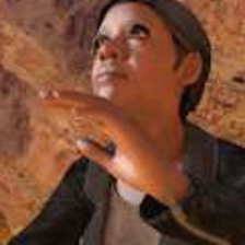
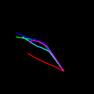
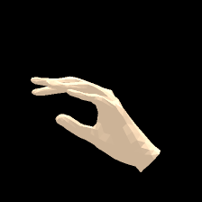
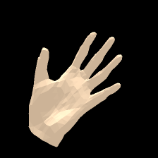
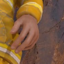
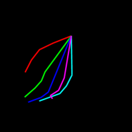
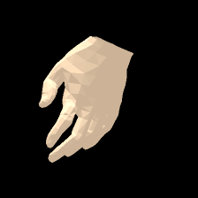
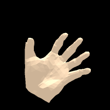
Figure 1: Dense hand pose estimation examples. Our system estimates 3D shapes, as well as articulations and viewpoints. Left to right: input images, coarse skeletal representations, dense hand pose representations, and recovered hand shapes in a canonical articulation/viewpoint. Dense pose estimation provides a richer description of hands and improves the pose estimation accuracy.

Discriminative methods based on convolutional neural networks (CNNs) have shown very promising performance in estimating 3D hand poses either from RGB images [43, 68, 4, 14, 29, 46] or depth maps [65, 30, 50, 58, 30, 64, 28, 38, 64, 2]. However, the predictions are based on coarse skeletal representations, and no explicit kinematics and geometric mesh constraints are often considered. On the other hand, establishing a personalized hand model requires a generative approach that optimizes the hand model to fit to 2D images [40, 33, 36, 51, 49, 48]. Optimization-based methods, besides their complexity, are susceptible to local minima and the personalized hand model calibration contradicts the generalization ability for hand shape variations.

Sinha et al. [45] learn to generate 3D hand meshes from depth images. A direct mapping between a depth map and its 3D surface is learned; however, the accuracy shown is limited. Malik et al. [26] incorporate a 3D hand mesh model to CNNs and learn a mapping between depth maps and mesh model parameters. They further raycast 3D meshes with various viewpoint, shape and articulation parameters to generate a million-scale dataset for training CNNs. Our work tackles the similar but in RGB domain and offers an iterative mesh fitting using a differentiable renderer [18]. This improves once estimated mesh parameters using the gradient information at testing. Our framework also allows indirect 2D supervisions (2D segmentation masks, keypoints) instead of using 3D mesh data.

While 2D keypoint detection is well established in the RGB domain [43], estimating 3D keypoints from RGB images is less trivial. Recently, several methods were developed [68, 34, 4, 14]. While directly lifting 2D estimations to 3D was attempted in [68], 2.5D depth maps are estimated as clues for 3D lifting in state-of-the-art techniques [4, 14]. In this paper, we exploit a deformable 3D hand mesh model, which inherently offers a full description of both hand shapes and articulations, 3D priors for recovering depths, and self-data augmentation. Different from purely generative optimization methods e.g. [34], we propose a method based on a neural renderer and CNNs.

Our contribution is in implementing a full 3D dense hand pose estimator (DHPE) using single RGB images via a neural renderer. Our technical contributions are largely threefold:

1) DHPE is composed of convolutional layers that first estimate 2D evidences (RGB features, 2D keypoints) from an RGB image and then estimate the 3D mesh model parameters. Since RGB/mesh pairs are lacking, the network is learned to fit the 3D model using 2D segmentation masks and skeletons as supervision, similar to recent work on human body pose estimation [57, 16, 35], via neural renderer. The dense shape estimation helps improve the pose estimation.

2) At the testing time, we iteratively refine the initial 3D mesh estimation using the gradients. The gradients are computed over self-supervisions by comparing estimated 3D meshes to predicted 2D evidences, as ground-truth labels are not available at testing. While previous work [57] fixed 2D skeletons/segmentation masks during the refinement step, we recursively improve 2D skeletons and exploit the improved skeletons and feature similarities for 2D masks.

3) To further deal with limited annotated training data, especially for diverse shapes and view-points, we supply fitted meshes and their 2D projected RGB maps by varying shapes and view-points, to fine-tuning the network. Purely synthetic data imposes a synthetic-real domain gap, and annotating 3D meshes or 2D segmentation masks of real images is difficult. Once the model is successfully fitted to input RGB images, its meshes, i.e. shapes and poses are close-to-real.

The proposed method can also be seen as a hybrid method [23, 63, 55] combining merits of discriminative and generative approaches.

2 Related work

Hand pose estimation. There have been several categories of works predicting hand poses. They vary according to types of output (3D mesh, 3D skeletal and 2D skeletal representations) and input (RGB and depth maps).

3D hand model fitting methods. In [54, 53, 41, 51, 49, 48, 40, 33], 3D hand mesh representation is used to describe hand poses. To recover 3D meshes from 2D images, most methods rely on complex optimization methods or use point clouds to fit their 3D mesh models. One recent method [34] takes RGB images as input and formulates the framework that runs in real-time. Their 3D mesh model is matched to estimated 2D skeletons. However, 2D skeleton is coarse and overall 3D fitting fails when the 2D skeleton estimation is not accurate.

Recovering 3D skeletal representations from depth images. Estimating 3D hand skeletons from depth images has shown promising accuracies [64]. The problem is better set since the depth input inherently offers rich 3D information [52]. Further, deep learning methods [65, 30, 50, 58, 30, 64, 28, 38, 64, 2] have been successfully applied along with the million-scale hand pose dataset [65] in this domain. Recently, Malik et al. [26] proposed to estimate both 3D skeletal and mesh representations and have obtained improved accuracy in 3D skeletal estimation. They collect a new million-scale data set for depth map and 3D mesh pairs to train the network in a fully supervised manner.

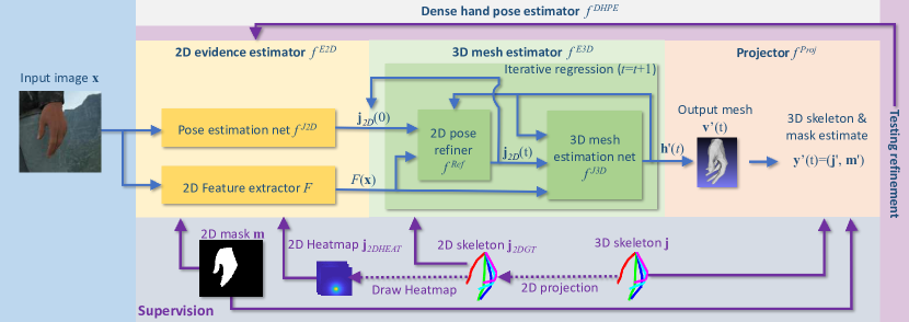
Figure 2: Schematic diagram of the proposed dense hand pose estimation (DHPE) framework. Our DHPE receives an input RGB image $\mathbf{x}$ and estimates the corresponding hand shape and pose as parameters $\mathbf{h}$ of the MANO hand model. Training DHPE is guided via 1) an additional projector $f^{\text{\emph{Proj}}}$ that enables us to provide supervision via 3D skeletons $\mathbf{j}$ and foreground segmentation masks $\mathbf{m}$; 2) decomposing the DHPE into the 2D evidence estimator $f^{\text{\emph{E2D}}}$ and 3D mesh estimator $f^{\text{\emph{E3D}}}$ which stratifies the training via the intermediate 2D feature estimation step. At testing, once the output mesh parameter $\mathbf{h}^{\prime}$ is estimated, it is iteratively refined via enforcing its consistency over intermediate 2D evidences $F(\mathbf{x})$ and $\mathbf{j}_{2D}$.

Estimating the 2D skeletal from RGB. Recovering 2D skeletal representations from RGB images has been greatly improved [43]. Compared to the depth domain, real RGB data is scarce and automatic pose annotation of RGB images still remains challenging. Simon et al. achieved promising results by mixing real data with a large amount of synthetic data [43]. Further accuracy improvement has been obtained by the automatic annotation using label consistency in a multiple camera studio [15].

Recovering the 3D skeletal from RGB. The problem has inherent uncertainties rising from 2D-to-3D mapping [14, 4, 68]. The earlier work [68] attempts to learn the direct mapping from RGB images to 3D skeletons. Recent methods [4, 14] have shown the state-of-the-art accuracy by implicitly reconstructing depth images i.e. 2.5D representations, and estimating the 3D skeletal based on them. We instead use a 3D mesh model in a hybrid way to tackle the problem.

3D representations for hand pose estimation. Different from human face or body, hand poses exhibit a much wider scope of viewpoints, given an articulation and shape. It is hard to define a canonical viewpoint (e.g. a frontal view). To relieve the issue, intermediate 3D representations such as projected point clouds [9], D-TSDF [10], voxels [28] or point sets [8] have been proposed. Though these approaches have shown promising results, they are limited such that they cannot re-generate full 3D information.

3D recovery in other domains. 3D reconstruction has a long history in the field. Some latest approaches using neural networks are discussed below.

3D voxel reconstruction. Voxel representations are useful to describe 3D aspects of objects [62, 56]. Yan et al. [62] proposed a differentiable way to reconstruct voxels given only 2D inputs. Also, Tulsiani et al. [56] proposed a method to use multiple images caputred at different viewpoints to accurately reconstruct voxels. However, the voxel representation is sparse compared to the mesh counterpart. To relieve the issue, a hierarchical method was proposed by Riegler et al. [39].

3D mesh reconstruction. Recently, Güler et al. [11] proposed a way to reconstruct human bodies from RGB inputs. This method requires full 3D supervisions from lots of pairs of 2D images and 3D mesh annotations. Differentiable renderers [25, 18] have been proposed such that 2D silhouettes, depth maps and even textured RGB maps are obtained by projecting 3D models to image planes in a differentiable way. With the use of this renderer, it becomes much easier to reconstruct 3D meshes [17], not needing full 3D supervisions. End-to-end CNN methods with the SMPL model [24] have been proposed for recovering 3D meshes of human bodies [57, 16, 35]. Hands are, however, different from human bodies: hands exhibit much wider viewpoint variations (both egocentric/third-person views), highly articulated and frequently occluded joints. Also, there are relatively fewer full 3D annotations of RGB images available. These domain differences make the naïve application of the existing methods to this domain non-optimal.

3 Proposed dense hand pose estimator

Our goal is to construct a hand mesh estimator (HME) $f^{\text{\emph{HME}}}:\mathcal{X}\to\mathcal{V}$ that maps an input RGB image $\mathbf{x}\in\mathcal{X}$ to the corresponding estimated 3D hand mesh $\mathbf{v}\in\mathcal{V}$. Each input is given as an RGB pixel array of size 224$\times$224 while an output mesh corresponds to 3D positions of 778 vertices encoding 1,538 triangular faces. Instead of directly generating a mesh $\mathbf{v}$ as a $778\times 3$-dimensional raw vector, our HME estimates a 63-dimensional parameter vector $\mathbf{h}$ that represents $\mathbf{v}$ by adopting the MANO 3D hand mesh model [41] (Sec. 3.2). Once a hand mesh $\mathbf{v}$ (or equivalently, its parameter $\mathbf{h}$) is estimated, the corresponding skeletal pose $\mathbf{j}$ consisting of 21 3D joint positions can be recovered via a 3D skeleton regressor $f^{\text{\emph{Reg}}}$ discussed shortly.

Learning the HME can be cast into a standard multivariate regression problem if a training database of pairs of input images and the corresponding ground-truth meshes are available. However, we are not aware of any existing database that provides such pairs. Inspired by the success of existing human body reconstruction work [57, 16, 35], we take an indirect approach by learning a dense hand pose estimator (DHPE) which combines the HME and a new projection operator. The projection operator consists of a 3D skeleton regressor and a renderer which respectively recover a 3D skeletal pose ($\mathbf{j}\in\mathcal{J}$) and a 2D foreground hand segmentation mask ($\mathbf{m}\in\mathcal{M}$) from a hand mesh $\mathbf{v}$. Table 1 shows our notation, and Eq. 1 and Fig. 2 summarize the decomposition of DHPE:

$$\mathcal{X}\underbrace{\overbrace{\xrightarrow{f^{\text{\emph{E2D}}}}\mathcal{Z}\xrightarrow{f^{\text{\emph{E3D}}}}}^{f^{\text{\emph{HME}}}=f^{\text{\emph{E3D}}}\circ f^{\text{\emph{E2D}}}}\mathcal{V}\xrightarrow{f^{\text{\emph{Proj}}}=(f^{\text{\emph{Reg}}},f^{\text{\emph{Ren}}})}}_{f^{\text{\emph{DHPE}}}=f^{\text{\emph{Proj}}}\circ f^{\text{\emph{HME}}}}\mathcal{Y}=(\mathcal{J},\mathcal{M}).$$ (1)

Table 1: Notational summary

$\mathbf{y}$	$\mathbf{y}=(\mathbf{j},\mathbf{m})\in\mathcal{Y}=(\mathcal{J},\mathcal{M})\subset\mathbb{R}^{(21\times 3)\times(224\times 224)}$
$f^{\text{\emph{DHPE}}}$	dense hand pose estimator ($f^{\text{\emph{DHPE}}}=f^{\text{\emph{Proj}}}\circ f^{\text{\emph{HME}}}$)
$f^{\text{\emph{Proj}}}$	projection operator ($f^{\text{\emph{Proj}}}=[f^{\text{\emph{Reg}}},f^{\text{\emph{Ren}}}]$)
$f^{\text{\emph{Reg}}}$	3D skeleton regressor
$f^{\text{\emph{Ren}}}$	renderer

Extending the skeleton regressor provided by the MANO model [41], our skeleton regressor $f^{\text{\emph{Reg}}}$ maps a hand mesh $\mathbf{v}$ to its skeleton $\mathbf{j}$ consisting of 21 3D joint positions. It is a linear regressor implemented as three matrices of size $778\times 21$ (see Sec. 2.1 of the supplemental for details).

Our renderer $f^{\text{\emph{Ren}}}$ generates the foreground hand mask $\mathbf{m}$ by simulating the camera view of $\mathbf{x}$. We adopt the differentiable neural renderer proposed by Kato et al. [18].

By construction, the projection operator respects the underlying camera (via $f^{\text{\emph{Ren}}}$) and hand shape (via $f^{\text{\emph{Reg}}}$) geometry and it is held fixed throughout the entire training process. This facilitates the training of $f^{\text{\emph{HME}}}$ indirectly via training $f^{\text{\emph{DHPE}}}$. However, even under this setting, the problem still remains challenging as estimating a 3D mesh given an RGB image is a seriously ill-posed problem. Adopting recent human body pose estimation approaches [35, 57], we further stratify learning of $f^{\text{\emph{DHPE}}}:\mathcal{X}\to\mathcal{Y}$ by decomposing $f^{\text{\emph{HME}}}:\mathcal{X}\to\mathcal{V}$ into a 2D evidence estimator $f^{\text{\emph{E2D}}}:\mathcal{X}\to\mathcal{Z}$ and a 3D mesh estimator $f^{\text{\emph{E3D}}}:\mathcal{Z}\to\mathcal{V}$. Our 2D evidence $\mathbf{z}\in Z$ consists of a 42-dimensional 2D skeletal joint position vector $\mathbf{j}_{2D}$ (21 positions $\times$ 2; as in [4, 14]) and a 2,048-dimensional 2D feature vector $F(\mathbf{x})$ (Eq. 2). The remainder of this section provides details of these two estimators.

3.1 2D evidence estimator $f^{\text{\emph{E2D}}}=(F,f^{\text{\emph{J2D}}})$

Silhouettes (or foreground masks) and 2D skeletons have been widely used as the mid-level cues for estimating 3D body meshes [17, 35, 57]. However, for hands, accurately estimating foreground masks from RGB images is challenging due to cluttered backgrounds [21, 68]. We observed that naïvely applying the state-of-the-art foreground segmentation algorithms (e.g. [68]) often misses fine details, especially along the narrow finger regions (see Fig. 4 for examples) and this can significantly degrade the performance of the subsequent mesh estimation step. We bypass this challenge by learning instead, a 2D foreground feature extractor $F$: $F(\mathbf{x})$ encapsulates the textural and shape information of the foreground regions in $\mathbf{x}$.

Our 2D feature extractor $F$ is trained to focus on the foreground regions by minimizing the deviation between the features extracted from the entire image $\mathbf{x}$ and the foreground region $\mathbf{x}\odot\mathbf{m}$ extracted via the ground-truth mask $\mathbf{m}$ (see Fig. 3d): The training loss (per data point) for $F$ is given as

$$L_{\text{\emph{Feat}}}(F)=\|F(\mathbf{x})-F(\mathbf{x}\odot\mathbf{m})\|^{2}_{2},$$ (2)

where $\odot$ denotes element-wise multiplication. $F$ employs the ResNet-50 [13] architecture whose output is a 2,048-dimensional vector.

() (a)

() (b)

() (c)

() (d)

Figure 3: A 2D evidence estimation example. (a) input image $\mathbf{x}$, (b) ground-truth 2D segmentation mask $\mathbf{m}$ of $\mathbf{x}$, (c) 2D skeletal position heat map of the finger tip of middle finger overlaid on $\mathbf{x}$, and (d) masked image $\mathbf{x}\odot\mathbf{m}$.

Estimating 2D skeletal joints from an RGB image has been well studied. Similarly to [4, 14], we embed the state-of-the-art 2D pose estimation network $f^{\text{\emph{J2D}}}$ [60, 68] into our framework. The initial weights provided by the authors of  [68] are refined based on the 2D joint estimation loss:

$$L_{\text{\emph{J2D}}}(f^{\text{\emph{J2D}}})=\|f^{\text{\emph{J2D}}}(\mathbf{x})-\mathbf{j}_{\text{\emph{2DHeat}}}\|^{2}_{2}.$$ (3)

The output of $f^{\text{\emph{J2D}}}$ is a matrix of size 21$\times$32$\times$32 encoding 21 heat maps (per joint) of size 32$\times$32. $\mathbf{j}_{\text{\emph{2DHeat}}}$ is the ground-truth heat map. Given the estimated heat maps, 2D skeleton joints $\mathbf{j}_{\text{\emph{2D}}}$ are extracted by finding the maximum for each joint. Figure 3(b) shows an example of 2D evidence estimation.

3.2 3D mesh estimator $f^{\text{\emph{E3D}}}=(f^{\text{\emph{J3D}}},f^{\text{\emph{Ref}}})$

Taking the 2D evidence $\mathbf{z}$ ($2,048$-dimensional feature vector $F(\mathbf{x})$ and $21\times 3$-dimensional 2D skeleton $\mathbf{j}_{\text{\emph{2D}}}$) as input, the 3D mesh estimation network $f^{\text{\emph{J3D}}}$ constructs parameters of a deformable hand mesh model and a camera model. We use the MANO model representing a hand mesh based on 45-dimensional pose parameters $\mathbf{p}$ and 10-dimensional shape parameters $\mathbf{s}$ [41]. The original MANO framework uses only 6-dimensional (principal component analysis) PCA subspace of $\mathbf{p}$ for computational efficiency. However, we empirically observed that to cover a variety of hand poses, all 45-dimensional features are required: We use the linear blend skinning formulation as in the SMPL model [24].

Given the MANO parameters $\mathbf{p}$ and $\mathbf{s}$, a mesh $\mathbf{v}$ is synthesized by conditioning them on the hypothesized camera $\mathbf{c}$, which comprises of the 3D rotation (in quaternion space) $\mathbf{c}_{q}\in\mathbb{R}^{4}$, scale $\mathbf{c}_{s}\in\mathbb{R}$, and translation $\mathbf{c}_{t}\in\mathbb{R}^{3}$: An initial mesh is constructed by combining MANO’s PCA basis vectors using the shape parameter $\mathbf{s}$, rotating the bones according to the pose parameter $\mathbf{p}$, and deforming the resulting surface via linear blend skinning. The final mesh $\mathbf{v}$ is then obtained by globally rotating, scaling, and translating the initial mesh according to $\mathbf{c}_{q}$, $\mathbf{c}_{s}$, and $\mathbf{c}_{t}$, respectively. The entire mesh generation process is differentiable. Under this model, our 3D mesh estimation network $f^{\text{\emph{J3D}}}$ is implemented as a single fully-connected layer of 2153$\times$63 weights and it estimates a 63-dimensional mesh parameter:

$$\mathbf{h}=[\mathbf{p},\mathbf{s},\mathbf{c}_{q},\mathbf{c}_{s},\mathbf{c}_{t}]^{\top}.$$ (4)

Iterative mesh refinement via back-projection. Adopting Kanazawa et al.’s approach [16], instead of estimating $\mathbf{h}$ directly, we iteratively refine the initial mesh estimate $\mathbf{h}(0)$ by recursively performing regression on the parameter offset $\Delta\mathbf{h}$: At iteration $t$, $f^{\text{\emph{J3D}}}$ takes $\mathbf{z}$ and the current mesh estimate $\mathbf{h}(t)$, and generates a new offset $\Delta\mathbf{h}(t)$:

$$\mathbf{h}(t+1)=\mathbf{h}(t)+\Delta\mathbf{h}(t).$$ (5)

At $t=0$, $\mathbf{h}(0)$ as an input to $f^{\text{\emph{J3D}}}$, is constructed as a vector of zeros except for the entries corresponding to the pose parameter $\mathbf{p}$ which is set as the mean pose of the MANO model. We fix the number of iterations at 3 as more iterations did not show any noticeable improvements in preliminary experiments.

In [16], each offset prediction $\Delta\mathbf{h}(t)$ is built based only on 2D features $F(\mathbf{x})$. Inspired by the success of [4, 14], we additionally use 2D skeletal joint $\mathbf{j}^{\prime}_{2D}$ as input. However, as an estimate, $\mathbf{j}^{\prime}_{2D}(0)$ (obtained at iteration $0$) is inaccurate, causing errors in the resulting $\Delta\mathbf{h}(t)$ estimate. Then, these errors accumulate over iterations (Eq. 5) lessening the benefit of the entire iterative estimation process. We address this by an additional 2D pose refiner $f^{\text{\emph{Ref}}}$ which iteratively refines the 2D joint estimation $\mathbf{j}^{\prime}_{2D}(t)$ via back-projecting the estimated mesh $\mathbf{h}^{\prime}(t)$: At $t$, $f^{\text{\emph{Ref}}}$ receives the estimated mesh parameter $\mathbf{h}^{\prime}(t)$, 2D feature $F(\mathbf{x})$, 3D skeleton $f^{\text{\emph{Reg}}}(\mathbf{v}^{\prime})$, and $\mathbf{j}^{\prime}_{2D}(t)$, and generates a refined estimate $\mathbf{j}^{\prime}_{2D}(t+1)$. The 2D pose refiner $f^{\text{\emph{Ref}}}$ is implemented as a single fully connected layer of size 2216$\times$42 and it is trained based on the ground-truth 2D skeletons ($\mathbf{j}_{\text{\emph{2DGT}}}$):

$$L_{\text{\emph{Ref}}}=\left\|f^{\text{\emph{Ref}}}\left([\mathbf{j}^{\prime}_{2D}(t),F(\mathbf{x}),\mathbf{h}^{\prime}(t),f^{\text{\emph{Reg}}}(\mathbf{v}^{\prime})]\right)-\mathbf{j}_{\text{\emph{2DGT}}}\right\|^{2}_{2}.$$ (6)

In the experiments, we demonstrate that 1) using both 2D features and 2D skeletons (Fig. 5(e): ‘Ours (w/o Test. ref. and Refiner $f^{\text{\emph{Ref}}}$)’) improves performance over Kanazawa et al.’s 2D feature-based framework [16] (Fig. 5(e): ‘Ours (w/o Test. ref., $f^{\text{\emph{Ref}}}$ and 2D losses ($L_{Feat}$, $L_{J2D}$)’); 2) explicitly building the refiner $f^{\text{\emph{Ref}}}$ under the auxiliary 2D joint supervision (Fig. 5(e): ‘Ours (w/o Test. ref.)’) further significantly improves performance. More importantly, the refiner takes a crucial role in our testing refinement step (Sec. 3.4) which improves a once predicted 3D mesh $\mathbf{v}^{\prime}$ by enforcing its consistency with the corresponding 2D joint evidence $\mathbf{j}^{\prime}_{\text{\emph{2D}}}(t)$ (as well as other intermediate results) throughout the iteration (Eq. 13).

3.3 Joint training

Training the 2D evidence estimator $f^{\text{\emph{E2D}}}:\mathcal{X}\to\mathcal{Z}$ and 3D mesh estimator $f^{\text{\emph{E3D}}}:\mathcal{Z}\to\mathcal{V}$ given fixed projection operator $f^{\text{\emph{Proj}}}:\mathcal{V}\to\mathcal{Y}$ is performed based on a training set consisting of input images, and the corresponding 3D skeleton joints and 2D segmentation masks $D=\{(\mathbf{x}_{i},\mathbf{y}_{i}\}_{i=1}^{l}\subset\mathcal{X}\times\mathcal{Y}$, $\mathbf{y}_{i}=(\mathbf{j}_{i},\mathbf{m}_{i})$. Since all component functions of $f^{\text{\emph{E2D}}}$, $f^{\text{\emph{E3D}}}$, and $f^{\text{\emph{Proj}}}$ are differentiable with respect to the weights of $F$ and $f^{\text{\emph{E3D}}}$, they can be optimized based on on standard gradient descent-type algorithm: Our overall loss (per training instance $\mathbf{x}_{i},\mathbf{y}_{i}$) is given as (see Eqs. 2 and 6):

$$L(f^{\text{\emph{E3D}}},F) =L_{\text{\emph{Art}}}(f^{\text{\emph{E3D}}},F)+L_{\text{\emph{Lap}}}(f^{\text{\emph{E3D}}},F)+L_{\text{\emph{Feat}}}(F)$$

$$+\lambda L_{\text{\emph{Sh}}}(f^{\text{\emph{J3D}}},F)+L_{\text{\emph{Ref}}}(f^{\text{\emph{J3D}}},F).$$ (7)

The articulation loss $L_{\text{\emph{Art}}}$ measures the deviation between the skeleton estimated from $\mathbf{x}_{i}$ and its ground-truth $\mathbf{j}_{i}$:

$$L_{\text{\emph{Art}}}=\|[f^{\text{\emph{DHPE}}}(\mathbf{x}_{i})]_{\mathcal{J}}-\widehat{\mathbf{j}_{i}}\|^{2}_{2},$$ (8)

where $[\mathbf{y}]_{\mathcal{J}}$ extracts the $\mathbf{j}$-component of $\mathbf{y}=(\mathbf{j},\mathbf{m})$ and $\widehat{\mathbf{j}}$ spatially normalizes $\mathbf{j}$ similarly to [14, 68]: First, the center of each skeleton is moved to the corresponding middle finger’s MCP position. Then each axis is normalized to a unit interval $[0,1]$: The $x,y-$coordinate values are divided by $g$ (=1.5 times the maximum of height and width of the tight 2D hand bounding box). The $z-$axis value is divided by $(z_{\text{\emph{Root}}}\times g)/\mathbf{c}_{f}$ where $z_{\text{\emph{Root}}}$ is the depth value of the middle finger’s MCP joint and $\mathbf{c}_{f}$ is the focal length of the camera. At testing, once normalized skeletons are estimated, they are inversely normalized to the original scale. The accompanying supplemental provides details of this inverse normalization step.

Our shape loss $L_{\text{\emph{Sh}}}$ facilitates the recovery of hand shapes as observed indirectly via projected 2D segmentation masks:

$$L_{\text{\emph{Sh}}}=\left\|[f^{\text{\emph{DHPE}}}(\mathbf{x}_{i})]_{\mathcal{M}}-\mathbf{m}_{i}\right\|^{2}_{2},$$ (9)

where $[\mathbf{y}]_{\mathcal{M}}$ extracts the $\mathbf{m}$-component of $\mathbf{y}=(\mathbf{j},\mathbf{m})$.

The Laplacian regularizer $L_{\text{\emph{Lap}}}$ enforces spatial smoothness in the mesh $\mathbf{v}$. This helps avoid generating implausible hand meshes as suggested by Kanazawa et al. [17].

Hierarchical recovery of articulation and shapes. We observed that naïvely minimizing the overall loss $L$ with a constant shape loss weight $\lambda$ (Eq. 7) tends to impede convergence during training (Fig. 5(f)): Our algorithm simultaneously optimizes the mesh ($\mathbf{v}$) and camera ($\mathbf{c}=\{\mathbf{c}_{q},\mathbf{c}_{s},\mathbf{c}_{t}\}$) parameters which over-parameterize the rendered 2D view, e.g. the effect of scaling $\mathbf{v}$ itself can be offset by inversely scaling $\mathbf{c}_{s}$. This often hinders the alignment of $\mathbf{v}$ with the ground-truth 2D mask and thereby rendering the network inappropriately update the mesh parameters. Therefore, we let the shape loss $L_{\text{\emph{Sh}}}$ take effect only when the articulation loss $L_{\text{\emph{Art}}}$ becomes sufficiently small: $\lambda$ is set per data instance based on the $L_{\text{\emph{Art}}}$-value:

$$\lambda=\left\{\begin{array}[]{ll}1&\textrm{if $\left\|\left[[f^{\text{\emph{DHPE}}}(\mathbf{x}_{i})]_{\mathbf{j}}\right]_{2D}-[\mathbf{j}_{i}]_{2D}\right\|^{2}_{2}<\tau$}\\ 0&\textrm{otherwise},\end{array}\right.$$ (12)

where $[\mathbf{j}]_{2D}$ projects 3D joint coordinates $\mathbf{j}$ to 2D view based on $\mathbf{c}$ (Eq. 4). The threshold $\tau$ is empirically set to $15$ pixels. Initially, with zero $\lambda$, $L_{\text{\emph{Art}}}$ dominates in $L$, which helps globally align the estimated meshes with 2D ground-truth evidence. As the training progresses, the role of $L_{\text{\emph{Sh}}}$ becomes more important ($\lambda=1$) contributing to recovering the detailed shapes.

As the generation of the 2D skeleton $\mathbf{j}_{\text{\emph{2D}}}$ from an estimated heat-map $f^{\text{\emph{J2D}}}(\mathbf{x})$ is not differentiable (see Eq. 3), our 2D pose estimation network $f^{\text{\emph{J2D}}}$ cannot be trained based on $L$. Thus we train it in parallel using $L_{\text{\emph{J2D}}}$ (Eq. 3). For both cases, we use the standard Adam optimizer with the learning rate $\gamma$ set at $10^{-3}$.

3.4 Testing refinement

To facilitate the training of the HME, we constructed an auxiliary DHPE that decomposes into three component functions: $f^{\text{\emph{Proj}}}$, $f^{\text{\emph{E2D}}}$, and $f^{\text{\emph{E3D}}}$ (see Eq. 1). An important benefit of this step-wise estimation approach is that it enables us to check and improve once predicted output mesh by comparing it with the intermediate results: For testing, the underlying mesh $\mathbf{v}$ of a given test image $\mathbf{x}$ can be first estimated by applying $f^{\text{\emph{HME}}}=f^{\text{\emph{E3D}}}\circ f^{\text{\emph{E2D}}}:\mathcal{X}\to\mathcal{V}$. If the resulting prediction $\mathbf{v}^{\prime}$ (equivalently, $\mathbf{h}^{\prime}$) is accurate, it must be in accordance with the intermediate results $F(\mathbf{x})$ and $\mathbf{j}_{\text{\emph{J2D}}}^{\prime}$ generated from $\mathbf{x}$. Checking and further enforcing this consistency can be facilitated by noting that our loss function $L$ and its components are differentiable with respect to the mesh parameter $\mathbf{h}$. By reinterpreting $L$ as a smooth function of $\mathbf{h}$ given fixed $f^{\text{\emph{Proj}}}$, $f^{\text{\emph{E2D}}}$, and $f^{\text{\emph{E3D}}}$, we can refine the initial prediction $\mathbf{h}^{\prime}(0)$ by enforcing such consistency:

$$\mathbf{h}^{\prime}(t+1) =\mathbf{h}^{\prime}(t)-\gamma\cdot\nabla_{\mathbf{h}}\Big{(}\left\|\left[[f^{\text{\emph{DHPE}}}(\mathbf{x})]_{\mathcal{J}}\right]_{XY}-{\mathbf{j}^{\prime}}_{\text{\emph{J2D}}}\right\|^{2}_{2}$$

$$+\lambda\left\|F(\mathbf{x})-F(f^{\text{\emph{Ren}}}(\mathbf{v}^{\prime})\odot\mathbf{x})\right\|^{2}_{2}+L_{\text{\emph{Lap}}}\Big{)},$$ (13)

where $[\mathbf{j}]_{XY}$ extracts the $x,y-$coordinate values of skeleton joints from $\mathbf{j}$. Note that in the first gradient term, we use the 2D skeleton ${\mathbf{j}^{\prime}}_{\text{\emph{2D}}}$ since the ground-truth 3D skeleton $\widehat{\mathbf{j}}$ is not available at testing. This step benefits from explicitly building the 2D pose refiner $f^{\text{\emph{Ref}}}$ that improves the once estimated 2D joint ${\mathbf{j}^{\prime}}_{\text{\emph{2D}}}$ during iterative mesh estimation process (Eq. 5). Also, for the second, shape loss term of the gradient, since the ground-truth segmentation mask $\mathbf{m}$ is not available, we use the segmentation mask rendered via $f^{\text{\emph{Ren}}}$ based on the estimated mesh $\mathbf{v}^{\prime}$ enforcing self-consistency. The number of iterations in Eq. 13 is fixed at 50. Our testing refinement step takes 250ms (5ms per iteration $\times$ 50 iterations) in addition to the initial regression step which takes 100ms. Figure 5(e) shows the performance variation with varying number of iterations.

3.5 Self-supervised data augmentation

An important advantage of incorporating a generative mesh model (i.e. MANO) into the training process of the HME (via $\mathbf{h}$; see Eq. 4) is that it can synthesize new data as guided by (and subsequently, guiding) HME. The MANO model provides explicit control over the shape of synthesized 3D hand mesh. Combining this with a camera model, we can generate pairs of 3D meshes, and the corresponding rendered 2D masks and RGB images.

To render RGBs, we adopt the neural texture renderer $f^{\text{\emph{TRen}}}$ proposed by Kato et al. [18]: During training, once a seed mesh $\mathbf{v}^{S}$ is predicted, the corresponding camera and shape parameters $\mathbf{h}^{S}$ are changed to generate new meshes $\{\mathbf{v}^{\text{\emph{N}}}_{j}\}$: The shape parameter $\mathbf{s}$ is sampled uniformly from the interval covering three times the standard deviation per dimension. For camera perspectives, the rotation matrix along each of $x,y,z-$ axes are sampled uniformly on $[0,2\pi]$. Once the foreground hand region is rendered via $f^{\text{\emph{TRen}}}$, it is placed on random backgrounds obtained from the NYU depth database [42].

For each new mesh $\mathbf{v}^{\text{\emph{N}}}$, we generate a triplet $\left(f^{\text{\emph{TRen}}}(\mathbf{v}^{\text{\emph{N}}}),f^{\text{\emph{Ren}}}(\mathbf{v}^{\text{\emph{N}}}),f^{\text{\emph{Reg}}}(\mathbf{v}^{\text{\emph{N}}})\right)$ constituting a new training instance for the DHPE. We empirically observed that when the training of the DHPE reaches $20$ epochs, it tends to generate seed meshes $\{\mathbf{v}^{S}_{i}\}$ which faithfully represent realistic hand shapes (even though they might not accurately match the corresponding input images $\{\mathbf{x}_{i}\}$). Therefore, we initiate the augmentation process after the first $20$ training epochs. For each mini-batch, three new data instances are generated per seed prediction $\mathbf{v}^{S}$ gradually enlarging the entire training set (see supplemental for examples). A similar self-supervised data augmentation approach has been adopted for facial shape estimation [22].

()

()

()

()

()

()

()

()

Figure 4: Hand segmentation examples. Left to right: input images, ground-truth masks, our results, the results of the state-of-the-art hand segmentation algorithm [21].

4 Experiments

Experimental settings.

We evaluate the performance of our algorithm on 3 hand pose estimation datasets. Stereo hand pose dataset (SHD) provides frames of 12 stereo video sequences each recording a single person performing various gestures  [66]. It contains total 36,000 frames. Among them, 30,000 frames sampled from 10 videos constitute a training set while the remaining 6,000 frames (from 2 videos) are used for testing. The rendered hand pose dataset (RHD) contains 43,986 synthetically generated images showing 20 different characters performing 39 actions where 41,258 images are provided for training while the remaining 2,728 frames are reserved for testing [68]. Both datasets are recorded under varying backgrounds and lighting conditions and they are provided with the ground-truth 2D and 3D skeleton positions of 21 keypoints (1 for palm and 4 for each finger), on which the accuracy is measured. The Dexter+Object dataset (DO) contains 3,145 video frames sampled from 6 video sequences recording a single person interacting with an object (see Fig. 6(DO)) [47]. This dataset provides ground-truth 3D skeleton positions for the 5 finger-tips of the left hand: The overall accuracy is measured in these finger-tip locations. Following the experimental settings in [68, 4, 14] we train our system on 71,258 frames combining the original training sets of SHD and RHD. For testing, the remaining frames in SHD and RHD, respectively and the entire DO is used. The overall hand pose estimation accuracy is measured in the area under the curve (AUC) and the ratio of correct keypoints (PCK) with varying thresholds for each [68, 4, 14].

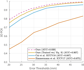
() Accuracies on RHD

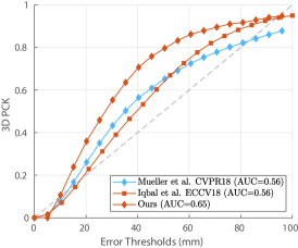
() Accuracies on DO

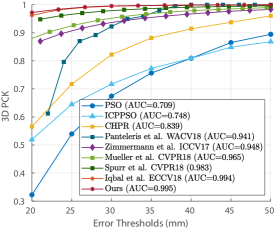
() Accuracies on SHD

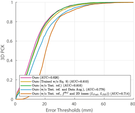
() Ablation study results RHD

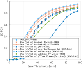
() Ablation study results DO

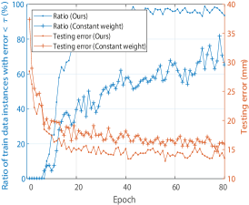
() Progression of the DHPE accuracies

Figure 5: Performances of different algorithms on three benchmark datasets: (a-c) accuracies on RHD, DO, and SHD, respectively; (d-e) evaluation of our algorithm design choices on RHD and DO, respectively; (f) progressions of the testing errors (orange curves) and the ratio of training data instances with small joint estimation errors ($<\tau$ in Eq. 12; blue curves) with $\lambda$ fixed at $0.01$ (curves with dot markers) and with $\lambda$ scheduled based on Eq. 12 (curves with cross markers).

Table 2: Performances of different hand segmentation algorithms on RHD (higher is better).

Method	IOU score	Precision	Recall	F1-score
Ours	$65.13\%$	$82.82\%$	$75.31\%$	$78.88$
[68]	$35.40\%$	$36.52\%$	$92.06\%$	$52.29$
[21]	$52.68\%$	$71.65\%$	$66.55\%$	$69.00$

For comparison, we adopt seven hand pose estimation algorithms including five neural networks (CNNs)-based algorithms ([4, 68] for RHD, [14, 29] for DO, and [29, 68, 46] for SHD) and two 3D model fitting-based algorithms [34, 19].

Many existing CNN-based algorithms guide the learning process via building intermediate 2D evidence: Zimmermann and Brox’s algorithm [68] first estimates 2D skeletons from the input RGB images and thereafter, maps estimated 2D skeletons to 3D skeletons. Spurr et al.’s algorithm [46] builds a latent space shared by RGB images and 2D/3D skeletons. Cai et al.’s algorithm [4] trains an RGB-to-depth synthesizer that generates intermediate depth-map estimates to guide skeleton estimation. Similarly, Iqbal et al.’s algorithm [14] reconstructs depth maps from input RGB images. Unlike these algorithms, our algorithm builds full 3D meshes to guide the skeleton estimation process.

Mueller et al. [29] approached the challenge of building realistic training data pairs of 3D skeletons and RGB images by first generating synthetic RGB images from skeletons and then transferring these images into realistic ones via a GAN transfer network. On the other hand, our algorithm focuses on dense hand pose estimation and thus it generates pairs of RGB images and the corresponding 3D meshes.

Results. Figure 5 summarizes the results. Our algorithm improved Zimmermann and Brox’s algorithm [68] with a large margin (Fig. 5(a)). Also, a significant accuracy gain ($\approx$4mm on average) from Cai et al.’s approach [4] was obtained, demonstrating the effectiveness of our 3D mesh-guided supervision in comparison to 2.5D depth map-guided supervision. Figure 5(a) also demonstrates that jointly estimating the shape and pose (using Eqs. 8 and 9) leads to higher pose estimation accuracy than estimating only the pose. Figure 5(b) (DO) shows that our algorithm clearly outperforms [14, 29]: It should be noted that the comparison with [29] is not fair since their networks were trained on a database tailored for object interaction scenarios as in DO. Figure 5(c) (SHD) further demonstrates that in comparison to the state-of-the-art CNN-based algorithms [29, 68, 46] as well as 3D model fitting approaches (PSO and [34]), our algorithm achieves significant performance improvements. The superior performance of our algorithm over [29] shows the effectiveness of our data generation approach. The performance of our algorithm is on par with [14] on this dataset but ours outperforms [14] on DO.

Ablation study. Figure 5(d-e) shows the result of varying design choices in our algorithm on DO and RHD: The testing refinement step (Sec. 3.4) had a significant impact on the final performance: The results obtained without this step (‘w/o Test. ref.’) is considerably worse on DO; On RHD, results of ‘w/o Test. ref.’ are similar. Our data augmentation strategy (Sec. 3.5) further significantly improved the accuracy over ‘w/o Data Aug.’ cases. Figure 5(d-e) further show that explicitly providing supervision to our 2D evidence estimator via 2D losses ($L_{J2D}$ and $L_{Feat}$; Eqs. 2-3) constantly improve the overall accuracy over ‘w/o 2D loss’ cases which correspond to Kanazawa et al.’s iterative estimation framework [16]. Figure 5(f) visualizes the effectiveness of our hierarchical shape and articulation optimization strategy (Eq. 12): In comparison to the case of constant $\lambda$ value (‘Constant weight’), automatically scheduling $\lambda$ based on Eq. 12 led to larger fraction of training instances that have small articulation errors ($<\tau$; Eq. 12) which then led to faster decrease of test error.

Qualitative evaluation. For qualitative evaluation, we show example dense estimation results in Fig. 6. Figure 6(RHD) demonstrates the importance of the shape loss $L_{\text{\emph{Sh}}}$ (Eq. 9) conforming the quantitative results of Fig. 5(a,d).

Hand segmentation performance. Systematically evaluating the performance of dense hand pose estimation (including shape) is challenging due to the lack of ground-truth labels. Therefore, we assess the performance indirectly based on the 2D hand segmentation accuracy. Table 2 shows the results measured in 4 different object segmentation performance criteria. In comparison to the state-of-the-art hand segmentation networks [21, 68] (note [21] is fine-tuned for RHD), our algorithm led to significantly higher accuracy. Also, Fig. 4 shows that the state-of-the-art segmentation net [21] is distracted by other skin colored objects than hands (e.g. arms) while our algorithm, by explicitly estimating 3D meshes, can successfully disregarded these distracting backgrounds.

()

()

()

()

()

()

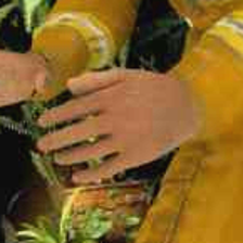
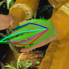
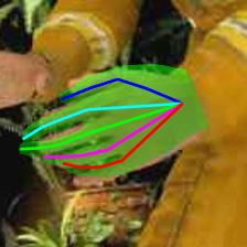
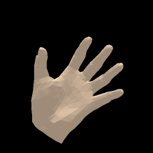
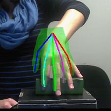
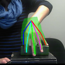
() (ii)

()

()

()

()

()

()

()

()

()

()

()

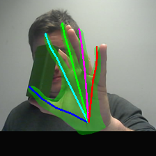
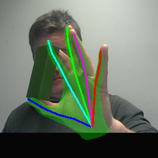
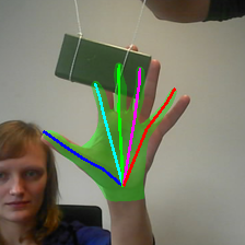
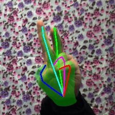
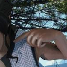
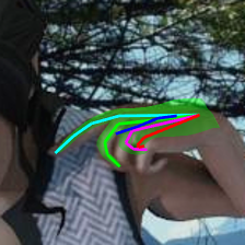
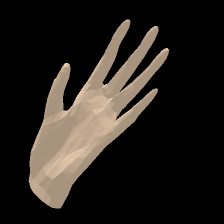
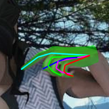
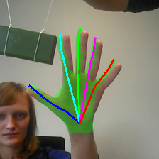
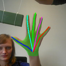
() a

()

()

()

()

()

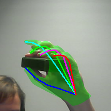
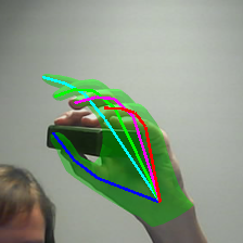
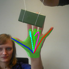
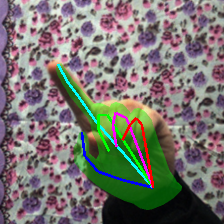
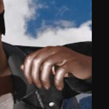
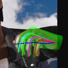
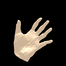
[(a)] [(b)] [(c)] [(d)]

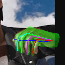
() (RHD)

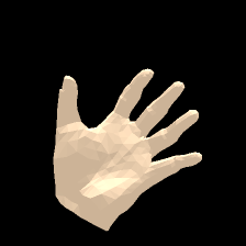
() (e)

[(a)] [(b)] [(c)] [(d)] [(e)]

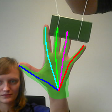
() (DO)

[(a)] [(b)]

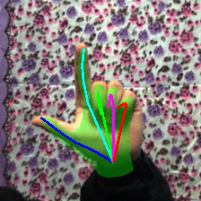
() (SHD)

Figure 6: Example dense hand pose estimation results. (RHD): (a) input images; (b-c) and (d-e) our results obtained without and with the shape loss $L_{\text{\emph{Sh}}}$ (Eq. 9), respectively; (b,d) dense hand pose estimation results, and (c,e) estimated shapes in canonical hand pose. (DO): (a,c) and (b,d) our results obtained without testing refinement and after applying $20$ iterations of testing refinement, respectively; (e) failure and success cases under occlusion. (SHD): (a-b) input images and our results.

5 Conclusions

We have presented dense hand pose estimation (DHPE) network, a CNN-based framework that reconstructs 3D hand shapes and poses from single RGB images. DHPE decomposes into the 2D evidence estimator, 3D mesh estimator and projector. The projector, via the neural renderer, replaces insufficient full 3D supervision with indirect supervision by 2D segmentation masks/3D joints, and enables generating new data. In the experiments, we have demonstrated that stratifying 2D/3D estimators improves accuracy, updating 2D skeletons helps self-supervision in the iterative testing refinement and improves 3D skeleton estimation, and jointly estimating 3D hand shapes and poses offers the state-of-the-art accuracy in both 3D hand skeleton estimation and 2D hand segmentation tasks.

References

- [1] Seungryul Baek, Kwang In Kim, and Tae-Kyun Kim. Real-time online action detection forests using spatio-temporal contexts. In WACV, 2017.
- [2] Seungryul Baek, Kwang In Kim, and Tae-Kyun Kim. Augmented skeleton space transfer for depth-based hand pose estimation. In CVPR, 2018.
- [3] Seungryul Baek, Zhiyuan Shi, Masato Kawade, and Tae-Kyun Kim. Kinematic-layout-aware random forests for depth-based action recognition. In BMVC, 2017.
- [4] Yujun Cai, Liuhao Ge, Jianfei Cai, and Junsong Yuan. Weakly-supervised 3d hand pose estimation from monocular rgb images. In ECCV, 2018.
- [5] Tzu-Yang Chen, Pai-Wen Ting, Min-Yu Wu, and Li-Chen Fu. Learning a deep network with spherical part model for 3D hand pose estimation. In ICRA, 2017.
- [6] Chiho Choi, Sang Ho Yoon, Chin-Ning Chen, and Karthik Ramani. Robust hand pose estimation during the interaction with an unknown object. In ICCV, 2017.
- [7] Guillermo Garcia-Hernando, Shanxin Yuan, Seungryul Baek, and Tae-Kyun Kim. First-person hand action benchmark with RGB-D videos and 3D hand pose annotations. In CVPR, 2018.
- [8] Liuhao Ge, Yujun Cai, Junwu Weng, and Junsong Yuan. Hand PointNet: 3D hand pose estimation using point sets. In CVPR, 2018.
- [9] Liuhao Ge, Hui Liang, Junsong Yuan, and Daniel Thalmann. Robust 3D Hand pose estimation in single depth images: from single-view CNN to multi-view CNNs. In CVPR, 2016.
- [10] Liuhao Ge, Hui Liang, Junsong Yuan, and Daniel Thalmann. 3D convolutional neural networks for efficient and robust hand pose estimation from single depth images. In CVPR, 2017.
- [11] Rıza Alp Güler, Natalia Neverova, and Iasonas Kokkinos. DensePose: Dense human pose estimation in the wild. In CVPR, 2018.
- [12] Hengkai Guo, Guijin Wang, Xinghao Chen, Cairong Zhang, Fei Qiao, and Huazhong Yang. Region ensemble network: improving convolutional network for hand pose estimation. In ICIP, 2017.
- [13] Kaming He, Xiangyu Zhang, Shaoqing Ren, and Jian Sun. Deep residual learning for image recognition. In CVPR, 2016.
- [14] Umar Iqbal, Pavlo Molchanov, Thomas Breuel, Juergen Gall, and Jan Kautz. Hand pose estimation via latent 2.5D heatmap regression. In ECCV, 2018.
- [15] Hanbyul Joo, Hao Liu, Lei Tan, Lin Gui, Bart Nabbe, Iain Matthews, Takeo Kanade, Shohei Nobuhara, and Yaser Sheikh. Panoptic studio: a massively multiview system for social motion capture. In ICCV, 2015.
- [16] Angjoo Kanazawa, Michael J. Black, David W. Jacobs, and Jitendra Malik. End-to-end recovery of human shape and pose. In CVPR, 2018.
- [17] Angjoo Kanazawa, Shubham Tulsiani, Alexei A. Efros, and Jitendra Malik. Learning category-specific mesh reconstruction from image collections. In ECCV, 2018.
- [18] Hiroharu Kato, Yoshitaka Ushiku, and Tatsuya Harada. Neural 3D mesh renderer. In CVPR, 2018.
- [19] James Kennedy and Russell Eberhart. Particle Swarm Optimization. In IEEE International Conference on Neural Networks, 1995.
- [20] Cem Keskin, Furkan Kıraç, Yunus Emre Kara, and Lale Akarun. Hand pose estimation and hand shape classification using multi-layered randomized decision forests. In ECCV, 2012.
- [21] Aisha Urooj Khan and Ali Borji. Analysis of hand segmentation in the wild. In CVPR, 2018.
- [22] Hyeongwoo Kim, Michael Zollöfer, Ayush Tewari, Justus Thies, Christian Richardt, and Christian Theobalt. Inversefacenet: Deep single-shot inverse face rendering from a single image. In CVPR, 2018.
- [23] Philip Krejov, Andrew Gilbert, and Richard Bowden. Combining discriminative and model based approaches for hand pose estimation. FG, 2015.
- [24] Matthew Loper, Naureen Mahmood, Javier Romero, Gerard Pons-Moll, and Michael J. Black. SMPL: A skinned multi-person linear model. ToG, 2015.
- [25] Matthew M. Loper and Micheal J. Black. OpenDR: An approximate differentiable renderer. In ECCV, 2014.
- [26] Jameel Malik, Ahmed Elhayek, Fabrizio Nunnari, Kiran Varanasi, Kiarash Tamaddon, Alexis Heloir, and Didier Stricker. DeepHPS: End-to-end estimation of 3D hand pose and shape by learning from synthetic depth. In 3DV, 2018.
- [27] Stan Melax, Leonid Keselman, and Sterling Orsten. Dynamics based 3D skeletal hand tracking. In i3D, 2013.
- [28] Gyeongsik Moon, Ju Yong Chang, and Kyoung Mu Lee. V2V-PoseNet: Voxel-to-voxel prediction network for accurate 3D hand and human pose estimation from a single depth map. In CVPR, 2018.
- [29] Franziska Mueller, Florian Bernard, Oleksandr Sotnychenko, Dushyant Mehta, Srinath Sridhar, Dan Casas, and Christian Theobalt. GANerated hands for real-time 3D hand tracking from monocular RGB. In CVPR, 2018.
- [30] Markus Oberweger and Vincent Lepetit. DeepPrior++: Improving fast and accurate 3D hand pose estimation. In ICCV Workshop on HANDS, 2017.
- [31] Markus Oberweger, Gernot Riegler, Paul Wohlhart, and Vincent Lepetit. Efficiently creating 3D training data for fine hand pose estimation. In CVPR, 2016.
- [32] Markus Oberweger, Paul Wohlhart, and Vincent Lepetit. Hands deep in deep learning for hand pose estimation. In Proc. Computer Vision Winter Workshop, 2015.
- [33] Iason Oikonomidis, Nikolaos Kyriazis, and Antonis A. Argyros. Efficient model-based 3D tracking of hand articulations using kinect. In BMVC, 2011.
- [34] Paschalis Panteleris, Iason Oikonomidis, and Antonis Argyros. Using a single RGB frame for real time 3D hand pose estimation in the wild. In WACV, 2018.
- [35] Georgios Pavlakos, Luyang Zhu, Xiaowei Zhou, and Kostas Daniilidis. Learning to estimate 3D human pose and shape from a single color image. In CVPR, 2018.
- [36] Chen Qian, Xiao Sun, Yichen Wei, Xiaoou Tang, and Jian Sun. Realtime and robust hand tracking from depth. In CVPR, 2014.
- [37] Kha Gia Quach, Chi Nhan Duong, Khoa Luu, and Tien D. Bui. Depth-based 3D hand pose tracking. In ICPR, 2016.
- [38] Mahdi Rad, Markus Oberweger, and Vincent Lepetit. Feature mapping for learning fast and accurate 3D pose inference from synthetic images. In CVPR, 2018.
- [39] Gernot Riegler, Ali Osman Ulusoy, and Andreas Geiger. OctNet: Learning deep 3D representations at high resolutions. In CVPR, 2017.
- [40] Konstantinos Roditakis, Alexandros Makris, and Antonis A. Argyros. Generative 3D hand tracking with spatially constrained pose sampling. In BMVC, 2017.
- [41] Javier Romero, Dimitrios Tzionas, and Michael J. Black. Embodied hands: Modeling and capturing hands and bodies together. In SIGGRAPH Asia, 2017.
- [42] Nathan Silberman, Pushmeet Kohli, Derek Hoiem, and Rob Fergus. Indoor segmentation and support inference from RGBD images. In ECCV, 2012.
- [43] Tomas Simon, Hanbyul Joo, Iain Matthews, and Yaser Sheikh. Hand keypoint detection in single images using multiview bootstrapping. In CVPR, 2017.
- [44] Ayan Sinha, Chiho Choi, and Karthik Ramani. DeepHand: Robust hand pose estimation by completing a matrix imputed with deep features. In CVPR, 2016.
- [45] Ayan Sinha, Asim Unmesh, Qixing Huang, and Karthik Ramani. SurfNet: Generating 3D shape surfaces using deep residual networks. In CVPR, 2017.
- [46] Adrian Spurr, Jie Song, Seonwook Park, and Otmar Hilliges. Cross-modal deep variational hand pose estimation. In CVPR, 2018.
- [47] Srinath Sridhar, Franziska Mueller, Michael Zollhöfer, Dan Casas, Antti Oulasvirta, and Christian Theobalt. Real-time joint tracking of a hand manipulating an object from RGB-D input. In ECCV, 2016.
- [48] Jonathan Talyor, Richard Stebbing, Varun Ramakrishna, Cem Keskin, Jamie Shotton, Shahram Izadi, Aaron Hertzmann, and Andrew Fitzgibbon. User-specific hand modeling from monocular depth sequences. In CVPR, 2014.
- [49] David Joseph Tan, Thomas Cashman, Jonathan Taylor, Andrew Fitzgibbon, Daniel Tarlow, Sameh Khamis, Shahram Izadi, and Jamie Shotton. Fits like a glove: Rapid and reliable hand shape personalization. In CVPR, 2016.
- [50] Danhang Tang, Hyung Jin Chang, Alykhan Tejani, and Tae-Kyun Kim. Latent regression forest: structural estimation of 3D articulated hand posture. TPAMI, 2016.
- [51] Danhang Tang, Jonathan Taylor, Pushmeet Kohli, Cem Keskin, Tae-Kyun Kim, and Jamie Shotton. Opening the black box: hierarchical sampling optimization for estimating human hand pose. In ICCV, 2015.
- [52] Danhang Tang, Tsz-Ho Yu, and Tae-Kyun Kim. Real-time articulated hand pose estimation using semi-supervised transductive regression forests. In ICCV, 2013.
- [53] Jonathan Taylor, Lucas Bordeaux, Thomas Cashman, Bob Corish, Cem Keskin, Toby Sharp, Eduardo Soto, David Sweeney, Julien Valentin, Benjamin Luff, Arran Topalian, Erroll Wood, Sameh Khamis, Pushmeet Kohli, Shahram Izadi, Richard Banks, Andrew Fitzgibbon, and Jamie Shotton. Efficient and precise interactive hand tracking through joint, continuous optimization of pose and correspondences. In SIGGRAPH, 2016.
- [54] Anastasia Tkach, Mark Pauly, and Andrea Tagliasacchi. Sphere-meshes for real-time hand modeling and tracking. In SIGGRAPH Asia, 2016.
- [55] Jonathan Tompson, Murphy Stein, Yann Lecun, and Ken Perlin. Real-time continuous pose recovery of human hands using convolutional networks. TOG, 2014.
- [56] Shubham Tulsiani, Alexei A. Efros, and Jitendra Malik. Multi-view consistency as supervisory signal for learning shape and pose prediction. In CVPR, 2018.
- [57] Hsiao-Yu Fish Tung, Hsiao-Wei Tung, Ersin Yumer, and Katerina Fragkiadaki. Self-supervised learning of motion capture. In NIPS, 2017.
- [58] Chengde Wan, Thomas Probst, Luc Van Gool, and Angela Yao. Crossing nets: dual generative models with a shared latent space for hand pose estimation. In CVPR, 2017.
- [59] Chengde Wan, Angela Yao, and Luc Van Gool. Hand Pose Estimation from Local Surface Normals. In ECCV, 2016.
- [60] Shih-En Wei, Varun Ramakrishna, Takeo Kanade, and Yaser Sheikh. Convolutional pose machines. In CVPR, 2016.
- [61] Min-Yu Wu, Ya Hui Tang, Pai-Wei Ting, and Li-Chen Fu. Hand pose learning: combining deep learning and hierarchical refinement for 3D hand pose estimation. . In BMVC, 2017.
- [62] Xinchen Yan, Jimei Yang, Ersin Yumer, Yijie Guo, and Honglak Lee. Perspective transformer nets: Learning single-view 3D object reconstruction without 3D supervision. In NIPS, 2016.
- [63] Qi Ye, Shanxin Yuan, and Tae-Kyun Kim. Spatial attention deep net with partial PSO for hierarchical hybrid hand pose estimation. In ECCV, 2016.
- [64] Shanxin Yuan, Guillermo Garcia-Hernando, Bjorn Stenger, Gyeongsik Moon, Ju Yong Chang, Kyoung Mu Lee, Pavlo Molchanov, Jan Kautz, Sina Honari, Liuhao Ge, Junsong Yuan, Xinghao Chen, Guijin Wang, Fan Yang, Kai Akiyama, Yang Wu, Qingfu Wan, Meysam Madadi, Sergio Escalera, Shile Li, Dongheui Lee, Iason Oikonomidis, Antonis Argyros, and Tae-Kyun Kim. Depth-based 3D hand pose estimation: From current achievements to future goals. In CVPR, 2018.
- [65] Shanxin Yuan, Qi Ye, Bjorn Stenger, Siddhant Jain, and Tae-Kyun Kim. Big hand 2.2M benchmark: hand pose data set and state of the art analysis. In CVPR, 2017.
- [66] Jiawei Zhang, Jianbo Jiao, Mingliang Chen, Liangqiong Qu, Xiaobin Xu, and Qingxiong Yang. A hand pose tracking benchmark from stereo matching. In ICIP, 2017.
- [67] Xingyi Zhou, Qingfu Wan, Wei Zhang, Xiangyang Xue, and Yichen Wei. Model-based deep hand pose estimation. In IJCAI, 2016.
- [68] Christian Zimmermann and Thomas Brox. Learning to estimate 3D hand pose from single RGB images. In ICCV, 2017.