Comparison of escalator strategies in models using
a modified totally asymmetric simple exclusion process
Abstract
We develop a modified version of the totally asymmetric simple exclusion process (TASEP) and use it to reproduce flow on an escalator with two distinct lanes of pedestrian traffic. The model is used to compare strategies with two standing lanes and a standing lane with a walking lane, using theoretical analysis and numerical simulations. The results show that two standing lanes are better for smoother overall transportation, while a mixture of standing and walking is advantageous only in limited cases that have a small number of pedestrians. In contrast, with many pedestrians, the individual travel time of the first several entering particles is always shorter with distinct standing and walking lanes than it is with two standing lanes.
I INTRODUCTION
An escalator is an essential system for pedestrian transportation in many public facilities, such as train stations, shopping malls, and airports, that enable people to efficiently move. The capacity of an escalator has been investigated throughly Elevator (1971); Strakosch (1998). Such studies mainly focus on the maximum capacity of the system.
When considering the operation of an escalator after it is installed, individual pedestrian behaviors must also be understood. In many countries, for example, etiquette dictates that people should stand on one side and walk on the other side of an escalator Mason (2011); Toda and Takahashi (2018); Toki (nese); bbc (2019); age (2019). Somewhat counter-intuitively, however, some practitioners have recently started to encourage people to stand on both sides for smoother transportation and safety Kukadia et al. (2016); JR (2019); nyt (2019).
Research about escalators in the fields of transportation engineering and nonequilibrium statistical mechanics has only recently begun Kauffmann (2011); Li et al. (2015); Al Widyan et al. (2016); Cheung and Lam (1998); Ji et al. (2013); Kauffmann and Kikuchi (2013); Yue et al. (2018) . Individual behavior has also been considered. Refs. Kauffmann (2011); Li et al. (2015); Al Widyan et al. (2016) investigate the flow of traffic mainly from numerical simulations, while Refs. Cheung and Lam (1998); Ji et al. (2013) study pedestrian choices between escalators and stairways. Especially, in Refs. Kauffmann and Kikuchi (2013); Yue et al. (2018), they investigate the escalator etiquette (standing on one side and walking on the other side) and conclude that walking is not beneficial in some cases. However, their results are basically obtained using only numerical simulations with some specific parameters. We consider it to be essential to anew investigate which escalator strategy is suitable for various situations using numerical simulations with extensive parameters and theoretical analyses.
In the present study, we analyze a novel escalator model that reproduces individual pedestrians’ behaviors on both macro- (total transportation time or flow) and micro-scales (individual transportation time). Theoretical analysis and numerical simulations are used. To present an escalator, we construct a two-lane model with a modified totally asymmetric simple exclusion process (TASEP), which is a stochastic process on a one-dimensional lattice in which particles are allowed to hop in one direction (left to right in the present study). In the field of nonequilibrium statistical mechanics, researchers have applied TASEP extensively to various themes such as molecular-motor traffic Parmeggiani et al. (2003); Chowdhury et al. (2005); Chou et al. (2011); Appert-Rolland et al. (2015), vehicular traffic Helbing (2001); Imai and Nishinari (2015); Ito and Nishinari (2014); Imai and Nishinari (2015); Yamamoto et al. (2017), and exclusive queuing processes Yanagisawa et al. (2010); Arita and Yanagisawa (2010); Arita and Schadschneider (2015), and the process is especially useful since it can be solved exactly de Gier and Nienhuis (1999); Blythe and Evans (2007); Derrida et al. (1993). Our model differs from the original TASEP with open boundaries in two respects.
First, the updating rules for particles are different. Specifically, in addition to the original hopping probability, particles can deterministically hop one site forward even when the right-neighboring site is occupied, which is an important feature of an escalator.
Second, our model consists of two lanes that can have different hopping probabilities. The multi-lane TASEP has itself been investigated vigorously Evans et al. (2011); Wang et al. (2014); Hilhorst and Appert-Rolland (2012); Reichenbach et al. (2007); however, most of them assume the same hopping probability in all lanes. Fundamental behaviors of this model like the phase transitions are investigated in Refs. Evans et al. (2011); Wang et al. (2014). Meanwhile, Refs. Hilhorst and Appert-Rolland (2012); Reichenbach et al. (2007) analyze actual traffic flows using the multi-lane TASEP. We emphasize that most studies of the multi-lane model allow particles to switch lanes, while our model prohibits this behavior.
In the present study, we investigate three escalator strategies; (i) Strategy SS: two standing lanes, (ii) Strategy SW: one standing lane with one walking lane, and (iii) Strategy WW: two walking lanes. We note that Strategy SS and SW are our focus, because they are more common.
Using both theoretical analysis and numerical simulations with this model, we find that Strategy SS is generally more advantageous in terms of reducing the total (macro-scale) transportation time, especially with a relatively large number of particles, which model pedestrians. Conversely, in terms of reducing the individual (micro-scale) transportation time, Strategy SW offers better results for the first-entering particles, which tend to prefer walking, on the escalator.
The rest of this paper is organized as follows. Section II defines the modified two-lane TASEP. Then Sec. III discusses the behavior of the basic one-lane model with our modified update rules. In Sec. IV, we examine the total transportation time given with our modified two-lane model. Then, we proceed to discussion of individual transportation times in Sec. V. Finally, Sec. VI gives concluding remarks.
II MODEL DESCRIPTION
II.1 Original TASEP with open-boundary conditions
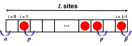
The original TASEP with open-boundary conditions is defined as a one-dimensional lattice (lane) of sites, which are labeled from left to right as , as illustrated in Fig. 1. Each site can be either empty or occupied by only one particle. When the th site at time is occupied by a particle, its state is represented as ; otherwise, its state is .
Discrete time and parallel updating are adopted in the present study. During parallel updating, the states of all the particles on the lattice are determined simultaneously in the next time step. Particles enter the lattice from the left boundary with input probability , and they leave the lattice from the right boundary with output probability . In the bulk, particles whose right-neighboring sites are empty can hop to the rightward site with probability ; otherwise they remain at their present site. The modified TASEP differs from the original process in the following two respects.
II.2 Modification 1: Updating rules
Our modified updating rules have two-step structure. First, particles hop deterministically one site forward regardless of the right-neighboring site, which reproduces an important feature of an escalator.
In addition, particles may hop one more site forward with hopping probability , which is fixed throughout each lattice in our model, if the right-neighboring site is empty. This possibility represents walking on an escalator.
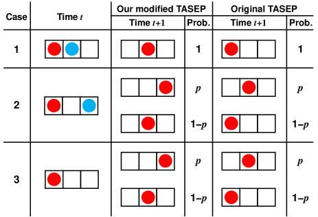
So, particles can hop one or two sites for each time step. We note that in our model particles have two opportunities for hopping and can hop one or two sites in each time step, unlike the Nagel-Schreckenberg model for vehicular traffic Nagel and Schreckenberg (1992), in which particles hop equal to or more than zero site only once in each time step. Table I summarizes the modified updating rules in comparison with the original updating rules.
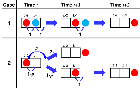
At the right boundary, a particle can leave the system from the ()th site or from the ()th site, unlike in the original TASEP, in which only a particle occupying the ()th site leaves the system with output probability . In the present model, a particle occupying the ()th site at time leaves the system with probability and hops to the ()th site with at time () if ; otherwise it hops to the ()th site. On the other hand, a particle occupying the ()th site at time must leave the system. Table II extracts and summarizes the updating rules around the right boundary.
II.3 Modification 2: Two lanes with two types of particles
Second, our modified model consists of two lanes. The state of the th site of the lane 1 and 2 at time are represented as and , respectively. Each lane can act as a standing lane () or a walking lane (). Changing lanes is prohibited.
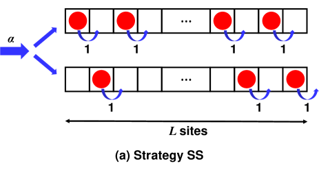
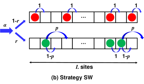
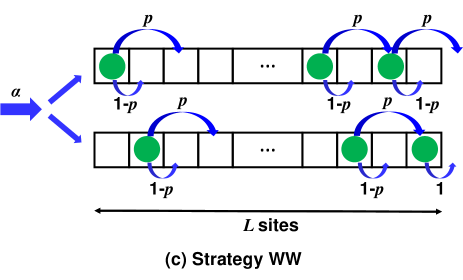
Now, we consider three strategies: (1) two standing lanes, which corresponds to Strategy SS (see Fig. 2 (a)), (2) one standing lane with one walking lane, corresponding to Strategy SW (see Fig. 2 (b)), and (3) two walking lanes, corresponding to Strategy WW (see Fig. 2 (c)). Strategy WW is generally not adopted in real situations; however, it is investigated here for the sake of comparison.
With Strategy SS and WW, particles can enter either of the two lanes if the first site is empty. Specifically, a particle enters lane 1 (lane 2) if (if ), while it must select enter either of two lanes if indiscriminately, i.e., with probability 1/2.
We emphasize that particles can always enter the system with Strategy SS and WW. This is because all the particles in the system will hop one or two sites forward every time step, so at least one of the two left boundaries will always be vacant; that is, , , or .
With Strategy SW, however, two types of particles are possible; waking-preference particles with probability and standing-preference particles with probability . Standing (walking) particles can enter the standing (walking) lane if the leftmost site of the corresponding lane is empty; otherwise they cannot. Unlike Strategy SS and WW, particles frequently cannot enter the system in this case because of the preference. We note that in the simulations below the preference of a particle is determined just before it enters the system; this preference is reset if the particle cannot enter and is redetermined at the next chance of entering.
III One-lane model
with the modified updating rules
In this section, we briefly discuss the steady-state flow of the basic one-lane model with the modified updating rules.
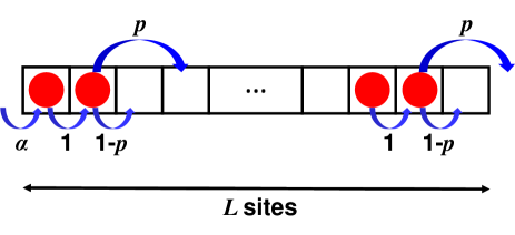
The basic one-lane model with our modified updating rules, as illustrated in Fig. 3. In this system, particles must hop one or two sites forward. Therefore, the steady-state flow is clearly equal to or more than that of the original TASEP with hopping probability .
The original TASEP with for various () exhibits only two phases; the low-density (LD) phase, in which the system is governed by the left boundary, and the high-density (HD) phase, in which the system is governed by the right boundary, and the maximal current (MC) phase, in which the system is governed by the bulk, never occurs. Therefore, the one-lane model is always governed by the left boundary, since a queue can never form near the right boundary. This fact, counter-intuitively, indicates that the flow is determined regardless of , so the flow is always constant. This can be explained as follows.
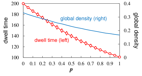
First, walking clearly reduces the dwell time of each particle in the system, which is defined as the time gap between the time when the particle enters the system and the time when it leaves. The dwell time decreases as increases. In addition, the global density of the lane, which is defined as the average number of occupied cells over the space in one time step, decreases as increases, due to the longer gap between particles. Figure 4 shows the average dwell time and the global density as functions of , and reproduce the behavior discussed above. Since (i) the average velocity of particles is proportional to the dwell time, and (ii) the flow is represented as a multiplication of the average velocity and the global density, the flow remains constant.
The steady-state flow of the one-lane model with our updating rules satisfies
| (1) |
resulting in
| (2) |
Eq. (2) is equal to that of the original TASEP in the LD phase with parallel updating, indicating that the one-lane system always exhibits the LD phase.
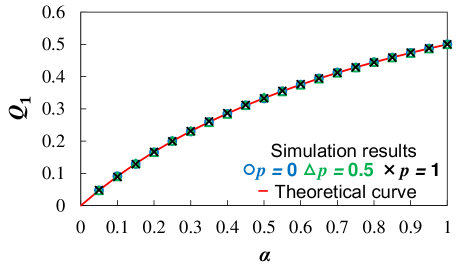
Figure 5 compares the simulation (dots) and theoretical (curve) values of as functions of for various . In the simulations, we set and the flow is obtained by averaging over time steps after evolving the system for time steps (and similarly hereafter).
In Fig. 5, the simulation values show very good agreement with the theoretical curve, and at the same time, the simulations also confirm that is independent on .
IV Total (macro-scale)
transportation time
with the two-lane model
In this section, we investigate the total (macro-scale) transportation time of particles with the two-lane model. Specifically, is defined as the time gap between the start of the simulation and the time at which the final leaving particle leaves the system. The total transportation times with Strategy SS, SW, and WW are represented as , , and , respectively.
IV.1 Steady-state flow , , and
Before examining , we briefly discuss the steady-state flow in the two-lane model.
Since particles can always enter the system with Strategy SS and WW (see Subsec. II.3), the following relation holds
| (3) |
where and are defined as the steady-state flow of the two-lane model with Strategy SS and WW, respectively. We emphasize that counter-intuitively, because of the independence of the flow from (see the previous section), so walking can have no effect on increasing the steady-state flow.
Second, with Strategy SW, particles prefer to enter a standing lane or a walking lane with some probability. Given that a particle prefers standing (walking) with probability (), the input probability of the standing (walking) lane reduces to (). Therefore, the steady-state flows of the standing lane and the walking lane in the two-lane model are given as
Consequently, the steady-state flow of the two-lane model with Strategy SW, , can be calculated as
| (6) |
which takes its maximum value when . The detailed properties of the function of Eq. (6) are discussed in Appendix A.
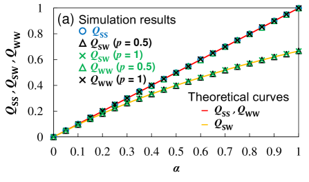
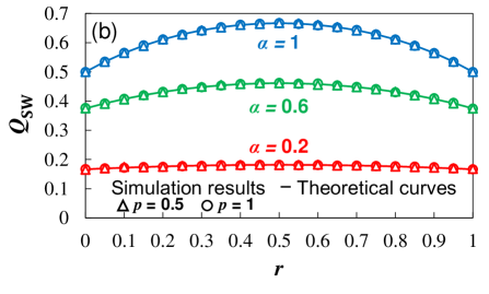
Figure 6 compares the simulation (dots) and theoretical (curves) values of (a) , for , and for as functions of , and (b) for various and as functions of . The simulation values again show very good agreement with the theoretical curves.
From Eqs. (3) and (6), we immediately obtain
| (7) |
indicating that Strategy SS (WW) is always advantageous in terms of steady-state flow.
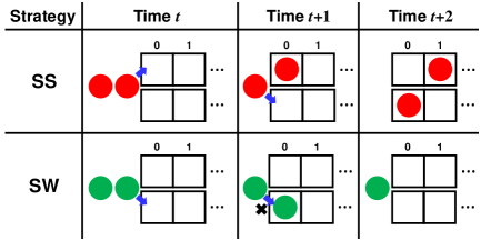
The absolute advantage of Strategy SS (WW) over Strategy SW is explained with the behavior at the entrances of the lanes. Table III summarizes the model behavior at the left boundary, extracting the first and second site with .
With Strategy SS (WW), since consecutive pairs of particles mutually enter either lane, two particles can enter the system in two time steps, as shown in the upper panel of Tab. III.
On the other hand, with Strategy SW they cannot enter the system with two time steps but with three time steps, if both of two consecutive particles’ preference are the same, as shown in the lower panel of Tab. III. The two particles can enter the system in two time steps if two consecutive particles separately prefer walking and standing. Therefore, is maximized if , which clearly maximizes the probability that the preferences of the two consecutive particles differ.
Considering that the system is governed by the left boundary, these facts finally lead to , explaining the absolute advantage of Strategy SS (WW) over Strategy SW.
IV.2 Total (macro-scale) transportation time
IV.2.1 Approximate theoretical analyses of
In this subsection, we theoretically calculate the approximations of (total transportation time with Strategy SS), (total transportation time with Strategy SW), and (total transportation time with Strategy WW) and consider the relations among them.
Considering that the steady-state flow expresses the average number of particles that pass a certain point (the left boundary) each time step, the average required time steps for the th particle to enter the system from the time at which the first-entering particle enters in steady-state flow can be calculated as
| (8) |
On the other hand, the required time steps for the final-leaving particle of both lanes, which is not always identical to the final-entering particle, to reach the right boundary can be represented as
| (11) |
where () is a (an) definitive (approximate) value, and when calculating the possibility that a walking particle is blocked by the particle ahead of it is ignored, resulting in a slight underestimation of (see also Sec. IV.2.2).
Assuming that (i) time steps are needed on average for the first particle to enter the system, and that (ii) particles enter both lanes during the steady-state flow after the first particle enters the system, and — their arguments can be abbreviated unless otherwise specified (similarly for other variables)—can be written as
| (12) |
and
| (13) |
from Eqs. (3), (8), and (11). We note that the first-in-first-out condition—i.e., the entering sequence is identical to the leaving sequence—must be satisfied when Strategy SS is modeled, whereas the relation is mostly satisfied when Strategy WW is modeled.
From Eqs. (12) and (13), and differ only due to the difference in the second term, resulting in if is sufficiently large.
Under the same assumption, we then consider . Unlike and , the first-in-first-out condition generally does not hold since the hopping probabilities of the two lanes are different, leading to difficulty in calculating .
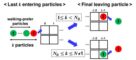
For approximate calculations of , we need to consider the final-entering standing-preference particle and the final-entering walking-preference one. Let us define as a threshold number. Specifically, if a standing-preference particle is (not) included in the last entering particles, the final leaving particle is on average identical to the final-entering standing-preference (walking-preference) particle. We note that if , is always .
Figure 7 gives a schematic illustration of . This figure focuses on the last entering particles, where the th () entering particle from the final-entering particle is identical to the final-entering standing-preference particle. We note that represents that all particles prefer walking, which is defined for the sake of convenience.
Similarly to the assumptions as those applied to and , if we assume that (iii) particles tend to enter the system every time steps, and that (iv) a standing-preference (walking-preference) particle on average stays in the system for () time steps, satisfies
| (12) |
Consequently, reduces to
| (13) |
We note that although is defined to be consecutive, we use its integer part when it is used as the upper limit of summation, which must be an integer.
Regarding as a random variable, i.e., (), can be represented as
| (14) |
where .
Because each particle prefers standing (walking) with probability (), the probability that the th-entering particle from the final one is approximately identical to the final-entering standing-preference particle can be calculated as
| (17) |
satisfying .
Using Eqs. (14) and (17), the expected value of can be calculated as Eq. (LABEL:eq:TSW2). The detailed derivation of is given in Appendix B.
Next, we compare , , and , using Eqs. (12), (13), and (LABEL:eq:TSW2). First, clearly exceeds . In addition, because of Eq. (LABEL:eq:TSW3), also exceeds .
The relation between and is somewhat complicated. Using Eqs. (12) and (LABEL:eq:TSW2), can be calculated as in Eq. (LABEL:eq:TSWTSS).
First, the second part of Eq. (LABEL:eq:TSWTSS) is always equal to or less than 0 (the equal sign holds only when ), and can be regarded as a function of . This is due to the shorter dwell time of walking-preference particles compared to standing-preference particles (see also Fig. 4). We hereafter refer to this effect as the ‘positive effect of walking,’ and it disappears gradually as decreases or increases, since .
On the other hand, the sign of the first part of Eq. (LABEL:eq:TSWTSS) depends on the parameters. For , the first term in the first part is always positive, due to (see Eq. (7)), and can be regarded as a function of .
However, the existence of the second term in the first part of Eq. (LABEL:eq:TSWTSS) invites the result that the first part of Eq. (LABEL:eq:TSWTSS) becomes negative. The numerator of this term satisfies the following relation:
| (19) |
From the definition of , this numerator increases monotonically and converges to a constant value; specifically, when , as increases. From Eq. (13), this constant value can be regarded as a monotonically increasing function of .
Therefore, for sufficiently large , the first part of Eq. (LABEL:eq:TSWTSS) exceeds 0. We hereafter refer this effect as the ‘negative effect of preference,’ because a difference arises due to , which is introduced by the walking/standing preference (see Eq. (7)).
Consequently, for can be rewritten as
| (20) |
where and are, respectively, monotonically increasing functions of and . This fact implies that for sufficiently large the positive effect of walking becomes negligible and (), while this relation can be reversed for small . From Eqs. (12) and (LABEL:eq:TSW2), converges to a certain value as increases, as in Eq. (LABEL:eq:TSW/TSS).
The discussion in this subsection indicates that (i) Strategy WW is always advantageous over Strategy SS and SW, and that (ii) Strategy SS is advantageous over Strategy SW if is sufficiently large; otherwise Strategy SW performs better than Strategy SS.
IV.2.2 Validation of approximations of
This subsection discusses the validity of the theoretical approximations of , , and by comparing them with the results of the numerical simulations.
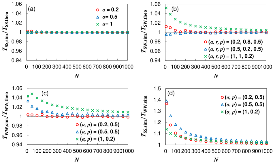
Figure 8 plots the calculated values of the ratios (a) for various , (b) for various , (c) for various , and (d) for various . We average the simulation values of over 1000 trials (and do similarly below for the simulations of unless otherwise specified).
Figure 8 (a) shows that the simulation values of agree with the theoretical ones very well, even for small . Conversely, Figs. 8 (b) and (c) show that the simulation values of and agree with the theoretical ones very well for large ; however, the simulation diverges from the analysis for small and especially if is small. This behavior can be explained as follows.
From Eq. (11), is deterministic, whereas is expected. In addition, although the final-leaving particle is assumed to be able to hop forward freely in the theoretical calculations, it may be blocked by the particle ahead of it in a walking lane, so . These features mean that and can diverge in the theoretical approximations, especially for small and small , as these conditions enhance the influence of on and .
In Fig. 8 (d), is confirmed to approach as increases (strictly speaking, ). From here on, we do not consider , since and , because of the difference in .
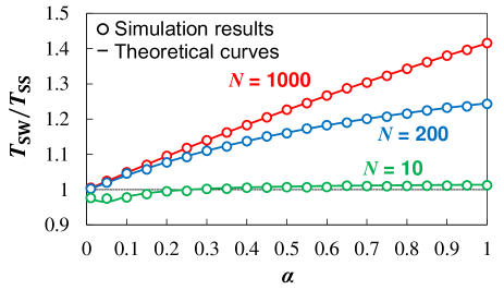
IV.3 Effect of
In this subsection, we investigate the effect of on for various . We set and (in a walking lane).
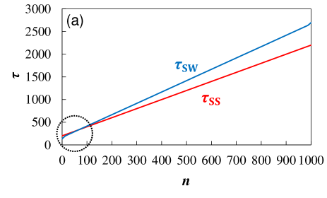
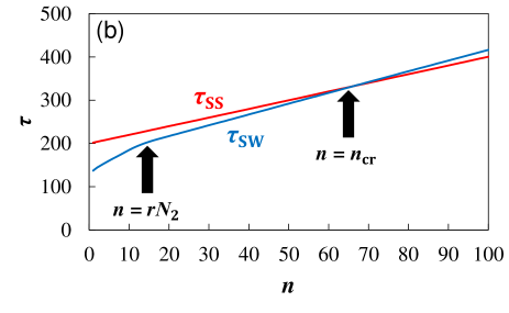
Figure 9 (a) compares and for various as functions of and Fig. 9 (b) is a zoomed-in inset of Fig. 9 (a).
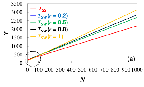
In Fig. 9 (a), we can observe that generally exceeds at least for . This trend means that the negative effect of preference is always greater than the positive effect of walking for large . Moreover, increases as becomes greater. This phenomenon is expected from Eq. (20). We note that the curves for and mostly overlap, even though they are, strictly speaking, different (see also Eq. (LABEL:eq:TSW2))—because the steady-state flows are the same.
On the other hand, in Fig. 9 (b), some cases of appear for small , especially for relatively large . This behavior is because in those limited cases, is influenced very much by the positive effect of walking, i.e., is relatively large.
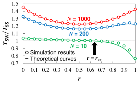
IV.4 Effect of
In this subsection, we investigate the effect of on for various . We set , and (in a walking lane).
Figure 10 compares the simulation (circles) and theoretical (curves) values for the ratio as functions of for various . The simulation results show very good agreement with the theoretical curves. The inequality () means that Strategy SS (Strategy SW) is advantageous.
In Fig. 10, again we see that () regardless of for large ( and 1000 in this figure).
On the other hand, decreases as decreases, and can become less than 1 () for small and small ( and in this figure). This trend is explained as follows.
From Eqs. (3), (6), and (LABEL:eq:TSW/TSS) we obtain
| (22) |
which increases monotonically with respect to . Therefore, for sufficiently large , increases (decreases) as increases (decreases).
Then, taking note of the following two relations:
| (23) |
and
| (24) |
we have Eq. (LABEL:eq:TSWTSSalpha). In Fig. 10, all the plots (curves) are observed to approach 1 as approaches 0. Eq. (23) implies that for small , the negative effect of preference disappears.
Here, we define a new value , where () satisfies
| (26) |
For sufficiently large , always exceeds 0 when , which is discussed in detail in Appendix C.
On the other hand, when , from Eq. (LABEL:eq:TSWTSS),
| (27) |
where is defined as
| (28) |
The behavior of is discussed in detail in Appendix D. We note that for the upper limit of summation when because we need to use the integer part for that case. Eq. (27) indicates that for sufficiently large ; especially,
| (29) |
always exceeds 1, and converges to 1 with , because the negative effect of preference is always greater than the positive effect of walking when .
On the other hand, for small , as decreases, can become below 1, because the positive effect of walking is greater than the negative effect of walking, and finally converges to 1 from Eq. (LABEL:eq:TSWTSSalpha).
IV.5 Effect of
In this subsection, we investigate the effect of on for various . We set and (in a walking lane). We note that only the standing (walking) lane is used and the other lane is always vacant if ().
Figure 11 compares the simulation (circles) and theoretical (curves) values of the ratio as functions of for various . We emphasize that is constant for all values of . The simulation results again show very good agreement with the theoretical curves even though they diverge in very limited cases of small and large ( and in this figure).
This divergence can be explained as follows. First, the positive effect of walking is dominant for small and large , since the influence of the negative effect of preference is small and approaches 1. In addition, although the final leaving particle is assumed to be able to hop forward freely in the theoretical calculations, it can be blocked by the particle ahead of it in a walking lane, leading to a slight underestimation of (see Subsec. IV.2.2). Consequently, small and large enhance the influence of and increase the likelihood of underestimating it when calculating the theoretical values of , so the theoretical curve remains below the simulation values.
In Fig. 11, we see that () for large ( and 1000 in this figure) regardless of , whereas () for small and large ( and in this figure).
In addition, we also note that takes its minimum value near for sufficiently large ( and in this figure), because the negative effect of preference is least active with being slightly more than 0.5, due to the positive effect of walking.
On the other hand, can take a minimum value with for sufficiently small ( in this figure), due to the enhanced positive effect of walking for small and large . Due to the positive effect of walking, even for large .
IV.6 Effect of
In this subsection, we investigate the effect of (in a walking lane) on for various . We set , and . We emphasize that is constant regardless of , as it is when changing .
Figure 12 plots the simulation (circles) and theoretical (curves) values of as functions of for various . The simulation values again show good agreement with the theoretical curves.
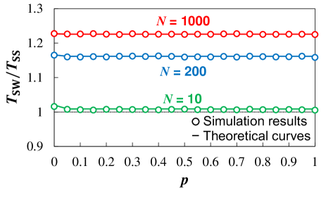
In Fig. 12, we see that () and is hardly affected by , because the steady-state flow does not depend on and the positive effect of walking is very slight when and .
We note that () with , at which both lanes act as standing lanes even when Strategy SW is modeled. In this case, particles can enter either of the two lanes indiscriminately with Strategy SS, while particles still prefer either of the two lanes when Strategy SW is modeled.
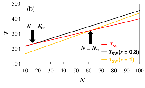
IV.7 Reversal point and

In this subsection, we theoretically determine and , at which (see also Figs. 9—11). These theoretical values are then compared with the simulation values.
From Eqs. (12) and (LABEL:eq:TSW2), for satisfies the following relation:
| (30) |
where .
is generally difficult to obtain for ; however, for the case , the general form of can be obtained easily as
| (31) |
Similarly, () satisfies the following relation:
| (32) |
We note that if no value in that satisfies Eq. (32) exists, indicating that Strategy SS is always advantageous regardless of for a fixed .
Figure 13 compares the simulation (circles) and theoretical (curves) values of (a) as a function of , (b) as a function of , (c) as a function of , and (d) as a function of . When calculating and , the simulation values of were obtained as averages taken over trials. In all figures, the simulations agree well with the theoretical curves.
From the definition of (), (Strategy SW is advantageous), if (); otherwise (Strategy SS is advantageous), for fixed (for fixed ). Therefore, these results indicate that Strategy SS is generally advantageous especially for large ; however, in limited cases Strategy SW can perform better than Strategy SS, mainly for small , large , large , and small .
V Individual (micro-scale)
transportation time
with the two-lane model
Now, we introduce the important novel quantity . The quantity is defined as the time gap between the start of the simulation and the time when the th-leaving particle leaves the system, which we refer to as the individual transportation time. The quantity is assumed to be sufficiently small compared to the total number of particles when considering . The individual transportation times with Strategy SS and SW are represented as and , respectively, as when we were discussing .
The quantity clearly coincides with as the first-in-first-out condition is always satisfied with Strategy SS; however, is generally below since the first-in-first-out condition might not hold with Strategy SW. We note that only for and , for which the first-in-first-out condition must be satisfied, so is set to in the following discussion.
V.1 Approximate theoretical analyses of
In this subsection, we theoretically determine approximate values for , for which .
Unlike we did when approximating , we regard the steady-state flow as the average number of particles that pass the right boundary in each step.
In addition, we assume that (i) time steps are needed on average for the first-entering standing-preference (walking-preference) particle to enter the system 111Strictly speaking, these required time steps for each lane are different; however, they are basically small unless approaches very near 0 or 1. Therefore, we simply assume that they are equal to make the calculations easier., and that (ii) particles leave the system in the steady state after the first-leaving particle leaves the system.
Furthermore, the number of particles is assumed to be sufficiently large. Especially, the number of all walking-preference particles needs to be larger than the average number of walking-preference particles that leave the system until the time at which the first-leaving standing-preference particle leaves the system.
We next define the threshold ; specifically, the th-leaving walking-preference particle leaves the system approximately at the same time when the first-leaving standing-preference particle leaves. Therefore, satisfies
| (33) |
which reduces to
| (34) |
Based on the above assumptions, the system behavior can be in three states; (i) both lanes are not yet in steady state, (ii) only the walking lane is in steady state, and (iii) both lanes are in steady state. Table 4 summarizes the states (flows) of the system and relates them to time steps in terms of the model parameters.
| No. | Time | Stand | Walk | Entire |
|---|---|---|---|---|
| 1 | R.P. (0) | R.P. (0) | R.P. (0) | |
| 2 | R.P. (0) | S.S. | R.P. | |
| 3 | S.S. | S.S. | S.S. |
Consequently, if we note the first particles leave the system with and the next () particles leave with , reduces to
| (35) |
On the other hand, since , can be written as
| (36) |
from Eq. (12).
| (37) |
The quantity is clearly smaller than for , so . Therefore, finally reduces to
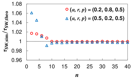
V.2 Comparison with simulation results
In this subsection, we compare the theoretical approximations, obtained in the previous subsection, with simulation results.
First, Fig. 14 shows the values of the ratio as a function of for . The simulation values show very good agreement with the theoretical ones for . We note that the comparison regarding is abbreviated since .
Next, Fig. 15 compares the simulation values of and as functions of , with fixed . In Figs. 15 (a) and (b), we see a point , in which is defined as . This phenomenon can be explained qualitatively as follows.
At first, some of the first entering waking-preference particles leave the system when Strategy SW is simulated more quickly than when Strategy SS is simulated. In this case, for small the positive effect of walking has the dominant effect on , so . After some time has elapsed, the negative effect of preference becomes dominant, resulting in .
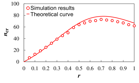
Finally, Fig. 16 compares the simulation (dots) and theoretical (curve) values for as a function of . In Fig. 16, the simulation values show relatively good agreement with the theoretical curves. The upper (lower) bound of the curve of indicates the number of particles that can leave the system more quickly with Strategy SS (Strategy SW) than with Strategy SW (Strategy SS), even if is large.
In addition, takes the maximal value around in Fig. 16. If we notice the third term of in Eq. (35) for , the numerator is maximized when (see also Eq. (34)), while the denominator is maximized when (see Appendix A). The former (latter) corresponds to the positive effect of walking (the negative effect of preference). Therefore, for fixed , takes its maximum value in the range , which implies that also takes its maximal value in the range .
VI CONCLUSION
We have analyzed three strategies for movement on an escalator: (i) two standing lanes (Strategy SS), (ii) one standing lane plus one walking lane (Strategy SW), and (iii) two walking lanes (Strategy WW). These strategies were modeled with a modified two-lane TASEP. The specific contributions of this study are as follows.
In Sec. III, we found that the one-lane model with our modified updating rules exhibits only the LD phase for all values of , and that the steady-state flow for any is identical to that of the original open-boundary TASEP with . This indicates that walking on an escalator does not affect steady-state flow, which is consistent with the results in Yue et al. (2018).
In Sec. IV, we considered the total transportation time using theoretical analysis and numerical simulations. In steady state, is equal to and is always greater than . For example, decreases at — compared to in the most-congested situations (). This finding is consistent with the results of a pilot performed in the London underground in 2015 Kukadia et al. (2016); when ‘standing only’ was specified for escalators at Holborn station, about more customers could use an escalator during the busiest times when both lanes were used only for standing.
Since , counter-intuitively, for sufficiently large , and is generally smaller than , indicating that Strategy SS is advantageous for large . On the other hand, in limited cases for small , Strategy SW can be more useful. Those differences arise because the negative effect of preference generally exceeds the positive effect of walking with Strategy SW for large , while this relation is reversed for small .
We have determined the reversal point and , which satisfies and . These values confirm that Strategy SW is advantageous mainly for small , large , large , and small .
In Sec. V, we considered the individual transportation time using theoretical analysis and numerical simulations. Even if is large, in which Strategy SS is advantageous in terms of reducing , the first-leaving particles, mainly including walking-preference particles, can leave the system more quickly under Strategy SW than under Strategy SS. This behavior arises because the positive effect of walking is more active than the negative effect of preference in this case.
Applying the results of the present paper to real situations, we find that encouraging pedestrians to only stand on an escalator, which has recently been suggested by practitioners, is indeed beneficial for improving pedestrian flow, especially when a large number of pedestrians (large ) are using a facility. Conversely, providing a walking lane can improve pedestrian flow in limited cases in which the entrance is relatively uncongested (small ), the fraction of walking-preference pedestrians is high (large ), and the walking velocity is large (large ) with a small number of pedestrians (small ). In addition, the first-entering walking-preference pedestrians tend to benefit from Strategy SW, even if the number of pedestrians is large (large ).
More realistic models and comparisons with field data will be needed to more clearly relate our findings to the real world. For example, combining multiple models of escalators and floor fields, like a cellular-automaton pedestrian model Burstedde et al. (2001), remains as a future work, along with fitting using actual data. Even so, the simple model discussed above offers useful insights as a first step.
ACKNOWLEDGMENTS
We greatly appreciate Airi Goto for her fruitful comments. This work was partially supported by JST-Mirai Program Grant Number JPMJMI17D4, Japan, JSPS KAKENHI Grant Number JP15K17583, and MEXT as gPost-K Computer Exploratory Challenges h (Exploratory Challenge 2: Construction of Models for Interaction Among Multiple Socioeconomic Phenomena, Model Development and its Applications for Enabling Robust and Optimized Social Transportation Systems) (Project ID: hp180188).
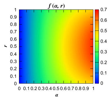
Appendix A Properties of
In this appendix, we briefly give the details of the properties of , i.e., Eq. (6), as a function of and .
Defining as
| (39) |
can be rewritten as
| (40) |
Therefore, for fixed (), is obviously a monotonically increasing function of (). We assume that is constant hereafter.
Replacing with for simplicity, can be written as
| (41) |
where . Taking the first derivation of , is calculated as
| (42) |
The results of the first derivative test are summarized in Tab. 5. takes its maximum value with ().
| 0 | … | … | |||
|---|---|---|---|---|---|
| 0 |
Appendix B Detailed calculation of
In this appendix, we discuss the detailed calculations for obtaining the general form of .
The specific calculations are summarized as Eq. (B1). We note that the third term of the fourth line in Eq. (B1) is the summation of an arithmetico-geometric sequence, and therefore, we can obtain a closed-form expression.
Appendix C Discussion of the behavior of
when for sufficiently large
In this appendix, we briefly discuss the behavior of when for sufficiently large .
For sufficiently large ; especially , , due to . Therefore, using Eq. (LABEL:eq:TSWTSS), can be represented as follows:
| (43) |
where , , and can be regard as constant values; specifically,
| (44) |
| (45) |
and
| (46) |
Noting that the the denominators of the first (second) terms of Eq. (43) clearly increase (decrease) monotonically with respect to , from Eq. (43)—(46) we see that is a monotonically increasing function of .
Considering that for and sufficiently large , always exceeds 0 for .
Appendix D Discussion of the behavior of
when for sufficiently large
Here, we discuss the details of the behavior of when for sufficiently large . The function can be rewritten as follows:
| (47) |
where and are represented as
| (48) |
and
| (49) |
For sufficiently large , which especially satisfies and ; specifically,
| (50) |
can be calculated as
| (51) |
Therefore, for sufficiently large , is a monotonically increasing function when . Considering this fact together with , , and therefore,
| (52) |
when .
References
- Elevator (1971) T. Elevator, American National Standard Safety Code for The American Society of Mechanical Engineers, ANSI A 17 (1971).
- Strakosch (1998) G. R. Strakosch, The vertical transportation handbook (John Wiley & Sons, 1998).
- Mason (2011) M. Mason, Walk the Lines: The London Underground, Overground (Random House, 2011).
- Toda and Takahashi (2018) M. Toda and S. Takahashi, in 2018 IEEE International Conference on Systems, Man, and Cybernetics (SMC) (IEEE, 2018) pp. 1156–1161.
- Toki (nese) M. Toki, Bulletin of Edogawa University 25 (2015, in Japanese).
- bbc (2019) ‘Escalator etiquette: The dos and don’ts’, BBC News (28 July, 2013, accessed February 22, 2019), https://www.bbc.com/news/magazine-23444086.
- age (2019) ‘Keep it to the left’, THE AGE (July 29, 2005, accessed February 22, 2019), https://www.theage.com.au/national/keep-it-to-the-left-20050729-ge0lhc.html.
- Kukadia et al. (2016) C. H. N. Kukadia, P. Stoneman, and G. Dyer, NECTAR , 11 (2016).
-
JR (2019)
’Campaign on Non-walking in
escalators in Tokyo Station (in Japanese)’, JR
East (11 December, 2018, accessed February 22, 2019), https://www.jreast.co.jp/press/
2017/tokyo/20181211_t01.pdf. -
nyt (2019)
‘Why You Shouldn ft Walk on
Escalators’, The New York Times (April 4, 2017, accessed February 22, 2019), https://www.nytimes.com/2017/04/04/us/
escalators-standing-or-walking.html. - Kauffmann (2011) P. Kauffmann, Ph.D. thesis, Virginia Tech. (2011).
- Li et al. (2015) W. Li, J. Gong, P. Yu, S. Shen, R. Li, and Q. Duan, Physica A 420, 28 (2015).
- Al Widyan et al. (2016) F. Al Widyan, A. Al-Ani, N. Kirchner, and M. Zeibots, in Australasian Transport Research Forum (ATRF, 2016).
- Cheung and Lam (1998) C. Cheung and W. H. Lam, J. Traffic Transp. 124, 277 (1998).
- Ji et al. (2013) X. Ji, J. Zhang, and B. Ran, Physica A 392, 5089 (2013).
- Kauffmann and Kikuchi (2013) P. Kauffmann and S. Kikuchi, Transport Res. Rec. , 136 (2013).
- Yue et al. (2018) F.-R. Yue, J. Chen, J. Ma, W.-G. Song, and S.-M. Lo, Chin. Phys. B 27, 124501 (2018).
- Parmeggiani et al. (2003) A. Parmeggiani, T. Franosch, and E. Frey, Phys. Rev. Lett. 90, 086601 (2003).
- Chowdhury et al. (2005) D. Chowdhury, A. Schadschneider, and K. Nishinari, Phys. Life Rev. 2, 318 (2005).
- Chou et al. (2011) T. Chou, K. Mallick, and R. Zia, Rep. Prog. Phys. 74, 116601 (2011).
- Appert-Rolland et al. (2015) C. Appert-Rolland, M. Ebbinghaus, and L. Santen, Phys. Rep. 593, 1 (2015).
- Helbing (2001) D. Helbing, Rev. Mod. Phys. 73, 1067 (2001).
- Imai and Nishinari (2015) T. Imai and K. Nishinari, Phys. Rev. E 91, 062818 (2015).
- Ito and Nishinari (2014) H. Ito and K. Nishinari, Phys. Rev. E 89, 042813 (2014).
- Yamamoto et al. (2017) H. Yamamoto, D. Yanagisawa, and K. Nishinari, J. Stat. Mech. 2017, 043204 (2017).
- Yanagisawa et al. (2010) D. Yanagisawa, A. Tomoeda, R. Jiang, and K. Nishinari, JSIAM Lett. 2, 61 (2010).
- Arita and Yanagisawa (2010) C. Arita and D. Yanagisawa, J. Stat. Phys. 141, 829 (2010).
- Arita and Schadschneider (2015) C. Arita and A. Schadschneider, Math. Mod Meth. 25, 401 (2015).
- de Gier and Nienhuis (1999) J. de Gier and B. Nienhuis, Phys. Rev. E 59, 4899 (1999).
- Blythe and Evans (2007) R. A. Blythe and M. R. Evans, J. Phys. A 40, R333 (2007).
- Derrida et al. (1993) B. Derrida, M. R. Evans, V. Hakim, and V. Pasquier, J. Phys. A 26, 1493 (1993).
- Evans et al. (2011) M. Evans, Y. Kafri, K. Sugden, and J. Tailleur, J. Stat. Mech. 2011, P06009 (2011).
- Wang et al. (2014) Y.-Q. Wang, R. Jiang, Q.-S. Wu, and H.-Y. Wu, Mod. Phys. Lett. B 28, 1450123 (2014).
- Hilhorst and Appert-Rolland (2012) H. Hilhorst and C. Appert-Rolland, J. Stat. Mech. 2012, P06009 (2012).
- Reichenbach et al. (2007) T. Reichenbach, E. Frey, and T. Franosch, New J. Phys. 9, 159 (2007).
- Nagel and Schreckenberg (1992) K. Nagel and M. Schreckenberg, J. de Phys. I 2, 2221 (1992).
- Note (1) Strictly speaking, these required time steps for each lane are different; however, they are basically small unless approaches very near 0 or 1. Therefore, we simply assume that they are equal to make the calculations easier.
- Burstedde et al. (2001) C. Burstedde, K. Klauck, A. Schadschneider, and J. Zittartz, Physica A 295, 507 (2001).