Stokes inversion based on convolutional neural networks

Abstract

Context. Spectropolarimetric inversions are routinely used in the field of solar physics for the extraction of physical information from observations. The application to two-dimensional fields of view often requires the use of supercomputers with parallelized inversion codes. Even in this case, the computing time spent on the process is still very large.

Aims. Our aim is to develop a new inversion code based on the application of convolutional neural networks that can quickly provide a three-dimensional cube of thermodynamical and magnetic properties from the interpreation of two-dimensional maps of Stokes profiles.

Methods. We trained two different architectures of fully convolutional neural networks. To this end, we used the synthetic Stokes profiles obtained from two snapshots of three-dimensional magneto-hydrodynamic numerical simulations of different structures of the solar atmosphere.

Results. We provide an extensive analysis of the new inversion technique, showing that it infers the thermodynamical and magnetic properties with a precision comparable to that of standard inversion techniques. However, it provides several key improvements: our method is around one million times faster, it returns a three-dimensional view of the physical properties of the region of interest in geometrical height, it provides quantities that cannot be obtained otherwise (pressure and Wilson depression) and the inferred properties are decontaminated from the blurring effect of instrumental point spread functions for free. The code, models, and data are all open source and available for free, to allow both evaluation and training.

1 Introduction

Although numerical magneto-hydrodynamic (MHD) simulations of the solar atmosphere (especially in the photosphere) are already in an advanced state (see, e.g., Rempel, 2012; Cheung et al., 2010a, 2018), we continue to rely on the interpretation of spectropolarimetric signals with relatively simple empirical parametric models to determine magnetic fields and thermodynamic properties of different structures in the solar atmosphere. The parametric nature of these empirical models makes it straightforward to tune the model parameters until a good fit is obtained to the signals, so that it is relatively simple to extract the relevant information.

The inference of atmospheric parameters from Stokes profiles is done by proposing a forward model $\mathbf{I}(\boldsymbol{\theta},\lambda)$ that describes the spectral shape of the four synthetic Stokes profiles depending on a set of model parameters $\boldsymbol{\theta}$. In general, fitting the model for the Stokes parameters to the observations is a nonlinear nonconvex inverse problem that is plagued with problems: difficulty in convergence, ambiguities as a consequence of the potential presence of several local minima (also extended minima in the hyperspace of parameters) and computational problems due to the complexity of the forward problem. In recent decades several models of increasing complexity have been proposed. The simplest ones are based on the Milne-Eddington atmosphere, which provides an analytical solution to the radiative transfer equation and results in an simple functional form for the emerging Stokes parameters (Auer et al., 1977; Landi Degl’Innocenti & Landolfi, 2004). More complicated models require the presence of gradients along the line-of-sight (LOS). They were first implemented by Ruiz Cobo & del Toro Iniesta (1992) in the code “Stokes Inversion based on Response functions” (SIR) and it was based on the assumption of local thermodynamical equilibrium (LTE) plus that of hydrostatic equilibrium in the atmosphere. SIR describes the depth stratification of the atmosphere in terms of a few nodes (their position and number are hyperparameters that are typically selected by the user) and the rest of the stratification is obtained by a smooth interpolation. This type of approach has been reimplemented later in many other codes, some of them fundamentally similar like SPINOR (Frutiger et al., 2000), Helix+ (Lagg et al., 2004) or VFISV (Very Fast Inversion of the Stokes Vector; Borrero et al., 2011). Other codes have relaxed some of the initial hypothesis of SIR. Examples include NICOLE (Socas-Navarro et al., 2015) which relaxes the hypothesis of LTE and can extract information from strong chromospheric lines, STiC (de la Cruz Rodríguez et al., 2018) which deals with lines with strong partial redistribution, needed for very strong lines forming in the upper chromosphere or transition region, or Hazel (Asensio Ramos et al., 2008) which deals with lines whose polarization is controlled by scattering polarization, the Hanle and Zeeman effects but in simplified model atmospheres.

In recent years, more than two decades after the publication of the SIR code, we are witnessing a bright new era in the development of inversion codes, with new ideas all around. This is a consequence of several facts: i) the availability of more computing power, ii) the development and application of new techniques and algorithms and iii) the imminent advent of the 4m class telescopes in solar physics with DKIST (Daniel K. Inouye Solar Telescope; Rimmele et al., 2012) and the European Solar Telescope (EST; Collados et al., 2013) which will produce data of unprecedented quality and at an unprecedented rate. From our perspective, one of the first examples of this development was produced by van Noort (2012), who proposed a spatially coupled inversion code in which the point spread function (PSF) of the telescope couples together many pixels in the field-of-view (FOV). The coupling produces that the inversion problem becomes global in the FOV and the model atmosphere for all pixels have to be simultaneously inferred. The solution of the optimization problem via a Levenberg-Marquardt (LM) algorithm required the calculation of a Hessian matrix that couples all pixels. Because the PSF is spatially compact, the Hessian matrix has some sparsity structure and van Noort (2012) succeeded in exploting this property to invert it, as required by the LM algorithm. However, the depth stratification of the physical quantities is parameterized by a limited number of nodes to make the problem tractable. With this approach, the results are decontaminated from the blurring effect of the PSF of the telescope, thus avoiding the use of ad-hoc stray light contaminations, that often complicates the interpretation of the results. A simpler and, in our personal view, also more controllable approach was proposed by Ruiz Cobo & Asensio Ramos (2013) (see also Quintero Noda et al., 2015) in which deconvolution and inversion is separated in two processes. First the spectropolarimetric data is deconvolved from the telescope PSF using a regularization based on the application of principal component analysis (PCA) to the Stokes profiles. Then the inversion proceeds pixel by pixel as in the usual case. This approach leads to a much simpler and computationally efficient workflow.

Another step forward was the application of the compressed sensing theory (Candès et al., 2006) to spatially regularize the maps of inverted physical properties (Asensio Ramos & de la Cruz Rodríguez, 2015). This approach takes advantage of the presence of spatial correlation in the maps and effectively reduces the number of unknowns that must be inferred. The code developed by Asensio Ramos & de la Cruz Rodríguez (2015) uses a first-order proximal projection algorithm for the optimization of the sparsity-regularized problem. On the downside, precisely the use of first-order optimization techniques produces slow convergence.

Arguably the latest breakthrough in the field of inversion codes has been MASI (MHD-Assisted Stokes Inversion; Riethmüller et al., 2017). This code uses a snapshot of an MHD simulation as a lookup table when carrying out inversions. It works by comparing the observed Stokes parameters in every pixel of the FOV with those of a properly degraded snapshot of an MHD simulation. The 3D cube of physical properties associated with the observations is recovered by stacking the columns of the simulation that better fits the observed Stokes profiles. This 3D cube is obviously not in equilibrium so that it is used as an initial condition in an MHD simulation code until a new equilibrium is found. The procedure is then iterated until an eventual convergence. The resulting inversion code, a result of the combination of a 3D MHD simulation module and a Stokes synthesis module, is computationally demanding. Riethmüller et al. (2017) could only iterate the process twice, though showing clear hints of convergence. In the eventual convergence, one would find a 3D model of the region of interest that also fulfills the MHD equations.

Motivated by the recent enormous success of deep neural networks (DNN; Goodfellow et al., 2016), we propose in this work to leverage DNN to carry out three-dimensional inversions of the solar atmosphere under the assumption of LTE for Hinode-like observations. Our approach is termed SICON (standing for Stokes inversion based on convolutional neural networks). We defer for the future the study of a neural approach for the inversion of spectropolarimetric data at the diffraction limit of a 4m class telescope like DKIST or EST and/or including non-LTE effects. Data-driven approaches using DNNs have already been applied to solar physics, demonstrating striking capabilities to solve problems that could not be solved otherwise or with a much improved precision and/or speed. For instance, we managed to infer transverse velocities from pairs of consecutive images (DeepVel; Asensio Ramos et al., 2017), which allowed us to identify small-scale vortices in the solar atmosphere that last for a few minutes and with sizes on the order of a few hundred kilometers, something impossible with methods based on local correlation tracking (November & Simon, 1988). We have also applied them to compensate for the blurring effect of the telescope and the Earth atmosphere (Díaz Baso & Asensio Ramos, 2018; Asensio Ramos et al., 2018). Illarionov & Tlatov (2018) applied DNNs for the automatic segmentation of coronal holes with great success. The advances in the field of deep learning suggests it is timely to investigate what are the prospects of neural networks in the field of spectropolarimetric inversions. In this paper we leverage convolutional neural networks (CNN; LeCun & Bengio, 1998) that can easily exploit spatial information and the ability to train really deep neural networks that can approximate very nonlinear mappings.

Finally, we point out that the application of neural networks (multi-layer perceptrons; MLP) for the inversion of Stokes profiles is not new. Carroll & Staude (2001) already proposed their use for simple Milne-Eddington inversions and concluded that they were able to obtain physical parameters without any optimization once the neural networks were trained. As additional advantages, they showed their speed, noise tolerance and stability. This was later verified by other works (Socas-Navarro, 2003, 2005). Carroll & Kopf (2008) later expanded their original work to use MLPs to infer the depth stratification in a geometrical height scale of the temperature, velocity and magnetic field vector, as their network was trained with a quiet Sun simulation (Vögler et al., 2005). The application of the neural network pixel by pixel allowed them to recover a tomographic view of the FOV by recombining all individual line-of-sight stratifications. More recently, Osborne et al. (2019) has shown how invertible neural networks (INNs; Ardizzone et al., 2018) can be successfully applied to capture degeneracies and ambiguities in the inference of thermodynamic parameters of plane-parallel chromospheres of flaring regions.

Given the enormous flexibility in the architecture of DNNs, we follow in this paper a double-blind strategy. Both authors, starting from the same training dataset that is described in the following, studied different architectures independently and ended up with two proposals. The general advantages and disadvantages of both architectures (obviously many other architectures are possible) are compared. Both neural networks, with their corresponding trained weights used in this work, can be downloaded from our repository. We anticipate that both architectures give very similar results.

Figure 1: Synthetic continuum images of the snapshots used for training. The left panel shows the sunspot simulation of Rempel (2012) and the right panel shows the emerging flux region simulation of Cheung et al. (2010b).

2 Training sets

Current DNNs are frequently limited only by the properties and quality of the training set (apart from the availability of specialized hardware and time). For our purpose, two possibilities for training could be explored. The first one, that we defer for a subsequent work, is to use standard inversions carried out with codes like SIR. The 2D maps of inferred quantities are then used as training for a deep convolutional neural network. One of the advantages of this approach is that solar physicists are already familiar with these empirical inversions. On the contrary, since the training is done in pixel-by-pixel inversions, the use of CNNs during training only helps in denoising inversions but does not exploit any spatial correlation present in the training data. The second option, which is pursued here, is to use Stokes spectra synthesized in 3D MHD simulations of the solar atmosphere. These simulations might still suffer from a lack of realism but they will eventually become very precise. The advantages of training in these simulations are: i) the CNNs will be able to exploit all the spatial information that is encoded in the training set, ii) deconvolution can be easily implemented during training, iii) information that cannot be obtained using standard inversions can be recovered (like the Wilson depression or the gas pressure). The disadvantage of using simulations as training data is that results might be inaccurate. We expect the results to improve as more advanced simulations are developed. In this sense, our results might be considered as a baseline that are hopefully improved in the near future.

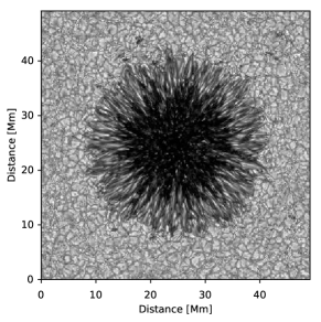
For our purpose we used two different snapshots carried out with the MURaM code (Vögler et al., 2005). The aim of this selection is to provide the neural network with examples of structures that can be found later in real observation so that the properties can be inferred with sufficient generalization. The first one is a snapshot of the sunspot simulation carried out by Rempel (2012). A continuum image at 630 nm is shown in the left panel of Fig. 1. This snapshot shows a well-developed sunspot, with a penumbra of sufficient realism so as to generate the typical penumbral filaments. The snapshot cube is of size 1536$\times$1536$\times$128 with 32 km horizontal (0.044″per pixel) and 16 km vertical grid spacing. This simulation is considered to be the state of the art in the generation of a numerical solar sunspot and its fine structure (Tiwari et al., 2013). One of the problems of this simulation for our purpose is that the sunspot is unipolar, so that a large percentage of the FOV contains only one polarity. For this reason, we artificially generate another snapshot where the magnetic field vector is reversed at each individual grid point. This is a valid procedure under the assumption that this change does not strongly affect the thermodynamics. We expect this to be the case given that the photosphere is a region where the plasma-$\beta$ is large, so the magnetic pressure is negligible in comparison to the gas pressure. We expect in the future to improve our training set by adding another snapshot of a well-developed sunspot simulation with the opposite polarity.

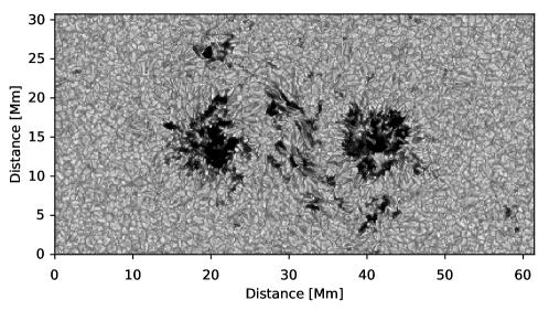
The second snapshot is from the simulation of the formation of an active region on the solar surface by Cheung et al. (2010b). The right panel of Fig. 1 displays the image in the continuum at 630 nm. The snapshot provides a region of large complexity, with opposite polarities in the interface between the two polarities of the active region. The snapshot is of size 1920$\times$960$\times$256 with 48 km (0.066″per pixel) horizontal and 32 km vertical grid spacing.

The synthetic Stokes profiles used during training are obtained after the following process:

1. The synthesis module of SIR is used to compute the Stokes parameters for all the pixels in the two snapshots on the pair of Fe i lines at 6301.5 Å and 6302.5 Å at disk center. SIR requires the the logarithm of the optical depth at 500 nm ($\log\tau_{500}$) as input. For consistency, we compute this axis using the background opacity package inside SIR and discard all depths for which $\log\tau_{500}>2$ because they do not affect the emergent profiles. More precise background opacity packages could have been used but we have verified that a mismatch between the opacity package for the generation of the optical depth axis and that of the synthesis might affect the emergent Stokes profiles significantly, with differences that can be as high as 15-20%. For this reason, we prefer to use SIR as a reference to allow for better comparison with previous results and standard SIR inversions.

2. The synthetic observations are spatially degraded with the Hinode PSF as computed by (Danilovic et al., 2010). The results are rebinned to the Hinode pixel size of 0.16″.

3. The spectra at each spatial point is convolved with the spectral PSF of Hinode and reinterpolated on the standard Hinode wavelength axis of 112 wavelength points. This makes a total of 448 wavelength points for each pixel when all Stokes parameters are serialized. Additionally, the Stokes parameters are normalized to the median continuum in the surrounding quiet Sun.

4. Stokes $Q$, $U$ and $V$ can span several orders of magnitude, typically in the range between 0.1 and 10^-3 (limited by the noise in Hinode). For this reason, we apply a normalization so that the input to the neural networks are around unity. We follow a different strategy in each architecture so that we explain them in detail in the next section.

5. To mimic real Hinode observations, Gaussian noise with a standard deviation of $10^{-3}I_{c}$, with $I_{c}$ the continuum intensity, is added to all Stokes profiles during training.

The physical conditions that will be used during training are treated with the following process:

1. The physical conditions are the temperature, $T$, the vertical velocity, $v_{z}$, the logarithmic gas pressure, $\log P$, and the three cartesian components of the magnetic field, $\mathbf{B}$. They are obtained from the simulation cubes at seven corrugated surfaces of constant optical depth at 500 nm: $\log\tau=0$, $-0.5$, $-1$, $-1.5$, $-2$, $-2.5$ and $-3$. Additionally, the geometric height associated to each one of these surfaces (the Wilson depression for each pixel and optical depth value) is stored. We subtract the average height of the $\log\tau=0$ surface on the quietest region of the snapshot. This makes a total of 49 two-dimensional maps. These maps are rebinned to the Hinode resolution but not degraded with any PSF. In fact, this is somehow problematic because it is well-known that the average Stokes profiles emerging from a set of atmospheres is not equal to the synthetic Stokes profiles in the average atmosphere (e.g., Uitenbroek & Criscuoli, 2011). However, the impact in our case is not too severe because we only need to average 2.4$\times$2.4 pixels for Cheung’s simulation and 3.6$\times$3.6 pixels in the case of Rempel’s snapshot. Other options, that we defer for a future analysis, imply applying superresolution in the DNNs that we consider in Sect. 3 and reduce the effect of the rebinning, eventually going up to the original resolution of the simulation.

2. One of the main issues for inferring the magnetic field is the presence of ambiguous solutions. In the Zeeman regime (the one that we assume for the synthesis of the Stokes profiles) we only find the 180^∘ ambiguity in the azimuth on the LOS. Since we assume observations at disk center, this means that a magnetic field with an azimuth $\phi$ and another one with an azimuth $\phi+\pi$ gives exactly the same Stokes parameters. If this ambiguity is left in the training set, the neural network cannot choose the right solution, so it is mandatory to remove it for a stable training. We do this by using the following three quantities as output instead of the three cartesian components of the magnetic field $(B_{x},B_{y},B_{z})$:

   $$B_{Q} =\mathrm{sign}(B_{x}^{2}-B_{y}^{2}){|B_{x}^{2}-B_{y}^{2}|}^{1/2}$$

   $$B_{U} =\mathrm{sign}(B_{x}B_{y}){|B_{x}B_{y}|}^{1/2}$$

   $$B_{V} =B_{z}.$$ (1)

   The motivation for the labels of the variables is that, in the case of constant magnetic field along the LOS, Stokes $Q$, $U$ and $V$ are proportional to $B_{Q}$, $B_{U}$ and $B_{V}$, respectively. Their advantage is that they are not affected by the 180^∘ ambiguity. The cartesian components of the magnetic field can be obtained by carefully inverting the previous equations and selecting only one of the two compatible solutions.

After all degradations and rebinning, the emerging flux simulation turns out to be of size 397$\times$794 pixels, while the sunspot simulation ends up being of size 424$\times$424 pixels. From these two simulations we randomly extract 50,000 patches of 32$\times$32 pixels with equal spatial probability for training and an extra dataset of 2,000 for validation. The difference in area occupied by the quiet Sun, umbra and penumbra in the two snapshots is not large, so we find unimportant to spatially bias the probability to equally cover the three types of regions. Given that we only have two snapshots, we heavily rely on augmenting the training set by randomly flipping the patches horizontally and vertically and also by rotations of the patches by 90, 180 and 270^∘.

The training of the neural networks is done by optimizing the following scalar loss function, where the summation is carried out over all pixels of all patches in the training set:

$$L=\sum_{i}\left\lVert\mathbf{T}_{i}-\mathbf{f}(\mathbf{W};\mathbf{S}_{i})\right\rVert^{2}.$$ (2)

The loss function measures the $\ell_{2}$ distance between the $i$-th target patch with the physical conditions, $\mathbf{T}_{i}$, and the output of the neural network with weights $\mathbf{W}$ and input Stokes parameter for the very same $i$-th patch, $\mathbf{f}(\mathbf{W};\mathbf{S}_{i})$. Architecture-dependent details of the training are explained later.

3 Architectures

We describe in the following the two architectures that we have used, pointing out their main computational advantages and disadvantages. Contrary to previous studies (Carroll & Staude, 2001; Carroll & Kopf, 2008) in which 1D neural networks were trained, we have used CNNs to exploit the 2D spatial coherence of the FOV. This strategy strongly decreases the model degeneracy due to local noise or multiple minima and also allows us to invert the whole map in one single application of the neural networks.

Figure 2: Encoder-decoder (upper panel) and concatenate architectures (lower panel).

3.1 Encoder-decoder

The first architecture, displayed in the upper panel of Fig. 2 follows the fully convolutional encoder-decoder paradigm, in which the input data is first analyzed by an encoder neural network that acts as a funnel by reducing the spatial dimensionality of the images while increasing the number of channels. This induces the neural network to extract relevant spatial information and encode it in the channel dimension. After the encoding phase, a decoder neural network recovers the original size of the input images. In this case, the only restriction is that, if one wants to get an output of the same dimension as the input, then the input size has to be an integer multiple of $2^{3}$. If this is not the case, the output will have a slightly different number of pixel than the input.

We previously used this architecture in Asensio Ramos et al. (2018) with fantastic performance. Both the encoder and the decoder are based on the concept of residual networks (He et al., 2015), in which skip connections directly connect some layers with later layers. Recent analysis suggest that this not only accelerates training, but also very efficiently removes local minima from the loss hypersurface (Du et al., 2018). We utilize skip connections inside each set of blocks (shown as arrows in the lower part of the blocks) and also between blocks of the same spatial size (shown as arrows in the upper part of the blocks). Additionally, we use the fact that some output parameters have some resemblance with continuum images. This is the case for the temperature and Wilson depression. For these outputs, we simply add the continuum image (in normalized units) directly to the output of the decoder.

The specificities of the encoder-decoder architecture are as follows. To normalize the polarization and prevent it from being ignored by being much smaller than Stokes $I$, we compute the map of maximum amplitude in absolute value (thresholded from below at 5$\times$10^-3) for each Stokes parameter $Q$, $U$ and $V$ and normalize them to each value. The maps of maximum amplitude are then added as input in log scale after subtracting the mean value. Therefore, the total number of input channels is 448+3=451. For that reason, the red blocks in Fig. 2, which refer to input layers are, in this case, patches of size 32$\times$32 with 451 channels. Concerning the output, all physical conditions are linearly transformed to the interval $[0,1]$ using the minimum and maximum values from all available snapshots. When the neural network is used in evaluation, this transformation is undone to recover all physical quantities in the correct units. Finally, we point out that we add a noise realization to the maps of the snapshots used for training and leave it unchanged during the training.

In the encoder-decoder architecture, gray blocks refer to convolutional blocks. They are made of the consecutive application of a batch normalization layer (Ioffe & Szegedy, 2015), a rectified linear unit activation function (ReLU; Nair & Hinton, 2010) and a convolution with a kernel of size 3$\times$3 with a reflection padding of one pixel in the borders to maintain the size of the images. Pink blocks are similar to the gray ones but the convolution is done with a 1$\times$1 kernel. Blue colors are similar convolutional blocks but the convolution is done with a stride of 2, thus reducing the size of the input image by a factor 2, but increasing the number of channels by another factor 2. Orange blocks are made of the consecutive application of batch normalization, ReLU, a bilinear upsampling of a factor 2 and a 3$\times$3 convolution with reflection padding while reducing the number of channels. Finally, the golden layer is the output, in our case patches of size 32$\times$32 with 49 channels. The number of channels of each set of blocks is indicated in the figure.

We note that the specific number of blocks and their properties have been set according to previous experience and also encouraged by the successful results showed in the next sections. Although not proven here, we assume that a careful ablation study can produce simpler and faster architectures. Specifically, our election of 32 channels in the first convolutional block is motivated by the expected dimensionality of spectropolarimetric data in the pair of Fe i lines at 630 nm (Asensio Ramos et al., 2007b) and the fact that even a simple linear principal component analysis of the Stokes parameters is able to reconstruct the profiles close to the noise level with only a few eigenprofiles.

Figure 3: Gaussian kernel density estimate of the difference between the physical parameters at different constant optical depth surfaces and the value inferred by the encoder-decoder DNN in the validation set. Results are similar for both architectures.

One of the advantages of the encoder-decoder architecture is that spatial information is efficiently shared. After the three stages of encoding that we use, an image that is originally of size 32$\times$32 turns out to be of size 4$\times$4. A convolution with a kernel of size 3$\times$3 thus couples all pixels in the image at this fourth stage. The output of the network can therefore make efficient use of spatial information from distant structures in the Stokes parameters. This is probably not crucial in our case because Stokes parameters in LTE fundamentally depend on very local information (not much larger than the size of the PSF). However, it introduces an extra robustness that can be very interesting for very extended structures like large sunspots. From a computational perspective, encoder-decoder architectures are memory- and computation-efficient. Images become smaller during the encoder phase, so that convolutions can be made faster and with a lower memory footprint. On the disadvantage side, encoder-decoder networks are sometimes slightly difficult to train.

The scalar loss of Eq. (2) is optimized with respect to $\mathbf{W}$ via the well-known Adam optimizer (Kingma & Ba, 2014). The network has $\sim$3.31 million free parameters. The neural network was trained during 50 epochs with a batch size of 128. The learning rate is 3$\times$10^-4 but it is reduced by a factor of $1/2$ every 30 epochs. The neural network is implemented and trained in PyTorch, which seamlessly allows us to leverage Graphical Processing Units (GPU) to accelerate the calculations (Harker & Mighell, 2012). We used a Titan X and a P100 NVIDIA GPUs for training during the exploration of hyperparameters.

3.2 Concatenate

The second architecture, displayed in the lower panel of Fig. 2, is also fully convolutional. The main difference with the encoder-decoder architecture is that the spatial size of the images is kept fixed throughout the entire architecture. For this second architecture we have opted for a more conservative strategy, similar in philosophy to Carroll & Staude (2001) and Carroll & Kopf (2008), who trained a different network for each physical parameter. The main difference is that the output of mini-networks are concatenated at the end of the topology and we include more physical parameters than previous studies.

One of the advantages of this architecture is that the size in pixels of the input can be arbitrary and does not need to be multiple of any number. While in the encoder-decoder network the spatial dimensionality of the input is reduced thanks to the bottleneck, a similar compression effect can be achieved in this case by reducing the flexibility of the connectivity or reducing the number of kernels of each convolutional layer in the network. On the downside, by having a mini-network for each physical variable, this architecture does not exploit the common patterns and relationships among the different physical parameters. Consequently, it needs a large number of network parameters to achieve high accuracy. Despite these differences, many of the details discussed in the previous section about accelerating the training and improving the accuracy still applies to this case.

The specificities of the concatenate architecture are as follows. As before, the red block in the lower panel of Fig. 2 refers to input layers, in our case patches of size 32$\times$32 with 448 channels, that is, just four Stokes parameters with 112 wavelength points each. The normalization in this case is very simple (1 for Stokes $I$ and 0.1 for Stokes $Q$, $U$ and $V$). The accuracy of the network is good using this simple scaling, which makes all Stokes parameters have roughly the same order of magnitude. Finally, noise is added online during the creation of each batch, so it changes from epoch to epoch.

Gray blocks in the lower panel of Fig. 2 refer to convolutional blocks, which are slightly different to those of the encoder-decoder case. They are built by the consecutive application of a convolution with a kernel of size 3$\times$3 with a reflection padding and an exponential linear unit activation function (ELU; Clevert et al., 2015). This activation function has been proven to speed up learning while leading to higher accuracies than using batch normalization layer followed by a ReLU activation function, like in the encoder-decoder architecture. ELUs allow negative values to pass through the network, thus forcing the mean response of the neurons to lie closer to zero but with a clear saturation plateau in its negative regime. This allows networks to learn more robust and stable representations. Additionally, the loss function presents a smoother decrease during convergence as compared with using ReLUs.

Figure 4: Synthetic continuum image of the validation snapshot from the emerging flux region simulation of Cheung et al. (2010b).

While the first two gray blocks have 32 channels each, the last gray blocks has 7 channels to match the number of depths used for each parameter. The last dark gray block is the only block that performs convolutions without activation. The result of each dark gray block is then concatenated at the end for producing the output without any additional transformation (indicated with dashed arrows above the network). Similarly to the previous case, each physical parameter is transformed to be close to unity when possible by using the following units: the temperature in kK, the velocity in km s^-1, the magnetic field components in kG, and the geometrical height in Mm. Since the spatial size of the images is kept in each convolutional layer, we do not utilize any pooling or upsampling operation. Each output of the concatenate architecture is the result of 4 convolutional blocks with $3\times 3$ kernels. Although the first block produces a receptive field of size $3\times 3$ for each neuron, the second block increases that to $5\times 5$, the third one to $7\times 7$ and the last one to $9\times 9$. Such a receptive field is able to couple, for a single pixel in the output, the Stokes parameters of a patch of $\sim 1.44^{\prime\prime}$, which is almost 5 times the diffraction limit of Hinode/SOT. This size is very similar to the size of the PSF considered in the coupled inversions carried out by van Noort (2012).

The total number of free parameters in this architecture is $\sim 1$ M free parameters. We train the network using Adam with a constant learning rate of $10^{-4}$ during 20 epochs with a batch size of 10. This neural network was implemented and trained in Keras, which also allows us to leverage GPUs to accelerate the calculations.

Figure 5: Gaussian kernel density estimate of the difference between the physical parameters at different constant optical depth surfaces and the value inferred with SIR.

4 Results

Once the DNN is trained, it can be applied to any Hinode observation, provided that the data is preprocessed in the same way. This preprocessing requires simply to normalize to the local average quiet Sun and carry out the specific normalizion for Stokes $Q$, $U$ and $V$. Given the fully convolutional character of the trained networks, they can be applied to any input, irrespectively of their dimension (taking into account the caveats of the encoder-decoder network). One of the huge advantages of neural networks is their enormous speed during inference. As an example, in a low-profile GPU like the NVIDIA Quadro M4000, the inference of a Hinode map of 512$\times$512 pixels can be done in $\sim$180 ms, which turns out negligible if compared with the time spent in any input/output operation. This speed can be much higher if several maps are used as input as part of a batch, which then would take better advantage of the parallel computation of GPUs. Obviously, using a more modern GPU can cut these times by another appreciable factor. As a consequence, assuming zero overhead in input/output operations, one can carry out 480,000 inversions of 512$\times$512 maps per day with this neural network. The current Hinode database for SOT/SP contains of the order of 12$\times$10³ groups of observations. Assuming that all these groups refer to maps of the quoted size (which is a very conservative upper limit), one can carry out the inversion of the whole Hinode SOT/SP with our proposed neural network in $\sim$36 minutes.

Figure 6: Predicted physical properties of AR10933 using the encoder-decoder network.

Figure 7: Predicted physical properties of AR10933 using the concatenate network.

Figure 8: Total gas pressure at four different optical depth surfaces in the encoder-decoder network. The pressure is measured in cgs units (dyn cm^-2).

Figure 9: Continuum images (left) and zoom of the penumbra region (right). Both architectures provide almost identical results. The first row shows the original Hinode observations. The second row shows the synthetic continuum image in the SIR inversions. The third row refers to the data after the PCA deconvolution process. The fourth row is the synthesis in the model inferred by the neural network. The last row shows the effect of convolving with the Hinode PSF.

4.1 Expected uncertainties

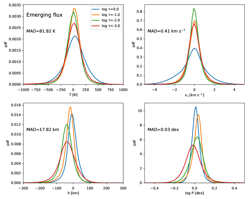
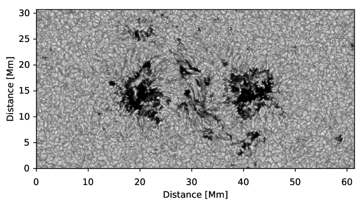
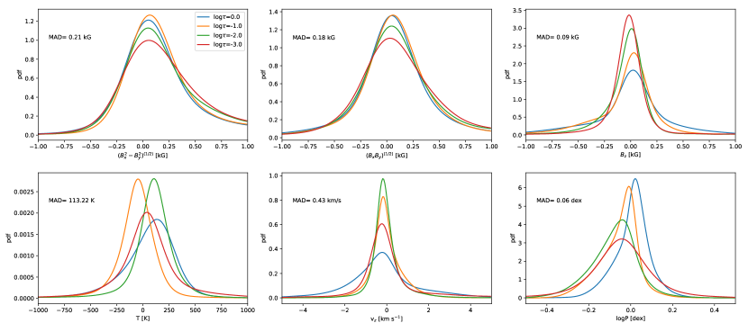
We infer the expected uncertainties by applying the trained neural networks to a different snapshot of the emerging flux simulation of Cheung et al. (2010b), whose continuum image is displayed in Fig. 4. The training and validation snapshots of Cheung et al. (2010b) are separated by 40 minutes in solar time, which is more than enough to produce sufficiently different structures. Given the fully convolutional character of both architectures, we can infer the physical properties on the whole field-of-view in one single run. We compare the output of the neural network with the real value of the physical conditions extracted from the simulation. Figure 3 shows the kernel density estimate of this difference in the encoder-decoder architecture for different optical depth surfaces. For comparison, we also show in Fig. 5 the kernel density estimate of the difference between the physical parameters of the simulation and those inferred by a standard SIR inversion of the synthetic Stokes parameters. The closer to zero, the better our prediction is. The median absolute deviation (MAD; a robust estimation of the standard deviation) is also quoted on each panel. We only quote that associated with $\log\tau=-1$ as representative. However, a detailed analysis of the width of the distributions of Fig. 3 reveals a weak dependence with the sensitivity of the pair of Fe i lines, with slightly broader distributions in higher layers. The resulting uncertainties are very small, in many cases smaller than what one gets from SIR and similar to those obtained by (Carroll & Kopf, 2008). Additionally, we point out that the same results are found for both neural networks. For its novelty, we point out that we are able to find the height of each optical depth surface with an uncertainty below 20 km, which is relevant if compared with that of other approaches (Puschmann et al., 2010; Löptien et al., 2018). Magnetic field components are recovered with uncertainties around 100 G in absolute units. Finally, gas pressures are recovered with uncertainties of $\sim$0.03 dex in cgs units.

Figure 10: Some predicted properties for the complex active region AR11429 and the quiet Sun with the encoder-decoder architecture.

4.2 A simple sunspot

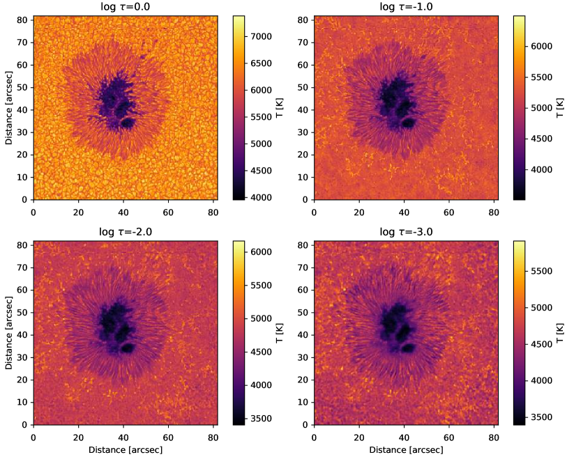
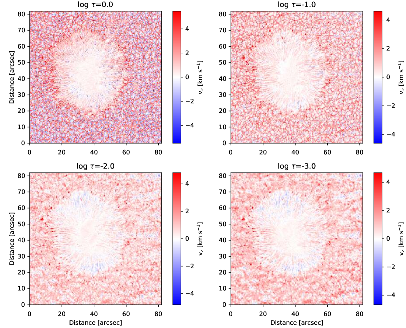
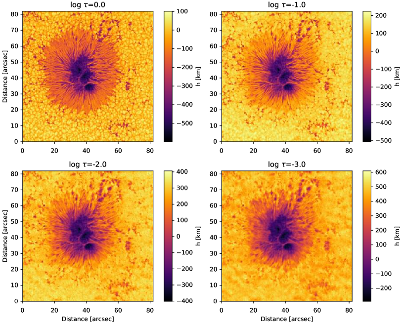
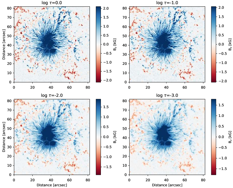
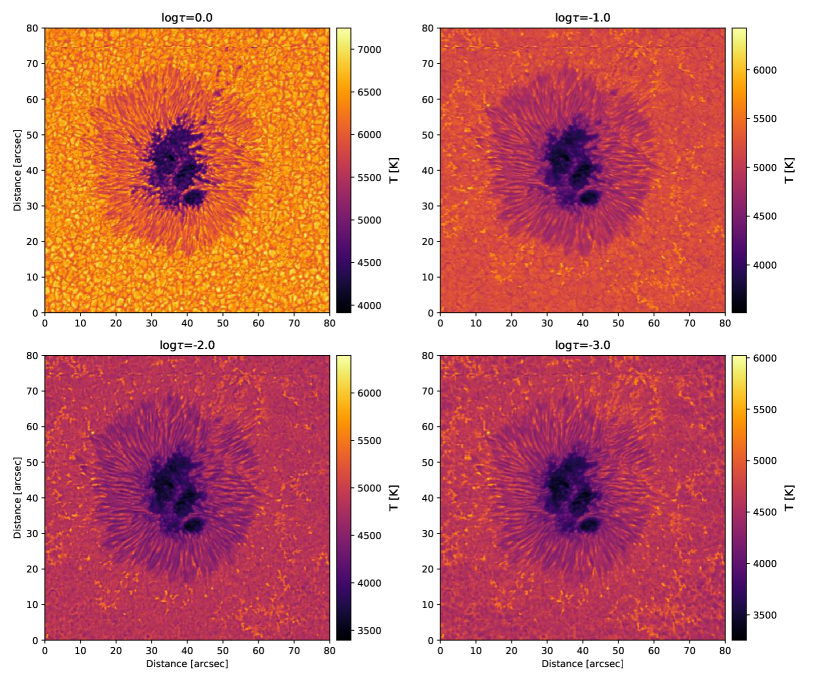
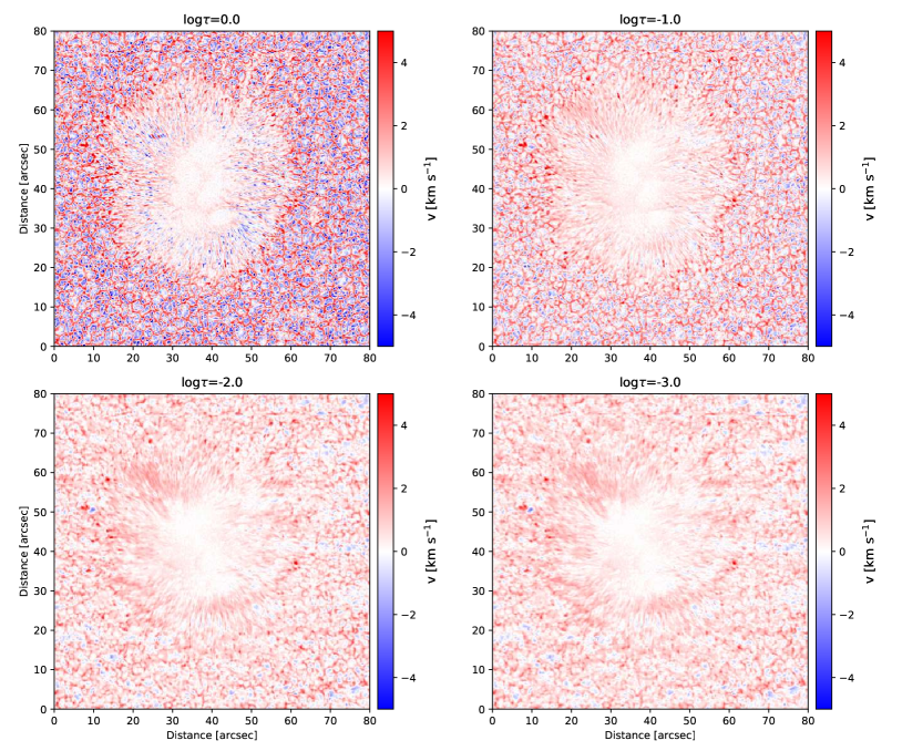
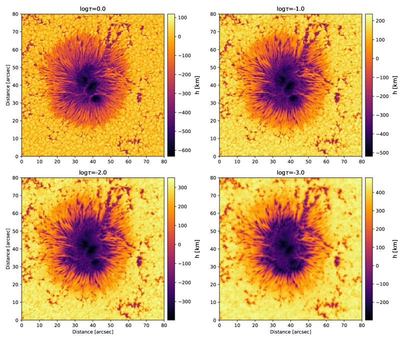
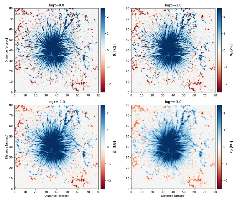
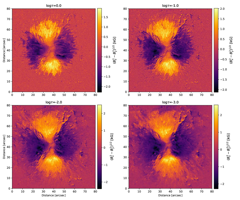
We focus first on a simple sunspot, similar to that used for training. We select the AR10933, observed with Hinode SOT/SP on 2007 January 5 from 11:20 to 14:13 UT. The sunspot is located at coordinates $(-217$″$,-13$″$)$, which gives an heliocentric angle of $\mu=\cos\theta=0.97$. The output of the neural networks at four different optical depth heights are displayed in Fig. 6 for the encoder-decoder architecture and in Fig. 7 for the concatenate architecture. The temperature shows normal granulation at $\log\tau=0$, becoming more diffuse at the height where $\log\tau=-1$. This also happens in the simulation, probably a consequence of the strong faculae around the sunspot. As a consequence, the inverted granulation that we obtain with the neural network approach is not much contrasted. Apart from that, bright structures (brighter than the surrounding quiet Sun) associated with the faculae around the sunspot are seen at high layers. In general, the structure seen in the umbra as umbral dots or light bridges lose contrast in higher layers. Concerning the LOS velocity, we find the umbra practically at rest and the granulation pattern clearly appears for heights above $\log\tau=0$.

Of special interest is the inference of the height of each pixel. We obtain Wilson depressions of the $\log\tau=0$ surfaces in the darkest regions of the umbra as low as $-600$ km, similar to those quoted by Löptien et al. (2018). Light bridges and penumbrae turn out to be much shallower, with depressions of the order of -200 km at deep layers. In upper layers the difference turns out to be less important, so that the height of the $\log\tau=-3$ surface is similar in the outer regions of the penumbra than in the surrounding quiet Sun. The Wilson depression of the surrounding faculae is similar to that of the penumbra, suggesting that the magnetic evacuation is similar. On average, the height of the $\log\tau=-3$ on the quiet Sun around the sunspot is, on average, around 430 km above that of $\log\tau=0$, something typical for the pair of lines at 6301$-$6302 Å (see, e.g., Khomenko & Collados, 2007; Danilovic et al., 2010).

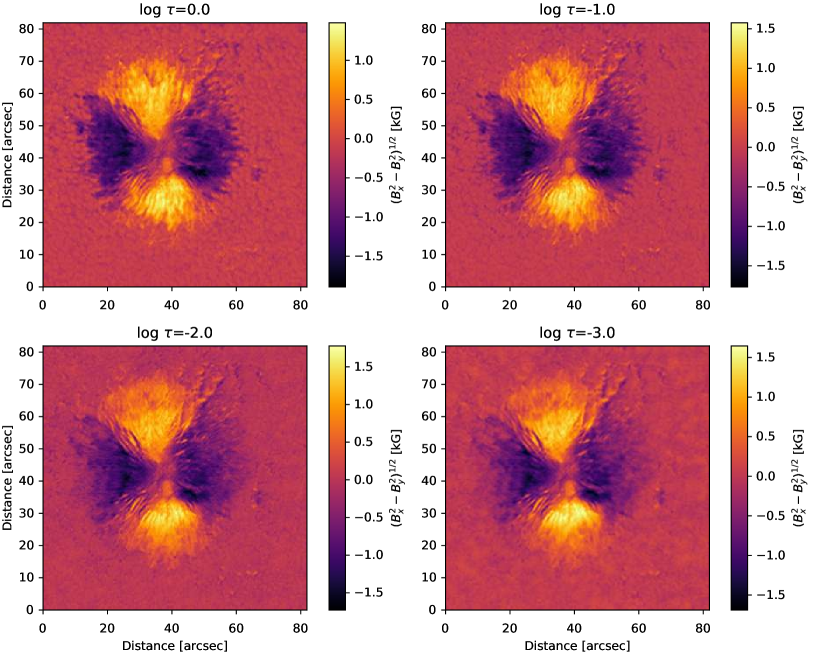
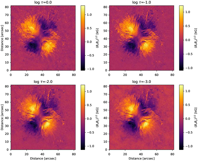
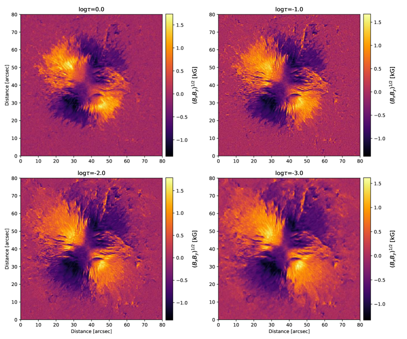
Concerning the magnetic field information, we show $B_{z}$ and the two (signed) combinations of $B_{x}$ and $B_{y}$ that do not suffer from the 180^∘ ambiguity in Fig. 6. The longitudinal field shows very concentrated magnetic field in the darkest regions of the umbra, with a relatively strong (still of the order of 2 kG) hazy structure in the rest of the umbra. The maps inferred by the concatenate networks are slightly more constrasted in $B_{z}$. The surrounding faculae is of opposite polarity and a clumpy ring of opposite polarity surrounds the sunspot, suggesting that the magnetic field is returning back to the photosphere well beyond the penumbral border. The LOS magnetic field in higher layers displays a more diffuse appearance, with field concentrations occupying more area and with weaker fields. The transverse components displays the typical structure with four lobes, rotated by 45^∘ from one component to the other. Appreciable signal is only seen in some parts of the umbra and, fundamentally, on the penumbra. Only some parts of the faculae do show appreciable transverse components of the field. In fact, the expansion of the magnetic field of the sunspot is much better visualized in the transverse component and its variation with height.

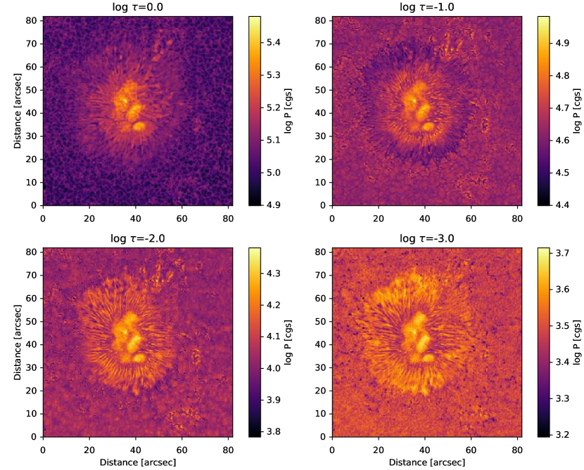
Figure 8 shows the total gas pressure at the same four different optical depth surface. Perhaps one of the most interesting observations is the structure of all magnetic field concentrations away from the sunspot above $\log\tau=0$. The gas pressure at the central part of the magnetized region is roughly equivalent to that of the surrounding quiet Sun at the same optical depth. However, because of the Wilson depression produced by the rarefaction induced by the magnetic field, the radiation is coming from deeper layers. This behavior is different in the borders, with the Wilson depression becoming almost negligible and the total gas pressure strongly increasing until the quiet Sun is reached. This whole picture can be understood as a consequence of a flux tube with a canopy as follows. The central part of the concentration is strongly magnetized so the magnetic pressure is large and the gas pressure is low even if the Wilson depression is large. On the surroundings of the flux tube the magnetic pressure is negligible. In the interface between the two regimes there is still some magnetization which slightly evacuates the plasma and makes it possible to observe deeper layers, where the pressure is larger than in the surrounding quiet Sun.

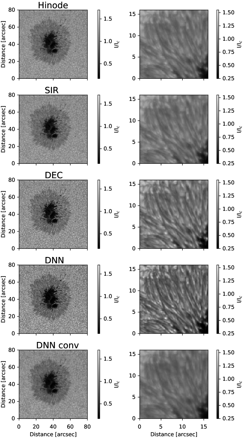
One of the desirable consequences of the neural networks is that the physical quantities in the output are decontaminated from the PSF. This is clearly seen in Fig. 9, where we show continuum images for the whole region (left column) and for a detail in the penumbra (right column). These results are indistinguishable in the two architectures. The root-mean-square contrast, computed as the ratio between the standard deviation and the mean of the brightness in the continuum in a quiet Sun region, is 6.25% for the original Hinode observations. SIR inversions provide a very similar contrast of 6.23%. The contrast obtained after deconvolution goes up to 8.75 %. This contrast can be a little higher if more iterations of the Lucy-Richardson algorithm are applied, but we have preferred to be in the conservative side to avoid introducing artifacts. The contrast obtained from the synthesis in the models inferred from the neural network goes up to 13.58%, very close to the contrast quoted for high-resolution synthetic observations obtained from 3D MHD simulations (e.g., Danilovic et al., 2008). As a test for consistency, when the continuum synthetic image is convolved again with the Hinode PSF, we obtain a contrast of 6.09%.

4.2.1 A complex sunspot

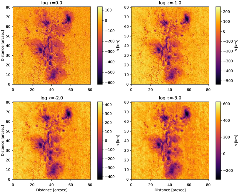
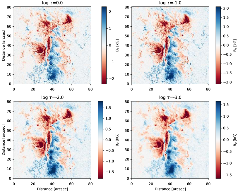
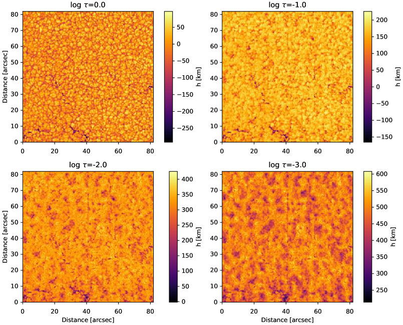
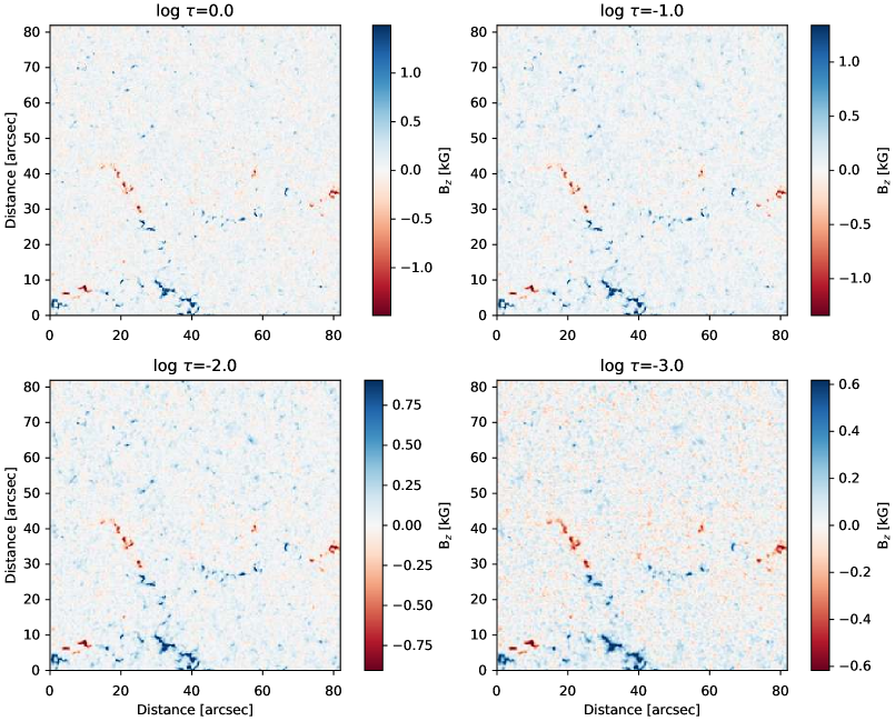
We have also analyzed a much more complex group of sunspots, that correspond to the AR11429. This observation was acquired with Hinode SOT/SP on 2012 March 6 from 22:10 to 22:43 UT. The sunspot is located at coordinates $(-554$″$,-371$″$)$, which corresponds to an heliocentric angle of $\mu=\cos\theta=0.72$. The heliocentric angle is perhaps too large in this case for the results to be quantitatively relevant given that the training set was obtained using only synthesis at disk center. We anticipate that a suitable training set with synthesis carried out at different heliocentric angles could be used to quantitatively analyze observations like this one. The interest of showing this region is to show that the DNN approach can seamlessly be used to infer the physical properties in very complex regions. The Wilson depression and $B_{z}$ are displayed in the upper two rows of Fig. 10 while additional figures with the rest of physical quantities can be found in the repository created for this paper. These Wilson depressions might differ from the real ones when measured perpendicular to the solar surface. Concerning the LOS magnetic field, we find a very complex region with three large-scale polarity inversion lines that are captured by the inversion. Additionally, we find small regions of opposite polarity embedded inside regions of negative polarity.

4.2.2 Quiet Sun

Finally, we show some results with the observation acquired with Hinode SOT/SP on 2007 March 10 from 11:37 to 14:37 UT at disk center. This is a very large portion of the quiet Sun and we only show a small patch of the observation. The results are shown in the lower two rows of Fig. 10. The map of $B_{z}$ displays a large part of the internetwork with very weak fields and a filamentary network structure. The expansion of the field with height is clearly inferred, together with a significant reduction in amplitude. Concerning the Wilson depressions, the $\log\tau=0$ surface on the network is only $\sim$150 km below that of the internetwork. In the internetwork, the Wilson depression for $\log\tau=0$ has a value of $-4.16\pm 37.3$ km, while it becomes $152.9\pm 30.5$ km, $314.5\pm 34.7$ km and $486.5\pm 37.0$ km for $\log\tau=-1$, $\log\tau=-2$ and $\log\tau=-3$, respectively. Consequently, the corrugation of the constant optical depths surfaces is of the order of 35 km in very weakly magnetized regions.

Figure 11: Detailed comparison of results from the neural network approach (in this case with the concatenate architecture) and a standard SIR inversion. We show results for temperature (top three rows), LOS velocity (middle three rows) and longitudinal field (bottom three rows). Inside each set of panels, the top row shows the results of SIR inversions at four selected optical depth heights, the middle row shows the results of SIR inversions after deconvolving the Stokes profiles, while the bottom row shows the results of the neural approach.

4.3 Comparison with standard inversions

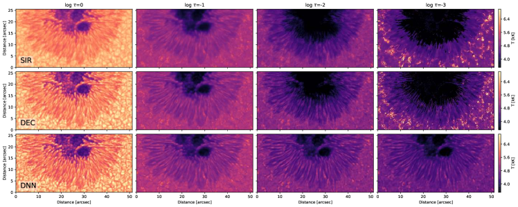
It turns out difficult to compare the output of the neural network with standard inversions because the output of both methods is fundamentally different. In the case of standard SIR inversions, one obtains the average empirical atmosphere that produces a good fit to the profiles in a pixel. In the case of the neural approach, the training was done by injecting the Stokes profiles degraded with the PSF and producing the physical conditions rebinned to the spatial resolution of Hinode. The inferred model atmospheres from both approaches do not need to be either similar or compatible.

Figure 12: Comparison of Stokes $I$ profiles for all considered inversion approaches in five representative pixels. The upper two rows show the results in the encoder-decoder architecture. The lower two rows correspond to the concatenate architecture. The result of the SIR inversion is shown in black dashed line and the inversion obtained with the deconvolved data in black solid line. The profile synthesized in the neural approach is shown in solid color line (in different color for each panel) and the result convolved again with the Hinode PSF in dashed color line.

Figure 13: Like Fig. 12 but for Stokes $V$.

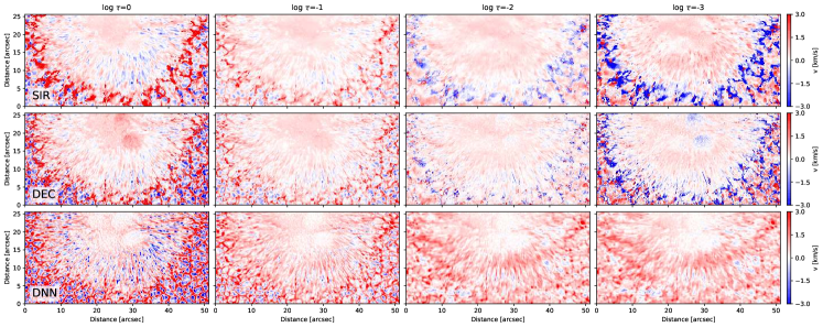
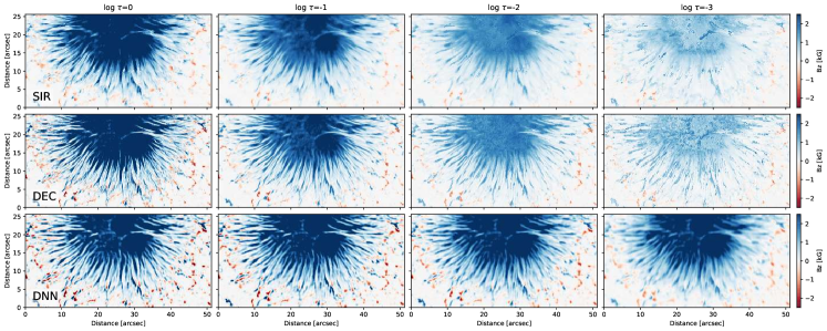
We apply SIR to carry out the inversion of the observed Stokes profiles. We carried out a pixel-by-pixel inversion with an initialization of the inclination of the magnetic field given by the Stokes $V$ polarity ($\theta_{B}=$45^∘ if the blue lobe is positive and $\theta_{B}=$135^∘ otherwise). We choose the Harvard-Smithsonian Reference model Atmosphere (HSRA, Gingerich et al., 1971), covering the optical depth range $-5.0<\log(\tau)<1.4$, as an initial guess atmospheric model. We add a magnetic field strength of 500 G to the initial guess. The inversions were performed in three cycles. The temperature stratification $T(\tau)$ was inverted using 2, 3, and 5 nodes in each cycle, respectively. Two nodes were used for magnetic field strength $B(\tau)$, magnetic field inclination $\theta_{B}(\tau)$, and line-of-sight velocity v$(\tau)$. The magnetic field azimuth $\phi_{B}$ was set constant with height. Although a more complex configuration can be used, we have tried to be conservative as we only have two spectral lines with similar line formation regions. Only partial information about the stratification of the magnetic field can be extracted.

Figure 11 shows a detail in the penumbra for the temperature, LOS velocity and LOS magnetic field. The results obtained with a SIR inversion in the original Hinode profiles are displayed in the upper row, the SIR inversions applied to deconvolved data are displayed in the middle row. Finally, the output of the neural approach (in this case with the concatenate architecture) is displayed in the last row. The increased contrast that we discussed in the continuum images of Fig. 9 is also present in the temperature maps. Filaments are clearly visible in temperature even at $\log\tau=-3$, something that also happens in standard inversions after deconvolution but with a much lower contrast. The salt-and-pepper artifacts in the inversion at higher layers does not appear in the neural approach, which gives a perfectly smooth map given the prior information acquired during the training. Concerning the velocity, we very clearly detect the granulation pattern in deeper regions, which largely disappears at $\log\tau=-3$. In general, we find blueshifts in all the brightest elongated filaments of the penumbra, with redshifts on the laterals, similar to the result of Tiwari et al. (2013). The results are not so clear in the original data inverted with SIR but becomes more conspicuous in the inversions after deconvolution. Finally, the discrepancy between the inversion and the neural network in the LOS magnetic field at higher layers is caused by a combination of the insensitivity of the lines to the field at such heights and to the fact that we are training with a single sunspot. However, it is also important to point out that our approach is more powerful than a pixel-by-pixel inversion because it takes into account the presence of correlation in the spatial and the $\log\tau$ dimensions.

Figure 14: Physical properties displayed in geometric height for a cut at position $X=40^{\prime\prime}$ in the map of the active region AR10933. They have been obtained with the encoder-decoder architecture.

4.4 Synthetic Stokes profiles

It is important to keep in mind that, when neural networks are used for the inversion of Stokes profiles, the resulting physical maps are not forced to fit the profiles like in standard inversion codes. The inversion does not proceed by defining a merit function that measures the misfit between the synthetic Stokes profiles and the observed ones. The network learns an approximate mapping between the Stokes profiles and the physical conditions in an end-to-end supervised manner by minimizing the misfit between the inferred physical conditions and the ones used during training. We have plans to remove this limitation in the near future, as we explain with more detail in Sect. 6.

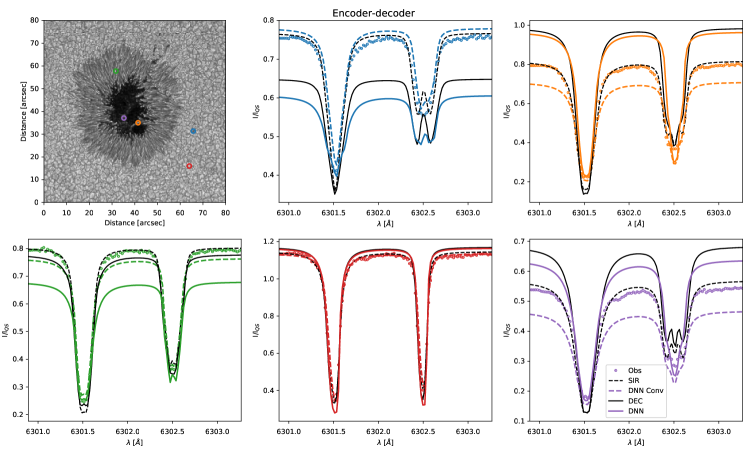
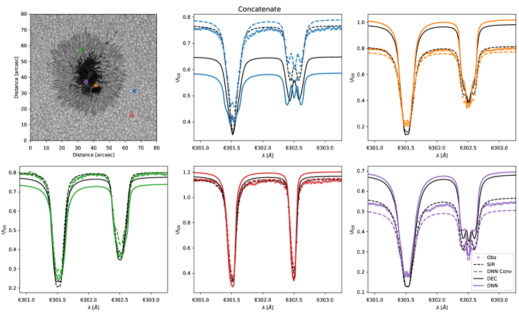
For the moment, we use SIR to synthesize the Stokes profiles emerging from the atmosphere inferred by the neural network and compare it with the original Stokes profiles. To this end we use the inferred maps at the seven optical depth surfaces and generate a smooth model using spline interpolation. This model is then fed to SIR to return the emerging Stokes profiles. We warn the reader that this comparison is somehow misguided and one should not conclude that our results are wrong just because the SIR synthesis in the inferred models does not perfectly fit the observed profiles. This behavior is due to, at least, two reasons. The first one is that the inferred atmospheric model is compensated for the Hinode PSF. This effect is also present in the inversion of the deconvolved data. The second reason is that the neural network is trained to return average atmospheric models per pixel, and we know that the synthetic Stokes profiles in the average model is different from the average of the synthetic Stokes profiles.

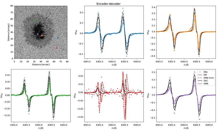
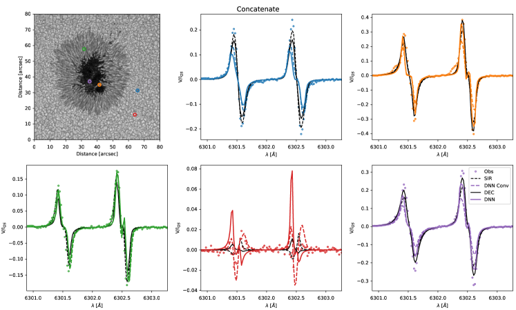
With all these caveats in mind, some examples are displayed in Fig. 12 for Stokes $I$ and in Fig. 13 for Stokes $V$ for five representative pixels and the two architectures. We show the original observation in colored circles, the result of the SIR inversion in black dashed line and the inversion obtained with the deconvolved data in black solid line. The profile synthesized in the neural approach is shown in solid color line (in different color for each panel) and the result convolved again with the Hinode PSF in dashed color line. This figure shows that SIR, by construction, correctly fits the observed profiles. The profiles of the inversion of the deconvolved maps show a much larger contrast (dark regions become darker and bright regions become brigther) as a consequence of the decontamination from the Hinode PSF. The result of the neural networks is very close to this deconvolved result, although it often shows an even larger increase in the contrast. For instance, the location marked in green in the penumbra shows a lower continuum than the observed profile. When the profiles are degraded with the Hinode PSF, we recover a profile that is close to the observation, and also to the standard SIR inversion.

5 Light bridge

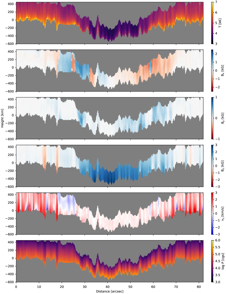
Our ability to recover the inversions in geometric scale allows us to study in detail interesting structures like the light bridge located at coordinates (40″, 35″). To this end, we show a vertical cut at $X=40$″ for some relevant physical quantities in Fig. 14. To generate this plot we interpolate the information provided by the inversion in a common geometric height axis ranging from $-600$ km to 450 km. The vertical cut crosses the light bridge at position $\sim 35$″, roughly in the position of the orange circle in Fig. 12. The Wilson depression for the umbra is larger than $-400$ km on average. On the light bridge the $\log\tau=0$ surface lies at a height of $-200$ km on average and the line formation region spans roughly 250 km in height, so that the $\log\tau=-3$ surface is located at $\sim$50 km. The temperature stratification of the light bridge is closer in structure to that of the quiet Sun or the penumbra, with high temperatures in the lower boundary of $\sim$7000 K. However, slightly lower temperatures are found in the upper layers of the light bridge as compared with those of the quiet Sun. The cusp of the light bridge is found to be slightly redshifted, with very extremely weak blueshifts around, suggesting a weak convection-like motion. Concerning the magnetic field, we find a reduced $B_{z}$ in the cusp, with relatively strong horizontal components of the field in the surroundings of the light bridge. The inferred pressure displays a very good pressure balance in general. Among the exceptions we find the light bridge. It is in a strong pressure imbalance with the surroundings, with differences larger than one order of magnitude. We also find other locations with large imbalances, but are normally associated with strong plasma downflows in intergranular lanes. In general, the behavior of the light bridge is very similar to that found in any penumbra filament, clearly distinct from the surrounding umbra. The global picture of the magnetic structure we obtain is similar to that inferred by Felipe et al. (2016).

6 Conclusions and future work

We have introduced and analyzed an approach for the very fast inference of physical properties from the observation of Stokes profiles leveraging deep learning tools. The case we have discussed is specialized for Hinode observations in the pair of Fe i lines at 630 nm under the assumption of LTE, but we expect applications to other cases to flourish after this work. To this end, we release both the training and evaluation codes as open source so that they can be easily adapted to other applications. The approach has a number of advantages. Firstly, it is extremely fast, especially when used with GPUs. It can invert maps of 512$\times$512 pixels in less than 200 ms using an off-the-shelf GPU. Second, it can easily provide quantities that are very difficult to obtain with normal inversions, like the Wilson depression or the gas pressure. A validation analysis suggests that the neural networks are able to return the physical quantities in a 3D cube with enough precision: temperatures are returned with median deviations below $\pm$82 K, velocities with deviations below $\pm$0.41 km s^-1, heights of the optical depth surfaces with deviations below $\pm$18 km and gas pressure in logarithmic units with deviations around $\pm$0.02 dex. Concerning the magnetic field, we quote deviations that are of the order of or below $\pm$100 G. We point out that the encoder-decoder architecture is able to better exploit the spatial coherence of the physical variables and is slightly less affected by the observational noise. However, although both architectures give good results, in general we find slightly more robust results with the concatenate architecture when applied to Hinode data.

Our approach in this contribution can be understood as a maximum a-posteriori solution to the inversion problem (data-driven priors are introduced by the neural network during training) in which uncertainties are not computed. Obviously, the final aim of any inversion code would be to fully characterize the posterior distribution function for all observed pixels. We anticipate that this will be possible in the near future with the use of machine learning because of the enormous interest in the community of developing interpretable algorithms. Currently, one could argue that the combination of CNNs with their spatial regularization capabilities with recent developments like INNs could be a possible avenue of research. The posterior distributions would surely be multimodal (e.g., Díaz Baso et al., 2019a, b) due to some well-known ambiguities. However, posterior distributions inside each mode tend to be quite well-behaved, nonetheless with the existence of degeneracies (Martínez González et al., 2006; Asensio Ramos et al., 2007a; Asensio Ramos, 2009; Díaz Baso et al., 2019c).

Despite the encouraging results, a caveat is in order. The fact that the neural networks are not explicitly fitting Stokes profiles might be seen problematic. The deep learning approach that we have used here should be considered the first approach to the inversion of Stokes profiles. It is, though, not physically motivated and we are convinced that introducing the radiative transfer (and perhaps also the MHD) physics during training will lead to significant improvements. This requires the introduction of a differentiable forward synthesis module during training. Although we have plans to implement this idea in the near future, we anticipate that the training will become much more time consuming.

Anyway, even if one does not trust the results of the neural networks for doing research, it can always be used as a very high quality initial condition for the application of standard inversion codes. The noise filtering capabilities of the neural network and the exploitation of spatial correlation will allow standard inversion codes to quickly converge to very clean maps. Additionally, the fact that our approach provides the results in geometric height opens up the possibility of using these results with next-generation 3D Stokes inversion including magnetohydrostatic constraints (Pastor Yabar et al., private communication).