Neo: A Learned Query Optimizer

Abstract

Query optimization is one of the most challenging problems in database systems. Despite the progress made over the past decades, query optimizers remain extremely complex components that require a great deal of hand-tuning for specific workloads and datasets. Motivated by this shortcoming and inspired by recent advances in applying machine learning to data management challenges, we introduce Neo (Neural Optimizer), a novel learning-based query optimizer that relies on deep neural networks to generate query executions plans. Neo bootstraps its query optimization model from existing optimizers and continues to learn from incoming queries, building upon its successes and learning from its failures. Furthermore, Neo naturally adapts to underlying data patterns and is robust to estimation errors. Experimental results demonstrate that Neo, even when bootstrapped from a simple optimizer like PostgreSQL, can learn a model that offers similar performance to state-of-the-art commercial optimizers, and in some cases even surpass them.

1 Introduction

In the face of a never-ending deluge of machine learning success stories, every database researcher has likely wondered if it is possible to learn a query optimizer. Query optimizers are key to achieving good performance in database systems, and can speed up the execution time of queries by orders of magnitude. However, building a good optimizer today takes thousands of person-engineering-hours, and is an art only a few experts fully master. Even worse, query optimizers need to be tediously maintained, especially as the system’s execution and storage engines evolve. As a result, none of the freely available open-source query optimizers come close to the performance of the commercial optimizers offered by IBM, Oracle, or Microsoft.

Due to the heuristic-based nature of query optimization, there have been many attempts to improve query optimizers through learning over the last several decades. For example, almost two decades ago, Leo, DB2’s LEarning Optimizer, was proposed [54]. Leo learns from its mistakes by adjusting its cardinality estimations over time. However, Leo still requires a human-engineered cost model, a hand-picked search strategy, and a lot of developer-tuned heuristics, which take years to develop and perfect. Furthermore, Leo only learns better cardinality estimations, but not new optimization strategies (e.g., how to account for uncertainty in cardinality estimates, operator selection, etc.).

More recently, the database community has started to explore how neural networks can be used to improve query optimizers [60, 35]. For example, DQ [22] and ReJOIN [34] use reinforcement learning combined with a human-engineered cost model to automatically learn search strategies to explore the space of possible join orderings. While these papers show that learned search strategies can outperform conventional heuristics on the provided cost model, they do not show a consistent or significant impact on actual query performance. Moreover, they still rely on the optimizer’s heuristics for cardinality estimation, physical operator selection, and estimating the cost of candidate execution plan.

Other approaches demonstrate how machine learning can be used to achieve better cardinality estimates [20, 44, 43]. However, none demonstrate that their improved cardinality estimations actually lead to better query plans. It is relatively easy to improve the average error of a cardinality estimation, but much harder to improve estimations for the cases that actually improve query plans [26]. Furthermore, cardinality estimation is only one component of an optimizer. Unlike join order selection, identifying join operators (e.g., hash join, merge join) and selecting indexes cannot be (entirely) reduced to cardinality estimation. Finally, SkinnerDB showed that adaptive query processing strategies can benefit from reinforcement learning, but requires a specialized query execution engine, and cannot benefit from operator pipelining or other advanced parallelism models [56].

In other words, none of the recent machine-learning-based approaches come close to learning an entire optimizer, nor do they show how their techniques can achieve state-of-the-art performance (to the best of our knowledge, none of these approaches compare with a commercial optimizer). Showing that an entire optimizer can be learned remains an important milestone and has far reaching implications. Most importantly, if a learned query optimizer could achieve performance comparable to commercial systems after a short amount of training, the amount of human development time to create a new query optimizer will be significantly reduced. This, in turn, will make good optimizers available to a much broader range of systems, and could improve the performance of thousands of applications that use open-source databases today. Furthermore, it could change the way query optimizers are built, replacing an expensive stable of heuristics with a more holistic optimization problem. This should result in better maintainability, as well as lead to optimizers that will truly learn from their mistakes and adjust their entire strategy for a particular customer instance to achieve instance optimality [21].

In this work, we take a significant step towards the milestone of building an end-to-end learned optimizer with state-of-the-art performance. To the best of our knowledge, this work is the first to show that an entire query optimizer can be learned. Our learned optimizer is able to achieve similar performance to state-of-the-art commercial optimizers, e.g., Oracle and Microsoft, and sometimes even surpass them. This required overcoming several key challenges, from capturing query semantics as vectors, processing tree-based query plan structures, designing a search strategy, incorporating physical operator and index selection, replacing human-engineered cost models with a neural network, adopting reinforcement learning techniques to continuously improve, and significantly shorting the training time for a given database. All these techniques were integrated into the first end-to-end learned query optimizer, called Neo (Neural Optimizer).

Neo learns to make decisions about join ordering, physical operator selection, and index selection. However, we have not yet reached the milestone of learning these tasks from scratch. First, Neo still requires a-priori knowledge about all possible query rewrite rules (this guarantees semantic correctness and the number of rules are usually small). Second, we restrict Neo to project-select-equijoin-aggregate-queries (though, our framework is general and can easily be extended). Third, our optimizer does not yet generalize from one database to another, as our features are specific to a set of tables — however, Neo does generalize to unseen queries, which can contain any number of known tables. Fourth, Neo requires a traditional (weaker) query optimizer to bootstrap its learning process. As proposed in [35], we use the traditional query optimizer as a source of expert demonstration, which Neo uses to bootstrap its initial policy. This technique, referred to as “learning from demonstration” [49, 16, 9, 50] significantly speeds up the learning process, reducing training time from days/weeks to just a few hours. The query optimizer used to bootstrap Neo can be much weaker in performance and, after an initial training period, Neo surpasses its performance and it is no longer needed. For this work, we use the PostgreSQL optimizer, but any traditional (open source) optimizer can be used.

Our results show that Neo outperforms commercial optimizers on their own query execution engines, even when it is boostrapped using the PostgreSQL optimizer. Interestingly, Neo learns to automatically adjust to changes in the accuracy of cardinality predictions (e.g., it picks more robust plans if the cardinality estimates are less precise). Further, it can be tuned depending on the customer preferences (e.g., increase worst-case performance vs. relative performance) — adjustments which are hard to achieve with traditional techniques.

We argue that Neo represents a step forward in building an entirely learned optimizer. Moreover, Neo can already be used, in its current form, to improve the performance of thousands of applications which rely on PostgreSQL and other open-source database systems (e.g. SQLite). We hope that Neo inspires many other database researchers to experiment with combining query optimizers and learned systems in new ways, similar to how AlexNet [23] changed the way image classifiers were built.

In summary, we make the following contributions:

• We propose Neo  — an end-to-end learning approach to query optimization, including join ordering, index selection, and physical operator selection.

• We show that, after training for a dataset and representative sample query workload, Neo is able to generalize even over queries it has not encountered before.

• We evaluate different feature engineering techniques and propose a new technique, which implicitly represents correlations within the dataset.

• We show that, after a short amount of training, Neo is able to achieve performance comparable to Oracle’s and Microsoft’s query optimizers on their respective database systems.

The remainder of the paper is organized as follows: Section 2 provides an overview of Neo’s learning framework and system model. Section 3 describes how queries and query plans are represented by Neo. Section 4 explains Neo’s value network, the core learned component of our system. Section 5 describes row vector embeddings, an optional learned representation of the underlying database that helps Neo understand correlation within the user’s data. We present an experimental evaluation of Neo in Section 6, discuss related works in Section 7, and offer concluding remarks in Section 8.

	Traditional Optimizer	Neural Optimizer (Neo)
Creation	Human developers	Demonstration, reinforcement learning (Section 2)
Query Representation	Operator tree	Feature encoding (Section 3)
Cost Model	Hand-crafted model	Learned DNN model (Section 4)
Plan Space Enumeration	Heuristics, dynamic programming	DNN-guided search strategy (Section 4.2)
Cardinality Estimation	Histograms, hand-crafted models	Histograms, learned embeddings (Section 5)

Table 1: Traditional cost-based query optimizer vs. Neo

2 Learning Framework Overview

What makes Neo unique that it is the very first end-to-end query optimizer. As shown in Table 1, it replaces every component of a traditional Selinger-style [52] query optimizers through machine learning models: (i) the query representation is through features rather than an object-based query operator tree (e.g., Volcano-style [15] iterator tree); (ii) the cost model is a deep neural network (DNN) model as opposed to hand-crafted equations; (iii) the search strategy is a DNN-guided learned best-first search strategy instead of plan space enumeration or dynamic programming; (iv) cardinality estimation is based on either histograms or a learned vector embedding scheme, combined with a learned model, instead of hand-tuned histogram-based cardinality estimation model. Finally, (v) Neo uses reinforcement learning and learning from demonstration to integrate these into an end-to-end query optimizer rather than relying on human engineering. While we describe the different components in the individual sections as outlined in Table 1, the following provides a general overview of how Neo learns, as depicted in Figure 1.

Figure 1: Neo system model

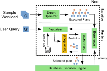
Expertise Collection The first phase, labeled Expertise, initially generates experience from a traditional query optimizer, as proposed in [35]. Neo assumes the existence of an application-provided Sample Workload consisting of queries representative of the application’s total workload. Additionally, we assume Neo has access to a simple, traditional rule- or cost-based Expert Optimizer (e.g., Selinger [52], PostgreSQL [1]). This simple optimizer is treated as a black box, and is only used to create query execution plans (QEPs) for each query in the sample workload. These QEPs, along with their latencies, are added to Neo’s Experience (i.e., a set of plan/latency pairs), which will be used as a starting point in the next model training phase. Note that the Expert Optimizer can be unrelated to the underlying Database Execution Engine.

Model Building Given the collected experience, Neo builds an initial Value Model. The value model is a deep neural network with an architecture designed to predict the final execution time of a given partial or complete plan for a given query. We train the value network using the collected experience in a supervised fashion. This process involves transforming each user-submitted query into features (through the Featurizer module) useful for a machine learning model. These features contain both query-level information (e.g., the join graph, predicated attributes, etc.) and plan-level information (e.g., selected join order, access paths, etc.). Neo can work with a number of different featurization techniques, ranging from simple one-hot encodings (Section 3) to more complex embeddings (Section 5). Neo’s value network uses tree convolution [40] to process the tree-structured QEPs (Section 4.1).

Plan Search Once query-level information has been encoded, Neo uses the value model to search over the space of QEPs (i.e., selection of join orderings, join operators, and indexes) and discover the plan with the minimum predicted execution time (i.e., value). Since the space of all execution plans for a particular query is far too large to exhaustively search, Neo performs a best-first search of the space, using the value model as a heuristic. A complete plan created by Neo, which includes a join ordering, join operators (e.g. hash, merge, loop), and access paths (e.g., index scan, table scan) is sent to the underlying execution engine, which is responsible for applying semantically-valid query rewrite rules (e.g., inserting necessary hash and sort operations) and executing the final plan. This ensures that every execution plan generated by Neo computes the correct result. The plan search is discussed in detail in Section 4.2.

Model Refinement As new queries are optimized through Neo, the model is iteratively improved and custom-tailored to the underlying database and execution engine. This is achieved by incorporating newly collected experience regarding each query’s QEP and performance. Specifically, once a QEP is chosen for a particular query, it is sent to the underlying execution engine, which processes the query and returns the result to the user. Additionally, Neo records the final execution latency of the QEP, adding the plan/latency pair to its Experience. Then, Neo retrains the value model based on this experience, iteratively improving its estimates.

Discussion This process – featurizing, searching, and refining – is repeated for each query sent by the user. Neo’s architecture is designed to create a corrective feedback loop: when Neo’s learned cost model guides Neo to a query plan that Neo predicts will perform well, but then the resulting latency is high, Neo’s cost model learns to predict a higher cost for the poorly-performing plan. Thus, Neo is less likely to choose plans with similar properties to the poorly-performing plan in the future. As a result, Neo’s cost model becomes more accurate, effectively learning from its mistakes.

Neo’s architecture, of using a learned cost model to guide a search through a large and complex space, is inspired by AlphaGo [53], a reinforcement learning system developed to play the game of Go. At a high level, for each move in a game of Go, AlphaGo uses a neural network to evaluate the desirability of each potential move, and uses a search routine to find a sequence of moves that is most likely to lead to a winning position. Similarly, Neo uses a neural network to evaluate the desirability of partial query plans, and uses a search function to find a complete query plan that is likely to lead to lower latency.

Both AlphaGo and Neo additionally bootstrap their cost models from experts. AlphaGo bootstraps from a dataset of Go games played by expert humans, and Neo bootstraps from a dataset of query execution plans built by a traditional query optimizer (which was designed by human experts). The reason for this bootstrapping is because of reinforcement learning’s inherent sample inefficiency [16, 49]: without bootstrapping, reinforcement learning algorithms like Neo or AlphaGo may require millions of iterations [38] before even becoming competitive with human experts. Bootstrapping from an expert source (i.e., learning from demonstration) intuitively mirrors how young children acquire language and learn to walk by imitating nearby adults (experts), and has been shown to drastically reduce the number of iterations required to learn a good policy [16, 50]. Decreasing sample inefficiency is especially critical for database management systems: each iteration requires a query execution, and users are unlikely to be willing to execute millions of queries before achieving performance on-par with current query optimizers. Worse yet, executing a poor query execution plan takes longer than executing a good execution plan, so the initial iterations would take an infeasible amount of time to complete [35].

Thus, Neo can be viewed as a learning-from-demonstration reinforcement learning system similar to AlphaGo – there are, however, many differences between AlphaGo and Neo. First, because of the grid-like nature of the Go board, AlphaGo can trivially represent the board as an image and use image convolution, possibly the most well-studied and highly-optimized neural network primitive [28, 24], in order to predict the desirability of a board state. On the other hand, query execution plans have a tree structure, and cannot be trivially represented as images, nor can image convolution be easily applied. Second, in Go, the board represents all the information relevant to a particular move, and can be represented using less than a kilobyte of storage. In query optimization, the data in the user’s database is highly relevant to the performance of query execution plans, and is generally much larger than a kilobyte (it is not possible to simply feed a user’s entire database into a neural network). Third, AlphaGo has a single, unambiguous goal: defeat its opponent and reach a winning game state. Neo, on the other hand, needs to take the user’s preferences into account, e.g. should Neo optimize for average-case or worst-cast latency?

The remainder of this paper describes our solutions to these problems in detail, starting with the notation and encoding of the query plans.

3 Query Featurization

In this section, we describe how query plans are represented as vectors, starting with some necessary notation.

3.1 Notation

For a given query $q$, we define the set of base relations used in $q$ as $R(q)$. A partial execution plan $P$ for a query $q$ (denoted $Q(P)=q$) is a forest of trees representing an execution plan that is still being built. Each internal (non-leaf) tree node is a join operator $\bowtie_{i}\in J$, where $J$ is the set of possible join operators (e.g., hash join $\bowtie_{H}$, merge join $\bowtie_{M}$, loop join $\bowtie_{L}$) and each leaf tree node is either a table scan, an index scan, or an unspecified scan over a relation $r\in R(q)$, denoted $T(r)$, $I(r)$, and $U(r)$ respectively. An unspecified scan is a scan that has not been assigned as either a table or an index scan yet. For example, the partial query execution plan depicted in Figure 2 is denoted as:

$$\left[(T(D)\bowtie_{M}T(A))\bowtie_{L}I(C)\right],\quad\left[U(B)\right]$$

Figure 2: Partial query plan

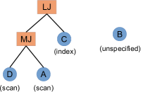
Here, the type of scan for $B$ is still unspecified, as is the join that will eventually link $B$ with the rest of the plan, but the plan specifies a table scan of table $D$ and $A$, which feed into a merge join, whose result will then be joined using a loop join with $C$.

A complete execution plan is a plan with only a single tree and with no unspecified scans; all decisions on how the plan should be executed have been made. We say that one execution plan $P_{i}$ is a subplan of another execution plan $P_{j}$, written $P_{i}\subset P_{j}$, if $P_{j}$ could be constructed from $P_{i}$ by (1) replacing unspecified scans with index or table scans, and (2) combining subtrees in $P_{i}$ with a join operator.

3.2 Encodings

In order to train a neural network to predict the final latency of partial or complete query execution plans (QEPs), we require two encodings: first, a query encoding, which encodes information regarding the query, but is independent of the query plan. For example, the involved tables and predicates fall into this category. Second, we require a plan encoding, which represents the partial execution plan.

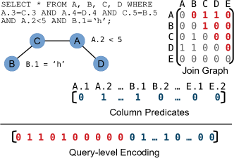
Query Encoding The representation of query-dependent but plan-independent information in Neo is similar to the representations used in previous work [22, 34], and consists of two components. The first component encodes the joins performed by the query, which can be represented as an adjacency matrix of the join graph, e.g. in Figure 3, the 1 in the first row, third column corresponds to the join predicate connecting A and C. Both the row and column corresponding to the relation $E$ are empty, because $E$ is not involved in the example query. Here, we assume that at most one foreign key between each relation exists. However, the representation can easily be extended to include more than one potential foreign key (e.g., by using the index of the relevant key instead of the constant value “1”, or by adding additional columns for each foreign key). Furthermore, since this matrix is symmetrical, we choose only to encode the upper triangular portion, colored in red in Figure 3. Note that the join graph does not specify the order of joins.

The second component of the query encoding is the column predicate vector. In Neo, we currently support three increasingly powerful variants, with varying levels of precomputation requirements:

Figure 3: Query-level encoding

Figure 4: Plan-level encoding

1. 1-Hot (the existence of a predicate): is a simple “one-hot” encoding of which attributes are involved in a query predicate. The length of the one-hot encoding vector is the number of attributes over all database tables. For example, Figure 3 shows the “one-hot” encoded vector with the positions for attribute $A.2$ and $B.1$ set to 1, since both attributes are used as part of predicate. Note that join predicates are not considered here. Thus, the learning agent only knows whether an attribute is present in a predicate or not. While naive, the 1-Hot representation can be built without any access to the underlying database.

2. Histogram (the selectivity of a predicate): is a simple extension of the previous one-hot encoding which replaces the indication of a predicate’s existence with the predicted selectivity of that predicate (e.g., $A.2$ could be $0.2$, if we predict a selectivity of $20\%$). For predicting selectivity, we use an off-the-shelf histogram approach with uniformity assumptions, as used by PostgreSQL and other open-source systems.

3. R-Vector (the semantics of a predicate): is the most advanced encoding scheme, where we use row vectors. We designed row vectors based on a natural language processing (NLP) model mirroring word vectors [36]. In this case, each entry in the column predicate vector contains semantically relevant information related to the predicate. This encoding requires building a model over the data in the database, and is the most expensive option. We discuss row vectors in Section 5.

The more powerful the encoding, the more degrees of freedom the model has to learn complex relationships. However, this does not necessarily mean that the model cannot learn more complex relationships with a simpler encoding. For example, even though Histogram does not encode anything about correlations between tables, the model might still learn about them and accordingly correct the cardinality estimations internally, e.g. from repeated observation of query latencies. However, with the R-Vector encoding, we make Neo’s job easier by providing a semantically-enhanced representation of the query predicate.

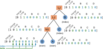
Plan Encoding The second encoding we require is to represent the partial or complete query execution plan. While prior works [22, 34] have flattened the tree structure of each partial execution plan, our encoding preserves the inherent tree structure of execution plans. We transform each node of the partial execution plan into a vector, creating a tree of vectors, as shown in Figure 4. While the number of vectors (i.e., number of tree nodes) can increase, and the structure of the tree itself may change (e.g., left deep or bushy), every vector has the same number of columns.

These vectors are created as follows: each node is transformed into a vector of size $|J|+2|R|$, where $|J|$ is the number of different join operators, and $|R|$ is the number of relations. The first $|J|$ entries of each vector encode the join type (e.g., in Figure 4, the root node uses a loop join), and the next $2|R|$ entries encode which relations are being used, and what type of scan (table, index, or unspecified) is being used. For leaf nodes, this subvector is a one-hot encoding, unless the leaf represents an unspecified scan, in which case it is treated as though it were both an index scan and a table scan (a 1 is placed in both the “table” and “index” columns). For any other node, these entries are the union of the corresponding children nodes. For example, the bottom-most loop join operator in Figure 4 has ones in the position corresponding to table scans over D and A, and an index scan over C.

Note that this representation can contain two partial query plans (i.e., several roots) which have yet to be joined, e.g. to represent the following partial plan:

$$P=\left[(T(D)\bowtie_{M}T(A))\bowtie_{L}I(C)\right],\quad\left[U(B)\right]$$

When encoded, the $U(B)$ root node would be encoded as:

$$[0000110000]$$

Intuitively, partial execution plans are built “bottom up”, and partial execution plans with multiple roots represent subplans that have yet to be joined together with a join operator. The purpose of these encodings is merely to provide a representation of execution plans to Neo’s value network, described next.

4 Value Network

Figure 5: Value network architecture

In this section, we present the Neo value network, a deep neural network model which is trained to approximate the best-possible query latency that a partial execution plan $P_{i}$ could produce (in other words, the best-possible query latency achievable by a complete execution plan $P_{f}$ such that $P_{i}$ is a subplan of $P_{f}$). Since knowing the best-possible complete execution plan for a query ahead of time is impossible (if it were possible, the need for a query optimizer would be moot), we approximate the best-possible query latency with the best query latency seen so far by the system.

Formally, let Neo’s experience $E$ be a set of complete query execution plans $P_{f}\in E$ with known latency, denoted $L(P_{f})$. We train a neural network model $M$ to approximate, for all $P_{i}$ that are a subplan of any $P_{f}\in E$:

$$M(P_{i})\approx\min\{C(P_{f})\mid P_{i}\subset P_{f}\land P_{f}\in E\}$$

where $C(P_{f})$ is the cost of a complete plan. The user can change the cost function to alter the behavior of Neo. For example, if the user is concerned only with minimizing total query latency across the workload, the cost could be defined as the latency, i.e.,

$$C(P_{f})=L(P_{f}).$$

However, if instead the user prefers to ensure that every query $q$ in a workload performs better than a particular baseline, the cost function can be defined as

$$C(P_{f})=L(P_{f})/Base(P_{f}),$$

where $Base(P_{f})$ is latency of plan $P_{f}$ with that baseline. Regardless of how the cost function is defined, Neo will attempt to minimize it over time. We experimentally evaluate both of these cost functions in Section 6.4.4.

The model is trained by minimizing a loss function [51]. We use a simple L2 loss function:

$$(M(P_{i})-\min\{C(P_{f})\mid P_{i}\subset P_{f}\land P_{f}\in E\})^{2}.$$

Network Architecture The architecture of the Neo value network model is shown in Figure 5. We designed the model’s architecture to create an inductive bias [33] suitable for query optimization: the structure of the neural network itself is designed to reflect an intuitive understanding of what causes query plans to be fast or slow. Intuitively, humans studying query plans learn to recognize suboptimal or good plans by pattern matching: a merge join on top of a hash join with a shared join key is likely inducing a redundant sort or hash step; a loop join on top of two hash joins is likely to be highly sensitive to cardinality estimation errors; a hash join using a fact table as the “build” relation is likely to incur spills; a series of merge joins that do not require re-sorting is likely to perform well, etc. Our insight is that all of these patterns can be recognized by analyzing subtrees of a query execution plan. Our model architecture is essentially a large bank of these patterns that are learned automatically, from the data itself, by taking advantage of a technique called tree convolution [40] (discussed in Section 4.1).

As shown in Figure 5, when a partial query plan is evaluated by the model, the query-level encoding is fed through a number of fully-connected layers, each decreasing in size. The vector outputted by the third fully connected layer is concatenated with the plan-level encoding, i.e., each tree node (the same vector is added to all tree nodes). This is a standard technique [53] known as “spatial replication” [63] for combining data that has a fixed size (the query-level encoding) and data that is dynamically sized (the plan-level encoding). Once each tree node vector has been augmented, the forest of trees is sent through several tree convolution layers [40], an operation that maps trees to trees. Afterwards, a dynamic pooling operation [40] is applied, flattening the tree structure into a single vector. Several additional fully connected layers are used to map this vector into a single value, used as the model’s cost prediction for the inputted execution plan. A formal description of the value network model is given in Appendix A.

4.1 Tree Convolution

Figure 6: Tree convolution examples

Common neural network models, like fully-connected neural networks or convolution neural networks, take as input tensors with a fixed structure, such as a vector or an image. In our problem, the features embedded in each execution plan are structured as nodes in a query plan tree (e.g., Figure 4). To process these features, we use tree convolution methods [40], an adaption of traditional image convolution for tree-structured data.

Tree convolution is a natural fit for this problem. Similar to the convolution transformation for images, tree convolution slides a set of shared filters over each part of the query tree locally. Intuitively, these filters can capture a wide variety of local parent-children relations. For example, filters can look for hash joins on top of merge joins, or a join of two relations when a particular predicate is present. The output of these filters provides signals utilized by the final layers of the value network; filter outputs could signify relevant factors such as when the children of a join operator are sorted on the key (in which case merge join is likely a good choice), or a filter might estimate if the right-side relation of a join will have low cardinality (indicating that an index may be useful). We provide two concrete examples later in this section.

Operationally, since each node on the query tree has exactly two child nodes, each filter consists of three weight vectors, $e_{p},e_{l},e_{r}$. Each filter is applied to each local “triangle” formed by the vector $x_{p}$ of a node and two of its left and right child, $x_{l}$ and $x_{r}$ to produce a new tree node $x_{p}^{\prime}$:

$$x_{p}^{\prime}=\sigma(e_{p}\odot x_{p}+e_{l}\odot x_{l}+e_{r}\odot x_{r}).$$

Here, $\sigma(\cdot)$ is a non-linear transformation (e.g., ReLU [14]), $\odot$ is a dot product, and $x_{p}^{\prime}$ is the output of the filter. Each filter thus combines information from the local neighborhood of a tree node (its children). The same filter is “slid” across each tree in a execution plan, allowing a filter to be applied to execution plans with arbitrarily sized trees. A set of filters can be applied to a tree in order to produce another tree with the same structure, but with potentially different sized vectors representing each node. In a large neural network, such as those in our experimental evaluation, typically hundreds of filters are applied.

Since the output of a tree convolution is also a tree with the same shape as the input (but with different sized vector representing each node), multiple layers of tree convolution filters can be sequentially applied to an execution plan. The first layer of tree convolution filters will access the augmented execution plan tree, and each filter will “see” each parent/left child/right child triangle of the original tree. The amount of information seen by a particular filter is called the filter’s receptive field [30]. The second layer of convolution filters will be applied to the output of the first, and thus each filter in this second layer will see information derived from a node $n$ in the original augmented tree, $n$’s children, and $n$’s grandchildren. Thus, each tree convolution layer has a larger receptive field than the last. As a result, the first tree convolution layer will learn simple features (e.g., recognizing a merge join on top of a merge join), whereas the last tree convolution layer will learn complex features (e.g., recognizing a left-deep chain of merge joins).

We present two concrete examples in Figure 6 that show how the first layer of tree convolution can detect interesting patterns in query execution plans. In Example 1 of Figure 6a, we show two execution plans that differ only in the topmost join operator (a merge join and hash join). As depicted in the the top portion of Figure 6b, the join type (hash or merge) is encoded in the first two bits of the feature vector in each node. Now, if a tree convolution filter (Figure 6c top) is comprised of three weight vectors with $\{1,-1\}$ in the first two positions and zeros for the rest, it will serve as a “detector” for query plans with two merge joins in a row. This can be seen in Figure 6d (top): the root node of the plan with two merge joins in a row receives an output of 2 from this filter, whereas the root node of the plan with a hash join on top of a merge join receives an output of 0. Subsequent tree convolution layers can use this information to form more complex predicates, e.g. to detect three merge joins in a row (a pipelined query execution plan), or a mixture of merge joins and hash joins (which may require frequent re-hashing or re-sorting). In Example 2 of Figure 6, suppose A and B are physically sorted on the same key, and are thus optimally joined together with a merge join operator, but that C is not physically sorted. The tree convolution filter shown in Figure 6(c, bottom) serves as a detector for query plans that join A and B with a merge join, behavior that is likely desirable. The top weights recognize the merge join ({1, -1} for the first two entries) and the right weights prefer table B over all other tables. The result of this convolution (Figure 6d bottom) shows its highest output for the merge join of A and B (in the first plan), and a negative output for the merge join of A and C (in the second plan).

In practice, filter weights are learned over time in an end-to-end fashion. By using tree convolution layers in a neural network, performing gradient descent on the weights of each filter will cause filters that correlate with latency (e.g., helpful features) to be rewarded (remain stable), and filters with no clear relationship to latency to be penalized (pushed towards more useful values). This creates a corrective feedback loop, resulting in the development of filterbanks that generate useful features [28].

4.2 DNN-Guided Plan Search

The value network predicts the quality (cost) of an execution plan, but it does not directly give an execution plan. Following several recent works in reinforcement learning [53, 2], we combine the value network with a search technique to generate query execution plans, resulting in a value iteration technique [5] (discussed at the end of the section).

Given a trained value network and an incoming query $q$, Neo performs a search of the plan space for a given query. Intuitively, this search mirrors the search process used by traditional database optimizers, with the trained value network taking on the role of the database cost model. Unlike these traditional systems, the value network does not predict the cost of a subplan, but rather the best possible latency achievable from an execution plan that includes a given subplan. This difference allows us to perform a best-first search [10] to find an execution plan with low expected cost. Essentially, this amounts to repeatedly exploring the candidate with the best predicated cost until a halting condition occurs.

The search process for query $q$ starts by initializing an empty min heap to store partial execution plans. This min heap is ordered by the value network’s estimation of a partial plan’s cost. Then, a partial execution plan with an unspecified scan for each relation in $R(q)$ is added to the heap. For example, if $R(q)=\{A,B,C,D\}$, then the heap is initialized with $P_{0}$:

$$P_{0}=[U(A)],\quad[U(B)],\quad[U(C)],\quad[U(D)],$$

where $U(r)$ is the unspecified scan for the relation $r\in R(q)$.

At each search iteration, the subplan $P_{i}$ at the top of the min heap is removed. We enumerate all of $P_{i}$’s children, $Children(P_{i})$, scoring them using the value network and adding them to the min heap. Intuitively, the children of $P_{i}$ are all the plans creatable by specifying a scan in $P_{i}$ or by joining two trees of $P_{i}$ with a join operator. Formally, we define $Children(P_{i})$ as the empty set if $P_{i}$ is a complete plan, and otherwise as all possible subplans $P_{j}$ such that $P_{i}\subset P_{j}$ and such that $P_{j}$ and $P_{i}$ differ by either (1) changing an unspecified scan to a table or index scan, or (2) merging two trees using a join operator. Once each child is scored and added to the min heap, another search iteration begins, resulting in the next most promising node being removed from the heap and explored.

While one could terminate this search process as soon as a leaf node (a complete execution plan) is found, this search procedure can easily be transformed into an anytime search algorithm [64], i.e. an algorithm that continues to find better and better results until a fixed time cutoff. In this variant, the search process continues exploring the most promising nodes from the heap until a time threshold is reached, at which point the most promising complete execution plan is returned. This gives the user control over the tradeoff between planning time and execution time. Users could even select a different time cutoff for different queries depending on their needs. In the event that the time threshold is reached before a complete execution plan is found, Neo’s search procedure enters a “hurry up” mode [55], and greedily explores the most promising children of the last node explored until a leaf node is reached. The cutoff time should be tuned on a per-application bases, but we find that a value of 250ms is sufficient for a wide variety of workloads (see Section 6.5), a value that is acceptable for many applications.

From a reinforcement learning point of view, the combination of the value network with a search procedure is a value iteration technique [5]. Value iteration techniques cycle between two steps: estimating the value function, and then using that value function to improve the policy. We estimate the value function via supervised training of a neural network, and we use that value function to improve a policy via a search technique. Q learning [61] and its deep neural network variants [38], which have been recently used for query optimization [22], are also value iteration methods: the value estimation step is similar, but they use that value function to select actions greedily (i.e., without a search). This approach is equivalent to Neo’s “hurry up” mode. As our experiments show, combining value estimation with a search procedure leads to a system that is less sensitive to noise or inaccuracies in the value estimation model, resulting in significantly better query plans. This improvement has been observed in other fields as well [53, 2].

5 Row Vector Embeddings

Neo can represent query predicates in a number of ways, including a simple one-hot encoding (1-Hot) or a histogram-based representation (Histogram), as described in Section 3. Here, we motivate and describe row vectors, Neo’s most advanced option for representing query predicates (R-Vector).

Cardinality estimation is one of the most important problems in query optimization today [29, 25]. Estimating cardinalities is directly related to estimating selectivities of query predicates – whether these predicates involve a single table or joins across multiple tables. The more columns or joins are involved, the harder the problem becomes. Modern database systems make several simplifying assumptions about these correlations, such as uniformity, independence, and/or the principle of inclusion [26]. These assumptions often do not hold in real-world workloads, causing orders of magnitude increases in observed query latencies [25]. In Neo, we take a different approach: instead of making simplifying assumptions about data distributions and attempting to directly estimate predicate cardinality, we build a semantically-rich, vectorized representation of query predicates that can serve as an input to Neo’s value model, enabling the network to learn generalizable data correlations.

While Neo supports several different encodings for query predicates, here we present row vectors, a new technique based on the popular word2vec [36] algorithm. Intuitively, we build a vectorized representation of each query predicate based on data in the database itself. These vectors are meaningless on their own, but the distances between these vectors will have semantic meaning. Neo’s value network can take these row vectors are inputs, and use them to identify correlations within the data and predicates with syntactically-distinct but semantically-similar values (e.g. $Genre$ is “action” and $Genre$ is “adventure”).

5.1 R-Vector Featurization

The basic idea behind our approach is to capture contextual cues among values that appear in a database. To give a high-level example from the IMDB movie dataset [25], if a keyword “marvel-comics” shows up in a query predicate, then we wish to be able to predict what else in the database would be relevant for this query (e.g., other Marvel movies).

Word vectors To generate row vectors, we use word2vec — a natural language processing technique for embedding contextual information about collections of words [36]. In the word2vec model, each sentence in a large body of text is represented as a collection of words that share a context, where similar words often appear in similar contexts. These words are mapped to a vector space, where the angle and distance between vectors reflect the similarity between words. For example, the words “king” and “queen” will have similar vector representations, as they frequently appear in similar contexts (e.g. “Long live the…”), whereas words like “oligarch” and “headphones” will have dissimilar vector representations, as they are unlikely to appear in similar contexts.

We see a natural parallel between sentences in a document and rows in a database: values of correlated columns tend to appear together in a database row. In fact, word2vec-based embeddings have recently been applied to other database problems, such as semantic querying [7], entity matching [41], and data discovery [12]. In Neo, we use an off-the-shelf word2vec implementation [48] to build an embedding of each value in the database. We then utilize these embeddings to encode correlations across columns.

We explored two variants of this featurization scheme. In the first approach, we treat each row in every table of the database as a training sentence. This approach captures correlations within a table. To better capture cross-table correlations, in our second approach, we augment the set of training sentences by partially denormalizing the database. Concretely, we join large fact tables with smaller tables which share a foreign key, and each resulting row becomes a training sentence. Denormalization enables learning correlations such as “Actors born in Paris are more likely to play in French movies”. While a Paris-born actor’s name and birthplace may be stored only in the names table, the cast_info table captures information relating this actor to many French movies. By joining these two tables together, we can make these relationships — such as the actor’s name, birthplace, and all the French movies they have appeared in — explicit to the word2vec training algorithm. Conceptually, denormalizing the entire database would provide the best embedding quality, but at the expense of significantly increasing the size and number of training examples (a completely denormalized database may have trillions of rows), and hence the word2vec training time. A fully denormalized database is often unfeasible to materialize. In Section 6.3.2, we present the details of the row vector training performance in practice. Our word2vec training process is open source, and available on GitHub.

(a) Birthplace of each actor

(b) Top actors in each genre

Figure 7: t-SNE projection of actor names embedded in the word2vec model. Column correlations across multiple IMDB tables show up as semantically meaningful clusters.

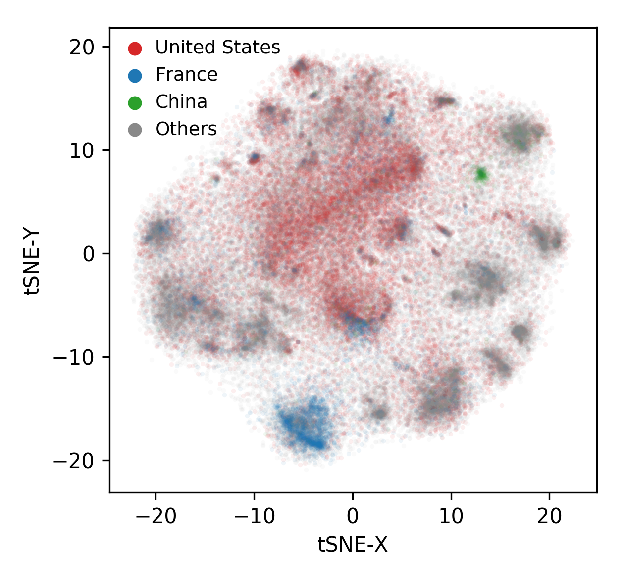
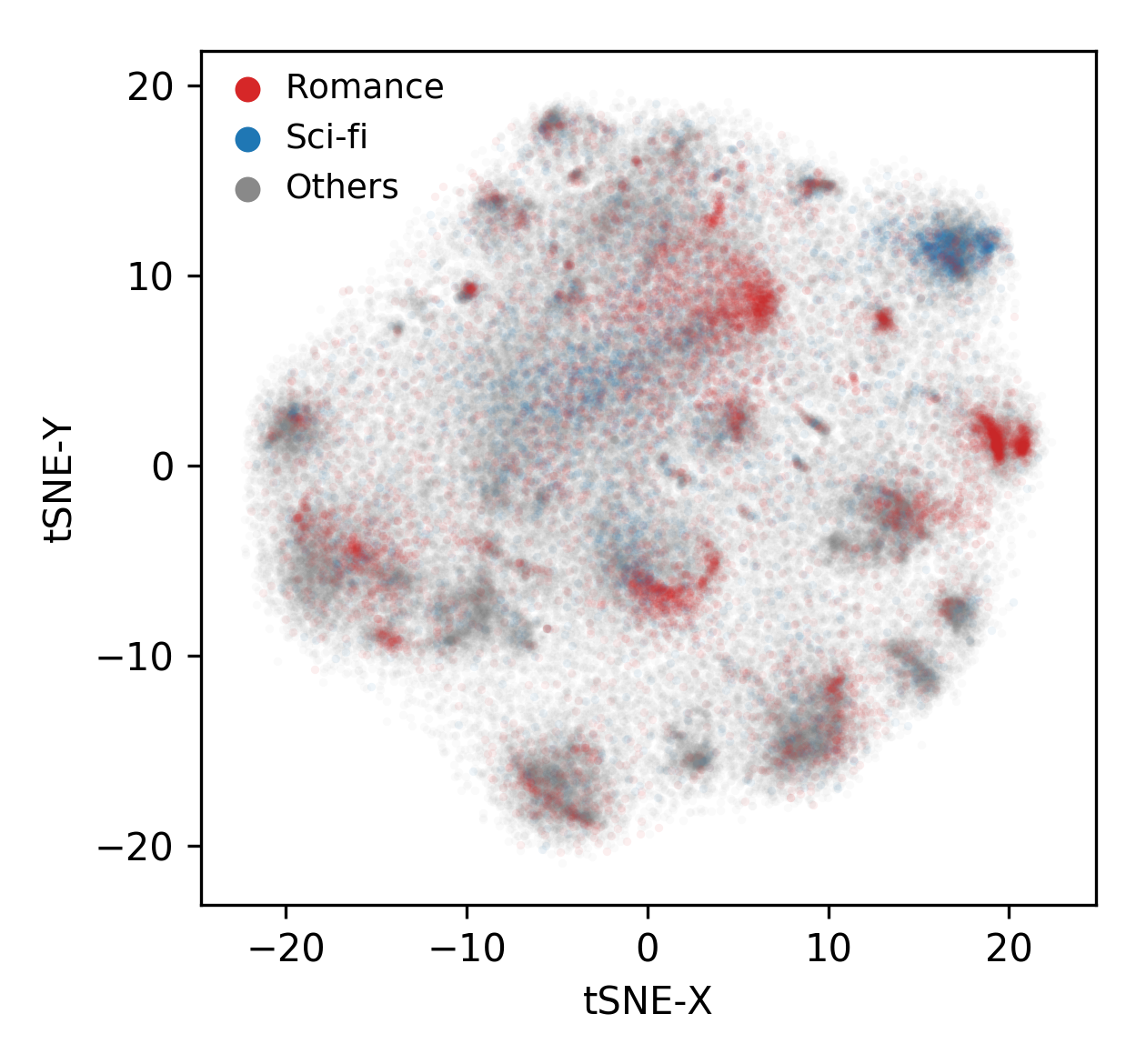
Figure 7 presents a visual example to show how row vectors capture semantic correlations between database tables. We use t-SNE [58] to project embedded vectors of actor names from their original 100-dimensional space into two-dimensional space for plotting. The t-SNE algorithm finds low dimensional embeddings of high dimensional spaces that attempts to maintain the distance between points: points that are close together in the two-dimensional space are close together in the high dimensional space as well, and points that are far apart in the low dimensional space are far apart in the high dimensional space as well.

As shown, various semantic groups (e.g., Chinese actors, sci-fi movie actors) are clustered together (and are thus also close together in the original high-dimensional space), even when these semantic relationships span multiple tables. Intuitively, this provides helpful signals to estimate query latency given similar predicates: as many of the clusters in Figure 7 are linearly separable, their boundaries can be learned by machine learning algorithms. In other words, since predicates with similar semantic values (e.g., two American actors) are likely to have similar correlations (e.g., be in American films), representing the semantic value of a query predicate allows the value network to recognize similar predicates as similar. In Section 6.4.1, we find that row vectors consistently improves Neo’s performance compared to other featurizations.

Row vector construction In our implementation, the feature vectors for query predicates are constructed as follows. For every distinct value in the underlying database, we generate vectors which are a concatenation of the following:

1. One-hot encoding of the comparison operators (e.g. equal or not equal to)

2. Number of matched words

3. Column embedding generated by word2vec (100 values, in our experiments)

4. Number of times the given value is seen in the training

The concatenated vectors replace the “1”s or “0”s in the column predicate vector of 1-Hot representation of the query-level information (see Section 3). For columns without a predicate, zeros are added so that the vector remains the same size regardless of the number of predicates.

5.2 Analysis

Here, we analyze the embedding space learned by our row vector approach on the IMDB dataset. We use the below SQL query from the IMDB database to illustrate how learned row vectors can be useful for tasks like cardinality estimation and query optimization.

This query counts the number of movies with genre “romance” and containing the keyword “love”. It spans five tables in the IMDB dataset. As input to word2vec training, we partially denormalized these tables by joining title, keyword_info, keyword and title, movie_info, info_type. It is important to note that, after this denormalization, keywords and genres do not appear in the same row, but keywords-titles as well as titles-genres do appear in separate rows.

⬇ SELECT count(*) FROM title as t, movie_keyword as mk, keyword as k, info_type as it, movie_info as mi WHERE it.id = 3 AND it.id = mi.info_type_id AND mi.movie_id = t.id AND mk.keyword_id = k.id AND mk.movie_id = t.id AND k.keyword ILIKE '%love%' AND mi.info ILIKE '%romance%'

Figure 8: Example query with correlations

Keyword	Genre	Similarity	Cardinality
love	romance	0.24	11128
love	action	0.16	2157
love	horror	0.09	1542
fight	action	0.28	12177
fight	romance	0.21	3592
fight	horror	0.05	1104

Table 2: Similarity vs. Cardinality. In this case, correlated keywords and genres, as shown in the SQL query in Figure 8, also have higher similarity and higher cardinality.

In Table 2, we compare the cosine similarity (higher value indicating higher similarity) between the vectors for keywords and genres to their true cardinalities in the dataset. As shown, highly correlated keywords and genres (e.g., “love” and “romance”) have higher cardinalities. As a result, this embedding provides a representative feature that can somewhat substitute a precise cardinality estimation: a model built using these vectors as input can learn to understand the correlations within the underlying table.

PostgreSQL, with its uniformity and independence assumptions, always estimates the cardinalities for the final joined result to be close to 1, and therefore prefers to use nested loop joins for this query. In reality, the real cardinalities vary wildly, as shown in Table 2. For this query, Neo decided to use hash joins instead of nested loop joins, and as a result, was able to execute this query $60\%$ faster than PostgreSQL.

This simple example provides a clear indication that row vector embeddings can capture meaningful relationships in the data beyond histograms and one-hot encodings. This, in turn, provides Neo with useful information in the presence of highly correlated columns and values. An additional advantage of our row embedding approach is that, by learning semantic relationships in a given database, Neo can gain useful information even about column predicates that it has never seen before in its training set (e.g., infer similar cardinality using similar correlation between two attributes).

While we can observe useful correlations in the row vectors built for the IMDB dataset, language models like word2vec are notoriously difficult to interpret [45]. To the best of our knowledge, there are no formal methods to ensure that a word2vec model – on either natural language or database rows – will always produce helpful features. Developing such formal analysis is an active area of research in machine learning [37, 31]. Thus, while we have no evidence that our row vector embedding technique will work on every imaginable database, we argue that our analysis on the IMDB database (a database with significant correlations / violations of uniformity assumptions) provides early evidence that row vectors may also be useful in other similar applications with semantically rich datasets. We plan to pursue this as part of our future work.

6 Experiments

We evaluated Neo’s performance using both synthetic and real-world datasets to answer the following questions: (1) how does the performance of Neo compare to commercial, high-quality optimizers, (2) how well does the optimizer generalize to new queries, (3) how long is the optimizer execution and training time, (4) how do the different encoding strategies impact the prediction quality, (5) how do other parameters (e.g., search time or loss function) impact the overall performance, and finally, (6) how robust is Neo to estimation errors.

6.1 Setup

We evaluate Neo across a number of different database systems, using three different benchmarks:

1. JOB: the join order benchmark [25], with a set of queries over the Internet Movie Data Base (IMDB) consisting of complex predicates, designed to test query optimizers.

2. TPC-H: the standard TPC-H benchmark [46], using a scale factor of 10.

3. Corp: a 2TB dataset together with 8,000 unique queries from an internal dashboard application, provided by a large corporation (on the condition of anonymity).

Unless otherwise stated, all experiments are conducted by randomly placing 80% of the available queries into a training set, and using the other 20% of the available queries as a testing set. In the case of TPC-H, we generated 80 training and 20 test queries based on the benchmark query templates without reusing templates between training and test queries.

We present results as the median performance from fifty randomly initialized neural networks. The Adam [19] optimizer is used for network training, as well as layer normalization [3] to stabilize neural network training. The “leaky” variant of rectified linear units [14] are used as activation functions. We use a search time cutoff of 250ms. The network architecture follows Figure 5, except the size of the plan-level encoding is dependent on the featurization chosen (e.g. 1-Hot or Histogram).

6.2 Overall Performance

To evaluate Neo’s overall performance, we compared the mean execution time of the query plans generated by Neo on two open-source (PostgreSQL 11, SQLite 3.27.1), and two commercial (Oracle 12c, Microsoft SQL Server 2017 for Linux) database systems, with the execution time of the plans generated by each system’s native optimizer, for each of our three workloads. Due to the license terms [47] of Microsoft SQL Server and Oracle, we can only show performance in relative terms.

For initial experience collection for Neo, we always used the PostgreSQL optimizer as the expert. That is, for every query in the training set, we used the PostgreSQL optimizer to generate an initial query plan. We then measured the execution time of this plan on the target execution engine (e.g., MS SQL Server) by forcing the target system, through query hints, to obey the proposed query plan. Next, we directly begin training: Neo encodes the execution plan for each query in the training set, these plans are executed on the native system, and the encoded vectors along with the resulting run times are added to Neo’s experience.

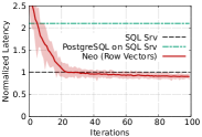
Figure 9 shows the relative performance of Neo after 100 training iterations on each test workload, using the R-Vector encoding over the holdout dataset (lower is better). For example, with PostgreSQL and the JOB workload, Neo produces queries that take only 60% of average execution time than the ones created by the original PostgreSQL optimizer. Since the PostgreSQL optimizer is used to gather initial expertise for Neo, this demonstrates Neo’s ability to improve upon an existing open-source optimizer.

Moreover, for MS SQL Server and the JOB and Corp workloads, the query plans produced by Neo are also 10% faster than the plans created by the commercial optimizers on their native platforms. Importantly, both commercial optimizers, which include a multi-phase search procedure and a dynamically-tuned cost model with hundreds of inputs  [42, 13], are expected to be substantially more advanced than PostgreSQL’s optimizer. Yet, by bootstrapping only with PostgreSQL’s optimizer, Neo is able to eventually outperform or match the performance of these commercial optimizers on their own platforms. Note that the faster execution times are solely based on better query plans without run-time modifications of the system. The only exception where Neo does not outperform the two commercial systems is for the TPC-H workload. We suspect that both MS SQL Server and Oracle were overtuned towards TPC-H, as it is one of the most common benchmarks.

Figure 9: Relative query performance to plans created by the native optimizer (lower is better) for different workloads

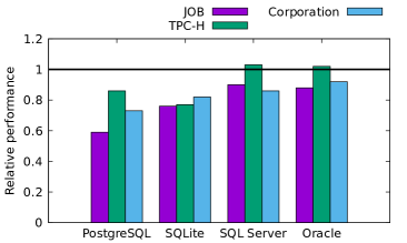
Overall, this experiment demonstrates that Neo is able to create plans, which are as good as, and sometimes even better than, open-source optimizers and their significantly superior commercial counterparts. However, Figure 9 only compares the median performance of Neo after the 100th training episode. This naturally raises the following questions: (1) how does the performance compare with a fewer number of training episodes and how long does it take to train the model to a sufficient quality (answered in the next subsection), and (2) how robust is the optimizer to various imputations (answered in Section 6.4).

6.3 Training Time

To analyze the convergence time, we measured the performance after every training iteration, for a total of 100 complete iterations. We first report the learning curves in training intervals to make the different systems comparable (e.g., a training episode with MS SQL Server might run much faster than PostgreSQL). Afterwards, we report the wall-clock time to train the models on the different systems. Finally, we answer the question of how much our bootstrapping method helped with the training time.

6.3.1 Learning Curves

	PostgreSQL	SQLite	MS SQL Server	Oracle
JOB
TPC-H
Corp

Figure 10: Learning curves with variance. Shaded area spans minimum to maximum across fifty runs with different random seeds. For a plot with all four featurization techniques, please visit: http://rm.cab/l/lc.pdf

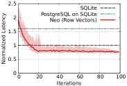
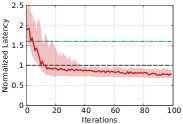
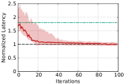
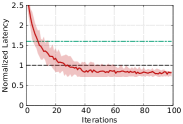
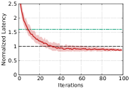
We measured the relative performance of Neo on our entire test suite with respect to the native optimizer (i.e., a performance of $1$ is equivalent to the engine’s optimizer), for every episode (a full pass over the set of training queries, i.e., retraining the network from the experience, choosing a plan for each training query, executing that plan, and adding the result to Neo’s experience) of the 100 complete training episodes of the optimizer. We plot the median value as a solid line, and the minimum and maximum values using the shaded region. For all DBMSes except for PostgreSQL, we additionally plot the relative performance of the plans generated by the PostgreSQL optimizer when executed on the target engine.

Convergence Each figure demonstrates a similar behavior: after the first training iteration, Neo’s performance is poor (e.g., nearly 2.5 times worse than the native optimizer). Then, for several iterations, the performance of Neo sharply improves, until it levels off (converges). We analyze the convergence time specifically in Section 6.3.2. Here, we note that Neo is able to improve on the PostgreSQL optimizer in as few as 9 training iterations (i.e., the number of training iterations until the median run crosses the line representing PostgreSQL). It is not surprising that matching the performance of a commercial optimizer like MS SQL Server or Oracle requires significantly more training iterations than for SQLite, as commercial systems are much more sophisticated.

Variance The variance between the different training iterations is small for all workloads, except for the TPC-H dataset. We hypothesize that, with uniform data distributions in TPC-H, the R-Vector embedding is not as useful, and thus it takes the model longer to adjust accordingly. This behavior is not present in the other two non-synthetic datasets.

6.3.2 Wall-Clock Time

Figure 11: Training time, in minutes, for Neo to match the performance of PostgreSQL and each native optimizer.

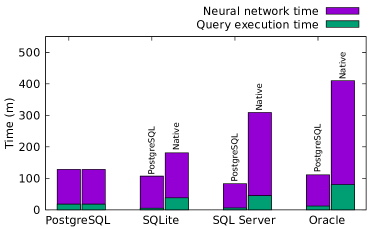
So far, we analyzed how long it took Neo to become competitive in terms of training iterations; next, we analyze the time it takes for Neo to become competitive in terms of wall-clock time (real time). We analyzed how long it took for Neo to learn a policy that was on-par with (1) the query execution plans produced by PostgreSQL, but executed on the target execution engine, and (2) the query plans produced by the native optimizer and executed on the same execution engine. Figure 11 shows the time (in minutes) that it took for Neo to reach these two milestones (the left and right bar charts represent milestone (1) and (2), respectively), split into time spent training the neural network and time spent executing queries. Note that the query execution step is parallelized, executing queries on different nodes simultaneously.

Unsurprisingly, it takes longer for Neo to become competitive with the more advanced, commercial optimizers. However, for every engine, learning a policy that outperforms the PostgreSQL optimizer consistently takes less than two hours. Furthermore, Neo was able to match or exceed the performance of every optimizer within half a day. Note that this time does not include the time for training the query encoding, which in the case of the 1-Hot and Histogram are negligible. However, this takes longer for R-Vector (see Section 6.6).

6.3.3 Is Demonstration Even Necessary?

Since gathering demonstration data introduces additional complexity to the system, it is natural to ask if demonstration data is necessary at all. Is it possible to learn a good policy starting from zero knowledge? While previous work [34] showed that an off-the-shelf deep reinforcement learning technique can learn to find query plans that minimize a cost model without demonstration data, learning a policy based on query latency (i.e., end to end) poses additional difficulties: a bad plan can take hours to execute. Unfortunately, randomly chosen query plans behave exceptionally poorly. Leis et al. showed that randomly sampled join orderings can result in a 100x to 1000x increase in query execution times for JOB queries, compared to a reasonable plan [25], potentially increasing the training time of Neo by a similar factor [35].

We attempted to work around this problem by selecting an ad-hoc query timeout $t$ (e.g., 5 minutes), and terminating query executions when their latencies exceed $t$. However, this technique destroys a good amount of the signal that Neo uses to learn: join patterns resulting in a latency of 7 minutes get the same reward as join patterns resulting in a latency of 1 week, and thus Neo cannot learn that the join patterns in the 7-minute plan are an improvement over the 1-week plan. As a result, even after training for over three weeks, we did not achieve the plan quality that we achieve when bootstrapping the system with the PostgreSQL optimizer.

6.4 Robustness

For all experiments thus far, Neo was always evaluated over the test dataset, never the training dataset. This clearly demonstrates that Neo does generalize to new queries. In this subsection, we study this further by also testing Neo’s performance for the different featurization techniques, over entirely new queries (i.e., queries invented specifically to exhibit novel behavior), and measuring the sensitivity of chosen query plans to cardinality estimation errors.

6.4.1 Featurization

Figure 12: Neo’s performance using each featurization.

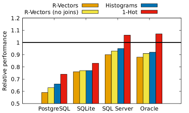
Figure 12 shows the performance of Neo across all four DBMSes for the JOB dataset, varying the featurization used. Here, we examine both the regular R-Vector encoding and a variant of it built without any joins for denormalization (see Section 5). As expected, the 1-Hot encoding consistently performs the worst, as the 1-Hot encoding contains no information about predicate cardinality. The Histogram encoding, while making naive uniformity assumptions, provides enough information about predicate cardinality to improve Neo’s performance. In each case, the R-Vector encoding variants produce the best overall performance, with the “no joins” variant lagging slightly behind. This is because the R-Vector encoding contains significantly more semantic information about the underlying database than the naive histograms (see Section 5). The improved performance of R-Vector compared to the other encoding techniques demonstrates the benefits of tailoring the feature representation used to the underlying data.

6.4.2 On Entirely New Queries

Figure 13: Neo’s performance on entirely new queries (Ext-JOB), full bar height. Neo’s performance after 5 iterations with Ext-JOB queries, solid bar height.

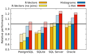
Previous experiments demonstrated Neo’s ability to generalize to queries in a randomly-selected, held-out test set drawn from the same workload as the training set. While this shows that Neo can handle previously-unseen predicates and modifications to join graphs, it does not necessarily demonstrate that Neo will be able to generalize to a completely new query. To test Neo’s behavior on new queries, we created a set of 24 additional queries, which we call Ext-JOB, that are semantically distinct from the original JOB workload (no shared predicates or join graphs).

After Neo had trained for 100 episodes on the JOB queries, we evaluated the relative performance of Neo on the Ext-JOB queries. Figure 13 shows the results: the full height of each bar represents the performance of Neo on the unseen queries relative to every other system. First, we note that with the R-Vector featurization, the execution plans chosen for the entirely-unseen queries in the Ext-JOB dataset still outperformed or matched the native optimizer. Second, the larger gap between the R-Vector featurizations and the Histogram and 1-Hot featurizations demonstrates that row vectors are an effective way of capturing information about query predicates that generalizes to entirely new queries.

Learning new queries Since Neo is able to progressively learn from each query execution, we also evaluated the performance of Neo on the Ext-JOB queries after just 5 additional training episodes. The solid bars in Figure 13 show the results. Once Neo has seen each new query a handful of times, Neo’s performance increases quickly, having learned how to handle the new complexities introduced by the previously-unseen queries. Thus, while the performance of Neo initially degrades when confronted with new queries, Neo quickly adapts its policy to suit these new queries. This showcases the potential for a deep-learning powered query optimizer to keep up with changes in real-world query workloads.

(a) PostgreSQL, $\leq$ 3 joins

(b) PostgreSQL, $>$ 3 joins

(c) True cardinality, $\leq$ 3 joins

(d) True cardinality, $>$ 3 joins

Figure 14: Robustness to cardinality estimation errors

6.4.3 Cardinality Estimates

The strong relationship between cardinality estimation and query optimization is well-studied [4, 39]. However, query optimizers must take into account that most cardinality estimation methods tend to become significantly less accurate when the number of joins increases [25]. While deep neural networks are generally regraded as black boxes, here we show that Neo is capable of learning when to trust cardinality estimates and when to ignore them.

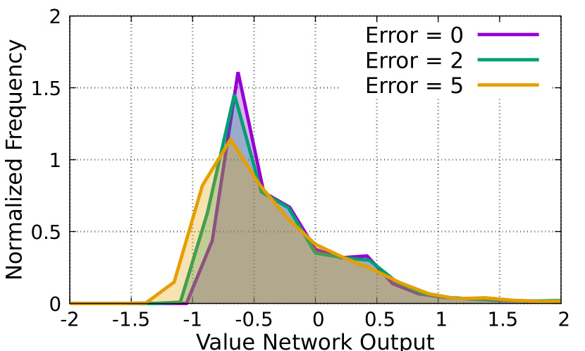
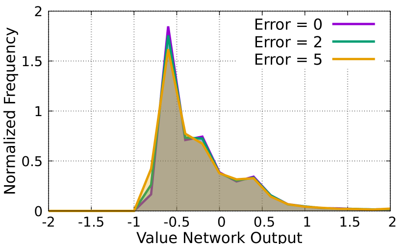
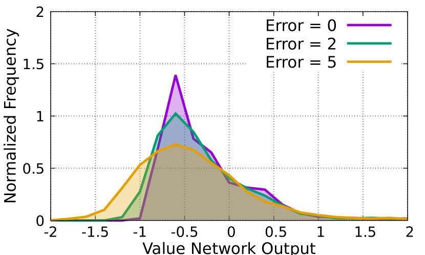
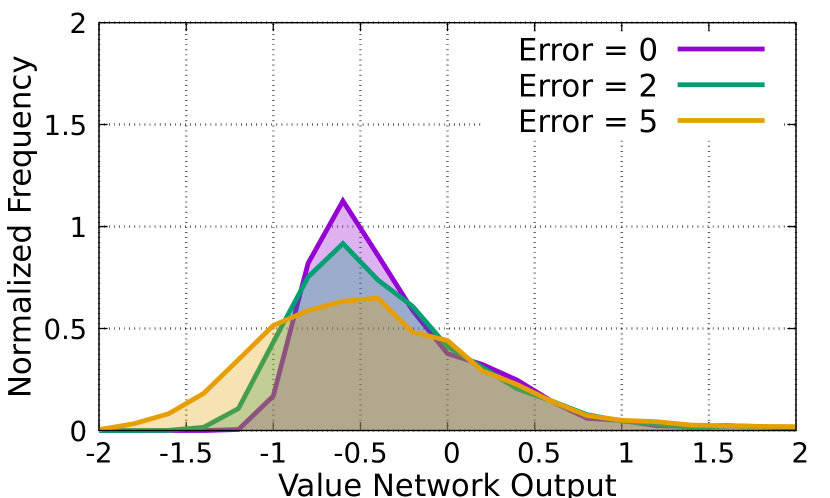
To measure the robustness of Neo to cardinality estimation errors, we trained two Neo models, with an additional feature at each tree node. The first model received the PostgreSQL optimizer’s cardinality estimation, and the second model received the true cardinality. We then plotted a histogram of both model’s outputs across the JOB workload when the number of joins was $\leq 3$ and $>3$, introducing artificial error to the additional features.

For example, Figure 14(a) shows the histogram of value network predictions for all states with at most 3 joins. When the error is increased from zero orders of magnitude to two and five orders of magnitude, the variance of the distribution increases: in other words, when the number of joins is at most 3, Neo learns a model that varies with the PostgreSQL cardinality estimate. However, in Figure 14(b), we see that the distribution of network outputs hardly changes at all when the number of joins is greater than 3: in other words, when the number of joins is greater than 3, Neo learns to ignore the PostgreSQL cardinality estimates all together.

On the other hand, Figure 14(c) and Figure 14(d) show that when Neo’s value model is trained with true cardinalities as inputs, Neo learns a model that varies its prediction with the cardinality regardless of the number of joins. In other words, when provided with true cardinalities, Neo learns to rely on the cardinality information irrespective of the number of joins. Thus, we conclude that Neo is able to learn which input features are reliable, even when the reliability of those features varies with the number of joins.

6.4.4 Per Query Performance

Figure 15: Workload cost vs. relative cost for JOB queries between Neo and PostgreSQL (lower is better)

Finally, we analyzed the per-query performance of Neo (as opposed to the workload performance). The absolute performance improvement (or regression) in seconds for each query of the JOB workload between the Neo and PostgreSQL plans are shown in Figure 15, in purple. As it can be seen, Neo is able to significantly improve the execution time of many queries up to 40 seconds, but also worsens the execution time of a few of queries e.g., query 24a becomes 8.5 seconds slower.

However, in contrast to a traditional optimizer, in Neo we can easily change the optimization goal. So far, we always aimed to optimize the total workload cost, i.e., the total latency across all queries. However, we can also change the optimization goal to optimize for the relative improvement per query (green bars in Figure 15). This implicitly penalizes changes in the query performance from the baseline (e.g., PostgreSQL). When trained with this cost function, the total workload time is still accelerated (by 289 seconds, as opposed to nearly 500 seconds), and all but one query sees improved performance from the PostgreSQL baseline. Thus, we conclude that Neo responds to different optimization goals, allowing it to be customized for different scenarios and for the user’s needs.

It is possible that Neo’s loss function could be further customized to weigh queries differently depending on their importance to the user, i.e. query priority. It may also be possible to build an optimizer that is directly aware of service-level agreements (SLAs). We leave such investigations to future work.

6.5 Search

Figure 16: Search time vs. performance, grouped by number of joins

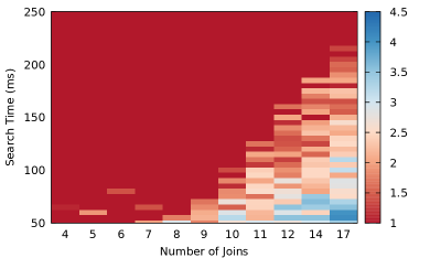
Neo uses the trained value network to search for query plans until a fixed-time cutoff (see Section 4.2). Figure 16 shows how the performance of a query with a particular number of joins (selected randomly from the JOB dataset, executed on PostgreSQL) varies as the search time is changed (previous experiments used a fixed cutoff of 250ms). Note that the x-axis skips some values, e.g. the JOB dataset has no queries with 13 joins. Here, query performance is given relative to the best observed performance. For example, when the number of joins is 10, Neo found the best-observed plan whenever the cutoff time was greater than 120ms. We also tested significantly extending the search time (to 5 minutes), and found that such an extension did not change query performance regardless of the number of joins in the query (up to 17 in the JOB dataset).

The relationship between the number of joins and sensitivity to search time is unsurprising: queries with more joins have a larger search space, and thus require more time to optimize. While 250ms to optimize a query with 17 joins is acceptable in many scenarios, other options [59] may be more desirable when this is not the case.

6.6 Row vector training time

Figure 17: Row vector training time

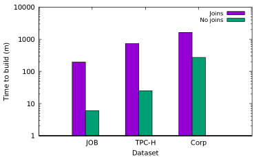
Here, we analyze the time it takes to build the R-Vector representation. Our implementation uses the open source gensim package [48], with no additional optimizations. Figure 17 shows the time it takes to train row vectors on each dataset, for both the “joins” (partially denormalized) and “no joins” (normalized) variants, as described in Section 5. The time to train a row embedding model is proportional to the size of the dataset. For the JOB dataset (approximately 4GB), the “no joins” variant trains in less than 10 minutes, whereas the “no joins” variant for the Corp dataset (approximately 2TB) requires nearly two hours to train. The “joins” (partially denormalized) variant takes significantly longer to train, e.g. three hours (JOB) to a full day (27 hours, Corp).

Building either variant of row vectors may be prohibitive in some cases. However, experimentally we found that, compared to Histogram, the “joins” variant on average resulted in 5% faster query processing times and that the “no joins” variant on average resulted in 3% faster query processing times (e.g., Figure 9). Depending on the multiprocessing level, query arrival rate, etc., row vectors may “pay for themselves” very quickly: for example, the training time for building the “joins” variant on the Corp dataset is “paid for” after 540 hours of query processing, since the row vectors speed up query processing by 5% and require 27 hours to train. As the corporation constantly executes 8 queries simultaneously, this amounts to just three days. The “no joins” variant (improves performance by 3%, takes 217 minutes to train) is “paid for” after just 15 hours.

We do not analyze the behavior of row vectors on a changing database. It is possible that, depending on the database, row vectors quickly become “stale” (the data distribution shifts quickly), or remain relevant for long periods of time (the data distribution shifts slowly). New techniques [11, 62] suggest that retraining word vector models when the underlying data has changed can be done quickly, but we leave investigating these methods to future work.

7 Related work

The relational query optimization problem has been around for more than forty years and is one of the most studied problems in database management systems [52, 8]. Yet, query optimization is still an unsolved problem [29], especially due to the difficulty of accurately estimating cardinalities [25, 26]. IBM DB2’s LEO optimizer was the first to introduce the idea of a query optimizer that learns from its mistakes [54]. In follow-up work, CORDS proactively discovered correlations between any two columns using data samples in advance of query execution [17].

Recent progress in machine learning has led to new ideas for learning-based approaches, especially deep learning [60], to optimizing query run time. For example, recent work  [57, 18] showed how to exploit reinforcement learning for Eddies-style, fine-grained adaptive query processing. More recently, Trummer et al. have proposed the SkinnerDB system, based on the idea of using regret bound as a quality measure while using reinforcement learning for dynamically improving the execution of an individual query in an adaptive query processing system [56]. Ortiz et al. analyzed how state representations affect query optimization when using reinforcement learning [43]. QuickSel offered using query-driven mixture models as an alternative to using histograms and samples for adaptive selectivity learning [44]. Kipf et al. and Liu et al. proposed a deep learning approach to cardinality estimation, specifically designed to capture join-crossing correlations and 0-tuple situations (i.e., empty base table samples) [27, 20]. The closest work to ours is DQ [22], which proposed a learning based approach exclusively for join ordering, and only for a given cost model. The key contribution of our paper over all of these previous approaches is that it provides an end-to-end, continuously learning solution to the database query optimization problem. Our solution does not rely on any hand-crafted cost model or data distribution assumptions.

This paper builds on recent progress from our own team. ReJOIN [34] proposed a deep reinforcement learning approach for join order enumeration [34], which was generalized into a broader vision for designing an end-to-end learning-based query optimizer in [35]. Decima [32] proposed a reinforcement learning-based scheduler, which processes query plans via a graph neural network to learn workload-specific scheduling policies that minimize query latency. SageDB [21] laid out a vision towards building a new type of data processing system which will replace every component of a database system, including the query optimizer, with learned components, thereby gaining the capability to best specialize itself for every use case. This paper is one of the first steps to realizing this overall vision.

8 Conclusions

This paper presents Neo, the first end-to-end learning optimizer that generates highly efficient query execution plans using deep neural networks. Neo iteratively improves its performance through a combination of reinforcement learning and a search strategy. On four database systems and three query datasets, Neo consistently outperforms or matches existing commercial query optimizers (e.g., Oracle’s and Microsoft’s) which have been tuned over decades.

In the future, we plan to investigate various methods for generalizing a learned model to unseen schemas (using e.g. transfer learning [6]). We also intend to further optimize our row vector encoding technique. Finally, we are interested in measuring the performance of Neo when bootstrapping from both more primitive and advanced commercial optimizers. Using a commercial database system as an initial expert might provide substantially faster convergence, or even a better final result (although this would introduce a dependency on a complex, hand-engineered optimizer, defeating a major benefit of Neo). Alternatively, using a simple, Selinger-style [52] optimizer may prove effective, alleviating the need for even the complexities of the PostgreSQL optimizer.

Appendix A neural network model

In this appendix, we present a formal specification of Neo’s neural network model (the value network). An intuitive description is provided in Section 4.

Let the query-level information vector for an execution plan $P$ for a query $Q(P)$ be $V(Q(P))$. Let $F(P)$ be the set of root nodes in the (forest) $P$. We define $L(x)$ and $R(x)$ as the left and right children of a node, respectively. Let $V(x)$ be the vectorized representation of the tree node $x$. We denote all $r\in F(P)$ as the tuple $(r,L(r),R(r))$.

The query-level information $V(Q(P))$ is initially passed through a set of fully connected layers (see Figure 5) of monotonically decreasing size. After the final fully connected layer, the resulting vector $\vec{g}$ is combined with each tree node to form an augmented forest $F^{\prime}(P)$. Intuitively, this augmented forest is created by appending $\vec{g}$ to each tree node. Formally, we define $A(r)$ as the augmenting function for the root of a tree:

$$A(r)=(V(r)\frown\vec{g},A(L(r)),A(R(r)))$$

where $\frown$ is the vector concatenation operator. Then:

$$F^{\prime}(P)=\{A(r)\mid r\in F(P)\}$$

We refer to each entry of an augmented tree node’s vector as a channel. Next, we define tree convolution, an operation that maps a tree with $c_{in}$ channels to a tree with $c_{out}$ channels. The augmented forest is passed through a number of tree convolution layers. Details about tree convolution can be found in [40]. Here, we will provide a mathematical specification. Let a filterbank be a matrix of size $3\times c_{in}\times c_{out}$. We thus define the convolution of a root node $r$ of a tree with $c_{in}$ channels with a filterbank $f$, resulting in an structurally isomorphic tree with $c_{out}$ channels:

$$(r*f)=(V(r)\frown L(r)\frown R(r)\times f,L(r)*f,R(r)*f)$$

We define the convolution of a forest of trees with a filterbank as the convolution of each tree in the forest with the filterbank. The output of the three consecutive tree convolution layers in the value network, with filterbanks $f_{1}$, $f_{2}$, and $f_{3}$, and thus be denoted as:

$$T=((F^{\prime}(P)*f_{1})*f_{2})*f_{3}$$

Let $final_{out}$ be the number of channels in $T$, the output of the consecutive tree convolution layers. Next, we apply a dynamic pooling layer [40]. This layer takes the element-wise maximum of each channel, flattening the forest into a single vector $W$ of size $final_{out}$. Dynamic pooling can be thought of as stacking each tree node’s vectorized representation into a tall matrix of size $n\times final_{out}$, where $n$ is the total number of tree nodes, and then taking the maximum value in each matrix column.

Once produced, $T$ is passed through a final set of fully connected layers, until the final layer of the network produces a singular output. This singular output is used to predict the value of a particular state.

References

- [1] PostgreSQL database, http://www.postgresql.org/.
- [2] T. Anthony, Z. Tian, and D. Barber. Thinking Fast and Slow with Deep Learning and Tree Search. In Advances in Neural Information Processing Systems 30, NIPS ’17, pages 5366–5376, 2017.
- [3] J. L. Ba, J. R. Kiros, and G. E. Hinton. Layer Normalization. arXiv:1607.06450 [cs, stat], July 2016.
- [4] B. Babcock and S. Chaudhuri. Towards a Robust Query Optimizer: A Principled and Practical Approach. In Proceedings of the 2005 ACM SIGMOD International Conference on Management of Data, SIGMOD ’05, pages 119–130, New York, NY, USA, 2005. ACM.
- [5] R. Bellman. A Markovian Decision Process. Indiana University Mathematics Journal, 6(4):679–684, 1957.
- [6] Y. Bengio. Deep Learning of Representations for Unsupervised and Transfer Learning. In Proceedings of ICML Workshop on Unsupervised and Transfer Learning, ICML WUTL ’12, pages 17–36, June 2012.
- [7] R. Bordawekar and O. Shmueli. Using Word Embedding to Enable Semantic Queries in Relational Databases. In Proceedings of the 1st Workshop on Data Management for End-to-End Machine Learning (DEEM), DEEM ’17, pages 5:1–5:4, 2017.
- [8] S. Chaudhuri. An Overview of Query Optimization in Relational Systems. In ACM SIGMOD Symposium on Principles of Database Systems, SIGMOD ’98, pages 34–43, 1998.
- [9] G. V. de la Cruz Jr, Y. Du, and M. E. Taylor. Pre-training Neural Networks with Human Demonstrations for Deep Reinforcement Learning. arXiv:1709.04083 [cs], Sept. 2017.
- [10] R. Dechter and J. Pearl. Generalized Best-first Search Strategies and the Optimality of A*. J. ACM, 32(3):505–536, July 1985.
- [11] M. Faruqui, J. Dodge, S. K. Jauhar, C. Dyer, E. H. Hovy, and N. A. Smith. Retrofitting Word Vectors to Semantic Lexicons. In The 2015 Conference of the North American Chapter of the Association for Computational Linguistics: Human Language Technologies, NAACL ’15, pages 1606–1615, 2015.
- [12] R. C. Fernandez and S. Madden. Termite: A System for Tunneling Through Heterogeneous Data. Preprint, 2019, 2019.
- [13] L. Giakoumakis and C. A. Galindo-Legaria. Testing SQL Server’s Query Optimizer: Challenges, Techniques and Experiences. IEEE Data Eng. Bull., 31:36–43, 2008.
- [14] X. Glorot, A. Bordes, and Y. Bengio. Deep Sparse Rectifier Neural Networks. In G. Gordon, D. Dunson, and M. Dudík, editors, Proceedings of the Fourteenth International Conference on Artificial Intelligence and Statistics, volume 15 of PMLR ’11, pages 315–323, Fort Lauderdale, FL, USA, Apr. 2011. PMLR.
- [15] G. Graefe and W. J. McKenna. The Volcano Optimizer Generator: Extensibility and Efficient Search. In Proceedings of the Ninth International Conference on Data Engineering, ICDE ’93, pages 209–218, Washington, DC, USA, 1993. IEEE Computer Society.
- [16] T. Hester, M. Vecerik, O. Pietquin, M. Lanctot, T. Schaul, B. Piot, D. Horgan, J. Quan, A. Sendonaris, G. Dulac-Arnold, I. Osband, J. Agapiou, J. Z. Leibo, and A. Gruslys. Deep Q-learning from Demonstrations. In Thirty-Second AAAI Conference on Artifical Intelligence, AAAI ’18, New Orleans, Apr. 2017. IEEE.
- [17] I. F. Ilyas, V. Markl, P. Haas, P. Brown, and A. Aboulnaga. CORDS: Automatic Discovery of Correlations and Soft Functional Dependencies. In ACM SIGMOD International Conference on Management of Data, SIGMOD ’04, pages 647–658, 2004.
- [18] T. Kaftan, M. Balazinska, A. Cheung, and J. Gehrke. Cuttlefish: A Lightweight Primitive for Adaptive Query Processing. arXiv preprint, Feb. 2018.
- [19] D. P. Kingma and J. Ba. Adam: A Method for Stochastic Optimization. In 3rd International Conference for Learning Representations, ICLR ’15, San Diego, CA, 2015.
- [20] A. Kipf, T. Kipf, B. Radke, V. Leis, P. Boncz, and A. Kemper. Learned Cardinalities: Estimating Correlated Joins with Deep Learning. In 9th Biennial Conference on Innovative Data Systems Research, CIDR ’19, 2019.
- [21] T. Kraska, M. Alizadeh, A. Beutel, Ed Chi, Ani Kristo, Guillaume Leclerc, Samuel Madden, Hongzi Mao, and Vikram Nathan. SageDB: A Learned Database System. In 9th Biennial Conference on Innovative Data Systems Research, CIDR ’19, 2019.
- [22] S. Krishnan, Z. Yang, K. Goldberg, J. Hellerstein, and I. Stoica. Learning to Optimize Join Queries With Deep Reinforcement Learning. arXiv:1808.03196 [cs], Aug. 2018.
- [23] A. Krizhevsky, I. Sutskever, and G. E. Hinton. ImageNet Classification with Deep Convolutional Neural Networks. In Proceedings of the 25th International Conference on Neural Information Processing Systems - Volume 1, NIPS ’12, pages 1097–1105, USA, 2012. Curran Associates Inc.
- [24] Y. LeCun, Y. Bengio, and G. Hinton. Deep learning. Nature, 521(7553):436–444, May 2015.
- [25] V. Leis, A. Gubichev, A. Mirchev, P. Boncz, A. Kemper, and T. Neumann. How Good Are Query Optimizers, Really? Proc. VLDB Endow., 9(3):204–215, Nov. 2015.
- [26] V. Leis, B. Radke, A. Gubichev, A. Mirchev, P. Boncz, A. Kemper, and T. Neumann. Query optimization through the looking glass, and what we found running the Join Order Benchmark. The VLDB Journal, pages 1–26, Sept. 2017.
- [27] H. Liu, M. Xu, Z. Yu, V. Corvinelli, and C. Zuzarte. Cardinality Estimation Using Neural Networks. In Proceedings of the 25th Annual International Conference on Computer Science and Software Engineering, CASCON ’15, pages 53–59, Riverton, NJ, USA, 2015. IBM Corp.
- [28] W. Liu, Z. Wang, X. Liu, N. Zeng, Y. Liu, and F. E. Alsaadi. A survey of deep neural network architectures and their applications. Neurocomputing, 234:11–26, Apr. 2017.
- [29] G. Lohman. Is Query Optimization a ‘”Solved” Problem? In ACM SIGMOD Blog, ACM Blog ’14, 2014.
- [30] J. Long, E. Shelhamer, and T. Darrell. Fully Convolutional Networks for Semantic Segmentation. In The IEEE Conference on Computer Vision and Pattern Recognition (CVPR), CVPR ’15, June 2015.
- [31] A. L. Maas, R. E. Daly, P. T. Pham, D. Huang, A. Y. Ng, and C. Potts. Learning word vectors for sentiment analysis. In Proceedings of the 49th Annual Meeting of the Association for Computational Linguistics: Human Language Technologies, volume 1 of H:T ’11, pages 142–150. Association for Computational Linguistics, June 2011.
- [32] H. Mao, M. Schwarzkopf, S. B. Venkatakrishnan, Z. Meng, and M. Alizadeh. Learning scheduling algorithms for data processing clusters. arXiv preprint arXiv:1810.01963, 2018.
- [33] G. Marcus. Innateness, AlphaZero, and Artificial Intelligence. arXiv:1801.05667 [cs], Jan. 2018.
- [34] R. Marcus and O. Papaemmanouil. Deep Reinforcement Learning for Join Order Enumeration. In First International Workshop on Exploiting Artificial Intelligence Techniques for Data Management, aiDM ’18, Houston, TX, June 2018.
- [35] R. Marcus and O. Papaemmanouil. Towards a Hands-Free Query Optimizer through Deep Learning. In 9th Biennial Conference on Innovative Data Systems Research, CIDR ’19, 2019.
- [36] T. Mikolov, K. Chen, G. Corrado, and J. Dean. Efficient Estimation of Word Representations in Vector Space. arXiv:1301.3781 [cs], Jan. 2013.
- [37] T. Mikolov, W.-t. Yih, and G. Zweig. Linguistic Regularities in Continuous Space Word Representations. In Proceedings of the 51st Annual Meeting of the Association for Computational Linguistics: Human Language Technologies, HLT ’13, 2013.
- [38] V. Mnih, K. Kavukcuoglu, D. Silver, A. A. Rusu, J. Veness, M. G. Bellemare, A. Graves, M. Riedmiller, A. K. Fidjeland, and G. Ostrovski. Human-level control through deep reinforcement learning. Nature, 518(7540):529–533, 2015.
- [39] G. Moerkotte, T. Neumann, and G. Steidl. Preventing Bad Plans by Bounding the Impact of Cardinality Estimation Errors. Proc. VLDB Endow., 2(1):982–993, Aug. 2009.
- [40] L. Mou, G. Li, L. Zhang, T. Wang, and Z. Jin. Convolutional Neural Networks over Tree Structures for Programming Language Processing. In Proceedings of the Thirtieth AAAI Conference on Artificial Intelligence, AAAI ’16, pages 1287–1293, Phoenix, Arizona, 2016. AAAI Press.
- [41] S. Mudgal, H. Li, T. Rekatsinas, A. Doan, Y. Park, G. Krishnan, R. Deep, E. Arcaute, and V. Raghavendra. Deep Learning for Entity Matching: A Design Space Exploration. In Proceedings of the 2018 International Conference on Management of Data, SIGMOD ’18, pages 19–34, New York, NY, USA, 2018. ACM.
- [42] B. Nevarez. Inside the SQL Server Query Optimizer. Red Gate books, Mar. 2011.
- [43] J. Ortiz, M. Balazinska, J. Gehrke, and S. S. Keerthi. Learning State Representations for Query Optimization with Deep Reinforcement Learning. In 2nd Workshop on Data Managmeent for End-to-End Machine Learning, DEEM ’18, 2018.
- [44] Y. Park, S. Zhong, and B. Mozafari. QuickSel: Quick Selectivity Learning with Mixture Models. arXiv:1812.10568 [cs], Dec. 2018.
- [45] M. Peters, M. Neumann, M. Iyyer, M. Gardner, C. Clark, K. Lee, and L. Zettlemoyer. Deep Contextualized Word Representations. In Proceedings of the 2018 Conference of the North American Chapter of the Association for Computational Linguistics: Human Language Technologies, Volume 1 (Long Papers), NAACL ’18, pages 2227–2237, New Orleans, Louisiana, 2018. Association for Computational Linguistics.
- [46] M. Poess and C. Floyd. New TPC Benchmarks for Decision Support and Web Commerce. SIGMOD Records, 29(4):64–71, Dec. 2000.
- [47] A. G. Read. DeWitt clauses: Can we protect purchasers without hurting Microsoft. Rev. Litig., 25:387, 2006.
- [48] R. Řehůřek and P. Sojka. Software Framework for Topic Modelling with Large Corpora. In Proceedings of the LREC 2010 Workshop on New Challenges for NLP Frameworks, LREC ’10, pages 45–50. ELRA, May 2010.
- [49] S. Schaal. Learning from Demonstration. In Proceedings of the 9th International Conference on Neural Information Processing Systems, NIPS’96, pages 1040–1046, Cambridge, MA, USA, 1996. MIT Press.
- [50] M. Schaarschmidt, A. Kuhnle, B. Ellis, K. Fricke, F. Gessert, and E. Yoneki. LIFT: Reinforcement Learning in Computer Systems by Learning From Demonstrations. arXiv:1808.07903 [cs, stat], Aug. 2018.
- [51] J. Schmidhuber. Deep learning in neural networks: An overview. Neural Networks, 61:85–117, Jan. 2015.
- [52] P. G. Selinger, M. M. Astrahan, D. D. Chamberlin, R. A. Lorie, and T. G. Price. Access Path Selection in a Relational Database Management System. In J. Mylopolous and M. Brodie, editors, SIGMOD ’89, SIGMOD ’89, pages 511–522, San Francisco (CA), 1989. Morgan Kaufmann.
- [53] D. Silver, A. Huang, C. J. Maddison, A. Guez, L. Sifre, G. van den Driessche, J. Schrittwieser, I. Antonoglou, V. Panneershelvam, M. Lanctot, S. Dieleman, D. Grewe, J. Nham, N. Kalchbrenner, I. Sutskever, T. Lillicrap, M. Leach, K. Kavukcuoglu, T. Graepel, and D. Hassabis. Mastering the game of Go with deep neural networks and tree search. Nature, 529(7587):484–489, Jan. 2016.
- [54] M. Stillger, G. M. Lohman, V. Markl, and M. Kandil. LEO - DB2’s LEarning Optimizer. In Proceedings of the 27th International Conference on Very Large Data Bases, VLDB ’01, pages 19–28, San Francisco, CA, USA, 2001. Morgan Kaufmann Publishers Inc.
- [55] N. Tran, A. Lamb, L. Shrinivas, S. Bodagala, and J. Dave. The Vertica Query Optimizer: The case for specialized query optimizers. In 2014 IEEE 30th International Conference on Data Engineering, ICDE ’14, pages 1108–1119, Mar. 2014.
- [56] I. Trummer, S. Moseley, D. Maram, S. Jo, and J. Antonakakis. SkinnerDB: Regret-bounded Query Evaluation via Reinforcement Learning. Proc. VLDB Endow., 11(12):2074–2077, Aug. 2018.
- [57] K. Tzoumas, T. Sellis, and C. Jensen. A Reinforcement Learning Approach for Adaptive Query Processing. Technical Report, 08, June 2008.
- [58] L. van der Maaten and G. Hinton. Visualizing Data using t-SNE. Journal of Machine Learning Research, 9(Nov):2579–2605, 2008.
- [59] F. Waas and A. Pellenkoft. Join Order Selection (Good Enough Is Easy). In Advances in Databases, BNCD ’00, pages 51–67. Springer, Berlin, Heidelberg, July 2000.
- [60] W. Wang, M. Zhang, G. Chen, H. V. Jagadish, B. C. Ooi, and K.-L. Tan. Database Meets Deep Learning: Challenges and Opportunities. SIGMOD Rec., 45(2):17–22, Sept. 2016.
- [61] C. J. Watkins and P. Dayan. Q-learning. Machine learning, 8(3-4):279–292, 1992.
- [62] L. Yu, J. Wang, K. R. Lai, and X. Zhang. Refining Word Embeddings Using Intensity Scores for Sentiment Analysis. IEEE/ACM Transactions on Audio, Speech, and Language Processing, 26(3):671–681, Mar. 2018.
- [63] J.-Y. Zhu, R. Zhang, D. Pathak, T. Darrell, A. A. Efros, O. Wang, and E. Shechtman. Toward Multimodal Image-to-Image Translation. In I. Guyon, U. V. Luxburg, S. Bengio, H. Wallach, R. Fergus, S. Vishwanathan, and R. Garnett, editors, Advances in Neural Information Processing Systems, NIPS ’17, pages 465–476. Curran Associates, Inc., 2017.
- [64] S. Zilberstein. Using Anytime Algorithms in Intelligent Systems. AI Magazine, 17(3):73–73, Mar. 1996.