A unified Eulerian framework for multimaterial continuum mechanics

Haran Jackson hj305@cam.ac.uk Nikos Nikiforakis Cavendish Laboratory, JJ Thomson Ave, Cambridge, UK, CB3 0HE
Abstract

A framework for simulating the interactions between multiple different continua is presented. Each constituent material is governed by the same set of equations, differing only in terms of their equations of state and strain dissipation functions. The interfaces between any combination of fluids, solids, and vacuum are handled by a new Riemann Ghost Fluid Method, which is agnostic to the type of material on either side (depending only on the desired boundary conditions).

The Godunov-Peshkov-Romenski (GPR) model is used for modeling the continua (having recently been used to solve a range of problems involving Newtonian and non-Newtonian fluids, and elastic and elastoplastic solids), and this study represents a novel approach for handling multimaterial problems under this model.

The resulting framework is simple, yet capable of accurately reproducing a wide range of different physical scenarios. It is demonstrated here to accurately reproduce analytical results for known Riemann problems, and to produce expected results in other cases, including some featuring heat conduction across interfaces, and impact-induced deformation and detonation of combustible materials. The framework thus has the potential to streamline development of simulation software for scenarios involving multiple materials and phases of matter, by reducing the number of different systems of equations that require solvers, and cutting down on the amount of theoretical work required to deal with the interfaces between materials.

keywords:
Godunov-Peshkov-Romenski , GPR , Ghost Fluid Method , RGFM , multimaterial
journal: Journal of Computational Physics

1 Background

1.1 Multimaterial Models

This study concerns problems featuring immiscible materials. There are many approaches available to solve these problems, broadly including (but not limited to): Lagrangian and Arbitrary-Lagrangian-Eulerian methods [62, 14], volume of fluid methods [52, 45], diffuse interface methods [61], and level-set methods (including the ghost fluid approach [47, 23]).

Solids models tend to come in Lagrangian form, and often these are combined with ALE forms for the fluid phases, so that the fluid meshes may deform to match the deformation of the solid (see, for example, Pin et al. [51]). These schemes tend to be very accurate, but like all Lagrangian schemes, they fail if the meshes become highly contorted. Thus, adaptive remeshing is often necessary. Some authors have coupled a Lagrangian solid scheme with an Eulerian fluid scheme, but extra care must be taken when applying the boundary conditions to the interface, which corresponds to the intersection of the Eulerian and Lagrangian meshes (see Legay et al. [35] for an implementation using level sets, or Fedkiw [24] for a GFM coupling). Some authors, such as Ryzhakov et al. [58], have found success in using the common Lagrangian formulations for the solid, and a reformulated Lagrangian model for the fluid, implementing the necessary adaptive remeshing. Yet another option is to model both the fluid and the solid in an Eulerian framework, although this now necessitates a level set method or volume of fluid method [29] to track the interfaces. Also, these methods are more prone to losing small-scale geometric features of the media, unless methods such as AMR are employed to combat this [30].

Gavrilyuk, Favrie, et al have presented thermodynamically consistent schemes where solid-fluid interfaces are modeled with the diffuse interface method, with transverse velocities found using a ghost fluid method [21]. The fluid is governed by the compressible Euler equations, and the solid by a conservative hyperelastic model. This was later extended to encompass solids conforming to the visco-plastic model of Maxwell type materials [20], and later still to an arbitrary number of interacting hyperelastic solids and fluids governed by the compressible Euler equations [44].

In a recently submitted paper, Michael and Nikiforakis [41] (building on the work of Schoch et al. [63]) couple various Eulerian models of reactive and inert fluids and solids by use of a Riemann Ghost Fluid Method, with the ghost states calculated using specialised mixed-material Riemann solvers for each interaction (see Section 1.3). Whilst these techniques do not suffer from the mesh contortion issues inherent in Lagrangian formulations of continuum mechanics, a fair amount of theoretical work needs to be done to derive analytical relations describing the interactions between every pair of models used.

If it were possible to describe all phases with the same Eulerian model, this method could be used, with only one type of Riemann solver needed to cope with any multiphase problem posed. The GPR model represents such an opportunity. As will be seen, the model also includes terms for heat conduction, which do not appear in the basic formulations of many of the common models used in multiphase systems (e.g. the Euler equations, or the Godunov-Romenski equations of solid mechanics). Heat conduction is often ignored in multiphase modeling, but such a framework based on the GPR model would almost unavoidably include it.

At present, there is no way of dealing with material interfaces in the GPR model, however. In this study, a modification of Barton’s [2] application of Sambasivan and Udaykumar’s Riemann Ghost Fluid Method [59, 60] is devised for the GPR model, enabling the simulation of material interfaces. This new method is tested on a variety of interface problems.

It is interesting to note that de Brauer et al [13, 10] have presented a method for multimaterial modelling of a similar system (including the distortion tensor of the GPR model, but excluding the heat conduction terms). This method is based on level sets, similar to the method presented in this paper. It should be noted, however, that de Brauer et al do not apply their method to the modelling of viscous flows.

The following two subsections outline the theory behind the GPR model and ghost fluid methods. In Section 2 we explore the eigenstructure of the GPR model, and use it to derive a Riemann solver for the Riemann problem at the interfaces between different materials, which is able to incorporate the boundary conditions that we wish to use. Section 3 presents results of fluid-fluid, solid-solid, fluid-solid, and solid-vacuum problems, including some multidimensional cases, and some incorporating heat conduction across the interfaces. Conclusions are drawn in section 4, along with discussion of potential limitations to the method presented here, and ideas for further avenues of enquiry.

1.2 The Model of Godunov, Peshkov and Romenski

The GPR model takes the following form (see [49, 16, 9, 48]):

ρt+(ρvk)xk𝜌𝑡𝜌subscript𝑣𝑘subscript𝑥𝑘\displaystyle\frac{\partial\rho}{\partial t}+\frac{\partial\left(\rho v_{k}\right)}{\partial x_{k}} =0absent0\displaystyle=0 (1a)
(ρvi)t+(ρvivk+pδikσik)xk𝜌subscript𝑣𝑖𝑡𝜌subscript𝑣𝑖subscript𝑣𝑘𝑝subscript𝛿𝑖𝑘subscript𝜎𝑖𝑘subscript𝑥𝑘\displaystyle\frac{\partial\left(\rho v_{i}\right)}{\partial t}+\frac{\partial(\rho v_{i}v_{k}+p\delta_{ik}-\sigma_{ik})}{\partial x_{k}} =0absent0\displaystyle=0 (1b)
Aijt+(Aikvk)xj+vk(AijxkAikxj)subscript𝐴𝑖𝑗𝑡subscript𝐴𝑖𝑘subscript𝑣𝑘subscript𝑥𝑗subscript𝑣𝑘subscript𝐴𝑖𝑗subscript𝑥𝑘subscript𝐴𝑖𝑘subscript𝑥𝑗\displaystyle\frac{\partial A_{ij}}{\partial t}+\frac{\partial\left(A_{ik}v_{k}\right)}{\partial x_{j}}+v_{k}\left(\frac{\partial A_{ij}}{\partial x_{k}}-\frac{\partial A_{ik}}{\partial x_{j}}\right) =ψijθ1absentsubscript𝜓𝑖𝑗subscript𝜃1\displaystyle=-\frac{\psi_{ij}}{\theta_{1}} (1c)
(ρJi)t+(ρJivk+Tδik)xk𝜌subscript𝐽𝑖𝑡𝜌subscript𝐽𝑖subscript𝑣𝑘𝑇subscript𝛿𝑖𝑘subscript𝑥𝑘\displaystyle\frac{\partial\left(\rho J_{i}\right)}{\partial t}+\frac{\partial\left(\rho J_{i}v_{k}+T\delta_{ik}\right)}{\partial x_{k}} =ρHiθ2absent𝜌subscript𝐻𝑖subscript𝜃2\displaystyle=-\frac{\rho H_{i}}{\theta_{2}} (1d)
(ρE)t+(ρEvk+(pδikσik)vi+qk)xk𝜌𝐸𝑡𝜌𝐸subscript𝑣𝑘𝑝subscript𝛿𝑖𝑘subscript𝜎𝑖𝑘subscript𝑣𝑖subscript𝑞𝑘subscript𝑥𝑘\displaystyle\frac{\partial\left(\rho E\right)}{\partial t}+\frac{\partial\left(\rho Ev_{k}+\left(p\delta_{ik}-\sigma_{ik}\right)v_{i}+q_{k}\right)}{\partial x_{k}} =0absent0\displaystyle=0 (1e)

where ρ𝜌\rho is density, 𝐯𝐯\mathbf{v} is velocity, δ𝛿\delta is the Kronecker delta, p𝑝p is pressure, σ𝜎\sigma is the sheer stress tensor, A𝐴A is the distortion tensor, 𝐉𝐉\mathbf{J} is the thermal impulse vector, T𝑇T is temperature, E𝐸E is total energy, and 𝐪𝐪\mathbf{q} is heat flux. ψ=EA𝜓𝐸𝐴\psi=\frac{\partial E}{\partial A} and 𝑯=E𝑱𝑯𝐸𝑱\boldsymbol{H}=\frac{\partial E}{\partial\boldsymbol{J}}, and θ1subscript𝜃1\theta_{1} and θ2subscript𝜃2\theta_{2} are positive functions (given below for the problems at hand). Additionally, we have:

{p=ρ2Eρ|s,Aσ=ρATEA|ρ,sT=Es|ρ,A𝒒=TE𝑱cases𝑝evaluated-atsuperscript𝜌2𝐸𝜌𝑠𝐴𝜎evaluated-at𝜌superscript𝐴𝑇𝐸𝐴𝜌𝑠𝑇evaluated-at𝐸𝑠𝜌𝐴𝒒𝑇𝐸𝑱\begin{cases}p=\rho^{2}\left.\frac{\partial E}{\partial\rho}\right|_{s,A}&\sigma=-\rho A^{T}\left.\frac{\partial E}{\partial A}\right|_{\rho,s}\\ T=\left.\frac{\partial E}{\partial s}\right|_{\rho,A}&\boldsymbol{q}=T\frac{\partial E}{\partial\boldsymbol{J}}\end{cases} (2)

where s𝑠s is the entropy of the system.

The GPR model represents the same set of equations as the model of elastoplastic deformation originally proposed by Godunov and Romenski. Peshkov and Romenski first subsequently proposed that these are the equations of motion for an arbitrary continuum - not just a solid. In doing so, they were able to apply the model to fluids too. Note that material elements have not only finite size, but also internal structure (encoded in the distortion), unlike in previous continuum models.

The idea of τ1subscript𝜏1\tau_{1} - the strain dissipation time - has its roots in Frenkel’s “particle settled life time” (see [25]). τ1subscript𝜏1\tau_{1} represents a continuous analogue of Frenkel’s object. It can be thought of as the characteristic time taken for a particle to move by a distance roughly the same as the particle’s size. Thus, the typical time taken for a material element to rearrange with its neighbors is characterized by τ1subscript𝜏1\tau_{1} . As long as a continuum description is appropriate for the material at hand, it is thus that the GPR model seeks to describe all three major phases of matter. For example, we have the following relations:

τ1={elasticsolids0inviscidfluidssubscript𝜏1cases𝑒𝑙𝑎𝑠𝑡𝑖𝑐𝑠𝑜𝑙𝑖𝑑𝑠0𝑖𝑛𝑣𝑖𝑠𝑐𝑖𝑑𝑓𝑙𝑢𝑖𝑑𝑠\tau_{1}=\begin{cases}\infty&elastic\,solids\\ 0&inviscid\,fluids\end{cases} (3)

The equation governing 𝑱𝑱\boldsymbol{J} - and its contribution to the system’s total energy - are derived from Romenski’s model of hyperbolic heat transfer, (see [40, 57]). These concepts were later implemented in [56, 53]. The entropy flux is the derivative of the specific internal energy with respect to 𝑱𝑱\boldsymbol{J}, and it is in this way that 𝐉𝐉\mathbf{J} is defined (as the variable conjugate to the entropy flux). As remarked by Romenski, it is more convenient to evolve 𝑱𝑱\boldsymbol{J} and E𝐸E than 𝐪𝐪\mathbf{q} or the entropy flux, and thus the equations take the form given here. Similarly to τ1subscript𝜏1\tau_{1}, τ2subscript𝜏2\tau_{2} is a relaxation time, characterizing the average speed of relaxation of thermal impulse due to heat exchange between neighboring particles.

E𝐸E must be specified to close the system. The energy contains contributions from the micro-, meso-, and macro-scale:

E=E1(ρ,s)+E2(ρ,s,A,𝑱)+E3(𝒗)𝐸subscript𝐸1𝜌𝑠subscript𝐸2𝜌𝑠𝐴𝑱subscript𝐸3𝒗E=E_{1}\left(\rho,s\right)+E_{2}\left(\rho,s,A,\boldsymbol{J}\right)+E_{3}\left(\boldsymbol{v}\right) (4)

E3subscript𝐸3E_{3} is the usual specific kinetic energy per unit mass:

E3=12𝒗2subscript𝐸312superscriptnorm𝒗2E_{3}=\frac{1}{2}\left\|\boldsymbol{v}\right\|^{2} (5)

E2subscript𝐸2E_{2} takes the quadratic form:

E2=cs(ρ,s)24dev(G)F2+ct(ρ,s)22𝑱2subscript𝐸2subscript𝑐𝑠superscript𝜌𝑠24superscriptsubscriptnormdev𝐺𝐹2subscript𝑐𝑡superscript𝜌𝑠22superscriptnorm𝑱2E_{2}=\frac{c_{s}\left(\rho,s\right)^{2}}{4}\left\|\operatorname{dev}\left(G\right)\right\|_{F}^{2}+\frac{c_{t}\left(\rho,s\right)^{2}}{2}\left\|\boldsymbol{J}\right\|^{2} (6)

where

dev(G)=G13tr(G)Idev𝐺𝐺13tr𝐺𝐼\operatorname{dev}\left(G\right)=G-\frac{1}{3}\operatorname{tr}\left(G\right)I (7)

F\left\|\cdot\right\|_{F} is the Frobenius norm111The Frobenius norm is defined by: XF=i,j|Xij|2subscriptnorm𝑋𝐹subscript𝑖𝑗superscriptsubscript𝑋𝑖𝑗2\left\|X\right\|_{F}=\sqrt{\sum_{i,j}\left|X_{ij}\right|^{2}} and G=ATA𝐺superscript𝐴𝑇𝐴G=A^{T}A is the Gramian matrix of the distortion222G𝐺G is known as the Finger tensor in the solid mechanics community, and dev(G)dev𝐺\operatorname{dev}\left(G\right) is the deviator (trace-free part) of G𝐺G. cssubscript𝑐𝑠c_{s} is the characteristic velocity of transverse perturbations. ctsubscript𝑐𝑡c_{t} is related to the characteristic velocity of propagation of heat waves333Note that [16] denotes this variable by α𝛼\alpha, which is avoided here due to a clash with a parameter of one of the equations of state used.:

ch=ctρTcvsubscript𝑐subscript𝑐𝑡𝜌𝑇subscript𝑐𝑣c_{h}=\frac{c_{t}}{\rho}\sqrt{\frac{T}{c_{v}}} (8)

In previous studies (e.g. [16, 9]), ctsubscript𝑐𝑡c_{t} has been taken to be constant, as it will be in this study.

In this study, E1subscript𝐸1E_{1} is taken to be one of the following forms:

1. The stiffened gas EOS:

E1=p+γpρ(γ1)subscript𝐸1𝑝𝛾subscript𝑝𝜌𝛾1E_{1}=\frac{p+\gamma p_{\infty}}{\rho\left(\gamma-1\right)} (9)

2. The shock Mie-Gruneisen EOS:

E1=pref2(1ρ01ρ)+pprefΓ0ρ0subscript𝐸1subscript𝑝𝑟𝑒𝑓21subscript𝜌01𝜌𝑝subscript𝑝𝑟𝑒𝑓subscriptΓ0subscript𝜌0E_{1}=\frac{p_{ref}}{2}\left(\frac{1}{\rho_{0}}-\frac{1}{\rho}\right)+\frac{p-p_{ref}}{\Gamma_{0}\rho_{0}} (10)

where

pref=c02(1ρ01ρ)(1ρ0s(1ρ01ρ))2subscript𝑝𝑟𝑒𝑓superscriptsubscript𝑐021subscript𝜌01𝜌superscript1subscript𝜌0𝑠1subscript𝜌01𝜌2p_{ref}=\frac{c_{0}^{2}\left(\frac{1}{\rho_{0}}-\frac{1}{\rho}\right)}{\left(\frac{1}{\rho_{0}}-s\left(\frac{1}{\rho_{0}}-\frac{1}{\rho}\right)\right)^{2}} (11)

3. The Godunov-Romenski EOS (see [4]):

E1=pργ+c022α2((ρρ0)α1)((12αγ)(ρρ0)α1)subscript𝐸1𝑝𝜌𝛾superscriptsubscript𝑐022superscript𝛼2superscript𝜌subscript𝜌0𝛼112𝛼𝛾superscript𝜌subscript𝜌0𝛼1E_{1}=\frac{p}{\rho\gamma}+\frac{c_{0}^{2}}{2\alpha^{2}}\left(\left(\frac{\rho}{\rho_{0}}\right)^{\alpha}-1\right)\left(\left(1-\frac{2\alpha}{\gamma}\right)\left(\frac{\rho}{\rho_{0}}\right)^{\alpha}-1\right) (12)

with

cs=b0(ρρ0)βsubscript𝑐𝑠subscript𝑏0superscript𝜌subscript𝜌0𝛽c_{s}=b_{0}\left(\frac{\rho}{\rho_{0}}\right)^{\beta} (13)

4. The JWL EOS:

E1=(Aρ0R1eR1ρ0ρ+Bρ0R2eR2ρ0ρ)+p(AeR1ρ0ρ+BeR2ρ0ρ)ρΓ0subscript𝐸1𝐴subscript𝜌0subscript𝑅1superscript𝑒subscript𝑅1subscript𝜌0𝜌𝐵subscript𝜌0subscript𝑅2superscript𝑒subscript𝑅2subscript𝜌0𝜌𝑝𝐴superscript𝑒subscript𝑅1subscript𝜌0𝜌𝐵superscript𝑒subscript𝑅2subscript𝜌0𝜌𝜌subscriptΓ0E_{1}=\left(\frac{A}{\rho_{0}R_{1}}e^{-\frac{R_{1}\rho_{0}}{\rho}}+\frac{B}{\rho_{0}R_{2}}e^{-\frac{R_{2}\rho_{0}}{\rho}}\right)+\frac{p-\left(Ae^{-\frac{R_{1}\rho_{0}}{\rho}}+Be^{-\frac{R_{2}\rho_{0}}{\rho}}\right)}{\rho\Gamma_{0}} (14)

Tabulated equations of state are common-place in the field (see [11, 36, 50] for a range of use cases). There is no a priori reason why they cannot be used for E1subscript𝐸1E_{1} under the framework presented in this study, in the same manner as other hydrodynamic systems (e.g. see [8, 28]). This is out of scope of this paper, however, and presents an avenue of future research. Note that E1,cs,ctsubscript𝐸1subscript𝑐𝑠subscript𝑐𝑡E_{1},c_{s},c_{t} are permitted to depend upon ρ,p𝜌𝑝\rho,p instead of ρ,s𝜌𝑠\rho,s (as is the case in this study), or indeed ρ,T𝜌𝑇\rho,T if the material requires it (such as materials whose shear modulus depend on temperature).

The following forms are taken:

θ1subscript𝜃1\displaystyle\theta_{1} =τ1cs23|A|53τ1={6μρ0cs2Newtonianfluids6μ1nρ0cs2|1𝝈|1nnpowerlawfluidsτ0(σYdev(σ)F)nelastoplasticsolidsformulae-sequenceabsentsubscript𝜏1superscriptsubscript𝑐𝑠23superscript𝐴53subscript𝜏1cases6𝜇subscript𝜌0superscriptsubscript𝑐𝑠2𝑁𝑒𝑤𝑡𝑜𝑛𝑖𝑎𝑛𝑓𝑙𝑢𝑖𝑑𝑠6superscript𝜇1𝑛subscript𝜌0superscriptsubscript𝑐𝑠2superscript1𝝈1𝑛𝑛𝑝𝑜𝑤𝑒𝑟𝑙𝑎𝑤𝑓𝑙𝑢𝑖𝑑𝑠subscript𝜏0superscriptsubscript𝜎𝑌subscriptnormdev𝜎𝐹𝑛𝑒𝑙𝑎𝑠𝑡𝑜𝑝𝑙𝑎𝑠𝑡𝑖𝑐𝑠𝑜𝑙𝑖𝑑𝑠\displaystyle=\frac{\tau_{1}c_{s}^{2}}{3\left|A\right|^{\frac{5}{3}}}\qquad\tau_{1}=\begin{cases}\frac{6\mu}{\rho_{0}c_{s}^{2}}&Newtonian\thinspace fluids\\ \frac{6\mu^{\frac{1}{n}}}{\rho_{0}c_{s}^{2}}\left|\frac{1}{\boldsymbol{\sigma}}\right|^{\frac{1-n}{n}}&power\thinspace law\thinspace fluids\\ \tau_{0}\left(\frac{\sigma_{Y}}{\left\|\operatorname{dev}\left(\sigma\right)\right\|_{F}}\right)^{n}&elastoplastic\thinspace solids\end{cases} (15a)
θ2subscript𝜃2\displaystyle\theta_{2} =τ2ct2ρT0ρ0Tτ2=ρ0κT0ct2formulae-sequenceabsentsubscript𝜏2superscriptsubscript𝑐𝑡2𝜌subscript𝑇0subscript𝜌0𝑇subscript𝜏2subscript𝜌0𝜅subscript𝑇0superscriptsubscript𝑐𝑡2\displaystyle=\tau_{2}c_{t}^{2}\frac{\rho T_{0}}{\rho_{0}T}\qquad\tau_{2}=\frac{\rho_{0}\kappa}{T_{0}c_{t}^{2}} (15b)

The justification of these choices is that classical Navier–Stokes–Fourier theory is recovered in the stiff limit τ1,τ20subscript𝜏1subscript𝜏20\tau_{1},\tau_{2}\rightarrow 0 (see [16]). The rules for power-law fluids and elastoplastic solids are based on material from [33] and [6], respectively.

Finally, it is straightforward to verify that as a consequence of (2) we have the following relations:

σ𝜎\displaystyle\sigma =ρcs2Gdev(G)absent𝜌superscriptsubscript𝑐𝑠2𝐺dev𝐺\displaystyle=-\rho c_{s}^{2}G\operatorname{dev}\left(G\right) (16a)
𝒒𝒒\displaystyle\boldsymbol{q} =ct2T𝑱absentsuperscriptsubscript𝑐𝑡2𝑇𝑱\displaystyle=c_{t}^{2}T\boldsymbol{J} (16b)

and

ψθ1(τ1)𝜓subscript𝜃1subscript𝜏1\displaystyle-\frac{\psi}{\theta_{1}(\tau_{1})} =3τ1(detA)53Adev(G)absent3subscript𝜏1superscript𝐴53𝐴dev𝐺\displaystyle=-\frac{3}{\tau_{1}}\left(\det A\right)^{\frac{5}{3}}A\operatorname{dev}\left(G\right) (17a)
ρ𝑯θ2(τ2)𝜌𝑯subscript𝜃2subscript𝜏2\displaystyle-\frac{\rho\boldsymbol{H}}{\theta_{2}\left(\tau_{2}\right)} =Tρ0T0τ2𝑱absent𝑇subscript𝜌0subscript𝑇0subscript𝜏2𝑱\displaystyle=-\frac{T\rho_{0}}{T_{0}\tau_{2}}\boldsymbol{J} (17b)

Finally, the following constraint holds (see [49]):

det(A)=ρρ0𝐴𝜌subscript𝜌0\det\left(A\right)=\frac{\rho}{\rho_{0}} (18)

See [33] for an interpretation of the physical meaning of the relaxation times τ1,τ2subscript𝜏1subscript𝜏2\tau_{1},\tau_{2} and thermal impulse vector 𝑱𝑱\boldsymbol{J}.

1.3 Ghost Fluid Methods

Ghost fluid methods, combined with level set methods, are used to model the evolution of interfaces between different materials. They are detailed here, as it is with such a method that this study proposes to model the interfaces between different materials described by the GPR model.

1.3.1 Level Set Methods

Given a scalar function f𝑓f on nsuperscript𝑛\mathbb{R}^{n}, the level set of f𝑓f at level c𝑐c is defined as:

Γc={x:f(x)=c}subscriptΓ𝑐conditional-set𝑥𝑓𝑥𝑐\Gamma_{c}=\left\{x:f\left(x\right)=c\right\} (19)

Given normal direction speed v𝑣v, f𝑓f is advected according to the level set equation [46]:

ft=v|f|𝑓𝑡𝑣𝑓\frac{\partial f}{\partial t}=v\left|\nabla f\right| (20)

The advection of a point in a fluid with velocity v𝑣v can be modeled by taking f=|𝐱𝐱𝟎|𝑓𝐱subscript𝐱0f=\left|\mathbf{x-x_{0}}\right| where 𝐱𝟎subscript𝐱0\mathbf{x_{0}} is the position of the point at time t=0𝑡0t=0, and tracking Γ0subscriptΓ0\Gamma_{0}. (20) is solved by an appropriate numerical method. The numerical methods used in this study are described in Chapter 2. f𝑓f will usually have to be renormalized at every time step, to avoid unwanted distortions such as becoming a multivalued function.

1.3.2 The Original Ghost Fluid Method
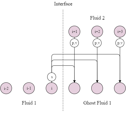
Refer to caption
Figure 1: The Original Ghost Fluid Method

The Original Ghost Fluid Method of Fedkiw et al. [22] (an adaptation of the work of Glimm et al. [26]) is a numerical method for the Euler equations for simulating interfaces between multiple materials. The primitive variables for the Euler equations in 1D are given by 𝑷=(ρvp)T𝑷superscript𝜌𝑣𝑝𝑇\boldsymbol{P}=\left(\begin{array}[]{ccc}\rho&v&p\end{array}\right)^{T}.

Suppose the interface between two fluids is modeled on spatial domain [0,1]01\left[0,1\right], divided into N𝑁N cells with width Δx=1NΔ𝑥1𝑁\Delta x=\frac{1}{N}. Let the time step be ΔtΔ𝑡\Delta t and let 𝑷𝒊𝒏superscriptsubscript𝑷𝒊𝒏\boldsymbol{P_{i}^{n}} be the set of primitive variables in cell i𝑖i at time tn=nΔtsubscript𝑡𝑛𝑛Δ𝑡t_{n}=n\Delta t. Let the level set function f𝑓f have root xnsubscript𝑥𝑛x_{n} where xn[(i+12)Δx,(i+32)Δx]subscript𝑥𝑛𝑖12Δ𝑥𝑖32Δ𝑥x_{n}\in\left[\text{$\left(i+\frac{1}{2}\right)$}\Delta x,\text{$\left(i+\frac{3}{2}\right)$}\Delta x\right]. Thus, at time tnsubscript𝑡𝑛t_{n} the interface lies between the cells with primitive variables 𝑷𝒊𝒏,𝑷𝒊+𝟏𝒏superscriptsubscript𝑷𝒊𝒏superscriptsubscript𝑷𝒊1𝒏\boldsymbol{P_{i}^{n},P_{i+1}^{n}}. Define two sets of primitive variables:

𝑷𝒋(𝟏)={𝑷𝒋𝒏ji(ρ(sin,pjn,γin)vjnpjn)j>isuperscriptsubscript𝑷𝒋1casessuperscriptsubscript𝑷𝒋𝒏𝑗𝑖𝜌superscriptsubscript𝑠𝑖𝑛superscriptsubscript𝑝𝑗𝑛superscriptsubscript𝛾𝑖𝑛superscriptsubscript𝑣𝑗𝑛superscriptsubscript𝑝𝑗𝑛𝑗𝑖\boldsymbol{P_{j}^{\left(1\right)}}=\begin{cases}\boldsymbol{P_{j}^{n}}&j\leq i\\ \left(\begin{array}[]{ccc}\rho\left(s_{i}^{n},p_{j}^{n},\gamma_{i}^{n}\right)&v_{j}^{n}&p_{j}^{n}\end{array}\right)&j>i\end{cases} (21)
𝑷𝒋(𝟐)={𝑷𝒋𝒏ji+1(ρ(si+1n,pjn,γi+1n)vjnpjn)j<i+1superscriptsubscript𝑷𝒋2casessuperscriptsubscript𝑷𝒋𝒏𝑗𝑖1𝜌superscriptsubscript𝑠𝑖1𝑛superscriptsubscript𝑝𝑗𝑛superscriptsubscript𝛾𝑖1𝑛superscriptsubscript𝑣𝑗𝑛superscriptsubscript𝑝𝑗𝑛𝑗𝑖1\boldsymbol{P_{j}^{\left(2\right)}}=\begin{cases}\boldsymbol{P_{j}^{n}}&j\geq i+1\\ \left(\begin{array}[]{ccc}\rho\left(s_{i+1}^{n},p_{j}^{n},\gamma_{i+1}^{n}\right)&v_{j}^{n}&p_{j}^{n}\end{array}\right)&j<i+1\end{cases} (22)

where:

ρ(s,p,γ)=(ps)1γ𝜌𝑠𝑝𝛾superscript𝑝𝑠1𝛾\rho\left(s,p,\gamma\right)=\left(\frac{p}{s}\right)^{\frac{1}{\gamma}} (23)

All cells in 𝑷(𝟏)superscript𝑷1\boldsymbol{P^{\left(1\right)}} to the left of the interface have the same state variables as those of 𝑷𝒏superscript𝑷𝒏\boldsymbol{P^{n}}. All cells to the right have the same pressure and velocity as their counterparts in 𝑷𝒏superscript𝑷𝒏\boldsymbol{P^{n}}, but the same entropy as 𝑷𝒊𝒏superscriptsubscript𝑷𝒊𝒏\boldsymbol{P_{i}^{n}}. This affects their density. The situation is analogous for 𝑷(𝟐)superscript𝑷2\boldsymbol{P^{\left(2\right)}}. This is demonstrated in Figure 1 on page 1.

𝑷(𝟏),𝑷(𝟐)superscript𝑷1superscript𝑷2\boldsymbol{P^{\left(1\right)}},\boldsymbol{P^{\left(2\right)}} are stepped forward by time step ΔtΔ𝑡\Delta t using a standard Eulerian method. f𝑓f is advected using (20), taking the velocity in each cell to be that of 𝑷𝒏superscript𝑷𝒏\boldsymbol{P^{n}}. Now let f(xn+1)=0𝑓subscript𝑥𝑛10f\left(x_{n+1}\right)=0 where xn+1[(k+12)Δx,(k+32)Δx]subscript𝑥𝑛1𝑘12Δ𝑥𝑘32Δ𝑥x_{n+1}\in\left[\left(k+\frac{1}{2}\right)\Delta x,\left(k+\frac{3}{2}\right)\Delta x\right] for some k𝑘k. Define:

𝑷𝒋𝒏+𝟏={𝑷𝒋(𝟏)jk𝑷𝒋(𝟐)j>ksuperscriptsubscript𝑷𝒋𝒏1casessuperscriptsubscript𝑷𝒋1𝑗𝑘superscriptsubscript𝑷𝒋2𝑗𝑘\boldsymbol{P_{j}^{n+1}}=\begin{cases}\boldsymbol{P_{j}^{\left(1\right)}}&j\leq k\\ \boldsymbol{P_{j}^{\left(2\right)}}&j>k\end{cases} (24)

The rationale behind the original GFM is that in most applications, pressure and velocity are continuous across the interface, and thus the ghost cells may take the real pressure and velocity values. Entropy is generally discontinuous at a contact discontinuity, resulting in large truncation errors if a standard finite difference scheme is used to solve the system. Thus, entropy is extrapolated as a constant from the interface boundary cell into the ghost region.
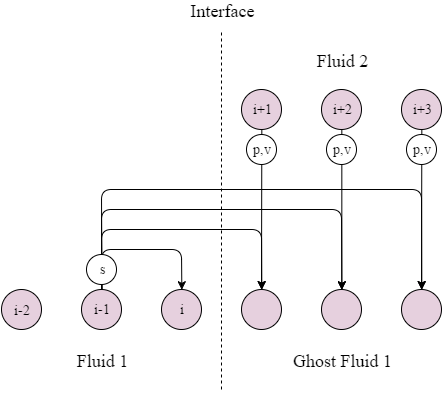
Refer to caption
Figure 2: The Original Ghost Fluid Method, with the isobaric fix

Fedkiw et al. advised to use the isobaric fix technique. This involves setting the entropy of cell i𝑖i, and all cells in the right ghost region, to that of cell i1𝑖1i-1, and setting the entropy of cell i+1𝑖1i+1, and all cells in the left ghost region, to that of cell i+2𝑖2i+2. This is demonstrated in Figure 2 on page 2.

Effectively, the ghost regions behave like they are composed of the same fluid as the regions they extend (as they have the same entropy), facilitating calculation of the next time step, but they have the same pressure and velocity profiles as the real fluids they replace, meaning the boundary conditions at the interface are upheld.
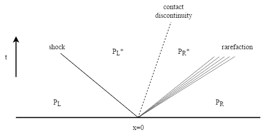
Refer to caption
Figure 3: The qualitative structure of the solution to the Riemann Problem, showing the different possible types of waves

1.3.3 The Riemann Ghost Fluid Method

The Riemann Problem in its general form is the solution of the following initial value problem. Given a set of variables 𝑷𝑷\boldsymbol{P} dependent on space and time, and a hyperbolic set of equations which govern their spatio-temporal evolution, 𝑷(x,t)𝑷𝑥𝑡\boldsymbol{P}\left(x,t\right) is sought for t>0𝑡0t>0, given the initial condition:

𝑷(x,0)={𝑷𝑳x<0𝑷𝑹x>0𝑷𝑥0casessubscript𝑷𝑳𝑥0subscript𝑷𝑹𝑥0\boldsymbol{P}\left(x,0\right)=\begin{cases}\boldsymbol{P_{L}}&x<0\\ \boldsymbol{P_{R}}&x>0\end{cases} (25)

This problem is denoted by RP(𝑷𝑳,𝑷𝑹)𝑅𝑃subscript𝑷𝑳subscript𝑷𝑹RP\left(\boldsymbol{P_{L}},\boldsymbol{P_{R}}\right). Exact solvers exist for the Riemann Problem for various sets of governing equations, such as the Euler equations [65], the equations of non-linear elasticity [5], or the shallow water equations [1], among others. There also exist approximate solvers for general conservative [43, 38] or non-conservative [15] hyperbolic systems of PDEs. The references given here form a very small sample of the work that has been done in this area.

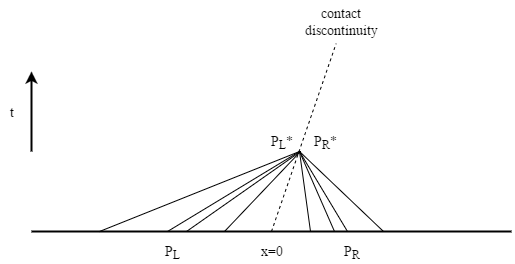
The solution of the Riemann Problem usually takes the form of a set of waves, between which 𝑷𝑷\boldsymbol{P} is constant. The waves can either be a contact discontinuity (across which pressure and velocity are continuous), a shock (across which all variables may be discontinuous), or a rarefaction (along which the variables vary continuously between their values on either side of the wave). The number and form of the waves are determined by the governing equations and the initial conditions. The states of the variables either side of the contact discontinuity in the middle are known as the star states. This qualitative description is depicted in Figure 3 on page 3.

Liu et al. [37] demonstrated that the original GFM fails to resolve strong shocks at material interfaces. This is because the method effectively solves two separate single-fluid Riemann problems. The waves present in these Riemann problems do not necessarily correspond to those in the real Riemann problem across the interface. The Riemann Ghost Fluid Method of Sambasivan et al. [59] aims to rectify this.

Given 𝑷𝒏superscript𝑷𝒏\boldsymbol{P^{n}} and xn[(i+12)Δx,(i+32)Δx]subscript𝑥𝑛𝑖12Δ𝑥𝑖32Δ𝑥x_{n}\in\left[\left(i+\frac{1}{2}\right)\Delta x,\left(i+\frac{3}{2}\right)\Delta x\right], the ghost cells for fluid 1 are populated with the left star state of RP(𝑷𝒊𝟏𝒏,𝑷𝒊+𝟐𝒏)𝑅𝑃superscriptsubscript𝑷𝒊1𝒏superscriptsubscript𝑷𝒊2𝒏RP\left(\boldsymbol{P_{i-1}^{n}},\boldsymbol{P_{i+2}^{n}}\right), and the ghost cells for fluid 2 are populated with the right star state. RP(𝑷𝒊𝟏𝒏,𝑷𝒊+𝟐𝒏)𝑅𝑃superscriptsubscript𝑷𝒊1𝒏superscriptsubscript𝑷𝒊2𝒏RP\left(\boldsymbol{P_{i-1}^{n}},\boldsymbol{P_{i+2}^{n}}\right) is solved rather than RP(𝑷𝒊𝒏,𝑷𝒊+𝟏𝒏)𝑅𝑃superscriptsubscript𝑷𝒊𝒏superscriptsubscript𝑷𝒊1𝒏RP\left(\boldsymbol{P_{i}^{n}},\boldsymbol{P_{i+1}^{n}}\right), as 𝑷𝒊𝒏,𝑷𝒊+𝟏𝒏superscriptsubscript𝑷𝒊𝒏superscriptsubscript𝑷𝒊1𝒏\boldsymbol{P_{i}^{n}},\boldsymbol{P_{i+1}^{n}} often contain errors generated by the fact that they lie on the material interface. 𝑷𝒏+𝟏superscript𝑷𝒏1\boldsymbol{P^{n+1}} is then generated as before from the newly formed 𝑷(𝟏),𝑷(𝟐)superscript𝑷1superscript𝑷2\boldsymbol{P^{\left(1\right)}},\boldsymbol{P^{\left(2\right)}}. This process is demonstrated in Figure 4 on page 4.
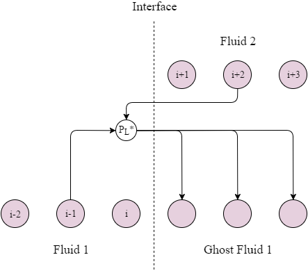
Refer to caption
Figure 4: The Riemann Ghost Fluid Method

1.4 Finite Volume Scheme

The presented system is solved with a finite volume scheme in this study, using a regularized square meshing. Once the values of the ghost cells have been calculated, we require a numerical method to calculate the value of the grid at the next time step. In this study, the finite volume method presented in [32, 33] was used. It is outlined here for completeness.

Note that (1a), (1b), (1c), (1d), (1e) can be written in the following form:

𝑸t+𝑭(𝑸)+𝑩(𝑸)𝑸=𝑺(𝑸)𝑸𝑡bold-∇𝑭𝑸𝑩𝑸𝑸𝑺𝑸\frac{\partial\boldsymbol{Q}}{\partial t}+\boldsymbol{\nabla}\cdot\boldsymbol{F}\left(\boldsymbol{Q}\right)+\boldsymbol{B}\left(\boldsymbol{Q}\right)\cdot\nabla\boldsymbol{Q}=\boldsymbol{S}\left(\boldsymbol{Q}\right) (26)

As described in [64], a method to solve a system such as this is to solve the following subsystems:

𝑸t+𝑭(𝑸)+𝑩(𝑸)𝑸𝑸𝑡bold-∇𝑭𝑸𝑩𝑸𝑸\displaystyle\frac{\partial\boldsymbol{Q}}{\partial t}+\boldsymbol{\nabla}\cdot\boldsymbol{F}\left(\boldsymbol{Q}\right)+\boldsymbol{B}\left(\boldsymbol{Q}\right)\cdot\nabla\boldsymbol{Q} =𝟎absent0\displaystyle=\boldsymbol{0} (27a)
d𝑸dt𝑑𝑸𝑑𝑡\displaystyle\frac{d\boldsymbol{Q}}{dt} =𝑺(𝑸)absent𝑺𝑸\displaystyle=\boldsymbol{S}\left(\boldsymbol{Q}\right) (27b)

Let Hδt,Sδtsuperscript𝐻𝛿𝑡superscript𝑆𝛿𝑡H^{\delta t},S^{\delta t} be the operators that take data 𝑸(x,t)𝑸𝑥𝑡\boldsymbol{Q}\left(x,t\right) to 𝑸(x,t+δt)𝑸𝑥𝑡𝛿𝑡\boldsymbol{Q}\left(x,t+\delta t\right) under systems (27a) and (27b) respectively. A second-order scheme (in time) for solving the full set of PDEs over time step [0,Δt]0Δ𝑡\left[0,\Delta t\right] is obtained by calculating 𝑸𝚫𝒕subscript𝑸𝚫𝒕\boldsymbol{Q_{\Delta t}} using a Strang splitting:

𝑸𝚫𝒕=SΔt2HΔtSΔt2𝑸𝟎subscript𝑸𝚫𝒕superscript𝑆Δ𝑡2superscript𝐻Δ𝑡superscript𝑆Δ𝑡2subscript𝑸0\boldsymbol{Q_{\Delta t}}=S^{\frac{\Delta t}{2}}H^{\Delta t}S^{\frac{\Delta t}{2}}\boldsymbol{Q_{0}} (28)

In this study, the homogeneous subsystem is be solved using a WENO reconstruction of the data, followed by a finite volume update, and the temporal ODEs will be solved with appropriate ODE solvers. The WENO method was chosen due to the arbitrarily high-order spatial reconstructions it is able to produce.

Noting that dρdt=0𝑑𝜌𝑑𝑡0\frac{d\rho}{dt}=0 over the ODE time step, the operator S𝑆S entails solving the following systems:

dAdt𝑑𝐴𝑑𝑡\displaystyle\frac{dA}{dt} =3τ1(detA)53Adev(G)absent3subscript𝜏1superscript𝐴53𝐴dev𝐺\displaystyle=\frac{-3}{\tau_{1}}\left(\det A\right)^{\frac{5}{3}}A\operatorname{dev}\left(G\right) (29a)
d𝑱dt𝑑𝑱𝑑𝑡\displaystyle\frac{d\boldsymbol{J}}{dt} =1τ2Tρ0T0ρ𝑱absent1subscript𝜏2𝑇subscript𝜌0subscript𝑇0𝜌𝑱\displaystyle=-\frac{1}{\tau_{2}}\frac{T\rho_{0}}{T_{0}\rho}\boldsymbol{J} (29b)

These systems are solved separately, and thus he second-order Strang splitting becomes:

𝑸𝚫𝒕=DΔt2TΔt2HΔtTΔt2DΔt2𝑸𝟎subscript𝑸𝚫𝒕superscript𝐷Δ𝑡2superscript𝑇Δ𝑡2superscript𝐻Δ𝑡superscript𝑇Δ𝑡2superscript𝐷Δ𝑡2subscript𝑸0\boldsymbol{Q_{\Delta t}}=D^{\frac{\Delta t}{2}}T^{\frac{\Delta t}{2}}H^{\Delta t}T^{\frac{\Delta t}{2}}D^{\frac{\Delta t}{2}}\boldsymbol{Q_{0}} (30)

where Dδt,Tδtsuperscript𝐷𝛿𝑡superscript𝑇𝛿𝑡D^{\delta t},T^{\delta t} are the operators solving the distortion and thermal impulse ODEs respectively, over time step δt𝛿𝑡\delta t.

The constraint (18) is enforced by rescaling the singular values of the distortion all by the same factor at each timestep, to ensure that detA=ρρ0𝐴𝜌subscript𝜌0\det A=\frac{\rho}{\rho_{0}}.

1.4.1 The Homogeneous System

A WENO reconstruction of the cell-averaged data is performed at the start of the time step (as described in [19]). Focusing on a single cell Cisubscript𝐶𝑖C_{i} at time tnsubscript𝑡𝑛t_{n}, we have 𝒘𝒏(𝒙)=𝒘𝒏pΨp(𝝌(𝒙))superscript𝒘𝒏𝒙subscriptsuperscript𝒘𝒏𝑝subscriptΨ𝑝𝝌𝒙\boldsymbol{w^{n}}\left(\boldsymbol{x}\right)=\boldsymbol{w^{n}}_{p}\Psi_{p}\left(\boldsymbol{\chi}\left(\boldsymbol{x}\right)\right) in Cisubscript𝐶𝑖C_{i} where ΨpsubscriptΨ𝑝\Psi_{p} is a tensor product of basis functions in each of the spatial dimensions. The flux in C𝐶C is approximated by 𝑭(𝒙)𝑭(𝒘p)Ψp(𝝌(𝒙))𝑭𝒙𝑭subscript𝒘𝑝subscriptΨ𝑝𝝌𝒙\boldsymbol{F}\left(\boldsymbol{x}\right)\approx\boldsymbol{F}\left(\boldsymbol{w}_{p}\right)\Psi_{p}\left(\boldsymbol{\chi}\left(\boldsymbol{x}\right)\right). 𝒘psubscript𝒘𝑝\boldsymbol{w}_{p} are stepped forwards half a time step using the update formula:

𝒘𝒑𝒏+𝟏𝟐𝒘𝒑𝒏Δt/2=superscriptsubscript𝒘𝒑𝒏12superscriptsubscript𝒘𝒑𝒏Δ𝑡2absent\displaystyle\frac{\boldsymbol{w_{p}^{n+\frac{1}{2}}}-\boldsymbol{w_{p}^{n}}}{\Delta t/2}= 𝑭(𝒘𝒌𝒏)Ψk(𝝌𝒑)𝑭superscriptsubscript𝒘𝒌𝒏subscriptΨ𝑘subscript𝝌𝒑\displaystyle-\boldsymbol{F}\left(\boldsymbol{w_{k}^{n}}\right)\cdot\nabla\Psi_{k}\left(\boldsymbol{\chi_{p}}\right) (31)
𝑩(𝒘𝒑𝒏)(𝒘𝒌𝒏Ψk(𝝌𝒑))𝑩superscriptsubscript𝒘𝒑𝒏superscriptsubscript𝒘𝒌𝒏subscriptΨ𝑘subscript𝝌𝒑\displaystyle-\boldsymbol{B}\left(\boldsymbol{w_{p}^{n}}\right)\cdot\left(\boldsymbol{w_{k}^{n}}\nabla\Psi_{k}\left(\boldsymbol{\chi_{p}}\right)\right)

i.e.

𝒘𝒑𝒏+𝟏𝟐=𝒘𝒑𝒏Δt2Δx(𝑭(𝒘𝒌𝒏)Ψk(𝝌𝒑)+𝑩(𝒘𝒑𝒏)(𝒘𝒌𝒏Ψk(𝝌𝒑)))superscriptsubscript𝒘𝒑𝒏12superscriptsubscript𝒘𝒑𝒏Δ𝑡2Δ𝑥𝑭superscriptsubscript𝒘𝒌𝒏subscriptΨ𝑘subscript𝝌𝒑𝑩superscriptsubscript𝒘𝒑𝒏superscriptsubscript𝒘𝒌𝒏subscriptΨ𝑘subscript𝝌𝒑\boldsymbol{w_{p}^{n+\frac{1}{2}}}=\boldsymbol{w_{p}^{n}}-\frac{\Delta t}{2\Delta x}\left(\begin{array}[]{c}\boldsymbol{F}\left(\boldsymbol{w_{k}^{n}}\right)\cdot\nabla\Psi_{k}\left(\boldsymbol{\chi_{p}}\right)\\ +\boldsymbol{B}\left(\boldsymbol{w_{p}^{n}}\right)\cdot\left(\boldsymbol{w_{k}^{n}}\nabla\Psi_{k}\left(\boldsymbol{\chi_{p}}\right)\right)\end{array}\right) (32)

where 𝝌𝒑subscript𝝌𝒑\boldsymbol{\chi_{p}} is the node corresponding to ΨpsubscriptΨ𝑝\Psi_{p}.

Integrating (27a) over C𝐶C gives:

𝑸𝒊𝒏+𝟏=𝑸𝒊𝒏Δtn(𝑷𝒊𝒏+𝟏𝟐+𝑫𝒊𝒏+𝟏𝟐)superscriptsubscript𝑸𝒊𝒏1superscriptsubscript𝑸𝒊𝒏Δsubscript𝑡𝑛superscriptsubscript𝑷𝒊𝒏12superscriptsubscript𝑫𝒊𝒏12\boldsymbol{Q_{i}^{n+1}}=\boldsymbol{Q_{i}^{n}}-\Delta t_{n}\left(\boldsymbol{P_{i}^{n+\frac{1}{2}}}+\boldsymbol{D_{i}^{n+\frac{1}{2}}}\right) (33)

where

𝑸𝒊𝒏superscriptsubscript𝑸𝒊𝒏\displaystyle\boldsymbol{Q_{i}^{n}} =1VC𝑸(𝒙,tn)𝑑𝒙absent1𝑉subscript𝐶𝑸𝒙subscript𝑡𝑛differential-d𝒙\displaystyle=\frac{1}{V}\int_{C}\boldsymbol{Q}\left(\boldsymbol{x},t_{n}\right)d\boldsymbol{x} (34a)
𝑷𝒊𝒏+𝟏𝟐superscriptsubscript𝑷𝒊𝒏12\displaystyle\boldsymbol{P_{i}^{n+\frac{1}{2}}} =1VC𝑩(𝑸(𝒙,tn+12))𝑸(𝒙,tn+12)𝑑𝒙absent1𝑉subscript𝐶𝑩𝑸𝒙subscript𝑡𝑛12𝑸𝒙subscript𝑡𝑛12differential-d𝒙\displaystyle=\frac{1}{V}\int_{C}\boldsymbol{B}\left(\boldsymbol{Q}\left(\boldsymbol{x},t_{n+\frac{1}{2}}\right)\right)\cdot\nabla\boldsymbol{Q}\left(\boldsymbol{x},t_{n+\frac{1}{2}}\right)d\boldsymbol{x} (34b)
𝑫𝒊𝒏+𝟏𝟐superscriptsubscript𝑫𝒊𝒏12\displaystyle\boldsymbol{D_{i}^{n+\frac{1}{2}}} =1VC𝓓(𝑸(𝒔,tn+12),𝑸+(𝒔,tn+12))𝑑𝒔absent1𝑉subscriptcontour-integral𝐶𝓓superscript𝑸𝒔subscript𝑡𝑛12superscript𝑸𝒔subscript𝑡𝑛12differential-d𝒔\displaystyle=\frac{1}{V}\oint_{\partial C}\boldsymbol{\mathcal{D}}\left(\boldsymbol{Q^{-}}\left(\boldsymbol{s},t_{n+\frac{1}{2}}\right),\boldsymbol{Q^{+}}\left(\boldsymbol{s},t_{n+\frac{1}{2}}\right)\right)d\boldsymbol{s} (34c)

where V𝑉V is the volume of C𝐶C and 𝑸,𝑸+superscript𝑸superscript𝑸\boldsymbol{Q^{-},Q^{+}} are the interior and exterior extrapolated states at the boundary of C𝐶C, respectively.

Note that (27a) can be rewritten as:

𝑸t+𝑴(𝑸)𝑸=𝟎𝑸𝑡𝑴𝑸𝑸0\frac{\partial\boldsymbol{Q}}{\partial t}+\boldsymbol{M}\left(\boldsymbol{Q}\right)\cdot\nabla\boldsymbol{Q}=\boldsymbol{0} (35)

where 𝑴=𝑭𝑸+𝑩𝑴𝑭𝑸𝑩\boldsymbol{M}=\frac{\partial\boldsymbol{F}}{\partial\boldsymbol{Q}}+\boldsymbol{B}. Let 𝒏𝒏\boldsymbol{n} be the normal to the boundary at point 𝒔C𝒔𝐶\boldsymbol{s}\in\partial C. For the GPR model, M^=𝑴(𝑸(𝒔))𝒏^𝑀𝑴𝑸𝒔𝒏\hat{M}=\boldsymbol{M}\left(\boldsymbol{Q}\left(\boldsymbol{s}\right)\right)\cdot\boldsymbol{n} is a diagonalizable matrix with decomposition M^=R^Λ^R^1^𝑀^𝑅^Λsuperscript^𝑅1\hat{M}=\hat{R}\hat{\Lambda}\hat{R}^{-1} where the columns of R^^𝑅\hat{R} are the right eigenvectors and Λ^^Λ\hat{\Lambda} is the diagonal matrix of eigenvalues. Define also 𝑭^=𝑭𝒏bold-^𝑭𝑭𝒏\boldsymbol{\hat{F}}=\boldsymbol{F}\cdot\boldsymbol{n} and B^=𝑩𝒏^𝐵𝑩𝒏\hat{B}=\boldsymbol{B}\cdot\boldsymbol{n}. Using these definitions, the interface terms arising in the FV formula have the following form:

𝓓(𝑸,𝑸+)𝓓superscript𝑸superscript𝑸\displaystyle\boldsymbol{\mathcal{D}}\left(\boldsymbol{Q^{-}},\boldsymbol{Q^{+}}\right) =12(𝑭^(𝑸+)+𝑭^(𝑸))absent12bold-^𝑭superscript𝑸bold-^𝑭superscript𝑸\displaystyle=\frac{1}{2}\left(\boldsymbol{\hat{F}}\left(\boldsymbol{Q^{+}}\right)+\boldsymbol{\hat{F}}\left(\boldsymbol{Q^{-}}\right)\right) (36)
+12(B~(𝑸+𝑸)+M~(𝑸+𝑸))12~𝐵superscript𝑸superscript𝑸~𝑀superscript𝑸superscript𝑸\displaystyle+\frac{1}{2}\left(\tilde{B}\left(\boldsymbol{Q^{+}}-\boldsymbol{Q^{-}}\right)+\tilde{M}\left(\boldsymbol{Q^{+}}-\boldsymbol{Q^{-}}\right)\right)

M~~𝑀\tilde{M} is chosen to either correspond to a Rusanov/Lax-Friedrichs flux (see [64]):

M~=max(max|Λ^(𝑸+)|,max|Λ^(𝑸)|)~𝑀^Λsuperscript𝑸^Λsuperscript𝑸\tilde{M}=\max\left(\max\left|\hat{\Lambda}\left(\boldsymbol{Q^{+}}\right)\right|,\max\left|\hat{\Lambda}\left(\boldsymbol{Q^{-}}\right)\right|\right) (37)

or a Roe flux (see [18]):

M^=|01M(𝒒+z(𝒒+𝒒))𝑑z|^𝑀superscriptsubscript01𝑀superscript𝒒𝑧superscript𝒒superscript𝒒differential-d𝑧\hat{M}=\left|\int_{0}^{1}M\left(\boldsymbol{\boldsymbol{q^{-}}}+z\left(\boldsymbol{q^{+}}-\boldsymbol{q^{-}}\right)\right)dz\right| (38)

or a simplified Osher–Solomon flux (see [18, 17]):

M~=01|M^(𝑸+z(𝑸+𝑸))|𝑑z~𝑀superscriptsubscript01^𝑀superscript𝑸𝑧superscript𝑸superscript𝑸differential-d𝑧\tilde{M}=\int_{0}^{1}\left|\hat{M}\left(\boldsymbol{Q^{-}}+z\left(\boldsymbol{Q^{+}}-\boldsymbol{Q^{-}}\right)\right)\right|dz (39)

where

|M^|=R^|Λ^|R^1^𝑀^𝑅^Λsuperscript^𝑅1\left|\hat{M}\right|=\hat{R}\left|\hat{\Lambda}\right|\hat{R}^{-1} (40)

B~~𝐵\tilde{B} takes the following form:

B~=01B^(𝑸+z(𝑸+𝑸))𝑑z~𝐵superscriptsubscript01^𝐵superscript𝑸𝑧superscript𝑸superscript𝑸differential-d𝑧\tilde{B}=\int_{0}^{1}\hat{B}\left(\boldsymbol{Q^{-}}+z\left(\boldsymbol{Q^{+}}-\boldsymbol{Q^{-}}\right)\right)dz (41)

𝑷𝒊𝒏+𝟏𝟐,𝑫𝒊𝒏+𝟏𝟐superscriptsubscript𝑷𝒊𝒏12superscriptsubscript𝑫𝒊𝒏12\boldsymbol{P_{i}^{n+\frac{1}{2}}},\boldsymbol{D_{i}^{n+\frac{1}{2}}} are calculated using an N+1𝑁1N+1-point Gauss-Legendre quadrature, replacing 𝑸(𝒙,tn+12)𝑸𝒙subscript𝑡𝑛12\boldsymbol{Q}\left(\boldsymbol{x},t_{n+\frac{1}{2}}\right) with 𝒘𝒏+𝟏𝟐(𝒙)superscript𝒘𝒏12𝒙\boldsymbol{w^{n+\frac{1}{2}}}\left(\boldsymbol{x}\right).

1.4.2 The Thermal Impulse ODEs

In [32] it was shown that (29b) has the following analytical solution:

𝑱(t)=𝑱(0)1eatba(eat1)𝑱(0)2𝑱𝑡𝑱01superscript𝑒𝑎𝑡𝑏𝑎superscript𝑒𝑎𝑡1superscriptnorm𝑱02\boldsymbol{J}\left(t\right)=\boldsymbol{J}\left(0\right)\sqrt{\frac{1}{e^{at}-\frac{b}{a}\left(e^{at}-1\right)\left\|\boldsymbol{J}\left(0\right)\right\|^{2}}} (42)

where

a𝑎\displaystyle a =2ρ0τ2T0ρcv(EE2(A)(A)E3(𝒗))absent2subscript𝜌0subscript𝜏2subscript𝑇0𝜌subscript𝑐𝑣𝐸superscriptsubscript𝐸2𝐴𝐴subscript𝐸3𝒗\displaystyle=\frac{2\rho_{0}}{\tau_{2}T_{0}\rho c_{v}}\left(E-E_{2}^{\left(A\right)}\left(A\right)-E_{3}\left(\boldsymbol{v}\right)\right) (43a)
b𝑏\displaystyle b =ρ0ct2τ2T0ρcvabsentsubscript𝜌0superscriptsubscript𝑐𝑡2subscript𝜏2subscript𝑇0𝜌subscript𝑐𝑣\displaystyle=\frac{\rho_{0}c_{t}^{2}}{\tau_{2}T_{0}\rho c_{v}} (43b)

1.4.3 The Distortion ODEs

Take the following singular value decomposition:

A=UΣVT𝐴𝑈Σsuperscript𝑉𝑇A=U\Sigma V^{T} (44)

Denote the singular values of A𝐴A by a1,a2,a3subscript𝑎1subscript𝑎2subscript𝑎3a_{1},a_{2},a_{3} and define:

xi=ai2(ρρ0)23subscript𝑥𝑖superscriptsubscript𝑎𝑖2superscript𝜌subscript𝜌023x_{i}=\frac{a_{i}^{2}}{\left(\frac{\rho}{\rho_{0}}\right)^{\frac{2}{3}}} (45)

Define also:

m0subscript𝑚0\displaystyle m_{0} =x1+x2+x33absentsubscript𝑥1subscript𝑥2subscript𝑥33\displaystyle=\frac{x_{1}+x_{2}+x_{3}}{3} (46a)
u0subscript𝑢0\displaystyle u_{0} =(x1x2)2+(x2x3)2+(x3x1)23absentsuperscriptsubscript𝑥1subscript𝑥22superscriptsubscript𝑥2subscript𝑥32superscriptsubscript𝑥3subscript𝑥123\displaystyle=\frac{\left(x_{1}-x_{2}\right)^{2}+\left(x_{2}-x_{3}\right)^{2}+\left(x_{3}-x_{1}\right)^{2}}{3} (46b)

In [32] it was shown that for Newtonian fluids, after timestep ΔtΔ𝑡\Delta t, xisubscript𝑥𝑖x_{i} become:

xi=6uΔt3cos(θ3)+mΔtsubscript𝑥𝑖6subscript𝑢Δ𝑡3𝜃3subscript𝑚Δ𝑡x_{i}=\frac{\sqrt{6u_{\Delta t}}}{3}\cos\left(\frac{\theta}{3}\right)+m_{\Delta t} (47)

where

θ𝜃\displaystyle\theta =tan1(6uΔt381Δ29Δ)absentsuperscript16superscriptsubscript𝑢Δ𝑡381superscriptΔ29Δ\displaystyle=\tan^{-1}\left(\frac{\sqrt{6u_{\Delta t}^{3}-81\Delta^{2}}}{9\Delta}\right) (48a)
ΔΔ\displaystyle\Delta =2mΔt3+mΔtuΔt+2absent2superscriptsubscript𝑚Δ𝑡3subscript𝑚Δ𝑡subscript𝑢Δ𝑡2\displaystyle=-2m_{\Delta t}^{3}+m_{\Delta t}u_{\Delta t}+2 (48b)
mΔtsubscript𝑚Δ𝑡\displaystyle m_{\Delta t} =1+e9τ3(ae3τb)absent1superscript𝑒9𝜏3𝑎superscript𝑒3𝜏𝑏\displaystyle=1+\frac{e^{-9\tau}}{3}\left(ae^{3\tau}-b\right) (48c)
uΔtsubscript𝑢Δ𝑡\displaystyle u_{\Delta t} =e9τ(2ae3τ3b)absentsuperscript𝑒9𝜏2𝑎superscript𝑒3𝜏3𝑏\displaystyle=e^{-9\tau}\left(2ae^{3\tau}-3b\right) (48d)
a𝑎\displaystyle a =9m0u09absent9subscript𝑚0subscript𝑢09\displaystyle=9m_{0}-u_{0}-9 (48e)
b𝑏\displaystyle b =6m0u06absent6subscript𝑚0subscript𝑢06\displaystyle=6m_{0}-u_{0}-6 (48f)
τ𝜏\displaystyle\tau =2τ1(ρρ0)73Δtabsent2subscript𝜏1superscript𝜌subscript𝜌073Δ𝑡\displaystyle=\frac{2}{\tau_{1}}\left(\frac{\rho}{\rho_{0}}\right)^{\frac{7}{3}}\Delta t (48g)

These new values for xisubscript𝑥𝑖x_{i} are used to calculate the value of A𝐴A after timestep ΔtΔ𝑡\Delta t.

In [33] it was shown that for elastoplastic solids, the same procedure can be undertaken, where now:

τ=2λnclog(ncτ0λ(ρρ0)4n+73(c6ρcs2σ0)nΔt+1)𝜏2𝜆𝑛𝑐𝑛𝑐subscript𝜏0𝜆superscript𝜌subscript𝜌04𝑛73superscript𝑐6𝜌superscriptsubscript𝑐𝑠2subscript𝜎0𝑛Δ𝑡1\tau=\frac{2\lambda}{nc}\log\left(\frac{nc}{\tau_{0}\lambda}\left(\frac{\rho}{\rho_{0}}\right)^{\frac{4n+7}{3}}\left(\frac{\sqrt{c}}{6}\frac{\rho c_{s}^{2}}{\sigma_{0}}\right)^{n}\Delta t+1\right) (49)

where

c𝑐\displaystyle c =108a324b+108a2396ab+297b2absent108𝑎324𝑏108superscript𝑎2396𝑎𝑏297superscript𝑏2\displaystyle=108a-324b+108a^{2}-396ab+297b^{2} (50a)
24(a2b2ab2+b3)4(ab)424superscript𝑎2𝑏2𝑎superscript𝑏2superscript𝑏34superscript𝑎𝑏4\displaystyle-24\left(a^{2}b-2ab^{2}+b^{3}\right)-4\left(a-b\right)^{4} (50b)
λ𝜆\displaystyle\lambda =18a36b+9a2132ab5+33b22absent18𝑎36𝑏9superscript𝑎2132𝑎𝑏533superscript𝑏22\displaystyle=18a-36b+9a^{2}-\frac{132ab}{5}+\frac{33b^{2}}{2} (50c)
8a2b7+2ab28b39a468superscript𝑎2𝑏72𝑎superscript𝑏28superscript𝑏39superscript𝑎46\displaystyle-\frac{8a^{2}b}{7}+2ab^{2}-\frac{8b^{3}}{9}-\frac{a^{4}}{6} (50d)
+16a3b274a2b25+16ab333b4916superscript𝑎3𝑏274superscript𝑎2superscript𝑏2516𝑎superscript𝑏333superscript𝑏49\displaystyle+\frac{16a^{3}b}{27}-\frac{4a^{2}b^{2}}{5}+\frac{16ab^{3}}{33}-\frac{b^{4}}{9} (50e)

1.4.4 Time Step

Let ΛinsuperscriptsubscriptΛ𝑖𝑛\Lambda_{i}^{n} be the set of eigenvalues of the GPR system evaluated at 𝑸𝒊𝒏superscriptsubscript𝑸𝒊𝒏\boldsymbol{Q_{i}^{n}} (given explicitly in Section 2.1). Ccfl<1subscript𝐶𝑐𝑓𝑙1C_{cfl}<1 is a constant (usually taken to be 0.90.90.9, unless the problem being simulated is particularly demanding, requiring a lower value). The eigenvalues determine the speed of propagation of information in the solution to the Riemann Problem at the cell interfaces, and the time step is chosen to ensure that the characteristics do not enter into other cells between tnsubscript𝑡𝑛t_{n} and tn+1subscript𝑡𝑛1t_{n+1}:

Δtn=CcflΔxmaxi|Λin|Δsubscript𝑡𝑛subscript𝐶𝑐𝑓𝑙Δ𝑥subscript𝑖superscriptsubscriptΛ𝑖𝑛\Delta t_{n}=\frac{C_{cfl}\cdot\Delta x}{\max_{i}\left|\Lambda_{i}^{n}\right|} (51)

2 A Riemann Ghost Fluid Method for the GPR Model

2.1 Eigenstructure of the GPR Model

Take a hyperbolic system of the following form, noting that the GPR model takes this form:

𝑷t+M𝑷x=𝑺𝑷𝑡𝑀𝑷𝑥𝑺\frac{\partial\boldsymbol{P}}{\partial t}+M\frac{\partial\boldsymbol{P}}{\partial x}=\boldsymbol{S} (52)

Let {𝒍𝒊}subscript𝒍𝒊\left\{\boldsymbol{l_{i}}\right\} be the set of left eigenvectors of the system matrix M𝑀M, in other words:

𝒍𝒊TM=λi𝒍𝒊Tsuperscriptsubscript𝒍𝒊𝑇𝑀subscript𝜆𝑖superscriptsubscript𝒍𝒊𝑇\boldsymbol{l_{i}}^{T}M=\lambda_{i}\boldsymbol{l_{i}}^{T} (53)

Along characteristics corresponding to λisubscript𝜆𝑖\lambda_{i}, we have:

𝒍𝒊𝑻(𝑷t+M𝑷x)superscriptsubscript𝒍𝒊𝑻𝑷𝑡𝑀𝑷𝑥\displaystyle\boldsymbol{l_{i}^{T}}\left(\frac{\partial\boldsymbol{P}}{\partial t}+M\frac{\partial\boldsymbol{P}}{\partial x}\right) =𝒍𝒊𝑻(𝑷t+dxdt𝑷x)absentsuperscriptsubscript𝒍𝒊𝑻𝑷𝑡𝑑𝑥𝑑𝑡𝑷𝑥\displaystyle=\boldsymbol{l_{i}^{T}}\left(\frac{\partial\boldsymbol{P}}{\partial t}+\frac{dx}{dt}\frac{\partial\boldsymbol{P}}{\partial x}\right) (54)
=𝒍𝒊𝑻d𝑷dt=𝒍𝒊𝑻𝑺absentsuperscriptsubscript𝒍𝒊𝑻𝑑𝑷𝑑𝑡superscriptsubscript𝒍𝒊𝑻𝑺\displaystyle=\boldsymbol{l_{i}^{T}}\frac{d\boldsymbol{P}}{dt}=\boldsymbol{l_{i}^{T}}\boldsymbol{S}

The second line of this equation is crucial to Riemann Ghost Fluid Method presented in this study. As such, we must now investigate the eigenvalues and eigenvectors of M𝑀M.

2.1.1 Eigenvalues

Considering the primitive system matrix (142), it is clear that the eigenvalues of the GPR system in the first spatial axis consist of v1subscript𝑣1v_{1} repeated 8 times, along with the roots of:

|(v1λ)IΞ2Ξ1(v1λ)I|=0subscript𝑣1𝜆𝐼subscriptΞ2subscriptΞ1subscript𝑣1𝜆𝐼0\left|\begin{array}[]{cc}\left(v_{1}-\lambda\right)I&\Xi_{2}\\ \Xi_{1}&\left(v_{1}-\lambda\right)I\end{array}\right|=0 (55)

where

Ξ1=1ρ(σ11ρ1σ11A11σ11A21σ11A31σ21ρ0σ21A11σ21A21σ21A31σ31ρ0σ31A11σ31A21σ31A31TρTp000)subscriptΞ11𝜌subscript𝜎11𝜌1subscript𝜎11subscript𝐴11subscript𝜎11subscript𝐴21subscript𝜎11subscript𝐴31subscript𝜎21𝜌0subscript𝜎21subscript𝐴11subscript𝜎21subscript𝐴21subscript𝜎21subscript𝐴31subscript𝜎31𝜌0subscript𝜎31subscript𝐴11subscript𝜎31subscript𝐴21subscript𝜎31subscript𝐴31subscript𝑇𝜌subscript𝑇𝑝000\Xi_{1}=-\frac{1}{\rho}\left(\begin{array}[]{ccccc}\frac{\partial\sigma_{11}}{\partial\rho}&-1&\frac{\partial\sigma_{11}}{\partial A_{11}}&\frac{\partial\sigma_{11}}{\partial A_{21}}&\frac{\partial\sigma_{11}}{\partial A_{31}}\\ \frac{\partial\sigma_{21}}{\partial\rho}&0&\frac{\partial\sigma_{21}}{\partial A_{11}}&\frac{\partial\sigma_{21}}{\partial A_{21}}&\frac{\partial\sigma_{21}}{\partial A_{31}}\\ \frac{\partial\sigma_{31}}{\partial\rho}&0&\frac{\partial\sigma_{31}}{\partial A_{11}}&\frac{\partial\sigma_{31}}{\partial A_{21}}&\frac{\partial\sigma_{31}}{\partial A_{31}}\\ -T_{\rho}&-T_{p}&0&0&0\end{array}\right) (56)
Ξ2=(ρ000(ρc02+σ11ρσ11ρ)(σ21ρσ21ρ)(σ31ρσ31ρ)ρch2TpA11A12A130A21A22A230A31A32A330)subscriptΞ2𝜌000𝜌superscriptsubscript𝑐02subscript𝜎11𝜌subscript𝜎11𝜌subscript𝜎21𝜌subscript𝜎21𝜌subscript𝜎31𝜌subscript𝜎31𝜌𝜌superscriptsubscript𝑐2subscript𝑇𝑝subscript𝐴11subscript𝐴12subscript𝐴130subscript𝐴21subscript𝐴22subscript𝐴230subscript𝐴31subscript𝐴32subscript𝐴330\Xi_{2}=\left(\begin{array}[]{cccc}\rho&0&0&0\\ \left(\rho c_{0}^{2}+\sigma_{11}-\rho\frac{\partial\sigma_{11}}{\partial\rho}\right)&\left(\sigma_{21}-\rho\frac{\partial\sigma_{21}}{\partial\rho}\right)&\left(\sigma_{31}-\rho\frac{\partial\sigma_{31}}{\partial\rho}\right)&\frac{\rho c_{h}^{2}}{T_{p}}\\ A_{11}&A_{12}&A_{13}&0\\ A_{21}&A_{22}&A_{23}&0\\ A_{31}&A_{32}&A_{33}&0\end{array}\right) (57)

By the properties of block matrices444If A𝐴A is invertible, det(ABCD)=det(A)det(DCA1B)𝐴𝐵𝐶𝐷𝐴𝐷𝐶superscript𝐴1𝐵\det\left(\begin{array}[]{cc}A&B\\ C&D\end{array}\right)=\det\left(A\right)\det\left(D-CA^{-1}B\right), the remaining eigenvalues are v1subscript𝑣1v_{1} and the roots of |(v1λ)2IΞ1Ξ2|=0superscriptsubscript𝑣1𝜆2𝐼subscriptΞ1subscriptΞ20\left|\left(v_{1}-\lambda\right)^{2}I-\Xi_{1}\Xi_{2}\right|=0. Thus, λi=v1±λi~subscript𝜆𝑖plus-or-minussubscript𝑣1~subscript𝜆𝑖\lambda_{i}=v_{1}\pm\sqrt{\tilde{\lambda_{i}}} where the λi~~subscript𝜆𝑖\tilde{\lambda_{i}} are the eigenvalues of the following matrix:

Ξ=Ξ1Ξ2=(Ω111+(c02+σ11ρσ11ρ)Ω121+(σ21ρσ21ρ)Ω131+(σ31ρσ31ρ)ch2TpΩ211Ω221Ω2310Ω311Ω321Ω3310Tρ+Tp(c02+σ11ρσ11ρ)Tp(σ21ρσ21ρ)Tp(σ31ρσ31ρ)ch2)ΞsubscriptΞ1subscriptΞ2superscriptsubscriptΩ111superscriptsubscript𝑐02subscript𝜎11𝜌subscript𝜎11𝜌superscriptsubscriptΩ121subscript𝜎21𝜌subscript𝜎21𝜌superscriptsubscriptΩ131subscript𝜎31𝜌subscript𝜎31𝜌superscriptsubscript𝑐2subscript𝑇𝑝superscriptsubscriptΩ211superscriptsubscriptΩ221superscriptsubscriptΩ2310superscriptsubscriptΩ311superscriptsubscriptΩ321superscriptsubscriptΩ3310subscript𝑇𝜌subscript𝑇𝑝superscriptsubscript𝑐02subscript𝜎11𝜌subscript𝜎11𝜌subscript𝑇𝑝subscript𝜎21𝜌subscript𝜎21𝜌subscript𝑇𝑝subscript𝜎31𝜌subscript𝜎31𝜌superscriptsubscript𝑐2\Xi=\Xi_{1}\Xi_{2}=\left(\begin{array}[]{cccc}\Omega_{11}^{1}+\left(c_{0}^{2}+\frac{\sigma_{11}}{\rho}-\frac{\partial\sigma_{11}}{\partial\rho}\right)&\Omega_{12}^{1}+\left(\frac{\sigma_{21}}{\rho}-\frac{\partial\sigma_{21}}{\partial\rho}\right)&\Omega_{13}^{1}+\left(\frac{\sigma_{31}}{\rho}-\frac{\partial\sigma_{31}}{\partial\rho}\right)&\frac{c_{h}^{2}}{T_{p}}\\ \Omega_{21}^{1}&\Omega_{22}^{1}&\Omega_{23}^{1}&0\\ \Omega_{31}^{1}&\Omega_{32}^{1}&\Omega_{33}^{1}&0\\ T_{\rho}+T_{p}\left(c_{0}^{2}+\frac{\sigma_{11}}{\rho}-\frac{\partial\sigma_{11}}{\partial\rho}\right)&T_{p}\left(\frac{\sigma_{21}}{\rho}-\frac{\partial\sigma_{21}}{\partial\rho}\right)&T_{p}\left(\frac{\sigma_{31}}{\rho}-\frac{\partial\sigma_{31}}{\partial\rho}\right)&c_{h}^{2}\end{array}\right) (58)

where ΩΩ\Omega is given shortly. Similar results hold for the other two spatial directions. In general it is not possible to express the eigenvalues of ΞΞ\Xi in terms of the eigenvalues of its submatrices. Note, however, that if ct=0subscript𝑐𝑡0c_{t}=0 then one of the eigenvalues is 00 and the remaining eigenvalues can be found analytically, using the form given in the appendix of [16].

It is straightforward to verify the following:

σijAmn=cs2ρ(δin(Adev(G))mj+δjn(Adev(G))mi+AmiGjn+AmjGin23GijAmn)subscript𝜎𝑖𝑗subscript𝐴𝑚𝑛superscriptsubscript𝑐𝑠2𝜌subscript𝛿𝑖𝑛subscript𝐴dev𝐺𝑚𝑗subscript𝛿𝑗𝑛subscript𝐴dev𝐺𝑚𝑖subscript𝐴𝑚𝑖subscript𝐺𝑗𝑛subscript𝐴𝑚𝑗subscript𝐺𝑖𝑛23subscript𝐺𝑖𝑗subscript𝐴𝑚𝑛\frac{\partial\sigma_{ij}}{\partial A_{mn}}=-c_{s}^{2}\rho\left(\begin{array}[]{c}\delta_{in}\left(A\operatorname{dev}\left(G\right)\right)_{mj}+\delta_{jn}\left(A\operatorname{dev}\left(G\right)\right)_{mi}\\ +A_{mi}G_{jn}+A_{mj}G_{in}-\frac{2}{3}G_{ij}A_{mn}\end{array}\right) (59)

The quantity ΩΩ\Omega is named here the acoustic tensor, due to its similarity to the acoustic tensor described in [4]:

ΩijdsuperscriptsubscriptΩ𝑖𝑗𝑑\displaystyle\Omega_{ij}^{d} =1ρσidAkdAkjσidρδdjabsent1𝜌subscript𝜎𝑖𝑑subscript𝐴𝑘𝑑subscript𝐴𝑘𝑗subscript𝜎𝑖𝑑𝜌subscript𝛿𝑑𝑗\displaystyle=-\frac{1}{\rho}\frac{\partial\sigma_{id}}{\partial A_{kd}}A_{kj}-\frac{\sigma_{id}}{\rho}\delta_{dj} (60)
=cs2(δid(Gdev(G))dj+(Gdev(G))idδdj+(Gdev(G))ij+GijGdd+13GdjGid)absentsuperscriptsubscript𝑐𝑠2subscript𝛿𝑖𝑑subscript𝐺dev𝐺𝑑𝑗subscript𝐺dev𝐺𝑖𝑑subscript𝛿𝑑𝑗subscript𝐺dev𝐺𝑖𝑗subscript𝐺𝑖𝑗subscript𝐺𝑑𝑑13subscript𝐺𝑑𝑗subscript𝐺𝑖𝑑\displaystyle=c_{s}^{2}\left(\begin{array}[]{c}\delta_{id}\left(G\operatorname{dev}\left(G\right)\right)_{dj}+\left(G\operatorname{dev}\left(G\right)\right)_{id}\delta_{dj}\\ +\left(G\operatorname{dev}\left(G\right)\right)_{ij}+G_{ij}G_{dd}+\frac{1}{3}G_{dj}G_{id}\end{array}\right) (63)
=cs2(EdGdev(G)+Gdev(G)Ed+Gdev(G)+GddG+13GdGdT)absentsuperscriptsubscript𝑐𝑠2superscript𝐸𝑑𝐺dev𝐺𝐺dev𝐺superscript𝐸𝑑𝐺dev𝐺subscript𝐺𝑑𝑑𝐺13subscript𝐺𝑑superscriptsubscript𝐺𝑑𝑇\displaystyle=c_{s}^{2}\left(E^{d}G\operatorname{dev}\left(G\right)+G\operatorname{dev}\left(G\right)E^{d}+G\operatorname{dev}\left(G\right)+G_{dd}G+\frac{1}{3}G_{d}G_{d}^{T}\right)

where Eijd=δidδjdsuperscriptsubscript𝐸𝑖𝑗𝑑subscript𝛿𝑖𝑑subscript𝛿𝑗𝑑E_{ij}^{d}=\delta_{id}\delta_{jd}.

2.1.2 Eigenvectors (with Heat Conduction)

By hyperbolicity of the system, ΞΞ\Xi can be expressed as:

Ξ=Q1D2QΞsuperscript𝑄1superscript𝐷2𝑄\Xi=Q^{-1}D^{2}Q (64)

where D𝐷D is a diagonal matrix with positive diagonal entries. The eigenvectors corresponding to λi=v1±λi~subscript𝜆𝑖plus-or-minussubscript𝑣1~subscript𝜆𝑖\lambda_{i}=v_{1}\pm\sqrt{\tilde{\lambda_{i}}} take the form (u^06u~02)Tsuperscript^𝑢subscript06~𝑢subscript02𝑇\left(\begin{array}[]{cccc}\hat{u}&0_{6}&\tilde{u}&0_{2}\end{array}\right)^{T} where 𝒖^5,𝒖~4formulae-sequencebold-^𝒖superscript5bold-~𝒖superscript4\boldsymbol{\hat{u}}\in\mathbb{R}^{5},\boldsymbol{\tilde{u}}\in\mathbb{R}^{4} satisfy:

(v1IΞ2Ξ1v1I)(𝒖^𝒖~)=(v1±λi~)(𝒖^𝒖~)subscript𝑣1𝐼subscriptΞ2subscriptΞ1subscript𝑣1𝐼bold-^𝒖bold-~𝒖plus-or-minussubscript𝑣1~subscript𝜆𝑖bold-^𝒖bold-~𝒖\left(\begin{array}[]{cc}v_{1}I&\Xi_{2}\\ \Xi_{1}&v_{1}I\end{array}\right)\left(\begin{array}[]{c}\boldsymbol{\hat{u}}\\ \boldsymbol{\tilde{u}}\end{array}\right)=\left(v_{1}\pm\sqrt{\tilde{\lambda_{i}}}\right)\left(\begin{array}[]{c}\boldsymbol{\hat{u}}\\ \boldsymbol{\tilde{u}}\end{array}\right) (65)

Thus, Ξ2𝒖~=±λi~𝒖^subscriptΞ2bold-~𝒖plus-or-minus~subscript𝜆𝑖bold-^𝒖\Xi_{2}\boldsymbol{\tilde{u}}=\pm\sqrt{\tilde{\lambda_{i}}}\boldsymbol{\hat{u}} and Ξ1𝒖^=±λi~𝒖~subscriptΞ1bold-^𝒖plus-or-minus~subscript𝜆𝑖bold-~𝒖\Xi_{1}\boldsymbol{\hat{u}}=\pm\sqrt{\tilde{\lambda_{i}}}\boldsymbol{\tilde{u}}. Combining these results, Ξ𝒖~=λi~𝒖~Ξbold-~𝒖~subscript𝜆𝑖bold-~𝒖\Xi\boldsymbol{\tilde{u}}=\tilde{\lambda_{i}}\boldsymbol{\tilde{u}}. Thus, 𝒖~bold-~𝒖\boldsymbol{\tilde{u}} is a right eigenvector of ΞΞ\Xi and, taking the form Q1𝒆𝒊superscript𝑄1subscript𝒆𝒊Q^{-1}\boldsymbol{e_{i}} for some i=14𝑖14i=1\ldots 4.

The four eigenvectors corresponding to eigenvalues of the form v1+λi~subscript𝑣1~subscript𝜆𝑖v_{1}+\sqrt{\tilde{\lambda_{i}}} are columns 1-4 of matrix R𝑅R in (66). Those corresponding to eigenvalues of the form v1λi~subscript𝑣1~subscript𝜆𝑖v_{1}-\sqrt{\tilde{\lambda_{i}}} are columns 5-8. By inspection (using the system matrix (142)), it can be verified that the remaining 9 eigenvectors (corresponding to eigenvalue v1subscript𝑣1v_{1}) are the remaining columns.

Note that the index d𝑑d appearing in these representations should be taken as 1,2,31231,2,3 for eigenvectors in directions x,y,z𝑥𝑦𝑧x,y,z, respectively. 0m,nsubscript0𝑚𝑛0_{m,n} is defined to be the 0-matrix of shape (m,n)𝑚𝑛\left(m,n\right) and Insubscript𝐼𝑛I_{n} the identity matrix of size n𝑛n.

R={(12Ξ2(D2Q)112Ξ2(D2Q)106,406,412(DQ)112(DQ)102,402,4),(cTpcTρcΠd1𝒘012,1),(02,302,3Π11Π2Π11Π3I303,303,3I306,306,3),(015,2I2)}𝑅12subscriptΞ2superscriptsuperscript𝐷2𝑄112subscriptΞ2superscriptsuperscript𝐷2𝑄1subscript064subscript06412superscript𝐷𝑄112superscript𝐷𝑄1subscript024subscript024𝑐subscript𝑇𝑝𝑐subscript𝑇𝜌𝑐superscriptsubscriptΠ𝑑1𝒘subscript0121subscript023subscript023superscriptsubscriptΠ11subscriptΠ2superscriptsubscriptΠ11subscriptΠ3subscript𝐼3subscript033subscript033subscript𝐼3subscript063subscript063subscript0152subscript𝐼2R=\left\{\left(\begin{array}[]{cc}\frac{1}{2}\Xi_{2}\left(D^{2}Q\right)^{-1}&\frac{1}{2}\Xi_{2}\left(D^{2}Q\right)^{-1}\\ 0_{6,4}&0_{6,4}\\ \frac{1}{2}\left(DQ\right)^{-1}&-\frac{1}{2}\left(DQ\right)^{-1}\\ 0_{2,4}&0_{2,4}\end{array}\right),\left(\begin{array}[]{c}-cT_{p}\\ cT_{\rho}\\ c\Pi_{d}^{-1}\boldsymbol{w}\\ 0_{12,1}\end{array}\right),\left(\begin{array}[]{cc}0_{2,3}&0_{2,3}\\ -\Pi_{1}^{-1}\Pi_{2}&-\Pi_{1}^{-1}\Pi_{3}\\ I_{3}&0_{3,3}\\ 0_{3,3}&I_{3}\\ 0_{6,3}&0_{6,3}\end{array}\right),\left(\begin{array}[]{c}0_{15,2}\\ I_{2}\end{array}\right)\right\} (66)

where

(Πk)ijsubscriptsubscriptΠ𝑘𝑖𝑗\displaystyle\left(\Pi_{k}\right)_{ij} =σidAjkabsentsubscript𝜎𝑖𝑑subscript𝐴𝑗𝑘\displaystyle=\frac{\partial\sigma_{id}}{\partial A_{jk}} (67a)
𝒘𝒘\displaystyle\boldsymbol{w} =Tp𝝈𝒅ρ+Tρ𝒆𝒅absentsubscript𝑇𝑝subscript𝝈𝒅𝜌subscript𝑇𝜌subscript𝒆𝒅\displaystyle=T_{p}\frac{\partial\boldsymbol{\sigma_{d}}}{\partial\rho}+T_{\rho}\boldsymbol{e_{d}} (67b)
c𝑐\displaystyle c =1𝒆𝒅𝑻(ΠdA)1𝒘+Tpρabsent1superscriptsubscript𝒆𝒅𝑻superscriptsubscriptΠ𝑑𝐴1𝒘subscript𝑇𝑝𝜌\displaystyle=\frac{1}{\boldsymbol{e_{d}^{T}}\left(\Pi_{d}A\right)^{-1}\boldsymbol{w}+\frac{T_{p}}{\rho}} (67c)

A similar analysis yields the left eigenvectors as the rows of (68).

L={(QΞ11ρQ:,1:3Π21ρQ:,1:3Π3DQ04,2QΞ11ρQ:,1:3Π21ρQ:,1:3Π3DQ04,2)(1ρ0𝒆𝒅𝑻A1𝒆𝒅𝑻A1Π11Π2𝒆𝒅𝑻A1Π11Π301,6)(03,5I303,303,603,503,3I303,6)(02,15I2)}𝐿𝑄subscriptΞ11𝜌subscript𝑄::13subscriptΠ21𝜌subscript𝑄::13subscriptΠ3𝐷𝑄subscript042𝑄subscriptΞ11𝜌subscript𝑄::13subscriptΠ21𝜌subscript𝑄::13subscriptΠ3𝐷𝑄subscript0421𝜌0superscriptsubscript𝒆𝒅𝑻superscript𝐴1superscriptsubscript𝒆𝒅𝑻superscript𝐴1superscriptsubscriptΠ11subscriptΠ2superscriptsubscript𝒆𝒅𝑻superscript𝐴1superscriptsubscriptΠ11subscriptΠ3subscript016subscript035subscript𝐼3subscript033subscript036subscript035subscript033subscript𝐼3subscript036subscript0215subscript𝐼2L=\left\{\begin{array}[]{c}\left(\begin{array}[]{ccccc}Q\Xi_{1}&-\frac{1}{\rho}Q_{:,1:3}\Pi_{2}&-\frac{1}{\rho}Q_{:,1:3}\Pi_{3}&DQ&0_{4,2}\\ Q\Xi_{1}&-\frac{1}{\rho}Q_{:,1:3}\Pi_{2}&-\frac{1}{\rho}Q_{:,1:3}\Pi_{3}&-DQ&0_{4,2}\end{array}\right)\\ \left(\begin{array}[]{cccccc}-\frac{1}{\rho}&0&\boldsymbol{e_{d}^{T}}A^{-1}&\boldsymbol{e_{d}^{T}}A^{-1}\Pi_{1}^{-1}\Pi_{2}&\boldsymbol{e_{d}^{T}}A^{-1}\Pi_{1}^{-1}\Pi_{3}&0_{1,6}\end{array}\right)\\ \left(\begin{array}[]{cccc}0_{3,5}&I_{3}&0_{3,3}&0_{3,6}\\ 0_{3,5}&0_{3,3}&I_{3}&0_{3,6}\end{array}\right)\\ \left(\begin{array}[]{cc}0_{2,15}&I_{2}\end{array}\right)\end{array}\right\} (68)

2.1.3 Eigenvectors (without Heat Conduction)

If the system does not include the heat conduction terms, the eigenstructure of the system matrix changes. Ξ1,Ξ2,ΞsubscriptΞ1subscriptΞ2Ξ\Xi_{1},\Xi_{2},\Xi now take the following values:

Ξ1=1ρ(σ11ρ1σ11A11σ11A21σ11A31σ21ρ0σ21A11σ21A21σ21A31σ31ρ0σ31A11σ31A21σ31A31)subscriptΞ11𝜌subscript𝜎11𝜌1subscript𝜎11subscript𝐴11subscript𝜎11subscript𝐴21subscript𝜎11subscript𝐴31subscript𝜎21𝜌0subscript𝜎21subscript𝐴11subscript𝜎21subscript𝐴21subscript𝜎21subscript𝐴31subscript𝜎31𝜌0subscript𝜎31subscript𝐴11subscript𝜎31subscript𝐴21subscript𝜎31subscript𝐴31\Xi_{1}=-\frac{1}{\rho}\left(\begin{array}[]{ccccc}\frac{\partial\sigma_{11}}{\partial\rho}&-1&\frac{\partial\sigma_{11}}{\partial A_{11}}&\frac{\partial\sigma_{11}}{\partial A_{21}}&\frac{\partial\sigma_{11}}{\partial A_{31}}\\ \frac{\partial\sigma_{21}}{\partial\rho}&0&\frac{\partial\sigma_{21}}{\partial A_{11}}&\frac{\partial\sigma_{21}}{\partial A_{21}}&\frac{\partial\sigma_{21}}{\partial A_{31}}\\ \frac{\partial\sigma_{31}}{\partial\rho}&0&\frac{\partial\sigma_{31}}{\partial A_{11}}&\frac{\partial\sigma_{31}}{\partial A_{21}}&\frac{\partial\sigma_{31}}{\partial A_{31}}\end{array}\right) (69)
Ξ2=(ρ00(ρc02+σ11ρσ11ρ)(σ21ρσ21ρ)(σ31ρσ31ρ)A11A12A13A21A22A23A31A32A33)subscriptΞ2𝜌00𝜌superscriptsubscript𝑐02subscript𝜎11𝜌subscript𝜎11𝜌subscript𝜎21𝜌subscript𝜎21𝜌subscript𝜎31𝜌subscript𝜎31𝜌subscript𝐴11subscript𝐴12subscript𝐴13subscript𝐴21subscript𝐴22subscript𝐴23subscript𝐴31subscript𝐴32subscript𝐴33\Xi_{2}=\left(\begin{array}[]{ccc}\rho&0&0\\ \left(\rho c_{0}^{2}+\sigma_{11}-\rho\frac{\partial\sigma_{11}}{\partial\rho}\right)&\left(\sigma_{21}-\rho\frac{\partial\sigma_{21}}{\partial\rho}\right)&\left(\sigma_{31}-\rho\frac{\partial\sigma_{31}}{\partial\rho}\right)\\ A_{11}&A_{12}&A_{13}\\ A_{21}&A_{22}&A_{23}\\ A_{31}&A_{32}&A_{33}\end{array}\right) (70)
Ξ=Ξ1Ξ2=(Ω111+(c02+σ11ρσ11ρ)Ω121+(σ21ρσ21ρ)Ω131+(σ31ρσ31ρ)Ω211Ω221Ω231Ω311Ω321Ω331)ΞsubscriptΞ1subscriptΞ2superscriptsubscriptΩ111superscriptsubscript𝑐02subscript𝜎11𝜌subscript𝜎11𝜌superscriptsubscriptΩ121subscript𝜎21𝜌subscript𝜎21𝜌superscriptsubscriptΩ131subscript𝜎31𝜌subscript𝜎31𝜌superscriptsubscriptΩ211superscriptsubscriptΩ221superscriptsubscriptΩ231superscriptsubscriptΩ311superscriptsubscriptΩ321superscriptsubscriptΩ331\Xi=\Xi_{1}\Xi_{2}=\left(\begin{array}[]{ccc}\Omega_{11}^{1}+\left(c_{0}^{2}+\frac{\sigma_{11}}{\rho}-\frac{\partial\sigma_{11}}{\partial\rho}\right)&\Omega_{12}^{1}+\left(\frac{\sigma_{21}}{\rho}-\frac{\partial\sigma_{21}}{\partial\rho}\right)&\Omega_{13}^{1}+\left(\frac{\sigma_{31}}{\rho}-\frac{\partial\sigma_{31}}{\partial\rho}\right)\\ \Omega_{21}^{1}&\Omega_{22}^{1}&\Omega_{23}^{1}\\ \Omega_{31}^{1}&\Omega_{32}^{1}&\Omega_{33}^{1}\end{array}\right) (71)

Using the eigendecomposition Ξ=Q1D2QΞsuperscript𝑄1superscript𝐷2𝑄\Xi=Q^{-1}D^{2}Q as before, we have:

R={(12Ξ2(D2Q)112Ξ2(D2Q)106,306,312(DQ)112(DQ)1),(1001Π11𝝈𝟏ρΠ11𝒆𝟏𝟎𝟗𝟎𝟗),(02,302,3Π11Π2Π11Π3I303,303,3I303,303,3)}𝑅12subscriptΞ2superscriptsuperscript𝐷2𝑄112subscriptΞ2superscriptsuperscript𝐷2𝑄1subscript063subscript06312superscript𝐷𝑄112superscript𝐷𝑄11001superscriptsubscriptΠ11subscript𝝈1𝜌superscriptsubscriptΠ11subscript𝒆1subscript09subscript09subscript023subscript023superscriptsubscriptΠ11subscriptΠ2superscriptsubscriptΠ11subscriptΠ3subscript𝐼3subscript033subscript033subscript𝐼3subscript033subscript033R=\left\{\left(\begin{array}[]{cc}\frac{1}{2}\Xi_{2}\left(D^{2}Q\right)^{-1}&\frac{1}{2}\Xi_{2}\left(D^{2}Q\right)^{-1}\\ 0_{6,3}&0_{6,3}\\ \frac{1}{2}\left(DQ\right)^{-1}&-\frac{1}{2}\left(DQ\right)^{-1}\end{array}\right),\left(\begin{array}[]{cc}1&0\\ 0&1\\ -\Pi_{1}^{-1}\frac{\partial\boldsymbol{\sigma_{1}}}{\partial\rho}&\Pi_{1}^{-1}\boldsymbol{e_{1}}\\ \boldsymbol{0_{9}}&\boldsymbol{0_{9}}\end{array}\right),\left(\begin{array}[]{cc}0_{2,3}&0_{2,3}\\ -\Pi_{1}^{-1}\Pi_{2}&-\Pi_{1}^{-1}\Pi_{3}\\ I_{3}&0_{3,3}\\ 0_{3,3}&I_{3}\\ 0_{3,3}&0_{3,3}\end{array}\right)\right\} (72)

By considering their products with the first 8 columns of R𝑅R, two of the left eigenvectors corresponding the the 7th and 8th right eigenvectors must come in the form of the rows of the following matrix:

(WXYZ)𝑊𝑋𝑌𝑍\left(\begin{array}[]{cccc}W&X&Y&Z\end{array}\right) (73)

where W2,5𝑊superscript25W\in\mathbb{R}^{2,5} and X,Y,Z2,3𝑋𝑌𝑍superscript23X,Y,Z\in\mathbb{R}^{2,3}, and:

WΞ2(D2Q)1+Z(DQ)1𝑊subscriptΞ2superscriptsuperscript𝐷2𝑄1𝑍superscript𝐷𝑄1\displaystyle W\Xi_{2}\left(D^{2}Q\right)^{-1}+Z\left(DQ\right)^{-1} =0absent0\displaystyle=0 (74a)
WΞ2(D2Q)1Z(DQ)1𝑊subscriptΞ2superscriptsuperscript𝐷2𝑄1𝑍superscript𝐷𝑄1\displaystyle W\Xi_{2}\left(D^{2}Q\right)^{-1}-Z\left(DQ\right)^{-1} =0absent0\displaystyle=0 (74b)
W(02,3Π11Π2)+X𝑊subscript023superscriptsubscriptΠ11subscriptΠ2𝑋\displaystyle W\left(\begin{array}[]{c}0_{2,3}\\ -\Pi_{1}^{-1}\Pi_{2}\end{array}\right)+X =0absent0\displaystyle=0 (74e)
W(02,3Π11Π3)+Y𝑊subscript023superscriptsubscriptΠ11subscriptΠ3𝑌\displaystyle W\left(\begin{array}[]{c}0_{2,3}\\ -\Pi_{1}^{-1}\Pi_{3}\end{array}\right)+Y =0absent0\displaystyle=0 (74h)

Solving this system for X,Y,Z𝑋𝑌𝑍X,Y,Z:

Z𝑍\displaystyle Z =0absent0\displaystyle=0 (75a)
X𝑋\displaystyle X =W:,3:5Π11Π2absentsubscript𝑊::35superscriptsubscriptΠ11subscriptΠ2\displaystyle=W_{:,3:5}\Pi_{1}^{-1}\Pi_{2} (75b)
Y𝑌\displaystyle Y =W:,3:5Π11Π3absentsubscript𝑊::35superscriptsubscriptΠ11subscriptΠ3\displaystyle=W_{:,3:5}\Pi_{1}^{-1}\Pi_{3} (75c)

Define:

\displaystyle\aleph ((Ξ2)11(Ξ2)12(Ξ2)1310(Ξ2)21(Ξ2)22(Ξ2)2301(Ξ2)31(Ξ2)32(Ξ2)33C11C12(Ξ2)41(Ξ2)42(Ξ2)43C21C22(Ξ2)51(Ξ2)52(Ξ2)53C31C32)absentsubscriptsubscriptΞ211subscriptsubscriptΞ212subscriptsubscriptΞ21310subscriptsubscriptΞ221subscriptsubscriptΞ222subscriptsubscriptΞ22301subscriptsubscriptΞ231subscriptsubscriptΞ232subscriptsubscriptΞ233subscript𝐶11subscript𝐶12subscriptsubscriptΞ241subscriptsubscriptΞ242subscriptsubscriptΞ243subscript𝐶21subscript𝐶22subscriptsubscriptΞ251subscriptsubscriptΞ252subscriptsubscriptΞ253subscript𝐶31subscript𝐶32\displaystyle\equiv\left(\begin{array}[]{ccccc}\left(\Xi_{2}\right)_{11}&\left(\Xi_{2}\right)_{12}&\left(\Xi_{2}\right)_{13}&1&0\\ \left(\Xi_{2}\right)_{21}&\left(\Xi_{2}\right)_{22}&\left(\Xi_{2}\right)_{23}&0&1\\ \left(\Xi_{2}\right)_{31}&\left(\Xi_{2}\right)_{32}&\left(\Xi_{2}\right)_{33}&C_{11}&C_{12}\\ \left(\Xi_{2}\right)_{41}&\left(\Xi_{2}\right)_{42}&\left(\Xi_{2}\right)_{43}&C_{21}&C_{22}\\ \left(\Xi_{2}\right)_{51}&\left(\Xi_{2}\right)_{52}&\left(\Xi_{2}\right)_{53}&C_{31}&C_{32}\end{array}\right) (81)
=(B11B12B1310B21B22B2301A11A12A13C11C12A21A22A23C21C22A31A32A33C31C32)absentsubscript𝐵11subscript𝐵12subscript𝐵1310subscript𝐵21subscript𝐵22subscript𝐵2301subscript𝐴11subscript𝐴12subscript𝐴13subscript𝐶11subscript𝐶12subscript𝐴21subscript𝐴22subscript𝐴23subscript𝐶21subscript𝐶22subscript𝐴31subscript𝐴32subscript𝐴33subscript𝐶31subscript𝐶32\displaystyle=\left(\begin{array}[]{ccccc}B_{11}&B_{12}&B_{13}&1&0\\ B_{21}&B_{22}&B_{23}&0&1\\ A_{11}&A_{12}&A_{13}&C_{11}&C_{12}\\ A_{21}&A_{22}&A_{23}&C_{21}&C_{22}\\ A_{31}&A_{32}&A_{33}&C_{31}&C_{32}\end{array}\right) (87)

where

B𝐵\displaystyle B =(ρ00(ρc02+σ11ρσ11ρ)(σ21ρσ21ρ)(σ31ρσ31ρ))absent𝜌00𝜌superscriptsubscript𝑐02subscript𝜎11𝜌subscript𝜎11𝜌subscript𝜎21𝜌subscript𝜎21𝜌subscript𝜎31𝜌subscript𝜎31𝜌\displaystyle=\left(\begin{array}[]{ccc}\rho&0&0\\ \left(\rho c_{0}^{2}+\sigma_{11}-\rho\frac{\partial\sigma_{11}}{\partial\rho}\right)&\left(\sigma_{21}-\rho\frac{\partial\sigma_{21}}{\partial\rho}\right)&\left(\sigma_{31}-\rho\frac{\partial\sigma_{31}}{\partial\rho}\right)\end{array}\right) (88c)
C𝐶\displaystyle C =Π11(𝝈𝟏ρ𝒆𝟏)absentsuperscriptsubscriptΠ11subscript𝝈1𝜌subscript𝒆1\displaystyle=\Pi_{1}^{-1}\left(\begin{array}[]{cc}-\frac{\partial\boldsymbol{\sigma_{1}}}{\partial\rho}&\boldsymbol{e_{1}}\end{array}\right) (88e)

By the properties of block matrices:

1=(A1C(IBA1C)1A1(I+C(IBA1C)1BA1)(IBA1C)1(IBA1C)1BA1)superscript1superscript𝐴1𝐶superscript𝐼𝐵superscript𝐴1𝐶1superscript𝐴1𝐼𝐶superscript𝐼𝐵superscript𝐴1𝐶1𝐵superscript𝐴1superscript𝐼𝐵superscript𝐴1𝐶1superscript𝐼𝐵superscript𝐴1𝐶1𝐵superscript𝐴1\aleph^{-1}=\left(\begin{array}[]{cc}-A^{-1}C\left(I-BA^{-1}C\right)^{-1}&A^{-1}\left(I+C\left(I-BA^{-1}C\right)^{-1}BA^{-1}\right)\\ \left(I-BA^{-1}C\right)^{-1}&-\left(I-BA^{-1}C\right)^{-1}BA^{-1}\end{array}\right) (89)

By the orthonormality of eigenvectors, we must have:

W=(0001000001)𝑊0001000001W\aleph=\left(\begin{array}[]{ccccc}0&0&0&1&0\\ 0&0&0&0&1\end{array}\right) (90)

Thus, it is straightforward to confirm that:

W=((IBA1C)1(IBA1C)1BA1)𝑊superscript𝐼𝐵superscript𝐴1𝐶1superscript𝐼𝐵superscript𝐴1𝐶1𝐵superscript𝐴1W=\left(\begin{array}[]{cc}\left(I-BA^{-1}C\right)^{-1}&-\left(I-BA^{-1}C\right)^{-1}BA^{-1}\end{array}\right) (91)

Thus, we have:

W𝑊\displaystyle W =(IBA1C)1(I2BA1)absentsuperscript𝐼𝐵superscript𝐴1𝐶1subscript𝐼2𝐵superscript𝐴1\displaystyle=\left(I-BA^{-1}C\right)^{-1}\left(\begin{array}[]{cc}I_{2}&-BA^{-1}\end{array}\right) (92b)
X𝑋\displaystyle X =(IBA1C)1BA1Π11Π2absentsuperscript𝐼𝐵superscript𝐴1𝐶1𝐵superscript𝐴1superscriptsubscriptΠ11subscriptΠ2\displaystyle=-\left(I-BA^{-1}C\right)^{-1}BA^{-1}\Pi_{1}^{-1}\Pi_{2} (92c)
Y𝑌\displaystyle Y =(IBA1C)1BA1Π11Π3absentsuperscript𝐼𝐵superscript𝐴1𝐶1𝐵superscript𝐴1superscriptsubscriptΠ11subscriptΠ3\displaystyle=-\left(I-BA^{-1}C\right)^{-1}BA^{-1}\Pi_{1}^{-1}\Pi_{3} (92d)

Finally, combining the preceding results with (73), we have:

L={(QΞ11ρQΠ21ρQΠ3DQQΞ11ρQΠ21ρQΠ3DQ)(I2BA1C)1(I2BA1BA1Π11Π2BA1Π11Π302,3)(03,5I303,303,303,503,3I303,3)}𝐿𝑄subscriptΞ11𝜌𝑄subscriptΠ21𝜌𝑄subscriptΠ3𝐷𝑄𝑄subscriptΞ11𝜌𝑄subscriptΠ21𝜌𝑄subscriptΠ3𝐷𝑄superscriptsubscript𝐼2𝐵superscript𝐴1𝐶1subscript𝐼2𝐵superscript𝐴1𝐵superscript𝐴1superscriptsubscriptΠ11subscriptΠ2𝐵superscript𝐴1superscriptsubscriptΠ11subscriptΠ3subscript023subscript035subscript𝐼3subscript033subscript033subscript035subscript033subscript𝐼3subscript033L=\left\{\begin{array}[]{c}\left(\begin{array}[]{cccc}Q\Xi_{1}&-\frac{1}{\rho}Q\Pi_{2}&-\frac{1}{\rho}Q\Pi_{3}&DQ\\ Q\Xi_{1}&-\frac{1}{\rho}Q\Pi_{2}&-\frac{1}{\rho}Q\Pi_{3}&-DQ\end{array}\right)\\ \left(I_{2}-BA^{-1}C\right)^{-1}\left(\begin{array}[]{ccccc}I_{2}&-BA^{-1}&-BA^{-1}\Pi_{1}^{-1}\Pi_{2}&-BA^{-1}\Pi_{1}^{-1}\Pi_{3}&0_{2,3}\end{array}\right)\\ \left(\begin{array}[]{cccc}0_{3,5}&I_{3}&0_{3,3}&0_{3,3}\\ 0_{3,5}&0_{3,3}&I_{3}&0_{3,3}\end{array}\right)\end{array}\right\} (93)

2.2 Solving the Riemann Problem

Barton et al. have presented an RGFM for the equations of non-linear elasticity [7, 3]. Owing to the similarity of the structure of the non-linear elasticity equations to those of the GPR model (differing only in the presence of source terms, the form of the shear stress tensor, and possibly the EOS), their method is built upon here. The resulting method is named the GPR-RGFM.

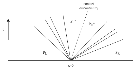
The Riemann Problem of the GPR model takes the form demonstrated in Figure 5 on page 5. Assuming all waves are distinct, there are four waves on either side of the contact discontinuity. On each side, one wave corresponds to the thermal impulse (manifesting as a heat wave) and the other three correspond to the distortion components in the axis in which the Riemann Problem is considered (manifesting as two shear waves and one longitudinal pressure wave). It is important to note that - owing to the source terms - the star states are not constant in the spacetime region in which they reside, so the method presented here produces only an approximation to them.

The method is presented here along the first spatial axis. It can easily be adapted along any axis by taking the components of all relevant vector quantities (velocity, distortion, and thermal impulse) in the direction normal to the interface.
Refer to caption
Figure 5: The Riemann Problem for the GPR model, assuming all waves are distinct

Denote the vector of primitive variables by 𝑷𝑷\boldsymbol{P}. Take the set of left eigenvectors L𝐿L (68) with eigenvalues {λi}subscript𝜆𝑖\left\{\lambda_{i}\right\} . From (54), we have the standard set of relations along characteristics (curves along which dxdt=λi𝑑𝑥𝑑𝑡subscript𝜆𝑖\frac{dx}{dt}=\lambda_{i}):

Ld𝑷=dtL𝑺𝐿𝑑𝑷𝑑𝑡𝐿𝑺L\cdot d\boldsymbol{P}=dt\cdot L\cdot\boldsymbol{S} (94)

In what follows, we enact an operator splitting of the two processes present in the system (94):

Ld𝑷𝐿𝑑𝑷\displaystyle L\cdot d\boldsymbol{P} =𝟎absent0\displaystyle=\boldsymbol{0} (95a)
d𝑷dt𝑑𝑷𝑑𝑡\displaystyle\frac{d\boldsymbol{P}}{dt} =𝑺absent𝑺\displaystyle=\boldsymbol{S} (95b)

𝑷𝑲superscript𝑷absent𝑲\boldsymbol{P^{*K}} is now sought, where K=L𝐾𝐿K=L or K=R𝐾𝑅K=R, denoting the left or right sides of the interface, respectively. Take the following linearization:

d𝑷𝑲𝑷𝑲𝑷𝑲𝑑superscript𝑷𝑲superscript𝑷absent𝑲superscript𝑷𝑲d\boldsymbol{P^{K}}\approx\boldsymbol{P^{*K}}-\boldsymbol{P^{K}} (96)
Refer to caption
Figure 6: Different sets of characteristic curves, traveling from their respective initial points to the star region

13 relations from (95a) are taken: 4 regarding the 4 sets of characteristics traveling into the contact discontinuity from side K𝐾K (with speeds greater or less than v𝑣v for K=L𝐾𝐿K=L or K=R𝐾𝑅K=R, respectively), and 9 relating to the contact discontinuity itself. This is demonstrated in Figure 6 on page 6. 4 more relations must be derived to solve the system for 𝑷𝑲superscript𝑷absent𝑲\boldsymbol{P^{*K}}.

Define the total stress tensor as:

ΣpIσΣ𝑝𝐼𝜎\Sigma\equiv pI-\sigma (97)

The values of Σ,TΣ𝑇\Sigma,T under variables 𝑷𝑲superscript𝑷absent𝑲\boldsymbol{P^{*K}} are obtained by expanding the following Taylor series:

ΣsuperscriptΣ\displaystyle\Sigma^{*} =Σ+(ρρ)Σρ+(pp)Σp+(AmnAmn)ΣAmn+O(d𝑷2)absentΣsuperscript𝜌𝜌Σ𝜌superscript𝑝𝑝Σ𝑝superscriptsubscript𝐴𝑚𝑛subscript𝐴𝑚𝑛Σsubscript𝐴𝑚𝑛𝑂𝑑superscript𝑷2\displaystyle=\Sigma+\left(\rho^{*}-\rho\right)\frac{\partial\Sigma}{\partial\rho}+\left(p^{*}-p\right)\frac{\partial\Sigma}{\partial p}+\left(A_{mn}^{*}-A_{mn}\right)\frac{\partial\Sigma}{\partial A_{mn}}+O\left(d\boldsymbol{P}^{2}\right) (98a)
Tsuperscript𝑇\displaystyle T^{*} =T+(ρρ)Tρ+(pp)Tp+O(d𝑷2)absent𝑇superscript𝜌𝜌𝑇𝜌superscript𝑝𝑝𝑇𝑝𝑂𝑑superscript𝑷2\displaystyle=T+\left(\rho^{*}-\rho\right)\frac{\partial T}{\partial\rho}+\left(p^{*}-p\right)\frac{\partial T}{\partial p}+O\left(d\boldsymbol{P}^{2}\right) (98b)

Thus, we have:

ΣΣsuperscriptΣΣ\displaystyle\Sigma^{*}-\Sigma (pp)I(ρρ)σρ(AmnAmn)σAmnabsentsuperscript𝑝𝑝𝐼superscript𝜌𝜌𝜎𝜌superscriptsubscript𝐴𝑚𝑛subscript𝐴𝑚𝑛𝜎subscript𝐴𝑚𝑛\displaystyle\approx\left(p^{*}-p\right)I-\left(\rho^{*}-\rho\right)\frac{\partial\sigma}{\partial\rho}-\left(A_{mn}^{*}-A_{mn}\right)\frac{\partial\sigma}{\partial A_{mn}} (99a)
TTsuperscript𝑇𝑇\displaystyle T^{*}-T (ρρ)Tρ+(pp)Tpabsentsuperscript𝜌𝜌𝑇𝜌superscript𝑝𝑝𝑇𝑝\displaystyle\approx\left(\rho^{*}-\rho\right)\frac{\partial T}{\partial\rho}+\left(p^{*}-p\right)\frac{\partial T}{\partial p} (99b)

These are the extra required relations. Thus we have:

L^K(𝑷𝑲𝑷𝑲)=𝒄𝑲superscript^𝐿𝐾superscript𝑷absent𝑲superscript𝑷𝑲superscript𝒄𝑲\hat{L}^{K}\cdot\left(\boldsymbol{P^{*K}}-\boldsymbol{P^{K}}\right)=\boldsymbol{c^{K}} (100)

where L^Ksuperscript^𝐿𝐾\hat{L}^{K} takes the form found in (115), with ξ=1𝜉1\xi=-1 for K=R𝐾𝑅K=R and ξ=1𝜉1\xi=1 for K=L𝐾𝐿K=L, and:

𝒄𝑲=(𝚺𝟏𝑲𝚺𝟏𝑲TKTK𝟎)superscript𝒄𝑲superscriptsubscript𝚺1absent𝑲superscriptsubscript𝚺1𝑲superscript𝑇absent𝐾superscript𝑇𝐾0\boldsymbol{c^{K}}=\left(\begin{array}[]{c}\boldsymbol{\Sigma_{1}^{*K}}-\boldsymbol{\Sigma_{1}^{K}}\\ T^{*K}-T^{K}\\ \boldsymbol{0}\end{array}\right) (101)

The inverse of L^Ksuperscript^𝐿𝐾\hat{L}^{K} takes the form found in (116).

L^K,L^K1\hat{L}^{K},\hat{L}^{K}{}^{-1} are evaluated at 𝑷𝑲superscript𝑷𝑲\boldsymbol{P^{K}}. It remains to find expressions for ΣsuperscriptΣ\Sigma^{*} and Tsuperscript𝑇T^{*} in terms of 𝑷𝑳,𝑷𝑹superscript𝑷𝑳superscript𝑷𝑹\boldsymbol{P^{L}},\boldsymbol{P^{R}} to close the system. The obtained values depend on the boundary conditions chosen, as explained below.

2.2.1 Boundary Conditions

Stick Boundary Conditions

The following boundary conditions are used:

𝚺𝟏𝑳superscriptsubscript𝚺1absent𝑳\displaystyle\boldsymbol{\Sigma_{1}^{*L}} =𝚺𝟏𝑹absentsuperscriptsubscript𝚺1absent𝑹\displaystyle=\boldsymbol{\Sigma_{1}^{*R}} (102a)
TLsuperscript𝑇absent𝐿\displaystyle T^{*L} =TRabsentsuperscript𝑇absent𝑅\displaystyle=T^{*R} (102b)
𝒗𝑳superscript𝒗absent𝑳\displaystyle\boldsymbol{v^{*L}} =𝒗𝑹absentsuperscript𝒗absent𝑹\displaystyle=\boldsymbol{v^{*R}} (102c)
q1Lsuperscriptsubscript𝑞1absent𝐿\displaystyle q_{1}^{*L} =q1Rabsentsuperscriptsubscript𝑞1absent𝑅\displaystyle=q_{1}^{*R} (102d)

Taking the relevant rows of 𝑷𝑲=𝑷𝑲+L^K𝒄𝑲1superscript𝑷absent𝑲superscript𝑷𝑲superscript^𝐿𝐾superscriptsuperscript𝒄𝑲1\boldsymbol{P^{*K}}=\boldsymbol{P^{K}}+\hat{L}^{K}{}^{-1}\boldsymbol{c^{K}}:

(𝒗J1)=(𝒗𝑲J1K)+YK((𝚺𝟏T)(𝚺𝟏𝑲TK))superscript𝒗superscriptsubscript𝐽1superscript𝒗𝑲superscriptsubscript𝐽1𝐾superscript𝑌𝐾superscriptsubscript𝚺1superscript𝑇superscriptsubscript𝚺1𝑲superscript𝑇𝐾\left(\begin{array}[]{c}\boldsymbol{v^{*}}\\ J_{1}^{*}\end{array}\right)=\left(\begin{array}[]{c}\boldsymbol{v^{K}}\\ J_{1}^{K}\end{array}\right)+Y^{K}\left(\left(\begin{array}[]{c}\boldsymbol{\Sigma_{1}^{*}}\\ T^{*}\end{array}\right)-\left(\begin{array}[]{c}\boldsymbol{\Sigma_{1}^{K}}\\ T^{K}\end{array}\right)\right) (103)

Thus:

(𝚺𝟏T)=(YLYR)1((𝒗𝑹J1R)(𝒗𝑳J1L)+YL(𝚺𝟏𝑳TL)YR(𝚺𝟏𝑹TR))superscriptsubscript𝚺1superscript𝑇superscriptsuperscript𝑌𝐿superscript𝑌𝑅1superscript𝒗𝑹superscriptsubscript𝐽1𝑅superscript𝒗𝑳superscriptsubscript𝐽1𝐿superscript𝑌𝐿superscriptsubscript𝚺1𝑳superscript𝑇𝐿superscript𝑌𝑅superscriptsubscript𝚺1𝑹superscript𝑇𝑅\left(\begin{array}[]{c}\boldsymbol{\Sigma_{1}^{*}}\\ T^{*}\end{array}\right)=\left(Y^{L}-Y^{R}\right)^{-1}\left(\begin{array}[]{c}\left(\begin{array}[]{c}\boldsymbol{v^{R}}\\ J_{1}^{R}\end{array}\right)-\left(\begin{array}[]{c}\boldsymbol{v^{L}}\\ J_{1}^{L}\end{array}\right)+Y^{L}\left(\begin{array}[]{c}\boldsymbol{\Sigma_{1}^{L}}\\ T^{L}\end{array}\right)-Y^{R}\left(\begin{array}[]{c}\boldsymbol{\Sigma_{1}^{R}}\\ T^{R}\end{array}\right)\end{array}\right) (104)
Slip Boundary Conditions

The following boundary conditions are used:

Σ11LsuperscriptsubscriptΣ11absent𝐿\displaystyle\Sigma_{11}^{*L} =Σ11RabsentsuperscriptsubscriptΣ11absent𝑅\displaystyle=\Sigma_{11}^{*R} (105a)
Σ12L,Σ12RsuperscriptsubscriptΣ12absent𝐿superscriptsubscriptΣ12absent𝑅\displaystyle\Sigma_{12}^{*L},\Sigma_{12}^{*R} =0absent0\displaystyle=0 (105b)
Σ13L,Σ13RsuperscriptsubscriptΣ13absent𝐿superscriptsubscriptΣ13absent𝑅\displaystyle\Sigma_{13}^{*L},\Sigma_{13}^{*R} =0absent0\displaystyle=0 (105c)
TLsuperscript𝑇absent𝐿\displaystyle T^{*L} =TRabsentsuperscript𝑇absent𝑅\displaystyle=T^{*R} (105d)
v1Lsuperscriptsubscript𝑣1absent𝐿\displaystyle v_{1}^{*L} =v1Rabsentsuperscriptsubscript𝑣1absent𝑅\displaystyle=v_{1}^{*R} (105e)
q1Lsuperscriptsubscript𝑞1absent𝐿\displaystyle q_{1}^{*L} =q1Rabsentsuperscriptsubscript𝑞1absent𝑅\displaystyle=q_{1}^{*R} (105f)

Taking the relevant rows of 𝑷𝑲=𝑷𝑲+L^K𝒄𝑲1superscript𝑷absent𝑲superscript𝑷𝑲superscript^𝐿𝐾superscriptsuperscript𝒄𝑲1\boldsymbol{P^{*K}}=\boldsymbol{P^{K}}+\hat{L}^{K}{}^{-1}\boldsymbol{c^{K}}:

(v1J1)=(v1KJ1K)+Y~K((Σ1100T)(Σ11KΣ12KΣ13KTK))superscriptsubscript𝑣1superscriptsubscript𝐽1superscriptsubscript𝑣1𝐾superscriptsubscript𝐽1𝐾superscript~𝑌𝐾superscriptsubscriptΣ1100superscript𝑇superscriptsubscriptΣ11𝐾superscriptsubscriptΣ12𝐾superscriptsubscriptΣ13𝐾superscript𝑇𝐾\left(\begin{array}[]{c}v_{1}^{*}\\ J_{1}^{*}\end{array}\right)=\left(\begin{array}[]{c}v_{1}^{K}\\ J_{1}^{K}\end{array}\right)+\tilde{Y}^{K}\left(\left(\begin{array}[]{c}\Sigma_{11}^{*}\\ 0\\ 0\\ T^{*}\end{array}\right)-\left(\begin{array}[]{c}\Sigma_{11}^{K}\\ \Sigma_{12}^{K}\\ \Sigma_{13}^{K}\\ T^{K}\end{array}\right)\right) (106)

where

Y~K=(𝒀𝟏𝑲𝒀𝟒𝑲)superscript~𝑌𝐾superscriptsubscript𝒀1𝑲superscriptsubscript𝒀4𝑲\tilde{Y}^{K}=\left(\begin{array}[]{c}\boldsymbol{Y_{1}^{K}}\\ \boldsymbol{Y_{4}^{K}}\end{array}\right) (107)

Thus:

(Σ11T)=(Y^LY^R)1((v1RJ1R)(v1KJ1L)+YL(𝚺𝟏𝑳TL)YR(𝚺𝟏𝑹TR))superscriptsubscriptΣ11superscript𝑇superscriptsuperscript^𝑌𝐿superscript^𝑌𝑅1superscriptsubscript𝑣1𝑅superscriptsubscript𝐽1𝑅superscriptsubscript𝑣1𝐾superscriptsubscript𝐽1𝐿superscript𝑌𝐿superscriptsubscript𝚺1𝑳superscript𝑇𝐿superscript𝑌𝑅superscriptsubscript𝚺1𝑹superscript𝑇𝑅\left(\begin{array}[]{c}\Sigma_{11}^{*}\\ T^{*}\end{array}\right)=\left(\hat{Y}^{L}-\hat{Y}^{R}\right)^{-1}\left(\begin{array}[]{c}\left(\begin{array}[]{c}v_{1}^{R}\\ J_{1}^{R}\end{array}\right)-\left(\begin{array}[]{c}v_{1}^{K}\\ J_{1}^{L}\end{array}\right)+Y^{L}\left(\begin{array}[]{c}\boldsymbol{\Sigma_{1}^{L}}\\ T^{L}\end{array}\right)-Y^{R}\left(\begin{array}[]{c}\boldsymbol{\Sigma_{1}^{R}}\\ T^{R}\end{array}\right)\end{array}\right) (108)

where

Y^K=(Y11KY14KY41KY44K)superscript^𝑌𝐾superscriptsubscript𝑌11𝐾superscriptsubscript𝑌14𝐾superscriptsubscript𝑌41𝐾superscriptsubscript𝑌44𝐾\hat{Y}^{K}=\left(\begin{array}[]{cc}Y_{11}^{K}&Y_{14}^{K}\\ Y_{41}^{K}&Y_{44}^{K}\end{array}\right) (109)
Vacuum Boundary Conditions

The following boundary conditions are used:

𝚺𝟏superscriptsubscript𝚺1\displaystyle\boldsymbol{\Sigma_{1}^{*}} =𝟎absent0\displaystyle=\boldsymbol{0} (110a)
q1superscriptsubscript𝑞1\displaystyle q_{1}^{*} =0absent0\displaystyle=0 (110b)

Taking the relevant row of 𝑷𝑲=𝑷𝑲+L^K𝒄𝑲1superscript𝑷absent𝑲superscript𝑷𝑲superscript^𝐿𝐾superscriptsuperscript𝒄𝑲1\boldsymbol{P^{*K}}=\boldsymbol{P^{K}}+\hat{L}^{K}{}^{-1}\boldsymbol{c^{K}}:

J1=J1K+𝒀𝟒𝑲((𝟎T)(𝚺𝟏𝑲TK))superscriptsubscript𝐽1superscriptsubscript𝐽1𝐾superscriptsubscript𝒀4𝑲0superscript𝑇superscriptsubscript𝚺1𝑲superscript𝑇𝐾J_{1}^{*}=J_{1}^{K}+\boldsymbol{Y_{4}^{K}}\cdot\left(\left(\begin{array}[]{c}\boldsymbol{0}\\ T^{*}\end{array}\right)-\left(\begin{array}[]{c}\boldsymbol{\Sigma_{1}^{K}}\\ T^{K}\end{array}\right)\right) (111)

As q1=0superscriptsubscript𝑞10q_{1}^{*}=0 implies that J1=0superscriptsubscript𝐽10J_{1}^{*}=0, we have:

T=1Y44K(𝒀𝟒𝑲(𝚺𝟏𝑲TK)J1K)=TK+𝒀𝟒,:𝟑𝑲𝚺𝟏𝑲J1KY44Ksuperscript𝑇1superscriptsubscript𝑌44𝐾superscriptsubscript𝒀4𝑲superscriptsubscript𝚺1𝑲superscript𝑇𝐾superscriptsubscript𝐽1𝐾superscript𝑇𝐾superscriptsubscript𝒀4bold-:absent3𝑲superscriptsubscript𝚺1𝑲superscriptsubscript𝐽1𝐾superscriptsubscript𝑌44𝐾T^{*}=\frac{1}{Y_{44}^{K}}\left(\boldsymbol{Y_{4}^{K}}\cdot\left(\begin{array}[]{c}\boldsymbol{\Sigma_{1}^{K}}\\ T^{K}\end{array}\right)-J_{1}^{K}\right)=T^{K}+\frac{\boldsymbol{Y_{4,:3}^{K}}\cdot\boldsymbol{\Sigma_{1}^{K}}-J_{1}^{K}}{Y_{44}^{K}} (112)
Iteration

(100) is solved for 𝑷𝑲superscript𝑷absent𝑲\boldsymbol{P^{*K}}, which is taken to be the star state if the following conditions are satisfied:

|𝚺𝟏𝑳𝚺𝟏𝑹|min(ρ0L,ρ0R)×min(csL,csR)2\displaystyle\frac{\left|\boldsymbol{\Sigma_{1}^{*L}}-\boldsymbol{\Sigma_{1}^{*R}}\right|}{\min\left(\rho_{0}^{L},\rho_{0}^{R}\right)\times\min\left(c_{s}^{L},c_{s}^{R}\right)^{2}} <TOLabsent𝑇𝑂𝐿\displaystyle<TOL (113a)
|v1Lv1R|min(csL,csR)superscriptsubscript𝑣1𝐿superscriptsubscript𝑣1𝑅superscriptsubscript𝑐𝑠𝐿superscriptsubscript𝑐𝑠𝑅\displaystyle\frac{\left|v_{1}^{L}-v_{1}^{R}\right|}{\min\left(c_{s}^{L},c_{s}^{R}\right)} <TOLabsent𝑇𝑂𝐿\displaystyle<TOL (113b)
|q1Lq1R|min(q~L,q~R)superscriptsubscript𝑞1𝐿superscriptsubscript𝑞1𝑅superscript~𝑞𝐿superscript~𝑞𝑅\displaystyle\frac{\left|q_{1}^{L}-q_{1}^{R}\right|}{\min\left(\tilde{q}^{L},\tilde{q}^{R}\right)} <TOLabsent𝑇𝑂𝐿\displaystyle<TOL (113c)
|TLTR|min(T0L,T0R)superscript𝑇𝐿superscript𝑇𝑅superscriptsubscript𝑇0𝐿superscriptsubscript𝑇0𝑅\displaystyle\frac{\left|T^{L}-T^{R}\right|}{\min\left(T_{0}^{L},T_{0}^{R}\right)} <TOLabsent𝑇𝑂𝐿\displaystyle<TOL (113d)

where

q~=ct2ρ0T03cV~𝑞superscriptsubscript𝑐𝑡2subscript𝜌0superscriptsubscript𝑇03subscript𝑐𝑉\tilde{q}=\frac{c_{t}^{2}}{\rho_{0}}\sqrt{\frac{T_{0}^{3}}{c_{V}}} (114)

These convergence criteria are chosen so that the variables required to be less than TOL𝑇𝑂𝐿TOL are dimensionless. At every iteration, (95b) is solved using the ODE solvers presented in [32, 33].

2.2.2 Linear Conditions with Heat Conduction

We now obtain L^Ksuperscript^𝐿𝐾\hat{L}^{K} and its inverse in order to solve (100). Replacing the first four lines of (68) with the conditions (99a), (99b), we have:

L^K={(𝝈𝒅ρ𝒆𝒅Π1Π2Π303,6TρTp01,301,301,301,6)(QΞ11ρQ:,1:3Π21ρQ:,1:3Π3ξDQ04,2)(1ρ0𝒆𝒅𝑻A1𝒆𝒅𝑻A1Π11Π2𝒆𝒅𝑻A1Π11Π301,6)(03,5I303,303,603,503,3I303,6)(02,15I2)}superscript^𝐿𝐾subscript𝝈𝒅𝜌subscript𝒆𝒅subscriptΠ1subscriptΠ2subscriptΠ3subscript036𝑇𝜌𝑇𝑝subscript013subscript013subscript013subscript016𝑄subscriptΞ11𝜌subscript𝑄::13subscriptΠ21𝜌subscript𝑄::13subscriptΠ3𝜉𝐷𝑄subscript0421𝜌0superscriptsubscript𝒆𝒅𝑻superscript𝐴1superscriptsubscript𝒆𝒅𝑻superscript𝐴1superscriptsubscriptΠ11subscriptΠ2superscriptsubscript𝒆𝒅𝑻superscript𝐴1superscriptsubscriptΠ11subscriptΠ3subscript016subscript035subscript𝐼3subscript033subscript036subscript035subscript033subscript𝐼3subscript036subscript0215subscript𝐼2\hat{L}^{K}=\left\{\begin{array}[]{c}\left(\begin{array}[]{cccccc}-\frac{\partial\boldsymbol{\sigma_{d}}}{\partial\rho}&\boldsymbol{e_{d}}&-\Pi_{1}&-\Pi_{2}&-\Pi_{3}&0_{3,6}\\ \frac{\partial T}{\partial\rho}&\frac{\partial T}{\partial p}&0_{1,3}&0_{1,3}&0_{1,3}&0_{1,6}\end{array}\right)\\ \left(\begin{array}[]{ccccc}Q\Xi_{1}&-\frac{1}{\rho}Q_{:,1:3}\Pi_{2}&-\frac{1}{\rho}Q_{:,1:3}\Pi_{3}&\xi DQ&0_{4,2}\end{array}\right)\\ \left(\begin{array}[]{cccccc}-\frac{1}{\rho}&0&\boldsymbol{e_{d}^{T}}A^{-1}&\boldsymbol{e_{d}^{T}}A^{-1}\Pi_{1}^{-1}\Pi_{2}&\boldsymbol{e_{d}^{T}}A^{-1}\Pi_{1}^{-1}\Pi_{3}&0_{1,6}\end{array}\right)\\ \left(\begin{array}[]{cccc}0_{3,5}&I_{3}&0_{3,3}&0_{3,6}\\ 0_{3,5}&0_{3,3}&I_{3}&0_{3,6}\end{array}\right)\\ \left(\begin{array}[]{cc}0_{2,15}&I_{2}\end{array}\right)\end{array}\right\} (115)

Thus, the inverse of the left-eigenvector matrix becomes:

L^K=1{(X1I5,406,4Y02,4),(011,4ξ(DQ)102,4),(cTpcTρcΠd1𝒘012,1),(02,302,3Π11Π2Π11Π3I303,303,3I306,306,3),(015,2I2)}\hat{L}^{K}{}^{-1}=\left\{\left(\begin{array}[]{c}X^{-1}I_{5,4}\\ 0_{6,4}\\ Y\\ 0_{2,4}\end{array}\right),\left(\begin{array}[]{c}0_{11,4}\\ \xi\left(DQ\right)^{-1}\\ 0_{2,4}\end{array}\right),\left(\begin{array}[]{c}-cT_{p}\\ cT_{\rho}\\ c\Pi_{d}^{-1}\boldsymbol{w}\\ 0_{12,1}\end{array}\right),\left(\begin{array}[]{cc}0_{2,3}&0_{2,3}\\ -\Pi_{1}^{-1}\Pi_{2}&-\Pi_{1}^{-1}\Pi_{3}\\ I_{3}&0_{3,3}\\ 0_{3,3}&I_{3}\\ 0_{6,3}&0_{6,3}\end{array}\right),\left(\begin{array}[]{c}0_{15,2}\\ I_{2}\end{array}\right)\right\} (116)

where:

X=(B~11B~12(Π1)11(Π1)12(Π1)13B~21B~22(Π1)21(Π1)22(Π1)23B~31B~32(Π1)31(Π1)32(Π1)33D~11D~12C~11C~12C~13D~21D~22C~21C~22C~23)𝑋subscript~𝐵11subscript~𝐵12subscriptsubscriptΠ111subscriptsubscriptΠ112subscriptsubscriptΠ113subscript~𝐵21subscript~𝐵22subscriptsubscriptΠ121subscriptsubscriptΠ122subscriptsubscriptΠ123subscript~𝐵31subscript~𝐵32subscriptsubscriptΠ131subscriptsubscriptΠ132subscriptsubscriptΠ133subscript~𝐷11subscript~𝐷12subscript~𝐶11subscript~𝐶12subscript~𝐶13subscript~𝐷21subscript~𝐷22subscript~𝐶21subscript~𝐶22subscript~𝐶23X=\left(\begin{array}[]{ccccc}\tilde{B}_{11}&\tilde{B}_{12}&\left(-\Pi_{1}\right)_{11}&\left(-\Pi_{1}\right)_{12}&\left(-\Pi_{1}\right)_{13}\\ \tilde{B}_{21}&\tilde{B}_{22}&\left(-\Pi_{1}\right)_{21}&\left(-\Pi_{1}\right)_{22}&\left(-\Pi_{1}\right)_{23}\\ \tilde{B}_{31}&\tilde{B}_{32}&\left(-\Pi_{1}\right)_{31}&\left(-\Pi_{1}\right)_{32}&\left(-\Pi_{1}\right)_{33}\\ \tilde{D}_{11}&\tilde{D}_{12}&\tilde{C}_{11}&\tilde{C}_{12}&\tilde{C}_{13}\\ \tilde{D}_{21}&\tilde{D}_{22}&\tilde{C}_{21}&\tilde{C}_{22}&\tilde{C}_{23}\end{array}\right) (117a)
Y=ξQ1D1QΞ1X1I5,4𝑌𝜉superscript𝑄1superscript𝐷1𝑄subscriptΞ1superscript𝑋1subscript𝐼54Y=-\xi Q^{-1}D^{-1}Q\Xi_{1}X^{-1}I_{5,4} (117b)

and also:

B~=(𝝈𝒅ρ𝒆𝒅)~𝐵subscript𝝈𝒅𝜌subscript𝒆𝒅\tilde{B}=\left(\begin{array}[]{cc}-\frac{\partial\boldsymbol{\sigma_{d}}}{\partial\rho}&\boldsymbol{e_{d}}\end{array}\right) (118a)
C~=(000Ad11Ad21Ad31)~𝐶000superscriptsubscript𝐴𝑑11superscriptsubscript𝐴𝑑21superscriptsubscript𝐴𝑑31\tilde{C}=\left(\begin{array}[]{ccc}0&0&0\\ A_{d1}^{-1}&A_{d2}^{-1}&A_{d3}^{-1}\end{array}\right) (118b)
D~=(TρTp1ρ0)~𝐷𝑇𝜌𝑇𝑝1𝜌0\tilde{D}=\left(\begin{array}[]{cc}\frac{\partial T}{\partial\rho}&\frac{\partial T}{\partial p}\\ -\frac{1}{\rho}&0\end{array}\right) (118c)

By inversion of block matrices555(ABCD)1=((ABD1C)1(ABD1C)1BD1D1C(ABD1C)1D1(I+C(ABD1C)1BD1))superscript𝐴𝐵𝐶𝐷1superscript𝐴𝐵superscript𝐷1𝐶1superscript𝐴𝐵superscript𝐷1𝐶1𝐵superscript𝐷1superscript𝐷1𝐶superscript𝐴𝐵superscript𝐷1𝐶1superscript𝐷1𝐼𝐶superscript𝐴𝐵superscript𝐷1𝐶1𝐵superscript𝐷1\left(\begin{array}[]{cc}A&B\\ C&D\end{array}\right)^{-1}=\left(\begin{array}[]{cc}\left(A-BD^{-1}C\right)^{-1}&-\left(A-BD^{-1}C\right)^{-1}BD^{-1}\\ -D^{-1}C\left(A-BD^{-1}C\right)^{-1}&D^{-1}\left(I+C\left(A-BD^{-1}C\right)^{-1}BD^{-1}\right)\end{array}\right):

X1=(D~1C~Z1D~1(IC~Z1B~D~1)Z1Z1B~D~1)superscript𝑋1superscript~𝐷1~𝐶superscript𝑍1superscript~𝐷1𝐼~𝐶superscript𝑍1~𝐵superscript~𝐷1superscript𝑍1superscript𝑍1~𝐵superscript~𝐷1X^{-1}=\left(\begin{array}[]{cc}\tilde{D}^{-1}\tilde{C}Z^{-1}&\tilde{D}^{-1}\left(I-\tilde{C}Z^{-1}\tilde{B}\tilde{D}^{-1}\right)\\ -Z^{-1}&Z^{-1}\tilde{B}\tilde{D}^{-1}\end{array}\right) (119)

where

Z=Π1+ρTp(Tp𝝈𝒅ρ+Tρ𝒆𝒅)𝒆𝒅𝑻A1𝑍subscriptΠ1𝜌subscript𝑇𝑝subscript𝑇𝑝subscript𝝈𝒅𝜌subscript𝑇𝜌subscript𝒆𝒅superscriptsubscript𝒆𝒅𝑻superscript𝐴1Z=\Pi_{1}+\frac{\rho}{T_{p}}\left(T_{p}\frac{\partial\boldsymbol{\sigma_{d}}}{\partial\rho}+T_{\rho}\boldsymbol{e_{d}}\right)\boldsymbol{e_{d}^{T}}A^{-1} (120)

2.2.3 Linear Conditions without Heat Conduction

If the heat conduction terms are dropped from the GPR model, the eigenstructure of the system changes, along with the solution of the linear conditions. ΞΞ\Xi retains the same definition, but is now a 3×3333\times 3 matrix (comprising the top-left corner of ΞΞ\Xi under heat conduction). Thus, Q,D𝑄𝐷Q,D are also 3×3333\times 3 matrices. Taking the eigenvectors (93), the linear conditions become:

L^K={(𝝈𝒅ρ𝒆𝒅Π1Π2Π3)(QΞ11ρQΠ21ρQΠ3ξDQ)(IBA1C)1(I2BA1BA1Π11Π2BA1Π11Π302,3)(03,5I303,303,303,503,3I303,3)}superscript^𝐿𝐾subscript𝝈𝒅𝜌subscript𝒆𝒅subscriptΠ1subscriptΠ2subscriptΠ3𝑄subscriptΞ11𝜌𝑄subscriptΠ21𝜌𝑄subscriptΠ3𝜉𝐷𝑄superscript𝐼𝐵superscript𝐴1𝐶1subscript𝐼2𝐵superscript𝐴1𝐵superscript𝐴1superscriptsubscriptΠ11subscriptΠ2𝐵superscript𝐴1superscriptsubscriptΠ11subscriptΠ3subscript023subscript035subscript𝐼3subscript033subscript033subscript035subscript033subscript𝐼3subscript033\hat{L}^{K}=\left\{\begin{array}[]{c}\left(\begin{array}[]{ccccc}-\frac{\partial\boldsymbol{\sigma_{d}}}{\partial\rho}&\boldsymbol{e_{d}}&-\Pi_{1}&-\Pi_{2}&-\Pi_{3}\end{array}\right)\\ \left(\begin{array}[]{cccc}Q\Xi_{1}&-\frac{1}{\rho}Q\Pi_{2}&-\frac{1}{\rho}Q\Pi_{3}&\xi DQ\end{array}\right)\\ \left(I-BA^{-1}C\right)^{-1}\left(\begin{array}[]{ccccc}I_{2}&-BA^{-1}&-BA^{-1}\Pi_{1}^{-1}\Pi_{2}&-BA^{-1}\Pi_{1}^{-1}\Pi_{3}&0_{2,3}\end{array}\right)\\ \left(\begin{array}[]{cccc}0_{3,5}&I_{3}&0_{3,3}&0_{3,3}\\ 0_{3,5}&0_{3,3}&I_{3}&0_{3,3}\end{array}\right)\end{array}\right\} (121)
L^K=1{(X1I5,406,3Y),(011,3ξ(DQ)1),(1001Π11𝝈𝟏ρΠ11𝒆𝟏𝟎𝟗𝟎𝟗),(02,302,3Π11Π2Π11Π3I303,303,3I303,303,3)}\hat{L}^{K}{}^{-1}=\left\{\left(\begin{array}[]{c}X^{-1}I_{5,4}\\ 0_{6,3}\\ Y\end{array}\right),\left(\begin{array}[]{c}0_{11,3}\\ \xi\left(DQ\right)^{-1}\end{array}\right),\left(\begin{array}[]{cc}1&0\\ 0&1\\ -\Pi_{1}^{-1}\frac{\partial\boldsymbol{\sigma_{1}}}{\partial\rho}&\Pi_{1}^{-1}\boldsymbol{e_{1}}\\ \boldsymbol{0_{9}}&\boldsymbol{0_{9}}\end{array}\right),\left(\begin{array}[]{cc}0_{2,3}&0_{2,3}\\ -\Pi_{1}^{-1}\Pi_{2}&-\Pi_{1}^{-1}\Pi_{3}\\ I_{3}&0_{3,3}\\ 0_{3,3}&I_{3}\\ 0_{3,3}&0_{3,3}\end{array}\right)\right\} (122)

where:

X=(B~11B~12(Π1)11(Π1)12(Π1)13B~21B~22(Π1)21(Π1)22(Π1)23B~31B~32(Π1)31(Π1)32(Π1)33Δ111Δ121(Δ1BA1)11(Δ1BA1)12(Δ1BA1)13Δ211Δ221(Δ1BA1)21(Δ1BA1)22(Δ1BA1)23)𝑋subscript~𝐵11subscript~𝐵12subscriptsubscriptΠ111subscriptsubscriptΠ112subscriptsubscriptΠ113subscript~𝐵21subscript~𝐵22subscriptsubscriptΠ121subscriptsubscriptΠ122subscriptsubscriptΠ123subscript~𝐵31subscript~𝐵32subscriptsubscriptΠ131subscriptsubscriptΠ132subscriptsubscriptΠ133superscriptsubscriptΔ111superscriptsubscriptΔ121subscriptsuperscriptΔ1𝐵superscript𝐴111subscriptsuperscriptΔ1𝐵superscript𝐴112subscriptsuperscriptΔ1𝐵superscript𝐴113superscriptsubscriptΔ211superscriptsubscriptΔ221subscriptsuperscriptΔ1𝐵superscript𝐴121subscriptsuperscriptΔ1𝐵superscript𝐴122subscriptsuperscriptΔ1𝐵superscript𝐴123X=\left(\begin{array}[]{ccccc}\tilde{B}_{11}&\tilde{B}_{12}&\left(-\Pi_{1}\right)_{11}&\left(-\Pi_{1}\right)_{12}&\left(-\Pi_{1}\right)_{13}\\ \tilde{B}_{21}&\tilde{B}_{22}&\left(-\Pi_{1}\right)_{21}&\left(-\Pi_{1}\right)_{22}&\left(-\Pi_{1}\right)_{23}\\ \tilde{B}_{31}&\tilde{B}_{32}&\left(-\Pi_{1}\right)_{31}&\left(-\Pi_{1}\right)_{32}&\left(-\Pi_{1}\right)_{33}\\ \Delta_{11}^{-1}&\Delta_{12}^{-1}&\left(-\Delta^{-1}BA^{-1}\right)_{11}&\left(-\Delta^{-1}BA^{-1}\right)_{12}&\left(-\Delta^{-1}BA^{-1}\right)_{13}\\ \Delta_{21}^{-1}&\Delta_{22}^{-1}&\left(-\Delta^{-1}BA^{-1}\right)_{21}&\left(-\Delta^{-1}BA^{-1}\right)_{22}&\left(-\Delta^{-1}BA^{-1}\right)_{23}\end{array}\right) (123a)
Y=ξQ1D1QΞ1X1I5,4𝑌𝜉superscript𝑄1superscript𝐷1𝑄subscriptΞ1superscript𝑋1subscript𝐼54Y=-\xi Q^{-1}D^{-1}Q\Xi_{1}X^{-1}I_{5,4} (123b)

where

ΔΔ\displaystyle\Delta =IBA1Cabsent𝐼𝐵superscript𝐴1𝐶\displaystyle=I-BA^{-1}C (124a)
B~~𝐵\displaystyle\tilde{B} =(𝝈𝟏ρ𝒆𝟏)absentsubscript𝝈1𝜌subscript𝒆1\displaystyle=\left(\begin{array}[]{cc}-\frac{\partial\boldsymbol{\sigma_{1}}}{\partial\rho}&\boldsymbol{e_{1}}\end{array}\right) (124c)
B𝐵\displaystyle B =(ρ00(ρc02+σ11ρσ11ρ)(σ21ρσ21ρ)(σ31ρσ31ρ))absent𝜌00𝜌superscriptsubscript𝑐02subscript𝜎11𝜌subscript𝜎11𝜌subscript𝜎21𝜌subscript𝜎21𝜌subscript𝜎31𝜌subscript𝜎31𝜌\displaystyle=\left(\begin{array}[]{ccc}\rho&0&0\\ \left(\rho c_{0}^{2}+\sigma_{11}-\rho\frac{\partial\sigma_{11}}{\partial\rho}\right)&\left(\sigma_{21}-\rho\frac{\partial\sigma_{21}}{\partial\rho}\right)&\left(\sigma_{31}-\rho\frac{\partial\sigma_{31}}{\partial\rho}\right)\end{array}\right) (124f)

By inversion of block matrices:

X1=(BA1Z~(I+BA1Z~B~)(IBA1Π11B~)Z~Z~B~(IBA1Π11B~))superscript𝑋1𝐵superscript𝐴1~𝑍𝐼𝐵superscript𝐴1~𝑍~𝐵𝐼𝐵superscript𝐴1superscriptsubscriptΠ11~𝐵~𝑍~𝑍~𝐵𝐼𝐵superscript𝐴1superscriptsubscriptΠ11~𝐵X^{-1}=\left(\begin{array}[]{cc}-BA^{-1}\tilde{Z}&\left(I+BA^{-1}\tilde{Z}\tilde{B}\right)\left(I-BA^{-1}\Pi_{1}^{-1}\tilde{B}\right)\\ -\tilde{Z}&\tilde{Z}\tilde{B}\left(I-BA^{-1}\Pi_{1}^{-1}\tilde{B}\right)\end{array}\right) (125)

where

Z~=(Π1B~BA1)1~𝑍superscriptsubscriptΠ1~𝐵𝐵superscript𝐴11\tilde{Z}=\left(\Pi_{1}-\tilde{B}BA^{-1}\right)^{-1} (126)

3 Results

The GPR-RGFM is now assessed. The first fives tests in this chapter are Riemann problems that have appeared elsewhere in the literature. Reference solutions to these problems have been calculated by various methods, as described for each test individually. The sixth test is new; it assess the ability of the GPR-RGFM to correctly model heat conduction across interfaces. The last two tests are well-known two-dimensional problems, to demonstrate the applicability of the method to multiple dimensions. The stiffened gas EOS parameters for three commonly-used fluids are given in Table 1 on page 1.


ρ0subscript𝜌0\rho_{0} cvsubscript𝑐𝑣c_{v} γ𝛾\gamma psubscript𝑝p_{\infty} cssubscript𝑐𝑠c_{s} ctsubscript𝑐𝑡c_{t} μ𝜇\mu Prsubscript𝑃𝑟P_{r}
Air 1.18 718 1.4 - 55 50 1.85×1051.85superscript1051.85\times 10^{-5} 0.714
Helium 0.163 3127 5/3 - 55 50 1.99×1051.99superscript1051.99\times 10^{-5} 0.688
Water 997 950 4.4 6×1086superscript1086\times 10^{8} 1 1 103superscript10310^{-3} 7
Table 1: EOS parameters for different fluids (using SI units)

3.1 Helium Bubble

The interface between two different gases is now modeled. As in Test B of Wang et al. [66], a bubble of helium - surrounded by air - initially occupies the region x[0.4,0.6]𝑥0.40.6x\in\left[0.4,0.6\right]. A shock front in the air, initially at x=0.05𝑥0.05x=0.05, travels towards the helium bubble. The initial conditions are given in Table 2 on page 2 and the EOS parameters for each material are given in Table 1 on page 1.

200 cells are used. Reference solutions are computed using the exact solver for mixed ideal gas Riemann problems under the Euler equations (presented in [64]). The results for times t=7×10⁴𝑡7superscript104t=7\times 10^{-4} and t=14×104𝑡14superscript104t=14\times 10^{-4} are displayed in Figure 7 on page 7. In the former, the shock is about to hit the helium bubble (corresponding to the region of low density). In the latter, the shock has traveled through the helium bubble, compressing it slightly, and the bubble itself has moved almost 0.1 spatial units to the right. There is good correspondence with the results in [66] and the sharp discontinuity in density is maintained.
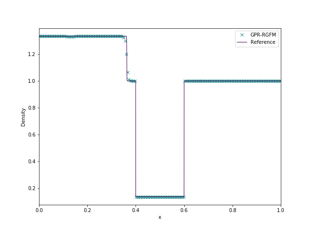
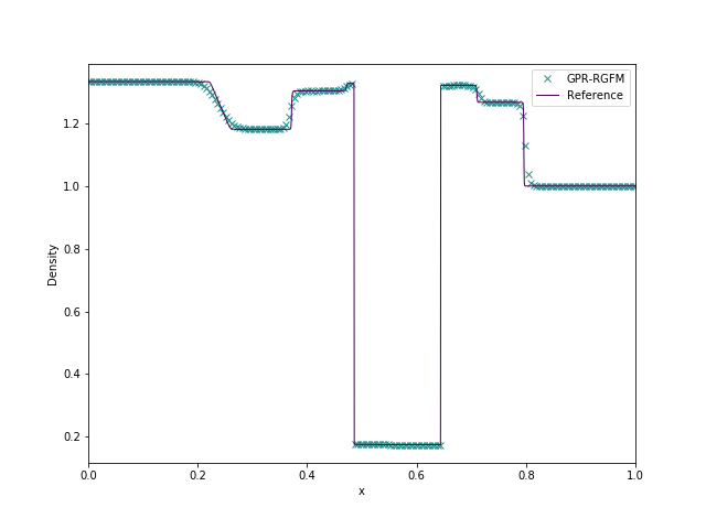
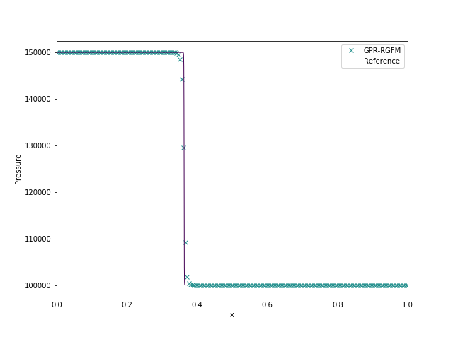
ρ𝜌\rho p𝑝p 𝒗𝒗\boldsymbol{v} A𝐴A 𝑱𝑱\boldsymbol{J}
x<0.05𝑥0.05x<0.05 1.33331.33331.3333 1.5×1051.5superscript1051.5\times 10^{5} (35.351000)35.351000\left(\begin{array}[]{ccc}35.35\sqrt{10}&0&0\end{array}\right) (1.33331.18)13I3superscript1.33331.1813subscript𝐼3\left(\frac{1.3333}{1.18}\right)^{\frac{1}{3}}I_{3} 𝟎0\boldsymbol{0}
0.05x<0.40.05𝑥0.40.05\leq x<0.4 111 105superscript10510^{5} 𝟎0\boldsymbol{0} (11.18)13I3superscript11.1813subscript𝐼3\left(\frac{1}{1.18}\right)^{\frac{1}{3}}I_{3} 𝟎0\boldsymbol{0}
0.4x<0.60.4𝑥0.60.4\leq x<0.6 0.13790.13790.1379 105superscript10510^{5} 𝟎0\boldsymbol{0} (0.13790.163)13I3superscript0.13790.16313subscript𝐼3\left(\frac{0.1379}{0.163}\right)^{\frac{1}{3}}I_{3} 𝟎0\boldsymbol{0}
0.6x10.6𝑥10.6\leq x\leq 1 111 105superscript10510^{5} 𝟎0\boldsymbol{0} (11.18)13I3superscript11.1813subscript𝐼3\left(\frac{1}{1.18}\right)^{\frac{1}{3}}I_{3} 𝟎0\boldsymbol{0}
Table 2: Initial conditions for the helium bubble test
Refer to caption
Refer to caption
Refer to caption
Refer to caption
Refer to caption
Refer to caption
Figure 7: Density, pressure, and velocity for the helium bubble test with GPR-RGFM at times t=7×10⁴𝑡7superscript104t=7\times 10^{-4} (left) and t=14×104𝑡14superscript104t=14\times 10^{-4} (right)

3.2 Water-Air Shock Tube

This test comprises an interface between water and air, with initial data taken from Chinnayya et al. [12] (see Table 3 on page 3). The aim of this test is to evaluate the ability of the GPR-RGFM at capturing interfaces between qualitatively different fluids. The water is initially at high pressure, and the air at atmospheric pressure. Due to the large difference in state variables and qualitative characteristics of the two fluids, this is an example of a test with which the original GFM for the Euler equations does not perform well.

The results using the GPR-RGFM with 200 cells are shown in Figure 8 on page 8, along with the exact solution to the Euler equations (computed using the extension to the stiffened gas equations of the exact Riemann solver presented in [64]). As can be seen, the material interface is captured well, with the correct intermediate density found by the numerical method.
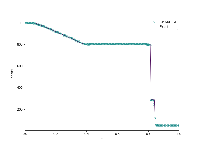
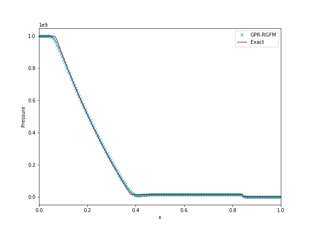
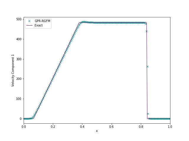
ρ𝜌\rho p𝑝p 𝒗𝒗\boldsymbol{v} A𝐴A 𝑱𝑱\boldsymbol{J}
0x<0.70𝑥0.70\leq x<0.7 100010001000 109superscript10910^{9} 𝟎0\boldsymbol{0} I3subscript𝐼3I_{3} 𝟎0\boldsymbol{0}
0.7x10.7𝑥10.7\leq x\leq 1 505050 105superscript10510^{5} 𝟎0\boldsymbol{0} 503I3350subscript𝐼3\sqrt[3]{50}\cdot I_{3} 𝟎0\boldsymbol{0}
Table 3: Initial conditions for the water-air shock tube test
Refer to caption
Refer to caption
Refer to caption
Refer to caption
Figure 8: Density, pressure, velocity, and internal energy for the water-air shock tube test with GPR-RGFM

3.3 PBX9404-Copper Shock Tube

This test is taken from [7], with the aim of testing the ability of the GPR-RGFM to model interfaces between fluids and solids. High pressure, reacted PBX9404 is in contact with copper at position x=0.5𝑥0.5x=0.5 on domain x[0,1]𝑥01x\in\left[0,1\right], with both materials initially at rest. The pressure of the PBX is initially 18.9GPa18.9𝐺𝑃𝑎18.9GPa, and the entropy of the copper is initially 00. The PBX follows an ideal gas EOS, with parameters ρ0=1840subscript𝜌01840\rho_{0}=1840, γ=2.85𝛾2.85\gamma=2.85, cs=1subscript𝑐𝑠1c_{s}=1, μ=102𝜇superscript102\mu=10^{-2}. The copper follows the Godunov-Romenski EOS, with parameters ρ0=8930subscript𝜌08930\rho_{0}=8930, cv=390subscript𝑐𝑣390c_{v}=390, T0=300subscript𝑇0300T_{0}=300, c0=3939subscript𝑐03939c_{0}=3939, α=1𝛼1\alpha=1, β=3𝛽3\beta=3, γ=2𝛾2\gamma=2, b0=2141subscript𝑏02141b_{0}=2141. The test is run until time t=0.5×10⁶𝑡0.5superscript106t=0.5\times 10^{-6}, using 500 cells.

The exact solution to this test is calculated using the iterative solver described in [4]. The error in the wavespeeds is calculated from the residual error in the traction and velocities across the central contact, as required by the Rankine–Hugoniot conditions and boundary conditions. The wavespeeds are found by iteratively reducing the residual using the Newton–Raphson method.

Plots for density, velocity, and total stress are given in Figure 9 on page 9. As can be seen, the GPR-RGFM is able to reproduce the solution to high fidelity, with a perfectly sharp discontinuity in the density, and a very well resolved discontinuity in the total stress.
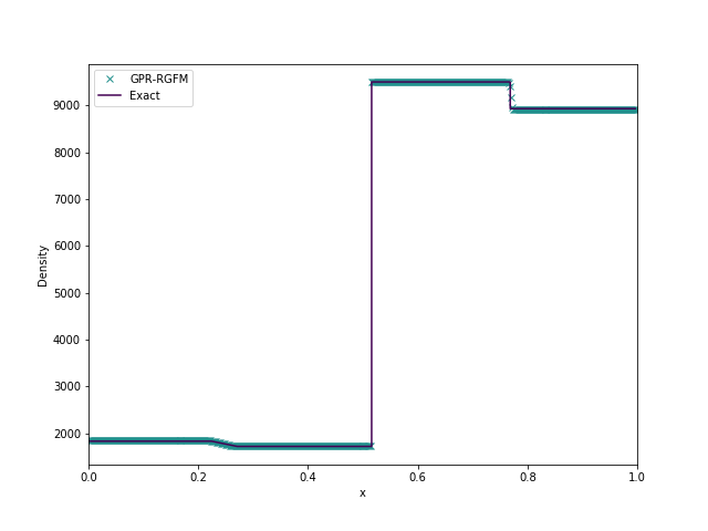
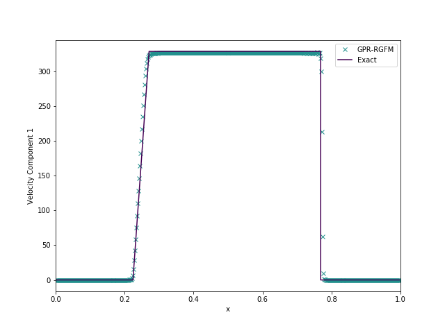
Refer to caption
Refer to caption
Refer to caption
Figure 9: Density, velocity, and total stress for the Copper-PBX test with GPR-RGFM

3.4 Aluminium in Vacuum

This test is taken from [3]. The initial conditions of the test consist of a slab of aluminium, initially with velocity (200.1)200.1\left(\begin{array}[]{ccc}2&0&0.1\end{array}\right), meeting a vacuum at point x=0.5𝑥0.5x=0.5, on the domain x[0,1]𝑥01x\in\left[0,1\right]. The distortion of the aluminium is initially given by:

A=(1000.010.950.020.01500.9)1𝐴superscript1000.010.950.020.01500.91A=\left(\begin{array}[]{ccc}1&0&0\\ -0.01&0.95&0.02\\ -0.015&0&0.9\end{array}\right)^{-1} (127)

The initial density of the aluminium is thus given as ρ=ρ0det(A)𝜌subscript𝜌0𝐴\rho=\rho_{0}\det\left(A\right). The aluminium is modeled using the Godunov-Romenski EOS, with parameters ρ0=2.71subscript𝜌02.71\rho_{0}=2.71, cv=9×10⁴subscript𝑐𝑣9superscript104c_{v}=9\times 10^{-4}, T0=300subscript𝑇0300T_{0}=300, c0=5.037subscript𝑐05.037c_{0}=5.037, α=1𝛼1\alpha=1, β=3.577𝛽3.577\beta=3.577, γ=2.088𝛾2.088\gamma=2.088, b0=3.16subscript𝑏03.16b_{0}=3.16, ct=2subscript𝑐𝑡2c_{t}=2, κ=204𝜅204\kappa=204.

The test was run until time t=0.06𝑡0.06t=0.06, using 500 cells. The results of solving this problem with the GPR-RGFM, not including thermal conduction (as in [3]), are given in Figure 10 on page 10. The results of solving the problem, including thermal conduction, are given in Figure 11 on page 11. The exact solutions are calculated using the iterative method presented in [4], as described in the previous test.

As can be seen, in both cases, the GPR-RGFM is able to accurately capture the longitudinal wave and the two transverse shock waves that propagate to the left side of the initial point of contact. Note that at t=0.06𝑡0.06t=0.06, the vacuum occupies the region [0.65,1]delimited-[]similar-toabsent0.651\left[\sim 0.65,1\right]. As this region is empty, the plots in the aforementioned figures are shown over the interval [0,0.7]00.7\left[0,0.7\right], to give greater resolution to the region of interest.

Without thermal conduction, the interface suffers from a “heating error” of the same kind discussed in [3], manifesting itself as a slight undershoot in the density of the metal at the interface. Note that by incorporating thermal conduction into the numerical method, this heating error completely disappears, without the use of an entropy fix (as in [3]). It must be noted that, in this case, the waves in the state variables now appear to be slightly more diffused than the reference solution. This is the expected effect of incorporating the phenomenon of thermal conduction into this physical problem.
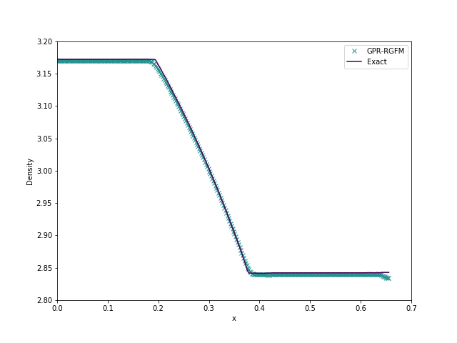
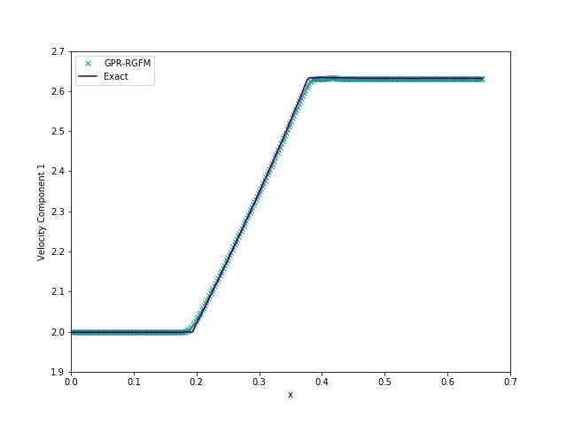
Refer to caption
Refer to caption
Refer to caption
Refer to caption
Refer to caption
Figure 10: Density, velocity, and total stress for the aluminium-vacuum test with GPR-RGFM, not including thermal conduction
Refer to caption
Refer to caption
Refer to caption
Figure 11: Density, velocity, and total stress for the aluminium-vacuum test with GPR-RGFM, including thermal conduction

3.5 Heat Conduction in a Gas

This test is based on the Heat Conduction in a Gas Test of Dumbser et al. [16]. Two ideal gases at different temperatures are initially in contact at position x=0𝑥0x=0. The initial conditions for this problem are given in Table 4 on page 4.


ρ𝜌\rho p𝑝p 𝒗𝒗\boldsymbol{v} A𝐴A 𝑱𝑱\boldsymbol{J}
x<0𝑥0x<0 222 111 𝟎0\boldsymbol{0} 23I332subscript𝐼3\sqrt[3]{2}\cdot I_{3} 𝟎0\boldsymbol{0}
x0𝑥0x\geq 0 0.50.50.5 111 𝟎0\boldsymbol{0} 123I3132subscript𝐼3\frac{1}{\sqrt[3]{2}}\cdot I_{3} 𝟎0\boldsymbol{0}
Table 4: Initial conditions for the heat conduction test

The material parameters are taken to be: γ=1.4𝛾1.4\gamma=1.4, cv=2.5subscript𝑐𝑣2.5c_{v}=2.5, ρ0=1subscript𝜌01\rho_{0}=1, p0=1subscript𝑝01p_{0}=1, cs=1subscript𝑐𝑠1c_{s}=1, ct=1subscript𝑐𝑡1c_{t}=1, μ=102𝜇superscript102\mu=10^{-2}, κ=102𝜅superscript102\kappa=10^{-2}. An interface is initially placed between the two volumes of air at x=0.5𝑥0.5x=0.5. The final time is taken to be t=1𝑡1t=1, and 200 cells are used. Results are displayed in Figure 12 on page 12, using the results from [16] as a reference. The material interface is denoted by a dashed vertical line.

The temperature curve generated using the GPR-RGFM matches very well the reference solution. The interface has moved to x=0.53756𝑥0.53756x=0.53756, as is to be expected, as the cooler gas on the left expands as it heats up, and the hotter gas on the right contracts as it cools. Initially, the mass of the left volume is 1 and the right volume is 0.25. At t=1𝑡1t=1, these masses are 0.9997 and 0.2503, respectively. Thus, mass on either side is conserved to a good approximation. Although the GPR-RGFM results for the heat flux match the reference solution well over most of the domain, there are aberrations in a small region around the interface. Although this doesn’t affect the temperature curve, these discrepancies are undesirable, and possible methods to rectify them are discussed in Section 4.
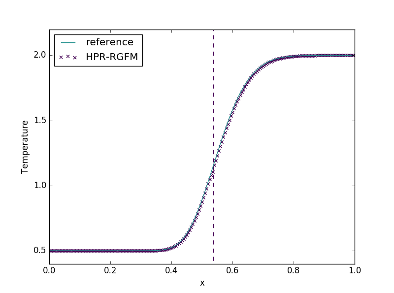
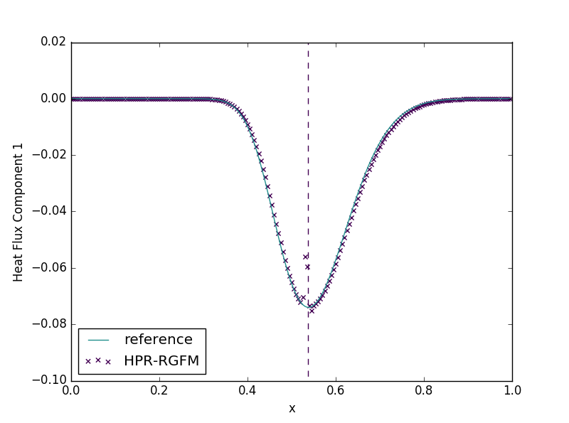
Refer to caption
Refer to caption
Refer to caption
Figure 12: Temperature, heat flux, and density for the intermaterial heat conduction test with GPR-RGFM

3.6 Taylor Bar

This follows a similar form to that found in [9, 39]. A bar of aluminium of dimensions 100×500100500100\times 500 travels towards a solid wall at speed 0.0150.0150.015. The surrounding environment is a vacuum. The aluminium bar is modelled by the shock Mie-Gruneisen equation of state, with parameters ρ0=2.785,subscript𝜌02.785\rho_{0}=2.785, cv=9×10⁴subscript𝑐𝑣9superscript104c_{v}=9\times 10^{-4}, c0=0.533subscript𝑐00.533c_{0}=0.533, Γ0=2subscriptΓ02\Gamma_{0}=2, s=1.338𝑠1.338s=1.338. The aluminium also follows a plasticity law with parameters b0=0.305subscript𝑏00.305b_{0}=0.305, σY=0.003subscript𝜎𝑌0.003\sigma_{Y}=0.003, τ0=1subscript𝜏01\tau_{0}=1, n=20𝑛20n=20. The domain has dimensions 300×510300510300\times 510, with Δx,Δy=1Δ𝑥Δ𝑦1\Delta x,\Delta y=1.

The density and plastic deformation of the bar at times t=0.0025𝑡0.0025t=0.0025 and t=0.005𝑡0.005t=0.005 are shown in Figure 13 on page 13. Unfortunately there are no experimental results for this test, but the reader is asked to note the good agreement here with the results found in [39]. In that study, the boundary between the bar and the vacuum is captured using a Lagrangian scheme, and it is reassuring that the same behaviour is captured here with a characteristically different numerical method.
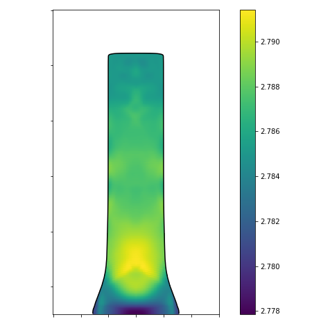
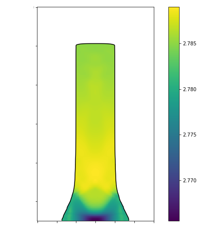
Refer to caption
Refer to caption
Refer to caption
Refer to caption
Figure 13: Density (top) and plastic deformation (bottom) for the Taylor bar test, at times t=0.0025𝑡0.0025t=0.0025 (left) and t=0.005𝑡0.005t=0.005 (right)

3.7 Aluminum Plate Impact

This test follows the form found in Michael & Nikiforakis [42] (based on the original formulation found in [31]). An aluminum projectile impacts upon an aluminum plate at speed 400400400. The domain is [0,0.03]×[0,0.04]00.0300.04\left[0,0.03\right]\times\left[0,0.04\right], with the projectile initially occupying [0.001,0.006]×[0.014,0.026]0.0010.0060.0140.026\left[0.001,0.006\right]\times\left[0.014,0.026\right], and the plate occupying [0.006,0.028]×[0.003,0.037]0.0060.0280.0030.037\left[0.006,0.028\right]\times\left[0.003,0.037\right]. We have Δx,Δy=104Δ𝑥Δ𝑦superscript104\Delta x,\Delta y=10^{-4}. The surroundings are taken to be a vacuum. The aluminium follows a Godunov-Romenski EOS with parameters ρ0=2710subscript𝜌02710\rho_{0}=2710, cv=900subscript𝑐𝑣900c_{v}=900, T0=300subscript𝑇0300T_{0}=300, c0=5037subscript𝑐05037c_{0}=5037, α=1𝛼1\alpha=1, β=3.577𝛽3.577\beta=3.577, γ=2.088𝛾2.088\gamma=2.088, b0=3160subscript𝑏03160b_{0}=3160, σY=4×10⁸subscript𝜎𝑌4superscript108\sigma_{Y}=4\times 10^{8}, τ0=1subscript𝜏01\tau_{0}=1, n=100𝑛100n=100. Gauges are placed initially at x=0.0078125𝑥0.0078125x=0.0078125, 0.01143750.01143750.0114375, 0.01506250.01506250.0150625, 0.01868750.01868750.0186875, 0.02231250.02231250.0223125 to measure the state variables over time, and these gauges are permitted to move with the local velocity of the material. The test is run until time t=5×10⁶𝑡5superscript106t=5\times 10^{-6}.

The pressure contours throughout the aluminium at various times are shown in Figure 14 on page 14. Despite relying on a slightly different plasticity model to that found in [42], it can be seen that these plots are in very good agreement with those found in the aforementioned publication. Note that release waves can be seen on the sides of the plate, in agreement with Michael & Nikiforakis.

Plots over time of the x𝑥x-velocity, pressure, density, and total stress - as measured by the gauges - are given in Figure 15 on page 15. Note the good agreement between these plots and those found in [42, 31], both in terms of their qualitative shape, and the arrival times of the waves that they represent. One can clearly see the separation between the elastic precursor wave and the trailing plastic wave in the impacted plate, and the subsequent return waves that are generated once these waves reach the end of the plate. This implies that the GPR-RGFM has correctly captured the aluminium-vacuum interface.
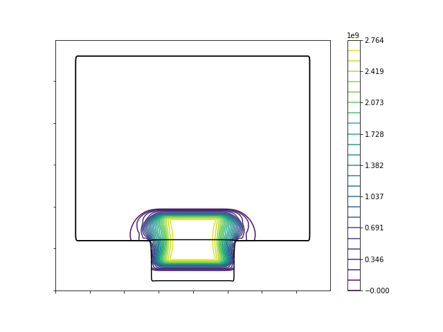
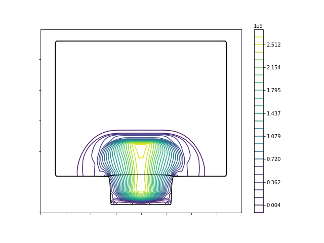
Refer to caption
Refer to caption
Refer to caption
Refer to caption
Figure 14: Pressure contour plots for the aluminium plate impact test, at times 0.5μs0.5𝜇𝑠0.5\mu s, 1μs1𝜇𝑠1\mu s, 3μs3𝜇𝑠3\mu s, 5μs5𝜇𝑠5\mu s
Refer to caption
Refer to caption
Refer to caption
Refer to caption
Figure 15: x𝑥x-velocity, pressure, density, and total stress over time, as measured by the various gauges of the aluminium plate impact test

3.8 Confined C4 Detonation without Backplate

This test is a variation of that found in [42]. A steel bar of length 0.03 and width 0.018 impacts upon a steel plate of depth 0.003, which is covering a region of depth 0.009 composed of C4 . The bar is initially traveling with speed 700. The system is surrounded by air.

The steel is modeled using a shock Mie-Gruneisen EOS, with parameters ρ0=7870subscript𝜌07870\rho_{0}=7870, cv=134subscript𝑐𝑣134c_{v}=134, c0=4569subscript𝑐04569c_{0}=4569, Γ0=2.17subscriptΓ02.17\Gamma_{0}=2.17, s=1.49𝑠1.49s=1.49, cs=3235subscript𝑐𝑠3235c_{s}=3235, σY=0.53×10⁹subscript𝜎𝑌0.53superscript109\sigma_{Y}=0.53\times 10^{9}, τ0=1subscript𝜏01\tau_{0}=1, n=10𝑛10n=10. The C4 is modeled using a JWL EOS, with parameters ρ0=1601subscript𝜌01601\rho_{0}=1601, cv=2.487×10⁶/1601subscript𝑐𝑣2.487superscript1061601c_{v}=2.487\times 10^{6}/1601, Γ0=0.8938subscriptΓ00.8938\Gamma_{0}=0.8938, A=7.781×10¹³𝐴7.781superscript1013A=7.781\times 10^{13}, B=5.031×10⁹𝐵5.031superscript109B=-5.031\times 10^{9}, R1=11.3subscript𝑅111.3R_{1}=11.3, R2=1.13subscript𝑅21.13R_{2}=1.13, cs=1487subscript𝑐𝑠1487c_{s}=1487. The air is modeled using an ideal gas EOS, with parameters ρ0=1.18subscript𝜌01.18\rho_{0}=1.18, cv=718subscript𝑐𝑣718c_{v}=718, γ=1.4𝛾1.4\gamma=1.4, cs=50subscript𝑐𝑠50c_{s}=50, μ=1.85×10⁵𝜇1.85superscript105\mu=1.85\times 10^{-5}.

The reaction of the C4 is captured using the ignition and growth model [34], where total energy E𝐸E is modified to include the term:

Er(λ)=Q(1λ)subscript𝐸𝑟𝜆𝑄1𝜆E_{r}\left(\lambda\right)=-Q\left(1-\lambda\right) (128)

with λ𝜆\lambda being the volume fraction of unreacted material, governed by the dynamical equation:

(ρλ)t+(ρλvk)xk=𝜌𝜆𝑡𝜌𝜆subscript𝑣𝑘subscript𝑥𝑘absent\displaystyle\frac{\partial\left(\rho\lambda\right)}{\partial t}+\frac{\partial\left(\rho\lambda v_{k}\right)}{\partial x_{k}}= ρK𝜌𝐾\displaystyle-\rho K (129a)
K=𝐾absent\displaystyle K= Iλb(ρρ01a)xH(ϕIϕ)𝐼superscript𝜆𝑏superscript𝜌subscript𝜌01𝑎𝑥𝐻subscriptitalic-ϕ𝐼italic-ϕ\displaystyle I\lambda^{b}\left(\frac{\rho}{\rho_{0}}-1-a\right)^{x}H\left(\phi_{I}-\phi\right) (129b)
+G1λcϕdpyH(ϕG1ϕ)subscript𝐺1superscript𝜆𝑐superscriptitalic-ϕ𝑑superscript𝑝𝑦𝐻subscriptitalic-ϕ𝐺1italic-ϕ\displaystyle+G_{1}\lambda^{c}\phi^{d}p^{y}H\left(\phi_{G1}-\phi\right)

In this test, the parameters are taken to be Q=9×10⁹/1601𝑄9superscript1091601Q=9\times 10^{9}/1601, I=4×10⁶𝐼4superscript106I=4\times 10^{6}, G1=1.4×10²⁰subscript𝐺11.4superscript1020G_{1}=1.4\times 10^{-20}, a=0.0367𝑎0.0367a=0.0367, b=2/3𝑏23b=2/3, c=2/3𝑐23c=2/3, d=1/3𝑑13d=1/3, x=7𝑥7x=7, y=2𝑦2y=2, ϕI=0.022subscriptitalic-ϕ𝐼0.022\phi_{I}=0.022, ϕG1=1subscriptitalic-ϕ𝐺11\phi_{G1}=1.

Figure 16 on page 16 displays the resulting pressure and C4 concentration at times t=2.4×10⁶𝑡2.4superscript106t=2.4\times 10^{-6} and t=4.9×10⁶𝑡4.9superscript106t=4.9\times 10^{-6}. As can be seen, the kinetic energy of the bar is correctly transmitted to the steel plate, with the plate deforming in a manner qualitatively identical to that found in [42]. This energy is in turn transmitted to the C4, leading to an exothermic reaction and a symmetrical wavefront that travels through the material. The C4 concentration is depleted to 0.93 at time t=2.4×10⁶𝑡2.4superscript106t=2.4\times 10^{-6} and to 0.915 at time t=4.9×10⁶𝑡4.9superscript106t=4.9\times 10^{-6}.

Refer to caption
Refer to caption
Refer to caption
Refer to caption
Figure 16: Pressure (left) and reactant concentration (right) for the confined detonation test (without back plate), at times 2.4μs2.4𝜇𝑠2.4\mu s (top) and 4.9μs4.9𝜇𝑠4.9\mu s (bottom)

3.9 Confined C4 Detonation

This test is identical to the previous test, except a steel plate of depth 0.003 is now placed behind the C4, so that the explosive is entirely confined. As can be seen from Figure 17 on page 17, the kinetic energy of the bar is once again correctly transmitted to the steel plate and C4, with the same deformation occurring in the first steel plate. At time t=2.4×10⁶𝑡2.4superscript106t=2.4\times 10^{-6} we see the wave in the C4 both partially rebounding off the backplate back into the reactant, and partially traveling on through the backplate. At the earlier time, the reactant concentration has been depleted to 0.88, and at the later time to 0.865. This corroborates the results of [42], in that the presence of the backplate accelerates the reactive processes.
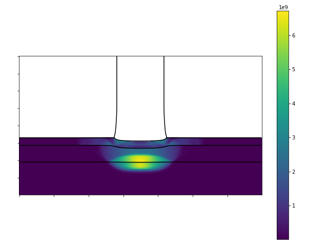
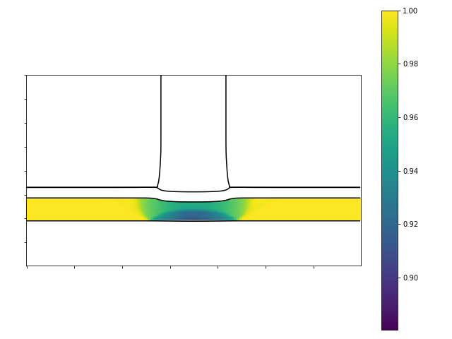
Refer to caption
Refer to caption
Refer to caption
Refer to caption
Figure 17: Pressure (left) and reactant concentration (right) for the confined detonation test, at times 2.4μs2.4𝜇𝑠2.4\mu s (top) and 4.9μs4.9𝜇𝑠4.9\mu s (bottom)

3.10 Confined C4 Detonation with Air Gap

This problem is designed to test the ability of the framework presented in this paper to capture the interaction of widely varying media. It is identical to the previous problem, except an air gap is now placed between the first steel plate and the C4. The air has the same EOS parameters as the surrounding air.

As can be seen in Figure 18 on page 18, the rod displaces the air (with the numerical method coping with contact of the region representing the plate with the region representing the C4). The displacement of the air enables the kinetic energy of the rod to be transmitted through the plate and into the C4, as before. The earlier time of t=2.4×10⁶𝑡2.4superscript106t=2.4\times 10^{-6} corresponds with the instant after the plate makes contact with the C4. The concentration is depleted to 0.9998 at t=2.4×10⁶𝑡2.4superscript106t=2.4\times 10^{-6} and 0.894 at t=4.9×10⁶𝑡4.9superscript106t=4.9\times 10^{-6}. The latter value is lower than the corresponding value in the previous test, as the reaction has been delayed by the presence of the air gap.
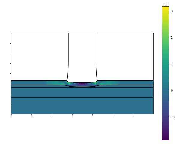
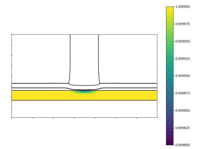
Refer to caption
Refer to caption
Refer to caption
Refer to caption
Figure 18: Pressure (left) and reactant concentration (right) for the confined detonation test (with air gap), at times 2.4μs2.4𝜇𝑠2.4\mu s (top) and 4.9μs4.9𝜇𝑠4.9\mu s (bottom)

3.11 Convergence Study

In order to determine the order of convergence of the Riemann Ghost Fluid Method presented in this study, the tests from 3.2, 3.3, and 3.4 were run with cell counts of 50,100,150,200,250,3005010015020025030050,100,150,200,250,300, and the error as compared with the exact solutions were calculated at the interfaces. The reason for choosing these two tests was to incorporate a range of different interface types (gas-liquid, fluid-solid, and solid-vacuum). The results are displayed in Table 5 on page 5. As can be seen, in all tests, the convergence rate is roughly first-order.


Water-Air Test PBX-Copper Test Aluminium-Vacuum Test
# Cells Error Rate Error Rate Error Rate
50 17.67419797 20.27348796 0.04232714
100 7.98596866 1.146 10.14165497 0.999 0.02180830 0.957
150 5.20404021 1.056 6.57517319 1.069 0.01365700 1.154
200 4.19411427 0.750 4.99100631 0.958 0.01005346 1.065
250 3.32431075 1.042 3.73732754 1.296 0.00793378 1.061
300 2.77425968 0.992 3.10851219 1.010 0.00571356 1.800
Table 5: Convergence Rates for the Water-Air Test, PBX-Copper Test, and Aluminium-Vacuum Test

4 Discussion

The Riemann Ghost Fluid Method presented in this study has been demonstrated to be an effective way of accurately simulating the interfaces between several different materials (in all three main phases of matter, plus vacuum), described by the GPR model. Unlike in many existing implementations, heat conduction across the interface was simulated accurately, leading to the representation of physical phenomena that are often overlooked, and to the redundancy of numerical techniques that are sometimes used to enforce more empirically-accurate results (such as entropy and temperature fixes).

The framework presented here greatly simplifies the conceptual framework required for multimaterial interactions. Implementation should be easier and quicker, and future work can be more focused on a single model, rather than several fundamentally different frameworks.

4.1 Limitations

Throughout this study, the various fluids have been assumed to be immiscible. Whilst this is a common assumption in situations where mixing is low or practically non-existent, there are many problems which may require it. An area of further research would be the implementation of a mixture model such as that proposed by Romenski et al. [55, 54], which uses the same thermal conduction system as the GPR model.

The truncation of the Taylor series expansions (98a) and (98b) used to find the star states of the heat flux and the viscous stress tensor implicitly assumes that there are only small differences between the side states and the star states of the variables upon which q1,𝝈𝟏superscriptsubscript𝑞1superscriptsubscript𝝈1q_{1}^{*},\boldsymbol{\sigma_{1}^{*}} depend (ρ𝜌\rho, p𝑝p, J1subscript𝐽1J_{1}, and 𝑨𝟏subscript𝑨1\boldsymbol{A_{1}}). If this is the case, higher order terms of the expansion can be neglected. If it is not, however, the method may fail. The linearised nature of the GPR-RGFM solver also implicitly assumes that all waves of interest present in the Riemann Problem are shocks. Thus, strong rarefactions may cause the method to fail.

4.2 Potential Improvements

As noted in Section 3.5, the GPR-RGFM method does not necessarily ensure the continuity of the normal component of heat flux across interfaces that feature discontinuous temperature jumps. This is despite the method accurately modeling both the heat conduction across the interface over time, and the corresponding evolution to thermal equilibrium between the two materials. The reason for this is that the star states produced by the linearised solver presented in Section 2.2 represent the state of the system at a time slightly beyond the point in time at which they are applied to neighboring ghost cells. With more simple systems of PDEs - such as the Euler equations - this often doesn’t matter, as the star states are constant in time, or their time evolution is easily calculated. Owing to the source terms in the GPR equations, however, the star states evolve in a manner for which an analytical solution is not available. Thus, when the star states are applied to the ghost cells, they contain higher heat fluxes and slightly different temperatures to the actual values at the interface at that moment in time, leading to the slight aberration apparent in the heat flux in Figure 12 on page 12.

A possible solution to this is as follows: Take materials L𝐿L and R𝑅R either side of an interface. Given the states straddling the interface, QL,QRsubscript𝑄𝐿subscript𝑄𝑅Q_{L},Q_{R}, derive QLsuperscriptsubscript𝑄𝐿Q_{L}^{*} using the procedure outlined in Section 2.2. Then, by inverting this procedure, derive a state QR~~subscript𝑄𝑅\tilde{Q_{R}} such that if QL,QR~subscript𝑄𝐿~subscript𝑄𝑅Q_{L},\tilde{Q_{R}} are both states for material L𝐿L (rather than for materials L𝐿L and R𝑅R, respectively), following the procedure in Section 2.2 obtains the same star state, QLsuperscriptsubscript𝑄𝐿Q_{L}^{*}. The derivation of such an inverse mapping should be feasible, possibly with the addition of some physical constraints. In this way, QR~~subscript𝑄𝑅\tilde{Q_{R}} represents a state for the righthand cell at the current time, which - if cell R𝑅R were occupied by material L𝐿L - would result in the same state on the lefthand side of the interface at the end of the current timestep as if the righthand cell were occupied by QRsubscript𝑄𝑅Q_{R} and material R𝑅R.

Another clear improvement to the GPR-RGFM method presented would be to use a better Riemann solver than the iterative, linearised solver devised in Section 2.2. Let L𝐿L be the matrix of left eigenvectors of the primitive system. As noted previously, the solver relies upon the fact that each of the following relations holds along the characteristic to which it corresponds:

Ld𝑷dt=L𝑺𝐿𝑑𝑷𝑑𝑡𝐿𝑺L\cdot\frac{d\boldsymbol{P}}{dt}=L\cdot\boldsymbol{S} (130)

Methods to accurately integrate (130) from the left and right interface boundary states to their respective star states warrant further research.

Alternatively, a completely different approximate Riemann solver could be employed, such as the universal HLLEM solver of Dumbser et al. [15]. This path-conservative formulation of the HLLEM solver works for general non-conservative systems (such as the GPR model) and is simple to implement. It’s based upon a new path-conservative HLL method (building on the original method of Harten, Lax, and van Leer [27]) but is claimed to be able to represent linearly degenerate intermediate waves “with a minimum of smearing” by evaluating the eigenvalues and eigenvectors of the intermediate characteristic fields (given in Section 2.1).

There are iterative exact Riemann solvers for the equations of non-linear elasticity (to which the GPR model reduces as τ1subscript𝜏1\tau_{1}\rightarrow\infty). Thus, they will work for applications of the GPR model to solids problems (and perhaps to very viscous fluids problems too). Although these solvers are computationally expensive, they are only used once at each material interface point at each time step, and thus the added accuracy that they provide may be desirable. There are two ways to formulate the equations of non-linear elasticity: one in which the deformation tensor (the analogue of the inverse of the GPR model’s distortion tensor) is evolved in time, and one in which its inverse (the analogue of A𝐴A) is evolved instead. Miller’s exact solver [43] uses the first formulation and the solver of Barton et al. [5] uses the second. The former can be used to evolve A1superscript𝐴1A^{-1}, from which A𝐴A can be calculated. Unfortunately, both solvers critically assume that the source terms of the system vanish, and so are unlikely to produce the correct boundary conditions for the GPR-RGFM when modeling relatively inviscid fluids. It should also be noted that they cannot be used for problems involving heat conduction across material interfaces, and they do not take the thermal conduction subsystem of the GPR model into account.

5 References

References

  • [1] F. Alcrudo and F. Benkhaldoun, Exact solutions to the Riemann problem of the shallow water equations with a bottom step, Computers & Fluids, 30 (2001), pp. 643–671.
  • [2] P. T. Barton and D. Drikakis, An Eulerian method for multi-component problems in non-linear elasticity with sliding interfaces, Journal of Computational Physics, 229 (2010), pp. 5518–5540.
  • [3] P. T. Barton and D. Drikakis, An Eulerian method for multi-component problems in non-linear elasticity with sliding interfaces, Journal of Computational Physics, 229 (2010), pp. 5518–5540.
  • [4] P. T. Barton, D. Drikakis, E. Romenski, and V. a. Titarev, Exact and approximate solutions of Riemann problems in non-linear elasticity, Journal of Computational Physics, 228 (2009), pp. 7046–7068.
  • [5]  , Exact and approximate solutions of Riemann problems in non-linear elasticity, Journal of Computational Physics, 228 (2009), pp. 7046–7068.
  • [6] P. T. Barton, D. Drikakis, and E. I. Romenski, An Eulerian finite-volume scheme for large elastoplastic deformations in solids, International Journal for Numerical Methods in Engineering, 81 (2011), pp. 453–484.
  • [7] P. T. Barton, B. Obadia, and D. Drikakis, A conservative level-set based method for compressible solid/fluid problems on fixed grids, Journal of Computational Physics, 230 (2011), pp. 7867–7890.
  • [8] J. Boettger, K. G. Honnell, J. H. Peterson, C. Greeff, and S. Crockett, Tabular equation of state for gold, AIP Conference Proceedings, 1426 (2012), pp. 812–815.
  • [9] W. Boscheri, M. Dumbser, and R. Loubere, Cell centered direct Arbitrary-Lagrangian-Eulerian ADER-WENO finite volume schemes for nonlinear hyperelasticity, Computers and Fluids, 134-135 (2016), pp. 111–129.
  • [10] A. d. Brauer, A. Iollo, and T. Milcent, A Cartesian Scheme for Compressible Multimaterial Hyperelastic Models with Plasticity, Communications in Computational Physics, 22 (2017), pp. 1362–1384.
  • [11] N. Buyukcizmeci, A. S. Botvina, and I. N. Mishustin, Tabulated Equation of State for Supernova Matter Including Full Nuclear Ensemble, The Astrophysical Journal, 789 (2014), p. 33.
  • [12] A. Chinnayya, E. Daniel, and R. Saurel, Modelling detonation waves in heterogeneous energetic materials, Journal of Computational Physics, 196 (2004), pp. 490–538.
  • [13] A. de Brauer, A. Iollo, and T. Milcent, A Cartesian scheme for compressible multimaterial models in 3d, Journal of Computational Physics, 313 (2016), pp. 121–143.
  • [14] J. Donea, S. Giuliani, and J. P. Halleux, An arbitrary lagrangian-eulerian finite element method for transient dynamic fluid-structure interactions, Computer Methods in Applied Mechanics and Engineering, 33 (1982), pp. 689–723.
  • [15] M. Dumbser and D. S. Balsara, A new efficient formulation of the HLLEM Riemann solver for general conservative and non-conservative hyperbolic systems, Journal of Computational Physics, 304 (2016), pp. 275–319.
  • [16] M. Dumbser, I. Peshkov, E. Romenski, and O. Zanotti, High order ADER schemes for a unified first order hyperbolic formulation of continuum mechanics: viscous heat-conducting fluids and elastic solids, Journal of Computational Physics, 314 (2015), pp. 824–862.
  • [17] M. Dumbser and E. F. Toro, On universal Osher-type schemes for general nonlinear hyperbolic conservation laws, Communications in Computational Physics, 10 (2011), pp. 635–671.
  • [18] M. Dumbser and E. F. Toro, A simple extension of the Osher Riemann solver to non-conservative hyperbolic systems, Journal of Scientific Computing, 48 (2011), pp. 70–88.
  • [19] M. Dumbser, O. Zanotti, A. Hidalgo, and D. S. Balsara, ADER-WENO finite volume schemes with space-time adaptive mesh refinement, Journal of Computational Physics, 248 (2013), pp. 257–286.
  • [20] N. Favrie and S. L. Gavrilyuk, Diffuse interface model for compressible fluid - Compressible elastic-plastic solid interaction, Journal of Computational Physics, 231 (2012), pp. 2695–2723.
  • [21] N. Favrie, S. L. Gavrilyuk, and R. Saurel, Solid-fluid diffuse interface model in cases of extreme deformations, Journal of Computational Physics, 228 (2009), pp. 6037–6077.
  • [22] R. Fedkiw, T. Aslam, B. Merriman, and S. Osher, A Non-oscillatory Eulerian Approach to Interfaces in Multimaterial Flows (the Ghost Fluid Method), Journal of Computational Physics, 152 (1999), pp. 457–492.
  • [23]  , A Non-oscillatory Eulerian Approach to Interfaces in Multimaterial Flows (the Ghost Fluid Method), Journal of Computational Physics, 152 (1999), pp. 457–492.
  • [24] R. P. Fedkiw, Coupling an Eulerian Fluid Calculation to a Lagrangian Solid Calculation with the Ghost Fluid Method, Journal of Computational Physics, 175 (2002), pp. 200–224.
  • [25] J. Frenkel, Kinetic Theory of Liquids, Oxford University Press, 1947.
  • [26] J. Glimm and D. Marchesin, A Numerical Method for Two Phase Flow with an Unstable Interface, Journal of Computational Physics, 39 (1981), pp. 179–200.
  • [27] A. Harten, P. D. Lax, and B. van Leer, On Upstream Differencing and Godunov-Type Schemes for Hyperbolic Conservation Laws, SIAM Review, 25 (1983), pp. 35–61.
  • [28] F. Hempert, S. Boblest, T. Ertl, F. Sadlo, P. Offenhauser, C. W. Glass, M. Hoffmann, A. Beck, C. D. Munz, and U. Iben, Simulation of real gas effects in supersonic methane jets using a tabulated equation of state with a discontinuous Galerkin spectral element method, Computers & Fluids, 145 (2017), pp. 167–179.
  • [29] C. W. Hirt and B. D. Nichols, Volume of fluid (VOF) method for the dynamics of free boundaries, Journal of Computational Physics, 39 (1981), pp. 201–225.
  • [30] G. Hou, J. Wang, and A. Layton, Numerical methods for fluid-structure interaction - A review, Communications in Computational Physics, 12 (2012), pp. 337–377.
  • [31] B. Howell and G. Ball, A Free Lagrange Augmented Godunov Method for the Simulation of Elastic Plastic Solids, Journal of Computational Physics, 175 (2002), pp. 128–167.
  • [32] H. Jackson, A Fast Numerical Scheme for the Godunov-Peshkov-Romenski Model of Continuum Mechanics, Journal of Computational Physics, 348 (2017), pp. 514–533.
  • [33] H. Jackson and N. Nikiforakis, A numerical scheme for non-Newtonian fluids and plastic solids under the GPR model, Journal of Computational Physics, 387 (2019), pp. 410–429.
  • [34] E. L. Lee and C. M. Tarver, Phenomenological model of shock initiation in heterogeneous explosives, Physics of Fluids, 23 (1980), p. 2362.
  • [35] A. Legay, J. Chessa, and T. Belytschko, An Eulerian-Lagrangian method for fluid-structure interaction based on level sets, Computer Methods in Applied Mechanics & Engineering, 195 (2006), pp. 2070–2087.
  • [36] P. R. Levashov and K. V. Khishchenko, Tabular multiphase equations of state for metals and their applications, AIP Conference Proceedings, 955 (2007), pp. 59–62.
  • [37] T. G. Liu, B. C. Khoo, and K. S. Yeo, Ghost fluid method for strong shock impacting on material interface, Journal of Computational Physics, 190 (2003), pp. 651–681.
  • [38] T.-P. Liu, The Riemann problem for general systems of conservation laws, Journal of Differential Equations, 18 (1975), pp. 218–234.
  • [39] P. H. Maire, R. Abgrall, J. Breil, R. Loubere, and B. Rebourcet, A nominally second-order cell-centered Lagrangian scheme for simulating elastic-plastic flows on two-dimensional unstructured grids, Journal of Computational Physics, 235 (2013), pp. 626–665.
  • [40] A. N. Malyshev and E. I. Romenskii, Hyperbolic equations for heat transfer. Global solvability of the Cauchy problem, Siberian Mathematical Journal, 27 (1986), pp. 734–740.
  • [41] L. Michael and N. Nikiforakis, Coupling of elastoplastic solid models with condensed-phase explosives formulations, (submitted), (2016).
  • [42] L. Michael and N. Nikiforakis, A multi-physics methodology for the simulation of reactive flow and elastoplastic structural response, Journal of Computational Physics, 367 (2018), pp. 1–27.
  • [43] G. H. Miller, An iterative Riemann solver for systems of hyperbolic conservation laws, with application to hyperelastic solid mechanics, Journal of Computational Physics, 193 (2004), pp. 198–225.
  • [44] S. Ndanou, N. Favrie, and S. Gavrilyuk, Multi-solid and multi-fluid diffuse interface model: Applications to dynamic fracture and fragmentation, Journal of Computational Physics, 295 (2015), pp. 523–555.
  • [45] B. D. Nichols, C. W. Hirt, and R. S. Hotchkiss, SOLA-VOF: A solution algorithm for transient fluid flow with multiple free boundaries, NASA STI/Recon Technical Report N, 81 (1980).
  • [46] S. Osher and R. Fedkiw, Level Set Methods and Dynamic Implicit Surfaces, Springer, 2002.
  • [47] S. Osher and R. P. Fedkiw, Level Set Methods: An Overview and Some Recent Results, Journal of Computational Physics, 169 (2001), pp. 463–502.
  • [48] I. Peshkov, W. Boscheri, R. LoubÚre, E. Romenski, and M. Dumbser, Theoretical and numerical comparison of hyperelastic and hypoelastic formulations for Eulerian non-linear elastoplasticity, Journal of Computational Physics, 387 (2019), pp. 481–521.
  • [49] I. Peshkov and E. Romenski, A hyperbolic model for viscous Newtonian flows, Continuum Mechanics and Thermodynamics, 28 (2016), pp. 85–104.
  • [50] J. H. Peterson, K. G. Honnell, C. Greeff, J. D. Johnson, J. Boettger, and S. Crockett, Global equation of state for copper, Chicago, Illinois, 2012, pp. 763–766.
  • [51] F. D. Pin, S. Idelsohn, E. Onate, and R. Aubry, The ALE/Lagrangian Particle Finite Element Method: A new approach to computation of free-surface flows and fluid-object interactions, Computers & Fluids, 36 (2007), pp. 27–38.
  • [52] W. J. Rider and D. B. Kothe, Reconstructing Volume Tracking, Journal of Computational Physics, 141 (1998), pp. 112–152.
  • [53] E. Romenski, D. Drikakis, and E. Toro, Conservative models and numerical methods for compressible two-phase flow, Journal of Scientific Computing, 42 (2010), pp. 68–95.
  • [54]  , Conservative models and numerical methods for compressible two-phase flow, Journal of Scientific Computing, 42 (2010), pp. 68–95.
  • [55] E. Romenski, A. D. Resnyansky, and E. F. Toro, Conservative Hyperbolic Formulation for Compressible Two-Phase Flow with Different Phase Pressures and Temperatures, Quarterly of Applied Mathematics, 65 (2007), pp. 259–279.
  • [56] E. Romenski, A. D. Resnyansky, and E. F. Toro, Conservative hyperbolic model for compressible two-phase flow with different phase pressures and temperatures, Quarterly of applied mathematics, 65(2) (2007), pp. 259–279.
  • [57] E. I. Romenski, Hyperbolic equations of Maxwell’s nonlinear model of elastoplastic heat-conducting media, Siberian Mathematical Journal, 30 (1989), pp. 606–625.
  • [58] P. B. Ryzhakov, R. Rossi, S. R. Idelsohn, and E. Onate, A monolithic Lagrangian approach for fluid-structure interaction problems, Computational Mechanics, 46 (2010), pp. 883–899.
  • [59] S. K. Sambasivan and H. S. UdayKumar, Ghost Fluid Method for Strong Shock Interactions Part 1: Fluid-Fluid Interfaces, AIAA Journal, 47 (2009), pp. 2907–2922.
  • [60]  , Ghost Fluid Method for Strong Shock Interactions Part 2: Immersed Solid Boundaries, AIAA Journal, 47 (2009), pp. 2923–2937.
  • [61] R. Saurel and R. Abgrall, A Multiphase Godunov Method for Compressible Multifluid and Multiphase Flows, Journal of Computational Physics, 150 (1999), pp. 425–467.
  • [62] R. Scardovelli and S. Zaleski, Direct numerical simulation of free-surface and interfacial flow, Annual Review of Fluid Mechanics, 31 (1999), pp. 567–603.
  • [63] S. Schoch, K. Nordin-Bates, and N. Nikiforakis, An Eulerian algorithm for coupled simulations of elastoplastic-solids and condensed-phase explosives, Journal of Computational Physics, 252 (2013), pp. 163–194.
  • [64] E. F. Toro, Reimann Solvers and Numerical Methods for fluid dynamics, vol. 40, 2009.
  • [65] E. F. Toro, Riemann Solvers and Numerical Methods for Fluid Dynamics: A Practical Introduction, Springer, 2009.
  • [66] S. P. Wang, M. H. Anderson, J. G. Oakley, M. L. Corradini, and R. Bonazza, A thermodynamically consistent and fully conservative treatment of contact discontinuities for compressible multicomponent flows, Journal of Computational Physics, 195 (2004), pp. 528–559.

6 Acknowledgments

The authors acknowledge financial support from the EPSRC Centre for Doctoral Training in Computational Methods for Materials Science under grant EP/L015552/1.

7 Appendix

Taking the ordering 𝑷𝑷\boldsymbol{P} of primitive variables in (144), note that (1e), (1b), (1c), (1d) can be stated as:

DρDt+ρvkxk𝐷𝜌𝐷𝑡𝜌subscript𝑣𝑘subscript𝑥𝑘\displaystyle\frac{D\rho}{Dt}+\rho\frac{\partial v_{k}}{\partial x_{k}} =0absent0\displaystyle=0 (131a)
DviDt+1ρΣikxk𝐷subscript𝑣𝑖𝐷𝑡1𝜌subscriptΣ𝑖𝑘subscript𝑥𝑘\displaystyle\frac{Dv_{i}}{Dt}+\frac{1}{\rho}\frac{\partial\Sigma_{ik}}{\partial x_{k}} =0absent0\displaystyle=0 (131b)
DAijDt+Aikvkxj𝐷subscript𝐴𝑖𝑗𝐷𝑡subscript𝐴𝑖𝑘subscript𝑣𝑘subscript𝑥𝑗\displaystyle\frac{DA_{ij}}{Dt}+A_{ik}\frac{\partial v_{k}}{\partial x_{j}} =ψijθ1absentsubscript𝜓𝑖𝑗subscript𝜃1\displaystyle=-\frac{\psi_{ij}}{\theta_{1}} (131c)
DJiDt+1ρTδikxk𝐷subscript𝐽𝑖𝐷𝑡1𝜌𝑇subscript𝛿𝑖𝑘subscript𝑥𝑘\displaystyle\frac{DJ_{i}}{Dt}+\frac{1}{\rho}\frac{\partial T\delta_{ik}}{\partial x_{k}} =Hiθ2absentsubscript𝐻𝑖subscript𝜃2\displaystyle=-\frac{H_{i}}{\theta_{2}} (131d)
DEDt+1ρ(Σikvi+THk)xk𝐷𝐸𝐷𝑡1𝜌subscriptΣ𝑖𝑘subscript𝑣𝑖𝑇subscript𝐻𝑘subscript𝑥𝑘\displaystyle\frac{DE}{Dt}+\frac{1}{\rho}\frac{\partial\left(\Sigma_{ik}v_{i}+TH_{k}\right)}{\partial x_{k}} =0absent0\displaystyle=0 (131e)

where the total stress tensor Σ=pI+ρATψΣ𝑝𝐼𝜌superscript𝐴𝑇𝜓\Sigma=pI+\rho A^{T}\psi. Note that:

DEDt𝐷𝐸𝐷𝑡\displaystyle\frac{DE}{Dt} =EpDpDt+EρDρDt+viDviDt+EAijDAijDt+HiDJiDtabsent𝐸𝑝𝐷𝑝𝐷𝑡𝐸𝜌𝐷𝜌𝐷𝑡subscript𝑣𝑖𝐷subscript𝑣𝑖𝐷𝑡𝐸subscript𝐴𝑖𝑗𝐷subscript𝐴𝑖𝑗𝐷𝑡subscript𝐻𝑖𝐷subscript𝐽𝑖𝐷𝑡\displaystyle=\frac{\partial E}{\partial p}\frac{Dp}{Dt}+\frac{\partial E}{\partial\rho}\frac{D\rho}{Dt}+v_{i}\frac{Dv_{i}}{Dt}+\frac{\partial E}{\partial A_{ij}}\frac{DA_{ij}}{Dt}+H_{i}\frac{DJ_{i}}{Dt} (132)
=EpDpDtρEρvkxk1ρviΣikxkEAij(Aikvkxj+ψijθ1)Hi(1ρTδikxk+Hiθ2)absent𝐸𝑝𝐷𝑝𝐷𝑡𝜌𝐸𝜌subscript𝑣𝑘subscript𝑥𝑘1𝜌subscript𝑣𝑖subscriptΣ𝑖𝑘subscript𝑥𝑘𝐸subscript𝐴𝑖𝑗subscript𝐴𝑖𝑘subscript𝑣𝑘subscript𝑥𝑗subscript𝜓𝑖𝑗subscript𝜃1subscript𝐻𝑖1𝜌𝑇subscript𝛿𝑖𝑘subscript𝑥𝑘subscript𝐻𝑖subscript𝜃2\displaystyle=\frac{\partial E}{\partial p}\frac{Dp}{Dt}-\rho\frac{\partial E}{\partial\rho}\frac{\partial v_{k}}{\partial x_{k}}-\frac{1}{\rho}v_{i}\frac{\partial\Sigma_{ik}}{\partial x_{k}}-\frac{\partial E}{\partial A_{ij}}\left(A_{ik}\frac{\partial v_{k}}{\partial x_{j}}+\frac{\psi_{ij}}{\theta_{1}}\right)-H_{i}\left(\frac{1}{\rho}\frac{\partial T\delta_{ik}}{\partial x_{k}}+\frac{H_{i}}{\theta_{2}}\right)

Thus, the energy equation becomes:

EpDpDtρEρvkxk1ρviΣikxkEAijAikvkxjHkρTxk+1ρ(Σikvi+THk)xk=EAijψijθ1+HiHiθ2𝐸𝑝𝐷𝑝𝐷𝑡𝜌𝐸𝜌subscript𝑣𝑘subscript𝑥𝑘1𝜌subscript𝑣𝑖subscriptΣ𝑖𝑘subscript𝑥𝑘𝐸subscript𝐴𝑖𝑗subscript𝐴𝑖𝑘subscript𝑣𝑘subscript𝑥𝑗subscript𝐻𝑘𝜌𝑇subscript𝑥𝑘1𝜌subscriptΣ𝑖𝑘subscript𝑣𝑖𝑇subscript𝐻𝑘subscript𝑥𝑘𝐸subscript𝐴𝑖𝑗subscript𝜓𝑖𝑗subscript𝜃1subscript𝐻𝑖subscript𝐻𝑖subscript𝜃2\frac{\partial E}{\partial p}\frac{Dp}{Dt}-\rho\frac{\partial E}{\partial\rho}\frac{\partial v_{k}}{\partial x_{k}}-\frac{1}{\rho}v_{i}\frac{\partial\Sigma_{ik}}{\partial x_{k}}-\frac{\partial E}{\partial A_{ij}}A_{ik}\frac{\partial v_{k}}{\partial x_{j}}-\frac{H_{k}}{\rho}\frac{\partial T}{\partial x_{k}}+\frac{1}{\rho}\frac{\partial\left(\Sigma_{ik}v_{i}+TH_{k}\right)}{\partial x_{k}}=\frac{\partial E}{\partial A_{ij}}\frac{\psi_{ij}}{\theta_{1}}+\frac{H_{i}H_{i}}{\theta_{2}} (133)

Simplifying:

DpDt+1ρEp(ΣikρAjiEAjkρ2Eρδik)vixk+TρEpHkxk=EAijψijθ1Ep+HiHiθ2Ep𝐷𝑝𝐷𝑡1𝜌subscript𝐸𝑝subscriptΣ𝑖𝑘𝜌subscript𝐴𝑗𝑖𝐸subscript𝐴𝑗𝑘superscript𝜌2𝐸𝜌subscript𝛿𝑖𝑘subscript𝑣𝑖subscript𝑥𝑘𝑇𝜌subscript𝐸𝑝subscript𝐻𝑘subscript𝑥𝑘𝐸subscript𝐴𝑖𝑗subscript𝜓𝑖𝑗subscript𝜃1subscript𝐸𝑝subscript𝐻𝑖subscript𝐻𝑖subscript𝜃2subscript𝐸𝑝\frac{Dp}{Dt}+\frac{1}{\rho E_{p}}\left(\Sigma_{ik}-\rho A_{ji}\frac{\partial E}{\partial A_{jk}}-\rho^{2}\frac{\partial E}{\partial\rho}\delta_{ik}\right)\frac{\partial v_{i}}{\partial x_{k}}+\frac{T}{\rho E_{p}}\frac{\partial H_{k}}{\partial x_{k}}=\frac{\partial E}{\partial A_{ij}}\frac{\psi_{ij}}{\theta_{1}E_{p}}+\frac{H_{i}H_{i}}{\theta_{2}E_{p}} (134)

We have666 pρ2EρρEp𝑝superscript𝜌2subscript𝐸𝜌𝜌subscript𝐸𝑝\displaystyle\frac{p-\rho^{2}E_{\rho}}{\rho E_{p}} =ρ2Eρ|sρ2Eρ|pρEp|ρ=ρEρ|s(Eρ|s+Es|ρsρ|p)Es|ρsp|ρabsentevaluated-atsuperscript𝜌2subscript𝐸𝜌𝑠evaluated-atsuperscript𝜌2subscript𝐸𝜌𝑝evaluated-at𝜌subscript𝐸𝑝𝜌𝜌evaluated-atsubscript𝐸𝜌𝑠evaluated-atsubscript𝐸𝜌𝑠evaluated-atevaluated-atsubscript𝐸𝑠𝜌subscript𝑠𝜌𝑝evaluated-atevaluated-atsubscript𝐸𝑠𝜌subscript𝑠𝑝𝜌\displaystyle=\frac{\rho^{2}\left.E_{\rho}\right|_{s}-\rho^{2}\left.E_{\rho}\right|_{p}}{\rho\left.E_{p}\right|_{\rho}}=\rho\frac{\left.E_{\rho}\right|_{s}-\left(\left.E_{\rho}\right|_{s}+\left.E_{s}\right|_{\rho}\left.s_{\rho}\right|_{p}\right)}{\left.E_{s}\right|_{\rho}\left.s_{p}\right|_{\rho}} (135) =ρsρ|psp|ρ=ρpρ|sabsent𝜌evaluated-atsubscript𝑠𝜌𝑝evaluated-atsubscript𝑠𝑝𝜌evaluated-at𝜌𝑝𝜌𝑠\displaystyle=\rho\frac{-\left.s_{\rho}\right|_{p}}{\left.s_{p}\right|_{\rho}}=\rho\left.\frac{\partial p}{\partial\rho}\right|_{s} 777 ct2TρEp=ct2TρcvTp=ρch2Tpsuperscriptsubscript𝑐𝑡2𝑇𝜌subscript𝐸𝑝superscriptsubscript𝑐𝑡2𝑇𝜌subscript𝑐𝑣subscript𝑇𝑝𝜌superscriptsubscript𝑐2subscript𝑇𝑝\frac{c_{t}^{2}T}{\rho E_{p}}=\frac{c_{t}^{2}T}{\rho c_{v}T_{p}}=\frac{\rho c_{h}^{2}}{T_{p}} (136) 888 EA|ρ,p=(cs2ρΓcs2ρ)ψcs2=(12ρ2ρΓlog(cs)ρ)ψevaluated-at𝐸𝐴𝜌𝑝superscriptsubscript𝑐𝑠2𝜌Γsuperscriptsubscript𝑐𝑠2𝜌𝜓superscriptsubscript𝑐𝑠212superscript𝜌2𝜌Γsubscript𝑐𝑠𝜌𝜓\left.\frac{\partial E}{\partial A}\right|_{\rho,p}=\left(c_{s}^{2}-\frac{\rho}{\Gamma}\frac{\partial c_{s}^{2}}{\partial\rho}\right)\frac{\psi}{c_{s}^{2}}=\left(1-2\frac{\rho^{2}}{\rho\Gamma}\frac{\partial\log\left(c_{s}\right)}{\partial\rho}\right)\psi (137) σρ𝜎𝜌\displaystyle\frac{\partial\sigma}{\partial\rho} =ρ(ρcs2ATψcs2)=cs2ATψcs2ρcs2ρATψcs2absent𝜌𝜌superscriptsubscript𝑐𝑠2superscript𝐴𝑇𝜓superscriptsubscript𝑐𝑠2superscriptsubscript𝑐𝑠2superscript𝐴𝑇𝜓superscriptsubscript𝑐𝑠2𝜌superscriptsubscript𝑐𝑠2𝜌superscript𝐴𝑇𝜓superscriptsubscript𝑐𝑠2\displaystyle=\frac{\partial}{\partial\rho}\left(-\rho c_{s}^{2}A^{T}\frac{\psi}{c_{s}^{2}}\right)=-c_{s}^{2}A^{T}\frac{\psi}{c_{s}^{2}}-\rho\frac{\partial c_{s}^{2}}{\partial\rho}A^{T}\frac{\psi}{c_{s}^{2}} (138) =σρ+2log(cs)ρσabsent𝜎𝜌2subscript𝑐𝑠𝜌𝜎\displaystyle=\frac{\sigma}{\rho}+2\frac{\partial\log\left(c_{s}\right)}{\partial\rho}\sigma :

pρ2EρρEp𝑝superscript𝜌2subscript𝐸𝜌𝜌subscript𝐸𝑝\displaystyle\frac{p-\rho^{2}E_{\rho}}{\rho E_{p}} =ρc02absent𝜌superscriptsubscript𝑐02\displaystyle=\rho c_{0}^{2} (139a)
ct2TρEpsuperscriptsubscript𝑐𝑡2𝑇𝜌subscript𝐸𝑝\displaystyle\frac{c_{t}^{2}T}{\rho E_{p}} =ρch2Tpabsent𝜌superscriptsubscript𝑐2subscript𝑇𝑝\displaystyle=\frac{\rho c_{h}^{2}}{T_{p}} (139b)
EA|ρ,pevaluated-at𝐸𝐴𝜌𝑝\displaystyle\left.\frac{\partial E}{\partial A}\right|_{\rho,p} =(12ρ2Eplog(cs)ρ)ψabsent12superscript𝜌2subscript𝐸𝑝subscript𝑐𝑠𝜌𝜓\displaystyle=\left(1-2\rho^{2}E_{p}\frac{\partial\log\left(c_{s}\right)}{\partial\rho}\right)\psi (139c)
ρATEA|ρ,pevaluated-at𝜌superscript𝐴𝑇𝐸𝐴𝜌𝑝\displaystyle-\rho A^{T}\left.\frac{\partial E}{\partial A}\right|_{\rho,p} =σ+ρ2Ep(σρσρ)absent𝜎superscript𝜌2subscript𝐸𝑝𝜎𝜌𝜎𝜌\displaystyle=\sigma+\rho^{2}E_{p}\left(\frac{\sigma}{\rho}-\frac{\partial\sigma}{\partial\rho}\right) (139d)

The full system then becomes:

DρDt+ρvkxk𝐷𝜌𝐷𝑡𝜌subscript𝑣𝑘subscript𝑥𝑘\displaystyle\frac{D\rho}{Dt}+\rho\frac{\partial v_{k}}{\partial x_{k}} =0absent0\displaystyle=0 (140a)
DpDt+ρc02vixi+(σikρσikρ)vixk+ρch2TpJkxk𝐷𝑝𝐷𝑡𝜌superscriptsubscript𝑐02subscript𝑣𝑖subscript𝑥𝑖subscript𝜎𝑖𝑘𝜌subscript𝜎𝑖𝑘𝜌subscript𝑣𝑖subscript𝑥𝑘𝜌superscriptsubscript𝑐2subscript𝑇𝑝subscript𝐽𝑘subscript𝑥𝑘\displaystyle\frac{Dp}{Dt}+\rho c_{0}^{2}\frac{\partial v_{i}}{\partial x_{i}}+\left(\sigma_{ik}-\rho\frac{\partial\sigma_{ik}}{\partial\rho}\right)\frac{\partial v_{i}}{\partial x_{k}}+\frac{\rho c_{h}^{2}}{T_{p}}\frac{\partial J_{k}}{\partial x_{k}} =(12ρ2Eplog(cs)ρ)ψF2θ1Ep+H2θ2Epabsent12superscript𝜌2subscript𝐸𝑝subscript𝑐𝑠𝜌superscriptsubscriptnorm𝜓𝐹2subscript𝜃1subscript𝐸𝑝superscriptnorm𝐻2subscript𝜃2subscript𝐸𝑝\displaystyle=\left(1-2\rho^{2}E_{p}\frac{\partial\log\left(c_{s}\right)}{\partial\rho}\right)\frac{\left\|\psi\right\|_{F}^{2}}{\theta_{1}E_{p}}+\frac{\left\|H\right\|^{2}}{\theta_{2}E_{p}} (140b)
DAijDt+Aikvkxj𝐷subscript𝐴𝑖𝑗𝐷𝑡subscript𝐴𝑖𝑘subscript𝑣𝑘subscript𝑥𝑗\displaystyle\frac{DA_{ij}}{Dt}+A_{ik}\frac{\partial v_{k}}{\partial x_{j}} =ψijθ1absentsubscript𝜓𝑖𝑗subscript𝜃1\displaystyle=-\frac{\psi_{ij}}{\theta_{1}} (140c)
DviDt1ρσikρρxk+1ρpxi1ρσikAmnAmnxk𝐷subscript𝑣𝑖𝐷𝑡1𝜌subscript𝜎𝑖𝑘𝜌𝜌subscript𝑥𝑘1𝜌𝑝subscript𝑥𝑖1𝜌subscript𝜎𝑖𝑘subscript𝐴𝑚𝑛subscript𝐴𝑚𝑛subscript𝑥𝑘\displaystyle\frac{Dv_{i}}{Dt}-\frac{1}{\rho}\frac{\partial\sigma_{ik}}{\partial\rho}\frac{\partial\rho}{\partial x_{k}}+\frac{1}{\rho}\frac{\partial p}{\partial x_{i}}-\frac{1}{\rho}\frac{\partial\sigma_{ik}}{\partial A_{mn}}\frac{\partial A_{mn}}{\partial x_{k}} =0absent0\displaystyle=0 (140d)
DJiDt+Tρρρxi+Tpρpxi𝐷subscript𝐽𝑖𝐷𝑡subscript𝑇𝜌𝜌𝜌subscript𝑥𝑖subscript𝑇𝑝𝜌𝑝subscript𝑥𝑖\displaystyle\frac{DJ_{i}}{Dt}+\frac{T_{\rho}}{\rho}\frac{\partial\rho}{\partial x_{i}}+\frac{T_{p}}{\rho}\frac{\partial p}{\partial x_{i}} =Hiθ2absentsubscript𝐻𝑖subscript𝜃2\displaystyle=-\frac{H_{i}}{\theta_{2}} (140e)

Thus, the GPR system can be written in the following form:

𝑷t+𝑴𝑷=𝑺𝒑𝑷𝑡𝑴𝑷subscript𝑺𝒑\frac{\partial\boldsymbol{P}}{\partial t}+\boldsymbol{M}\cdot\nabla\boldsymbol{P}=\boldsymbol{S_{p}} (141)

where the first component of M𝑀M is given on (142) for illustrative purposes.

M1=(v10000000000ρ000000v1000000000Ψ11+ρc02Ψ21Ψ31ρch2Tp0000v100000000A11A12A13000000v10000000A21A22A230000000v1000000A31A32A3300000000v100000000000000000v100000000000000000v100000000000000000v100000000000000000v100000000000000000v1000000Φ111ρΥ1111Υ2111Υ3111Υ1211Υ2211Υ3211Υ1311Υ2311Υ3311v100000Φ210Υ1121Υ2121Υ3121Υ1221Υ2221Υ3221Υ1321Υ2321Υ33210v10000Φ310Υ1131Υ2131Υ3131Υ1231Υ2231Υ3231Υ1331Υ2331Υ333100v1000TρρTpρ000000000000v100000000000000000v100000000000000000v1)subscript𝑀1subscript𝑣10000000000𝜌000000subscript𝑣1000000000subscriptΨ11𝜌superscriptsubscript𝑐02subscriptΨ21subscriptΨ31𝜌superscriptsubscript𝑐2subscript𝑇𝑝0000subscript𝑣100000000subscript𝐴11subscript𝐴12subscript𝐴13000000subscript𝑣10000000subscript𝐴21subscript𝐴22subscript𝐴230000000subscript𝑣1000000subscript𝐴31subscript𝐴32subscript𝐴3300000000subscript𝑣100000000000000000subscript𝑣100000000000000000subscript𝑣100000000000000000subscript𝑣100000000000000000subscript𝑣100000000000000000subscript𝑣1000000subscriptΦ111𝜌superscriptsubscriptΥ1111superscriptsubscriptΥ2111superscriptsubscriptΥ3111superscriptsubscriptΥ1211superscriptsubscriptΥ2211superscriptsubscriptΥ3211superscriptsubscriptΥ1311superscriptsubscriptΥ2311superscriptsubscriptΥ3311subscript𝑣100000subscriptΦ210superscriptsubscriptΥ1121superscriptsubscriptΥ2121superscriptsubscriptΥ3121superscriptsubscriptΥ1221superscriptsubscriptΥ2221superscriptsubscriptΥ3221superscriptsubscriptΥ1321superscriptsubscriptΥ2321superscriptsubscriptΥ33210subscript𝑣10000subscriptΦ310superscriptsubscriptΥ1131superscriptsubscriptΥ2131superscriptsubscriptΥ3131superscriptsubscriptΥ1231superscriptsubscriptΥ2231superscriptsubscriptΥ3231superscriptsubscriptΥ1331superscriptsubscriptΥ2331superscriptsubscriptΥ333100subscript𝑣1000subscript𝑇𝜌𝜌subscript𝑇𝑝𝜌000000000000subscript𝑣100000000000000000subscript𝑣100000000000000000subscript𝑣1M_{1}=\left(\begin{array}[]{ccccccccccccccccc}v_{1}&0&0&0&0&0&0&0&0&0&0&\rho&0&0&0&0&0\\ 0&v_{1}&0&0&0&0&0&0&0&0&0&\Psi_{11}+\rho c_{0}^{2}&\Psi_{21}&\Psi_{31}&\frac{\rho c_{h}^{2}}{T_{p}}&0&0\\ 0&0&v_{1}&0&0&0&0&0&0&0&0&A_{11}&A_{12}&A_{13}&0&0&0\\ 0&0&0&v_{1}&0&0&0&0&0&0&0&A_{21}&A_{22}&A_{23}&0&0&0\\ 0&0&0&0&v_{1}&0&0&0&0&0&0&A_{31}&A_{32}&A_{33}&0&0&0\\ 0&0&0&0&0&v_{1}&0&0&0&0&0&0&0&0&0&0&0\\ 0&0&0&0&0&0&v_{1}&0&0&0&0&0&0&0&0&0&0\\ 0&0&0&0&0&0&0&v_{1}&0&0&0&0&0&0&0&0&0\\ 0&0&0&0&0&0&0&0&v_{1}&0&0&0&0&0&0&0&0\\ 0&0&0&0&0&0&0&0&0&v_{1}&0&0&0&0&0&0&0\\ 0&0&0&0&0&0&0&0&0&0&v_{1}&0&0&0&0&0&0\\ \Phi_{11}&\frac{1}{\rho}&\Upsilon_{11}^{11}&\Upsilon_{21}^{11}&\Upsilon_{31}^{11}&\Upsilon_{12}^{11}&\Upsilon_{22}^{11}&\Upsilon_{32}^{11}&\Upsilon_{13}^{11}&\Upsilon_{23}^{11}&\Upsilon_{33}^{11}&v_{1}&0&0&0&0&0\\ \Phi_{21}&0&\Upsilon_{11}^{21}&\Upsilon_{21}^{21}&\Upsilon_{31}^{21}&\Upsilon_{12}^{21}&\Upsilon_{22}^{21}&\Upsilon_{32}^{21}&\Upsilon_{13}^{21}&\Upsilon_{23}^{21}&\Upsilon_{33}^{21}&0&v_{1}&0&0&0&0\\ \Phi_{31}&0&\Upsilon_{11}^{31}&\Upsilon_{21}^{31}&\Upsilon_{31}^{31}&\Upsilon_{12}^{31}&\Upsilon_{22}^{31}&\Upsilon_{32}^{31}&\Upsilon_{13}^{31}&\Upsilon_{23}^{31}&\Upsilon_{33}^{31}&0&0&v_{1}&0&0&0\\ \frac{T_{\rho}}{\rho}&\frac{T_{p}}{\rho}&0&0&0&0&0&0&0&0&0&0&0&0&v_{1}&0&0\\ 0&0&0&0&0&0&0&0&0&0&0&0&0&0&0&v_{1}&0\\ 0&0&0&0&0&0&0&0&0&0&0&0&0&0&0&0&v_{1}\end{array}\right) (142)

where we have:

ΨijsubscriptΨ𝑖𝑗\displaystyle\Psi_{ij} =σijρσijρabsentsubscript𝜎𝑖𝑗𝜌subscript𝜎𝑖𝑗𝜌\displaystyle=\sigma_{ij}-\rho\frac{\partial\sigma_{ij}}{\partial\rho} (143a)
ΥmnijsuperscriptsubscriptΥ𝑚𝑛𝑖𝑗\displaystyle\Upsilon_{mn}^{ij} =1ρσijAmnabsent1𝜌subscript𝜎𝑖𝑗subscript𝐴𝑚𝑛\displaystyle=-\frac{1}{\rho}\frac{\partial\sigma_{ij}}{\partial A_{mn}} (143b)
ΦijsubscriptΦ𝑖𝑗\displaystyle\Phi_{ij} =1ρσijρabsent1𝜌subscript𝜎𝑖𝑗𝜌\displaystyle=-\frac{1}{\rho}\frac{\partial\sigma_{ij}}{\partial\rho} (143c)
𝑷=(ρpA11A21A31A12A22A32A13A23A33v1v2v3J1J2J3)T𝑷superscript𝜌𝑝subscript𝐴11subscript𝐴21subscript𝐴31subscript𝐴12subscript𝐴22subscript𝐴32subscript𝐴13subscript𝐴23subscript𝐴33subscript𝑣1subscript𝑣2subscript𝑣3subscript𝐽1subscript𝐽2subscript𝐽3𝑇\boldsymbol{P}=\left(\begin{array}[]{ccccccccccccccccc}\rho&p&A_{11}&A_{21}&A_{31}&A_{12}&A_{22}&A_{32}&A_{13}&A_{23}&A_{33}&v_{1}&v_{2}&v_{3}&J_{1}&J_{2}&J_{3}\end{array}\right)^{T} (144)
𝑺𝒑=1θ1(0(1Ep2ρ2log(cs)ρ)ψF2ψ11ψ21ψ31ψ12ψ22ψ32ψ13ψ23ψ33000000)+1θ2(01Ep𝑯2000000000000H1H2H3)subscript𝑺𝒑1subscript𝜃101subscript𝐸𝑝2superscript𝜌2subscript𝑐𝑠𝜌superscriptsubscriptnorm𝜓𝐹2subscript𝜓11subscript𝜓21subscript𝜓31subscript𝜓12subscript𝜓22subscript𝜓32subscript𝜓13subscript𝜓23subscript𝜓330000001subscript𝜃201subscript𝐸𝑝superscriptnorm𝑯2000000000000subscript𝐻1subscript𝐻2subscript𝐻3\boldsymbol{S_{p}}=\frac{1}{\theta_{1}}\left(\begin{array}[]{c}0\\ \left(\frac{1}{E_{p}}-2\rho^{2}\frac{\partial\log\left(c_{s}\right)}{\partial\rho}\right)\left\|\psi\right\|_{F}^{2}\\ -\psi_{11}\\ -\psi_{21}\\ -\psi_{31}\\ -\psi_{12}\\ -\psi_{22}\\ -\psi_{32}\\ -\psi_{13}\\ -\psi_{23}\\ -\psi_{33}\\ 0\\ 0\\ 0\\ 0\\ 0\\ 0\end{array}\right)+\frac{1}{\theta_{2}}\left(\begin{array}[]{c}0\\ \frac{1}{E_{p}}\left\|\boldsymbol{H}\right\|^{2}\\ 0\\ 0\\ 0\\ 0\\ 0\\ 0\\ 0\\ 0\\ 0\\ 0\\ 0\\ 0\\ -H_{1}\\ -H_{2}\\ -H_{3}\end{array}\right) (145)