BridgeNet: A Continuity-Aware Probabilistic Network for Age Estimation

Abstract

Age estimation is an important yet very challenging problem in computer vision. Existing methods for age estimation usually apply a divide-and-conquer strategy to deal with heterogeneous data caused by the non-stationary aging process. However, the facial aging process is also a continuous process, and the continuity relationship between different components has not been effectively exploited. In this paper, we propose BridgeNet for age estimation, which aims to mine the continuous relation between age labels effectively. The proposed BridgeNet consists of local regressors and gating networks. Local regressors partition the data space into multiple overlapping subspaces to tackle heterogeneous data and gating networks learn continuity aware weights for the results of local regressors by employing the proposed bridge-tree structure, which introduces bridge connections into tree models to enforce the similarity between neighbor nodes. Moreover, these two components of BridgeNet can be jointly learned in an end-to-end way. We show experimental results on the MORPH II, FG-NET and Chalearn LAP 2015 datasets and find that BridgeNet outperforms the state-of-the-art methods.

1 Introduction

Age estimation attempts to predict the real age value or age group based on facial images, which is an important task in computer vision due to the broad applications such as visual surveillance [38], human-computer interaction [9], social media [31], and face retrieval [22], etc. Although this problem has been extensively studied for many years, it is still very challenging to estimate human age precisely from a single image.

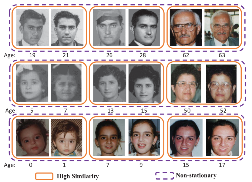
Figure 1: Facial images at different ages. The images of each row come from the same person. On the one hand, we can see the non-stationary property of aging patterns. The facial aging process is mainly reflected in the shape of the face during childhood and skin texture during adulthood. On the other hand, the facial images at adjacent ages show a very high similarity caused by the continuous aging process.

Age estimation can be cast as a regression problem by treating age labels as numerical values. However, the human face matures in different ways at different ages, e.g., bone growth in childhood and skin wrinkles in adulthood [28]. This non-stationary aging process implies that the data of age estimation is heterogeneous. Thus many nonlinear regression approaches[12, 15] are inevitably biased by the heterogeneous data distribution, and they are apt to overfit the training data [4]. Many efforts [34, 31, 15, 24] have been devoted to addressing this problem. Divide-and-conquer proves to be a good strategy to tackle the heterogeneous data [18], which divides the data space into multiple subspaces. Huang et al. use local regressors to learn homogeneous data partitions [18]. Many ranking based methods transform the regression problem into a series of binary classification subproblems [6, 4]. On the other hand, the facial aging process is also a continuous process, that is to say, human faces change gradually with age. Such a continuous process causes the appearance of faces to be very similar at adjacent ages. For example, the facial appearance will be very similar when you are 31 and 32. More examples are shown in Figure 1. This similarity relationship caused by continuity plays a dominant role at adjacent ages. The same phenomenon can be found in adjacent local regressors or adjacent binary classification subproblems, considering that we divide data by ages. However, this relationship is not exploited in existing methods.

In this paper, we propose a continuity-aware probabilistic network, called BridgeNet, to address the above challenges. The proposed BridgeNet consists of local regressors and gating networks. The local regressors partition the data space and gating networks provide continuity-aware weights. The mixture of weighted regression results gives the final accurate estimation. BridgeNet has many advantages. First, heterogeneous data are explicitly modeled by local regressors as a divide-and-conquer approach. Second, gating networks have a bridge-tree structure, which is proposed by introducing bridge connections into tree models to enforce the similarity between neighbor nodes on the same layer of bridge-tree. Therefore, the gating networks can be aware of the continuity between local regressors. Third, the gating networks of BridgeNet use a probabilistic soft decision instead of a hard decision, so that the ensemble of local regressors can give a precise and robust estimation. Fourth, we can jointly train local regressors and gating networks, and easily integrate BridgeNet with any deep neural networks into an end-to-end model. We validate the proposed BridgeNet for age estimation on three challenging datasets: MORPH Album II [29], FG-NET [26], and Chalearn LAP 2015 datasets [7], and the experimental results demonstrate that our approach outperforms the state-of-the-art methods.

2 Related Work

Age Estimation: Existing methods for age estimation can be grouped into three categories: regression based methods, classification based methods, and ranking based methods [25]. Regression based methods treat age labels as numerical values and utilize a regressor to regress the age. Guo et al. introduced many regression based methods for age estimation, such as SVR, PLS, and CCA [14, 13, 15]. Zhang et al. proposed the multi-task warped Gaussian process [45] to predict the age of face images. However, these universal regressors suffer from handling heterogeneous data. Hierarchical models [16] and group-specific regression have shown promising results by dividing data by ages. Huang et al. presented Soft-margin Mixture of Regression to learn homogeneous partitions and learned a local regressor for each partition [18]. But the continuity relationship between partitioned components is ignored in these methods. Classification based methods usually treat different ages or age groups as independent class labels [15]. DEX [31] cast age estimation as a classification problem with 101 categories. Therefore, the costs of any type of classification error are the same, which can’t exploit the relations between age labels. Recently, several researchers introduced ranking techniques to the problem of age estimation. These methods usually utilize a series of simple binary classifiers to determine the rank of the age for a given input face image. Then the final age value can be obtained by combining the results of these binary classification subproblems. Chang et al. [4] proposed an ordinal hyperplanes ranker to employ the information of relative order between ages. Niu et al. [24] addressed the ordinal regression problem with multiple output CNN. Chen et al. [6] presented Ranking-CNN and established a much tighter error bound for ranking based age estimation. However, the relations between binary subproblems are ignored in these methods, and ordinal regression is limited to scalar output [18].

Random Forests: Random forests [3] is a widely used classifier in machine learning and computer vision community. Their performance has been empirically demonstrated in many tasks such as human pose estimation [36] or image classification [2]. Meanwhile, deep CNN [21, 17] shows the superior performance of feature learning. Deep neural decision forests (dDNFs) were proposed in [20] to combine these two worlds. Each neural decision tree consists of several split nodes and leaf nodes. Each split node decides the routing direction in a probabilistic way, and each leaf node holds a class-label distribution. The dDNFs are differentiable, and the split nodes and leaf nodes are alternating learned using a two-step optimization strategy. As a classifier, dDNFs have shown the superior results on many classification tasks. There have been some efforts to migrate dDNFs to the regression problem. Shen et al. proposed DRF for age estimation by extending the distribution of leaf node to the continuous Gaussian distribution [34]. NRF [32] was designed for monocular depth estimation, which used CNN layers to build the structure of random forests. However, as will be mentioned in Sec. 3, it is not suitable to use tree architectures directly in some regression tasks, such as age estimation.

3 Proposed Approach

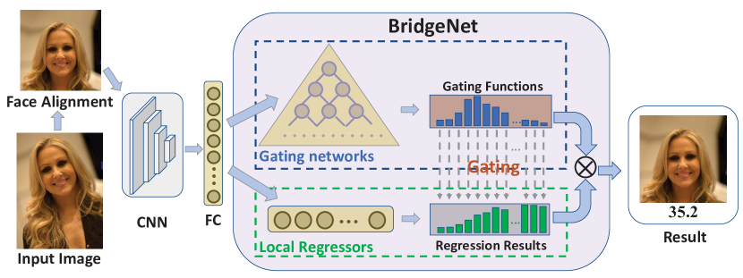
Figure 2: Flowchart of our proposed method for age estimation. For a given input image, we first apply a face alignment algorithm to get an aligned facial image. Then the aligned image is passed through a CNN for feature extraction. The extracted features are connected with two parts of BridgeNet: local regressors and gating networks separately. Gating networks generate continuity-aware gating functions to weight the regression results provided by local regressors. The final age is computed by summing the weighted regression results.

3.1 Overall Framework

The flow chart of our method is illustrated in Fig 2. For any input image $\bm{x}\in\mathcal{X}$, we first crop the human face from the image to remove the background and then align the face. The aligned face image is sent to a deep convolution neural network to extract features. Then the features are connected with two parts of BridgeNet: local regressors and gating networks separately. The final age is estimated as a weighted combination over all the local regressors.

The local regressors are utilized to handle heterogeneous data, which splits the training data into $k$ overlapping subsets. Each subset is used to learn a local regressor. We denote $\bm{y}\in\mathcal{Y}$ as the output target of input sample $\bm{x}\in\mathcal{X}$, so the regressor of the $l^{th}$ subset ($l=1,2,...,k$) can be formulated as:

$$f(\bm{y}|\bm{x},z=l)=\mathcal{N}(\bm{y}|\mu_{l}(\bm{x}),\sigma_{l}^{2}),$$ (1)

where $z$ is a latent variable that denotes the affiliation of $\{\bm{x,y}\}$ to a subset, and $\mu_{l}(\bm{x})$ denotes the regression result of the $l^{th}$ local regressor for input sample $\bm{x}$. Moreover, a Gaussian distribution $\mathcal{N}(\bm{y})$ with a mean of $\mu_{l}(\bm{x})$ and a variance of $\sigma_{l}^{2}$ is used to model the regression error.

In order to combine these regression results effectively, the gating networks with a new bridge-tree architecture are proposed, which generate a gating function for each local regressor. We denote the gating function corresponding to the $l^{th}$ local regressor as $\pi_{l}(\bm{x})$. Clearly, $\pi_{l}(\bm{x})$s are positive and $\sum_{l}\pi_{l}(\bm{x})=1$ for any $\bm{x}\in\mathcal{X}$. Then we can address age estimation by modeling the conditional probability function:

$$p(\bm{y|x})=\sum_{l}\pi_{l}(\bm{x})\mathcal{N}(\bm{y}|\mu_{l}(\bm{x}),\sigma_{l}^{2}).$$ (2)

The objective of age estimation is to find a mapping $\bm{g:x\rightarrow y}$. The output $\bm{\hat{y}}$ is estimated for an input sample $\bm{x}$ by calculating the expectation of conditional probability distribution:

$$\hat{\bm{y}} =\mathbb{E}[p(\bm{y|x})]=\mathbb{E}[\sum_{l}\pi_{l}(\bm{x})\mathcal{N}(\bm{y}|\mu_{l}(\bm{x}),\sigma_{l}^{2})]$$ (3)

$$=\sum_{l}\pi_{l}(\bm{x})\mu_{l}(\bm{x}).$$

So the sum of regression results weighted by gating functions gives the final estimated age. In the following sections, we will provide a detailed description of how local regressors and gating networks generate regression results and continuity-aware gating functions respectively.

3.2 Local Regressors

As a divide-and-conquer approach, local regressors can be used to model heterogeneous data effectively. Local regressors divide the data space into multiple subspaces, and each local regressor only performs regression on one subspace. We can regard local regressors as multiple experts. Each expert has good knowledge in a small regression region, and different experts cover different regression regions. So the ensemble of experts can give a desirable result even with heterogeneous data.

Here, we divide data by age labels, and each regressor is assigned data in an age group. The mediums of the regression regions of local regressors are evenly distributed throughout the whole regression space, and all local regressors have the same length of regression region.

To further model the continuity of age labels, we let the regression regions of local regressors are densely overlapped. The adjacent local regressors have a very high overlap in their responsible regions, which makes them have a high similarity. Therefore, for any value, there are multiple regressors responsible for regressing it, which allows us to employ ensemble learning to make the regression result more accurate.

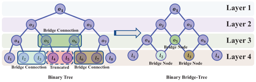
(a) Illustration how to build a four-layer binary bridge-tree. Node $o_{5}$ and $o_{6}$, node $l_{2}$ and $l_{3}$, node $l_{6}$ and $l_{7}$ in the binary tree are merged into node $o_{5}$, $l_{2}$ and $l_{3}$ in the binary bridge-tree respectively. Node $l_{4}$ and $l_{5}$ are truncated.

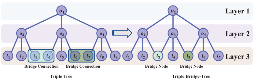
(b) Illustration how to build a three-layer triple bridge-tree. Node $l_{3}$ and $l_{4}$, node $l_{6}$ and $l_{7}$ in the triple tree are merged into node $l_{3}$ and $l_{5}$ in the triple bridge-tree respectively.

Figure 3: Illustration how to build a bridge-tree

3.3 Gating Networks

Bridge Connections: The design of local regressors follows the principle of divide-and-conquer. In our approach, gating networks are required to decide the weights of local regressors. Therefore, using gating networks with a divide-and-conquer architecture makes the gating networks and local regressors better cooperate with each other. The tree structure is a widely used hierarchical architecture with the divide-and-conquer principle. For example, the decision tree is a popular classifier in machine learning and computer vision community, which has a tree structure and a coarse-to-fine decision-making process.

On the other hand, there is a continuity relationship between local regressors due to the continuous aging process. The design of densely overlapped local regressors further strengthens this relationship. However, directly using tree structure can not well model this relationship between local regressors, considering that the leaves of the decision tree are independent class labels, while the leaves of our method are local regressors with a strong relationship. For example, the leaf node $l_{4}$ and $l_{5}$ in the left side of Figure 3(a) are adjacent leaf nodes, but their first common ancestor node is the root node, so the similarity between $l_{4}$ and $l_{5}$ caused by continuity can’t be well modeled.

We introduce bridge connections into tree models to enforce the similarity between neighbor nodes. For two adjacent nodes on the same layer, the rightmost child of the left node and the leftmost child of the right node are merged into one node. We call this operation a bridge connection because it connects two distant nodes like a bridge. The merged point, which is named bridge node here, plays a role in communicating information between the child nodes of the left node and the child nodes of the right node. By applying this operation to a tree model layer by layer, a new continuity-aware structure named bridge-tree is obtained.

Figure 3(a) shows how to get a 4-layer binary bridge-tree by applying bridge connections to a 4-layer binary tree. We can see in the binary bridge-tree that the rightmost child of node $o_{2}$ and the leftmost child of node $o_{3}$ are merged into node $o_{5}$. Bridge node $o_{5}$ is the information communication bridge between the child nodes of node $o_{2}$ and the child nodes of node $o_{3}$. The same operation is applied to node $l_{2}$ and $l_{3}$, node $l_{6}$ and $l_{7}$ in the binary tree. They are merged into node $l_{2}$ and $l_{3}$ in binary bridge-tree respectively. Node $l_{4}$ and $l_{5}$ in binary tree are truncated because that node $o_{5}$ and $o_{6}$ in the binary tree have already been merged into one node. Furthermore, the bridge connection can be applied to multiway tree to get multiway bridge-tree. Especially, Figure 3(b) gives another example of how to build a triple bridge-tree. It is worth noting that the growth rate of node number of the triple bridge-tree is very close to that of the binary tree.

Gating Functions: In this section, we will describe how to use bridge-tree structured gating networks to generate continuity-aware gating functions. Bridge-tree contains two types of nodes: decision (or split) nodes and prediction (or leaf) nodes. The decision nodes indexed by $\mathcal{O}$ are internal nodes, and the prediction nodes indexed by $\mathcal{L}$ are the terminal nodes. Each prediction node $l\in\mathcal{L}$ corresponds to a regression result $\mu_{l}(\bm{x})$ and a gating function $\pi_{l}(\bm{x})$. The regression results are given by local regressors while the gating functions are given by gating networks.

To facilitate the later parts of this paper, $\mathcal{N}$ is used to index all nodes in bridge-tree and $\mathcal{E}$ is used to index all edges in bridge-tree. We also denote $F_{n}$ and $C_{n}$ as the parent nodes set and the child nodes set of node $n\in\mathcal{N}$, respectively. When a sample $\bm{x}\in\mathcal{X}$ reaches a decision node $o$, it will be sent to the children of this node. Following [20, 34, 35], we use a probabilistic soft decision. Every edge $e\in\mathcal{E}$ is attached with a probability value. The edges connecting decision node $o$ and its child nodes form a decision probability distribution at node $o$. So that means $e_{o}^{m}(\bm{x})$s are positive for any node $m\in C_{o}$ and $\sum_{m\in C_{o}}e_{o}^{m}(\bm{x})=1$, where $e_{o}^{m}(\bm{x})$ represents the probability value which sits at the edge from node $o$ to node $m$. Once a sample ends in a leaf node $l$, the gating function for leaf node $l$ can be obtained by accumulating all the probability values of the path from the root node to the leaf node $l$. For example, there are three paths from root node $o_{1}$ to leaf node $l_{2}$ in the binary bridge-tree in Figure 3(a): $o_{1}-o_{2}-o_{4}-l_{2}$, $o_{1}-o_{2}-o_{5}-l_{2}$, and $o_{1}-o_{3}-o_{5}-l_{2}$. So the gating function for leaf node $l_{2}$ can be computed as $\pi_{l_{2}}(\bm{x})=e_{o_{1}}^{o_{2}}(\bm{x})e_{o_{2}}^{o_{4}}(\bm{x})e_{o_{4}}^{l_{2}}(\bm{x})+e_{o_{1}}^{o_{2}}(\bm{x})e_{o_{2}}^{o_{5}}(\bm{x})e_{o_{5}}^{l_{2}}(\bm{x})+e_{o_{1}}^{o_{3}}(\bm{x})e_{o_{3}}^{o_{5}}(\bm{x})e_{o_{5}}^{l_{2}}(\bm{x})$. Moreover, we give a recursive expression of gating function by extending the definition of gating function to all nodes $n\in\mathcal{N}$:

$$\pi_{n_{0}}(\bm{x})=1$$ (4)

$$\pi_{n}(\bm{x})=\sum_{m\in F_{n}}\pi_{m}(\bm{x})e_{m}^{n}(\bm{x}),$$ (5)

where $\pi_{n}(\bm{x})$ denotes the gating function for node $n$ and node $n_{0}$ is the root node of bridge-tree. We establish a one-to-one correspondence between the gate networks and the probability values on the edges of bridge-tree, that is to say, every gating network corresponds to a probability value which sits at an edge of the bridge-tree. Then the gating functions for leaf nodes can be calculated using the outputs of gating networks in the above recursive way.

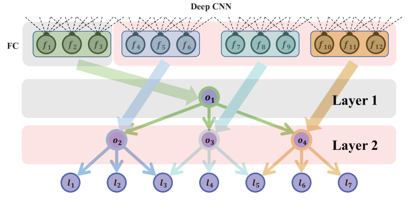
Figure 4: Illustration how to implement gating networks. An FC layer connected with deep CNN is employed. Each neuron in the fully-connected layer corresponds to an edge of bridge-tree. For example, neural $f_{1}$, $f_{2}$ and $f_{3}$ correspond to edge $o_{1}$-$o_{2}$, $o_{1}$-$o_{3}$, and $o_{1}$-$o_{4}$ respectively. For the triple bridge-tree, every three neurons are normalized using a softmax layer. Then the normalized outputs of neurons give all the probability values on the edges of bridge-tree. Finally, the gating functions for leaf nodes are calculated using Eq. 4 and Eq. 5.

3.4 Implementation Details

We employ a fully-connected layer to implement densely overlapped local regressors. The sigmoid function is utilized as the activation function. Then each local regressor maps the activation value to their regression space as the expert result. As mentioned above, we use $\mu_{l}(\bm{x})$ to denote the result of the $l^{th}$ local regressor , then the regression loss is given by:

$$L_{reg}(\bm{x,y})=\sum_{l\in\mathcal{L}}{\mathbb{I}}_{l}(\bm{x,y})(\bm{y}-\mu_{l}(\bm{x}))^{2},$$ (6)

where ${\mathbb{I}}_{l}(\bm{x,y})$ denotes if $\bm{y}$ is located in the responsible region of the $l^{th}$local regressor.

Figure 4 demonstrates the implementation of gating networks, which also employs a fully-connected layer. Each neuron in the fully-connected layer corresponds to an edge of bridge-tree. We let $B$ represents the number of branches of each decision node. Considering that $B$ edges starting from the same node form a probability distribution, we apply a softmax function to every $B$ neurons of the fully connected layer for normalization. The gating functions of leaf nodes can be calculated using these normalized outputs of neurons according to Eq. 4 and Eq. 5.

Since the ground truth for supervising gating functions is not available, we build approximated gating targets for an input sample $(\bm{x,y})$ as follow:

$$\hat{\pi}_{l}(\bm{x})=\frac{1}{R}{\mathbb{I}}_{l}(\bm{x,y}),$$ (7)

where $R=\sum_{l}{\mathbb{I}}(\bm{x,y})$ is used for normalization. Although the labels are not accurate, our gating networks can be aware of the continuity between local regressors, so a satisfying result can be achieved even with weakly supervised signals.

The KL divergence is utilized as the loss term to train the gating networks of BridgeNet:

$$L_{gate}(\bm{x,y})=-\sum_{l\in\mathcal{L}}\hat{\pi}_{l}(\bm{x})\log(\pi_{l}(\bm{x})).$$ (8)

In the end, we jointly learn local regressors and gating networks by defining the total loss as follow:

$$L_{total}(\bm{x,y})=L_{reg}(\bm{x,y})+\lambda L_{gate}(\bm{x,y}),$$ (9)

where $\lambda$ is used to balance the importance between the regression task and gating task.

We observe that the proposed BridgeNet can be easily implemented by using typically available fully-connected, softmax and sigmoid layers in the existing deep learning frameworks such as TensorFlow [1], PyTorch [27], etc. Furthermore, our fully differentiable BridgeNet can be embedded within any deep convolutional neural networks, which enables us to conduct end-to-end training and obtain a better feature representation.

4 Experiments

In this section, we first introduce the datasets and present some details about our experiment settings. Then we demonstrate the experimental results to show the effectiveness of the proposed BridgeNet.

4.1 Datasets

MORPH II is the largest publicly available longitudinal face dataset and the most popular dataset for age estimation. This dataset includes more than 55,000 images from about 13,000 subjects and age ranges from 16 to 77 years.

In this paper, two widely used protocols are employed for evaluation on MORPH II. The first setting uses a subset of MORPH II as described in [4, 5, 41]. This setting selects 5,492 images of people of Caucasian descent to avoid the cross-race influence. Then these 5,492 images are randomly divided into two non-overlapped parts: 80% of data for training and 20% of data for testing. The second setting used in [43, 13] randomly splits the whole MORPH II dataset into three non-overlapped subsets $S1,S2,S3$ following the rules detailed in [43]. The training and testing are repeated twice in this setting: 1) training on $S1$, testing on $S2+S3$ and 2) training on $S2$, testing on $S1+S3$. We will report the performance of these two experiments and their average.

FG-NET consists of 1002 color or greyscale face images of 82 individuals with ages ranging from 0 to 69 years old subjects. For evaluation, we adopt the setup of [12, 31], which uses leave-one person-out (LOPO) cross-validation. The average performance over 82 splits is reported.

Chalearn LAP 2015 is the first dataset on apparent age estimation. For any image, at least 10 independent users are required to give their opinions and then the average age is used as the annotation. Additionally, the standard deviation of opinions for a given image is also provided. This dataset contains 4699 images, where 2476 images for training, 1136 images for validation, and 1087 images for testing. The age range is from 0 to 100 years old.

IMDB-WIKI contains more than half a million labeled images of celebrities, which are crawled from IMDb and Wikipedia. This datatset contains too much noise, so it is not suitable for evaluation. However, it is still a good choice to use this dataset for pretraining after data cleaning. We select about 200 thousand images according to the setting in [31] to pre-train our network.

Table 1: The comparisons between the proposed method and other state-of-the-art methods on MORPH II dataset (setting I) and FG-NET dataset.

Method	MORPH II	FG-NET	Year
Human [16]	6.30	4.70	-
AGES [8]	8.83	6.77	2007
IIS-LDL [10]	-	5.77	2010
CPNN [11]	-	4.76	2013
MTWGP [45]	6.28	4.83	2010
OHRank [4]	6.07	4.48	2011
CA-SVR [5]	5.88	4.67	2013
DRFs [34]	2.91	3.85	2018
DEX [31]	2.68	3.09	2016
Pan et al. [25]	-	2.68	2018
BridgeNet	2.38	2.56	-

Table 2: The results on MORPH II dataset (setting II). The performance of two different settings and their average are reported. Our method achieves the state-of-the-art performance.

Method	Train	Test	MAE	Avg
KPLS [13]	S1	S2+S3	4.21	4.18
	S2	S1+S3	4.15
BIF+KCCA [14]	S1	S2+S3	4.00	3.98
	S2	S1+S3	3.95
CPLF [43]	S1	S2+S3	3.72	3.63
	S2	S1+S3	3.54
Tan et al. [40]	S1	S2+S3	3.14	3.03
	S2	S1+S3	2.92
DRFs [34]	S1	S2+S3	-	2.98
	S2	S1+S3	-
BridgeNet	S1	S2+S3	2.74	2.63
	S2	S1+S3	2.51

Table 3: Comparisons with the state-of-the-art methods on the Chalearn LAP 2015 dataset

Rank	Team	Validation Set		Test Set		Pretrain	Netwrok	# of
		MAE	$\epsilon$-error	MAE	$\epsilon$-error	Set		Networks
-	BridgeNet	2.98	0.26	2.87	0.255140	IMDB-WIKI	VGG-16	1
-	Tan et al. [39]	3.21	0.28	2.94	0.263547	IMDB-WIKI	VGG-16	8
1	CVL_ETHZ [31]	3.25	0.28	-	0.264975	IMDB-WIKI	VGG-16	20
2	ICT-VIPL [23]	3.33	0.29	-	0.270685	MORPH, CACD, et al.	GoogleNet	8
3	WVU_CVL [46]	-	0.31	-	0.294835	MORPH, CACD, et al.	GoogleNet	5
4	SEU_NJU [42]	-	0.34	-	0.305763	FG-NET,MORPH,et al.	GoogleNet	6
	Human	-	-	-	0.34	-	-	-

4.2 Experimental Settings

Face alignment is a common preprocessing step for age estimation. First, all images are sent to MTCNN [44] for face detection. Then we align all the face images by similarity transformation based on the detected five facial landmarks. After that, all images are resized into $256\times 256$.

Data augmentation is an effective way to avoid overfitting and improve the generalization of deep networks, especially when the training data is insufficient. Here, we augment training images with horizontal flipping and random cropping.

VGG-16 [37] is employed as the basic backbone network of the proposed method. We first initialize the VGG-16 network with the weights from training on ImageNet 2012 [33] dataset. Then the network is pre-trained on IMDB-WIKI dataset. To optimize the proposed network, we use the mini-batch stochastic gradient descent (SGD) with batch size 64 and apply the Adam optimizer [19]. The initial learning rate is set to 0.0001 for experiments on MORPH II dataset. The training images on FG-NET and Chalearn LAP 2015 datasets are extremely insufficient, so we set the initial learning rate of CNN part to 0.00001 for the experiments on these datasets to avoid overfitting. The initial learning rate of the BridgeNet part is still 0.0001 on these datasets to accelerate convergence. We train our network for 60 epochs and set $\lambda$ to 0.001 to balance the gating loss and regression loss. The length of regression region for local regressors is set to 25. We choose a triple bridge-tree with a depth of 5 as the architecture of our BridgeNet, which is a trade-off of efficiency and complexity. Our algorithm is implemented within the PyTorch [27] framework. A GeForce GTX 1080Ti GPU is used for neural network acceleration.

4.3 Evaluation Metrics

The mean absolute error (MAE) and cumulative score (CS) are used as evaluation metrics on MORPH II and FG-NET datasets. MAE is calculated using the mean absolute errors between the estimated result and ground truth: $MAE=\frac{1}{K}\sum_{i=1}^{K}|\bm{y_{i}^{\prime}}-\bm{y_{i}}|$, where $\bm{y_{i}^{\prime}}$ denotes the predicted age value for the $i^{th}$ image, and $K$ is the number of testing samples. Obviously, a lower MAE result means better performance. $CS(\theta)$ is computed as follows: $CS(\theta)=\frac{K_{\theta}}{K}$, where $K_{\theta}$ represents the number of test images whose absolute error between the estimated result and the ground truth is not greater than $\theta$ years. Naturally, the higher the $CS(\theta)$, the better performance it gets. The $\epsilon$-error was proposed by the Chalearn LAP challenge as a quantitative measure, which is defined as: $\epsilon=1-\frac{1}{K}\sum_{i=1}^{K}e^{-\frac{(\bm{y_{i}^{\prime}-y_{i}})^{2}}{2\sigma_{i}^{2}}}$, where $\sigma_{i}$ is the standard deviation of the $i^{th}$ image. Clearly, a lower $\epsilon$-error means better performance.

4.4 Results and Analysis

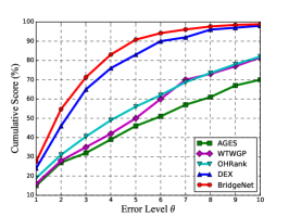
(a) MORPH II (setting I)

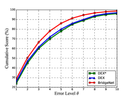
(b) MORPH II (setting II)

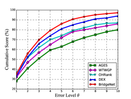
(c) FG-NET

Figure 5: (a) CS curves compared with other methods on MORPH II dataset with setting I. (b)CS curves compared with other methods on MORPH II dataset with setting II. * means that the IMDB-WIKI dataset was not used to pre-train the model. (c) CS curves compared with other methods on FG-NET.

Table 4: The comparisons of different architectures on MORPH II dataset (setting I)

Architecture	Softmax				Tree(binary)				Bridge-Tree(triple)
Depth	-				4	5	6	7	3	4	5	6
Num. of leaf nodes	16	32	64	128	16	32	64	128	15	31	63	127
Num. of decision nodes	-				15	31	63	127	11	26	57	120
MAE	2.68	2.59	2.54	2.53	2.66	2.54	2.51	2.49	2.51	2.43	2.38	2.38

Table 5: The results of binary bridge-tree structure on MORPH II dataset (setting I)

Num. of leaf nodes	16	32	64	128
MAE	2.43	2.39	2.36	2.35

Comparisons with the State-of-the-art: We first compare the proposed BridgeNet with other state-of-the-art methods on MORPH II dataset with different settings and FG-NET dataset. Table 1 and Table 2 show the results on MORPH II and FG-NET using MAE metric. The results demonstrate that our method outperforms the state-of-the-art methods with a clear margin on both datasets. Our method achieves the lowest MAE of 2.38, 2.63, and 2.56 on MORPH II with setting I, MORPH II with setting II, and FG-NET respectively. The classification based methods, such as DEX [31], Tan et al. [40], are not optimal because they treat different ages as independent class labels. On the other hand, the ranking based methods, such as OHRank [4], can’t capture the continuity relationship among components, resulting in unsatisfactory performance. DRFs [34] uses a tree structure to weight several Gaussian distributions and Pan et al. propose a mean-variance loss for age estimation. Both of them can’t effectively model the continuous property of the aging process. The CS comparisons with the state-of-the-art methods on MORPH II and FG-NET are shown in Figure 5. The experimental results show that our approach consistently outperforms other methods.

In addition to these two datasets, we present results of our method on Chalearn LAP 2015 dataset. Following [31, 30, 39], a few tricks are used on this competition dataset. To get the performance on the test set, we finetune our network on both training and validation sets after finetuning on IMDB-WIKI dataset. In the test phase, for any given image, we crop it into four corners and a central crop, then the five crops plus the flipped version of these are sent to our network, and these ten predictions are averaged. It is important to note that we only use these tricks on Chalearn LAP 2015 dataset. To make a more comprehensive comparison, we also show the performance on the validation set, which only uses the training set to finetune. The experimental results are shown in Table 3. The bottom half of the table shows the results of the participating teams, and the top half shows the results of our method and another state-of-the-art method. We can see that our method achieves better performance than other methods. Our method achieves an MAE of 2.98 and a $\epsilon$-error of 0.26 on the validation set, which reduces the state-of-the-art performance by 0.23 years for MAE and 0.02 for $\epsilon$-error. For the test set, we also achieve a lower MAE and $\epsilon$-error. All of the above results of our method are obtained by using a single network, while others methods use an ensemble of multiple networks, which further illustrates the superiority of our method.

Ablation Study and Parameters Discussion: To validate the effectiveness of the proposed BridgeNet, we compare it with two baseline architectures: one uses a tree structure to construct gating functions, and the other uses a softmax layer to construct gating functions. To be fair, we use triple bridge-tree structure, whose node growth rate is close to that of the binary tree. The experiments are conducted on MORPH II dataset (setting I) and Table 4 shows the results.

Several conclusions are drawn from Table 4. First, in any of the above architectures, a lower MAE can be obtained by using more leaf nodes, which is reasonable because more leaf nodes mean more local regressors and more local regressors mean more expert intelligence. Furthermore, when the number of leaf nodes is large enough, the performance tends to be saturated. This is because too many leaf nodes make some adjacent local regressors correspond to the same training data, so it can not increase the actual number of experts. Second, we observe that the tree-based method slightly outperforms the softmax based method when the number of leaf nodes is the same. The tree-based method has a coarse-to-fine, top-to-down decision-making process as a hierarchical architecture, so it can give better performance than softmax based method. However, it doesn’t explicitly model the continuity relationship between local regressors, so the performance gain is tiny. Third, bridge-tree based method (BridgeNet) significantly outperforms the tree-based method at a similar number of leaf nodes even with a shallower depth and fewer decision nodes. The five layers triple bridge-tree achieves an MAE of 2.38, which reduces the MAE by 0.13 years compared with the six layers binary tree. This shows the benefit of introducing bridge connections and explicitly modeling the continuity relation.

To further demonstrate the superiority of bridge-tree, we show the results using binary bridge-tree architecture on MORPH II dataset (setting I) in Table 5. We can see that binary bridge-tree further improves the accuracy. This is because, with the same number of leaf nodes, binary bridge-tree has more bridge nodes, which makes it better capture the continuity relationship between local regressors.

5 Conclusions

In this paper, we have presented BridgeNet, a continuity-aware probabilistic network for age estimation. BridgeNet explicitly models the continuity relationship between different components constructed by local regressors using a probabilistic network with a bridge-tree architecture. Experiments on three datasets demonstrate that our method is more accurate than other state-of-the-art methods. Although our method is designed for age estimation, it can also be used for other regression-based computer vision tasks. In the future work, we plan to investigate the effectiveness of BridgeNet in crowd counting, pose estimation and other regression-based tasks.

References

- [1] M. Abadi, A. Agarwal, P. Barham, E. Brevdo, Z. Chen, C. Citro, G. S. Corrado, A. Davis, J. Dean, and M. Devin. Tensorflow: Large-scale machine learning on heterogeneous distributed systems. 2016.
- [2] A. Bosch, A. Zisserman, and X. Munoz. Image classification using random forests and ferns. In ICCV, pages 1–8, 2007.
- [3] L. Breiman. Random forests. Machine Learning, 45(1):5–32, 2001.
- [4] K. Y. Chang, C. S. Chen, and Y. P. Hung. Ordinal hyperplanes ranker with cost sensitivities for age estimation. In CVPR, pages 585–592, 2011.
- [5] K. Chen, S. Gong, T. Xiang, and C. L. Chen. Cumulative attribute space for age and crowd density estimation. In CVPR, pages 2467–2474, 2013.
- [6] S. Chen, C. Zhang, M. Dong, J. Le, and M. Rao. Using ranking-cnn for age estimation. In CVPR, pages 742–751, 2017.
- [7] S. Escalera, J. Fabian, P. Pardo, X. Baro, J. Gonzalez, H. J. Escalante, D. Misevic, U. Steiner, and I. Guyon. Chalearn looking at people 2015: Apparent age and cultural event recognition datasets and results. In ICCVW, pages 243–251, 2015.
- [8] Geng, Xin, Zhou, ZhiHua, SmithMiles, and Kate. Automatic age estimation based on facial aging patterns. TPAMI, 29(12):2234–2240, 2007.
- [9] Geng, Xin, Zhou, ZhiHua, Zhang, Yu, Li, Gang, and Dai. Learning from facial aging patterns for automatic age estimation. ACM MM, pages 307–316, 2006.
- [10] X. Geng, C. Yin, and Z. H. Zhou. Facial age estimation by learning from label distributions. In AAAI, pages 451–456, 2010.
- [11] X. Geng, C. Yin, and Z. H. Zhou. Facial age estimation by learning from label distributions. TPAMI, 35(10):2401–2412, 2013.
- [12] G. Guo, Y. Fu, C. R. Dyer, and T. S. Huang. Image-based human age estimation by manifold learning and locally adjusted robust regression. TIP, 17(7):1178–1188, 2008.
- [13] G. Guo and G. Mu. Simultaneous dimensionality reduction and human age estimation via kernel partial least squares regression. In CVPR, pages 657–664, 2011.
- [14] G. Guo and G. Mu. Joint estimation of age, gender and ethnicity: Cca vs. pls. In FG, pages 1–6, 2013.
- [15] G. Guo, G. Mu, Y. Fu, and T. S. Huang. Human age estimation using bio-inspired features. In CVPR, pages 112–119, June 2009.
- [16] H. Han, C. Otto, X. Liu, and A. K. Jain. Demographic estimation from face images: Human vs. machine performance. TPAMI, 37(6):1148–1161, 2015.
- [17] K. He, X. Zhang, S. Ren, and J. Sun. Deep residual learning for image recognition. In CVPR, pages 770–778, 2016.
- [18] D. Huang, L. Han, and F. D. L. Torre. Soft-margin mixture of regressions. In CVPR, pages 4058–4066, 2017.
- [19] D. P. Kingma and J. Ba. Adam: A method for stochastic optimization. Computer Science, 2014.
- [20] P. Kontschieder, M. Fiterau, A. Criminisi, and S. Rota Bulo. Deep neural decision forests. In ICCV, pages 1467–1475, 2015.
- [21] A. Krizhevsky, I. Sutskever, and G. E. Hinton. Imagenet classification with deep convolutional neural networks. In NIPS, pages 1097–1105, 2012.
- [22] A. Lanitis, C. Draganova, and C. Christodoulou. Comparing different classifiers for automatic age estimation. TSMC, Part B (Cybernetics), 34(1):621–628, Feb 2004.
- [23] X. Liu, S. Li, M. Kan, J. Zhang, S. Wu, W. Liu, H. Han, S. Shan, and X. Chen. Agenet: Deeply learned regressor and classifier for robust apparent age estimation. In ICCVW, pages 258–266, 2015.
- [24] Z. Niu, M. Zhou, L. Wang, X. Gao, and G. Hua. Ordinal regression with multiple output cnn for age estimation. In CVPR, pages 4920–4928, 2016.
- [25] H. Pan, H. Han, S. Shan, and X. Chen. Mean-variance loss for deep age estimation from a face. In CVPR, June 2018.
- [26] G. Panis, A. Lanitis, N. Tsapatsoulis, and T. F. Cootes. Overview of research on facial ageing using the fg-net ageing database. Iet Biometrics, 5(2):37–46, 2016.
- [27] A. Paszke, S. Gross, S. Chintala, G. Chanan, E. Yang, Z. DeVito, Z. Lin, A. Desmaison, L. Antiga, and A. Lerer. Automatic differentiation in pytorch. 2017.
- [28] N. Ramanathan, R. Chellappa, and S. Biswas. Age progression in human faces : A survey. JVLC, 15, 2009.
- [29] K. Ricanek and T. Tesafaye. Morph: a longitudinal image database of normal adult age-progression. In FG, pages 341–345, 2006.
- [30] R. Rothe, R. Timofte, and L. V. Gool. Dex: Deep expectation of apparent age from a single image. In ICCVW, December 2015.
- [31] R. Rothe, R. Timofte, and L. V. Gool. Deep expectation of real and apparent age from a single image without facial landmarks. IJCV, pages 1–14, 2016.
- [32] A. Roy and S. Todorovic. Monocular depth estimation using neural regression forest. In CVPR, pages 5506–5514, 2016.
- [33] O. Russakovsky, J. Deng, H. Su, J. Krause, S. Satheesh, S. Ma, Z. Huang, A. Karpathy, A. Khosla, and M. Bernstein. Imagenet large scale visual recognition challenge. IJCV, 115(3):211–252, 2015.
- [34] W. Shen, Y. Guo, Y. Wang, K. Zhao, B. Wang, and A. L. Yuille. Deep regression forests for age estimation. In CVPR, June 2018.
- [35] W. Shen, K. ZHAO, Y. Guo, and A. L. Yuille. Label distribution learning forests. In I. Guyon, U. V. Luxburg, S. Bengio, H. Wallach, R. Fergus, S. Vishwanathan, and R. Garnett, editors, NIPS, pages 834–843. 2017.
- [36] J. Shotton, R. Girshick, A. Fitzgibbon, T. Sharp, M. Cook, R. Moore, R. Moore, P. Kohli, A. Criminisi, and A. Kipman. Efficient human pose estimation from single depth images. TPAMI, 35(12):2821–2840, 2013.
- [37] K. Simonyan and A. Zisserman. Very deep convolutional networks for large-scale image recognition. In ICLR, 2015.
- [38] Z. Song, B. Ni, D. Guo, T. Sim, and S. Yan. Learning universal multi-view age estimator using video context. In ICCV, pages 241–248, Nov 2011.
- [39] Z. Tan, J. Wan, Z. Lei, R. Zhi, G. Guo, and S. Z. Li. Efficient group-n encoding and decoding for facial age estimation. TPAMI, PP(99):1–1, 2017.
- [40] Z. Tan, S. Zhou, J. Wan, Z. Lei, and S. Z. Li. Age estimation based on a single network with soft softmax of aging modeling. In ACCV, pages 203–216, 2017.
- [41] X. Wang, R. Guo, and C. Kambhamettu. Deeply-learned feature for age estimation. In WACV, pages 534–541, 2015.
- [42] X. Yang, B. B. Gao, C. Xing, and Z. W. Huo. Deep label distribution learning for apparent age estimation. In ICCVW, pages 344–350, 2015.
- [43] D. Yi, Z. Lei, and S. Z. Li. Age estimation by multi-scale convolutional network. In ACCV, pages 144–158, 2014.
- [44] K. Zhang, Z. Zhang, Z. Li, and Y. Qiao. Joint face detection and alignment using multitask cascaded convolutional networks. IEEE SPL, 23(10):1499–1503, 2016.
- [45] Y. Zhang and D. Y. Yeung. Multi-task warped gaussian process for personalized age estimation. In CVPR, pages 2622–2629, 2010.
- [46] Y. Zhu, Y. Li, G. Mu, and G. Guo. A study on apparent age estimation. In ICCVW, pages 267–273, 2015.