Geometry of the Hough transforms with applications to synthetic data

Abstract

In the framework of the Hough transform technique to detect curves in images, we provide a bound for the number of Hough transforms to be considered for a successful optimization of the accumulator function in the recognition algorithm. Such a bound is consequence of geometrical arguments. We also show the robustness of the results when applied to synthetic datasets strongly perturbed by noise. An algebraic approach, discussed in the appendix, leads to a better bound of theoretical interest in the exact case.

Introduction

The Hough transform is a standard technique for feature extraction used in image analysis and digital image processing. Such a technique was first used to detect straight lines in images [9]. It is based on the point-line duality as follows: points on a straight line, defined by an equation in the image plane $\langle x,y\rangle$ with the usual natural parametrization, correspond to lines in the parameter space $\langle A,B\rangle$ that intersect in a single point. This point uniquely identifies the coefficients in the equation of the original straight line (analogous procedures to detect circles and ellipses in images have been introduced in [7]). From a computational point of view, this result gives us a procedure to recognize straight lines in $2$-dimensional images in which discontinuity regions in the image are highlighted through an edge detection algorithm; the parameter space is discretized in cells and an accumulator function is defined on it, whose maximum provides us with the parameters’ values that identify the line.

Thanks to algebraic geometrical arguments, the Hough transform definition has been extended to include special classes of curves [2, 12]. In [2], a characterization of families of irreducible algebraic plane curves of the same degree for which is defined a Hough-type correspondence is provided. In fact, given a family $\mathcal{F}$ of algebraic curves, a general point $p$ in the image plane corresponds to an algebraic locus, $\Gamma_{p}(\mathcal{F})$, in the parameter space. The families $\mathcal{F}$ such that, as $p$ varies on a given curve $\mathcal{C}$ from $\mathcal{F}$, satisfy the regularity condition that the hypersurfaces $\Gamma_{p}(\mathcal{F})$ meet in one and only one point (which in turn defines the curve $\mathcal{C}$), are called Hough regular. This paper is a sequel of [2]. Indeed, in [2] the Hough transform technique was performed for the automated recognition of cubic and quartic curves, and the accuracy of the detection was tested against synthetic data. Here, the aim is to reduce the amount of the dataset to be taken into account. Furthermore, the power of this procedure is then tested on $2$-dimensional astronomical and medical real images in [12].

Let ${\mathcal{F}}=\{{\mathcal{C}}_{\bm{\lambda}}\}$ be a Hough regular family of algebraic plane curves ${\mathcal{C}}_{\bm{\lambda}}$. Let’s highlight here the steps of the standard recognition algorithm, of a given profile of interest ${\mathcal{P}}$ in a real image, on which the Hough transform technique for such families of plane curves is founded. We refer to [2, Section 6], [12, Section 4], and also [14, Section 5] for complete details.

A pre-processing step of the algorithm consists of the application of a standard edge detection technique on the image (see [6] for a detailed description of this operator). This step reduces the number of points of interest highlighting the profile ${\mathcal{P}}$ of which one has to compute the Hough transform. Then a discretization of the parameter space is required, which possibly exploits bounds on the parameter values computed by using either the Cartesian or the parametric form of the curve in the image space. A last step constructs the accumulator function after a discretization of the parameter space. The value of the accumulator in a cell of the discretized space corresponds to the number of times the Hough transforms of selected points of interest reach that cell. As a final outcome of the algorithm, the parameter values characterizing the curve best approximating the profile ${\mathcal{P}}$ in the image space correspond to the parameter values identifying the cell where the accumulator function reaches its maximum.

Thus, in practice, the computational burden associated to the accumulator function computation and optimization leads to the need of reducing as most as possible the number of points of interest to be considered. By using classical geometrical arguments we provide in Proposition 2.4, and in an exact context, a bound which quite significantly decreases the number of Hough transforms $\Gamma_{p_{j}}({\mathcal{F}})$ of points $p_{j}\in{\mathcal{C}}_{\bm{\lambda}}$ making true the regularity condition $\cap_{p_{j}}\Gamma_{p_{j}}({\mathcal{F}})=\{\bm{\lambda}\}$. This suggests to significantly bound the number of Hough transforms to be considered to recognize curves in images. Indeed, such a bound applies quite efficiently in concrete examples, and it turns out to be quite robust both in presence of noisy background and against random perturbation of points’ locations, as shown in Section 4. This significantly enhances the results of [2, Section 6], with special regard to robustness in presence of noisy background.

A better understanding of the behavior of the equations defining the Hough transforms in the parameter space leads to a refinement of Proposition 2.4. This algebraic approach provides a much better bound, called $\nu_{\rm best}$ (see Proposition A.4, Appendix A), which appears of purely theoretical interest since such a bound can be even too strong for practical purposes. Indeed, let ${\mathcal{C}}_{\bm{\lambda}}$ be a curve from a family ${\mathcal{F}}$ potentially approximating a profile ${\mathcal{P}}$. Since $\nu_{\rm best}$ can be very small (for instance, $\nu_{\rm best}=2$ in the examples provided in Appendix A), random perturbations of $\nu_{\rm best}$ point’s locations on ${\mathcal{C}}_{\bm{\lambda}}$ may produce a dataset of points not properly highlighting the profile ${\mathcal{P}}$.

The paper is organized as follows. In Section 1 we recall some background material. Section 2 is devoted to the proof of the bound mentioned above. We then provide several examples in Section 3. In Section 4, applications to synthetic data for four families of curves (the same considered in [2]) show the efficiency and the robustness of the result. Finally, our conclusions are offered in Section 5.

1 Preliminaries

Most of the results in this section hold over an infinite integral ring $K$. However, unless otherwise specified, we restrict to the case of interest in the applications, assuming either $K={\mathbb{R}}$ or $K={\mathbb{C}}$ the fields of real or complex numbers.

For every $t$-tuples of independent parameters ${\bm{\lambda}}:=(\lambda_{1},\ldots,\lambda_{t})\in K^{t}$, let

$$f_{{\bm{\lambda}}}({{\bm{x}}})=\sum_{i_{1},\ldots,i_{n}}x_{1}^{i_{1}}\ldots x_{n}^{i_{n}}g_{i_{1}\ldots i_{n}}({\bm{\lambda}}),\;\;\;\;0\leq i_{1}+\cdots+i_{n}\leq d,$$ (1)

be a family ${\mathcal{P}}$ of non-constant irreducible polynomials in the indeterminates ${{\bm{x}}}:=(x_{1},\ldots,x_{n})$, of a given degree $d$ (not depending on ${\bm{\lambda}}$), whose coefficients $g_{i_{1}\ldots i_{n}}({\bm{\lambda}})$ are the evaluation in ${\bm{\lambda}}$ of polynomials $g_{i_{1}\ldots i_{n}}({\bm{\Lambda}})\in K[{\bm{\Lambda}}]$ in a new series of indeterminates ${\bm{\Lambda}}=(\Lambda_{1},\ldots,\Lambda_{t})$. Let ${\mathcal{H}}_{\bm{\lambda}}=\{{\bm{x}}\in{\mathbb{A}}_{{\bm{x}}}^{n}(K)\>|\>f_{\bm{\lambda}}({\bm{x}})=0\}$, and let assume that ${\mathcal{H}}_{\bm{\lambda}}$ is a hypersurface for each parameter ${\bm{\lambda}}$ belonging to a Euclidean open subset ${\mathcal{U}}\subseteq K^{t}$ (of course, this is always the case if the base field is $K={\mathbb{C}}$). Clearly, if $K={\mathbb{C}}$, such hypersurfaces are irreducible, that is, they consist of a single component, since the polynomials of the family ${\mathcal{P}}$ are assumed to be irreducible in $K[{{\bm{x}}}]$. If $K={\mathbb{R}}$, the case of interest in the applications, we assume that ${\mathcal{H}}_{\bm{\lambda}}$ is a real hypersurface, that is, a hypersurface over ${\mathbb{C}}$ with a real $(n-1)$-dimensional component in the affine space ${\mathbb{A}}_{{\bm{x}}}^{n}({\mathbb{R}})$ (see [4, Theorem 4.5.1] for explicit conditions equivalent to our assumption).

Since the polynomials $f_{\bm{\lambda}}({\bm{x}})$ are irreducible over $K$, the zero loci ${\mathcal{H}}_{\bm{\lambda}}$ are irreducible up to components of dimension $\leq n-2$, that is, they consist of a single $(n-1)$-dimensional component (see [14, Remark 1.5] for related comments in the cases $n=2$ and $n=3$, respectively).

So, we assume $\mathcal{F}$ to be a family of irreducible hypersurfaces $($with possibly a finite set of lower dimensional components$)$ which share the degree.

Definition 1.1.

Let $\mathcal{F}$ be a family of hypersurfaces ${\mathcal{H}}_{\bm{\lambda}}$ as above, and let $p=(x_{1}(p),\ldots,x_{n}(p))$ be a point in the image space ${\mathbb{A}}_{{\bm{x}}}^{n}(K)$. Let ${\Gamma}_{p}(\mathcal{F})$ be the locus defined in the affine $t$-dimensional parameter space ${\mathbb{A}}_{\bm{\Lambda}}^{t}(K)$ by the polynomial equation

$$f_{p}(\bm{\Lambda})=\sum_{i_{1},\ldots,i_{n}}x_{1}(p)^{i_{1}}\ldots x_{n}(p)^{i_{n}}g_{i_{1}\ldots i_{n}}({\bm{\Lambda}})=0,\;\;\;\;\;\;0\leq i_{1}+\cdots+i_{n}\leq d.$$

We say that ${\Gamma}_{p}(\mathcal{F})$ is the Hough transform of the point $p$ with respect to the family $\mathcal{F}$. If no confusion will arise, we simply say that ${\Gamma}_{p}(\mathcal{F})$ is the Hough transform of $p$.

See also Appendix A for more details on degree and dimension of the Hough transform.

Summarizing, the polynomials family defined by (1) leads to a polynomial $F({{\bm{x}}};{\bm{\Lambda}})\in K[{{\bm{x}}};{\bm{\Lambda}}]$ whose evaluations at points ${\bm{\lambda}}\in{\mathcal{U}}$ and $p=(x_{1}(p),\ldots,x_{n}(p))\in{\mathbb{A}}_{{\bm{x}}}^{n}(K)$ give back the equations of ${\mathcal{H}}_{\bm{\lambda}}$ and ${\Gamma}_{p}(\mathcal{F})$, respectively. That is,

$${\mathcal{H}}_{\bm{\lambda}}:F({{\bm{x}}};{\bm{\lambda}})=f_{\bm{\lambda}}({{\bm{x}}})=0\;\;\;\;{\rm and}\;\;\;\;{\Gamma}_{p}(\mathcal{F}):F(p;{\bm{\Lambda}})=f_{p}(\bm{\Lambda})=0.$$

And, clearly, the following “duality condition” holds true:

$$p\in{\mathcal{H}}_{\bm{\lambda}}\Longleftrightarrow f_{\bm{\lambda}}(x_{1}(p),\ldots,x_{n}(p))=F(x_{1}(p),\ldots,x_{n}(p);\lambda_{1},\ldots,\lambda_{t})=0\Longleftrightarrow\bm{\lambda}\in\Gamma_{p}(\mathcal{F}).$$ (2)

One may note that one classically refers to the variety ${\bf I}\subset{\mathbb{A}}_{{\bm{x}}}^{n}(K)\times\mathcal{U}$ defined by the polynomial $F({{\bm{x}}};{\bm{\Lambda}})$ as incidence correspondence, or incidence variety. It consists of the pairs of points $(p,\bm{\lambda})$ such that $p\in{\mathcal{H}}_{\bm{\lambda}}$ or, equivalently, $\bm{\lambda}\in\Gamma_{p}(\mathcal{F})$. In particular, denoting by ${\pi_{1}}_{|\bf I}:{\bf I}\to{\mathbb{A}}_{{\bm{x}}}^{n}(K)$, ${\pi_{2}}_{|\bf I}:{\bf I}\to\mathcal{U}$ the restrictions to ${\bf I}$ of the product projections $\pi_{1}$, $\pi_{2}$ on the two factors, one has ${\pi_{1}}_{|{\bf I}}(\pi_{2}^{-1}(\bm{\lambda}))={\mathcal{H}}_{\bm{\lambda}}$ and, similarly, ${\pi_{2}}_{|{\bf I}}(\pi_{1}^{-1}(p))=\Gamma_{p}(\mathcal{F})$ (see also [3]).

The following general facts hold true (see [2, Theorem 2.2, Lemma 2.3], [3, Section 3]).

1. The Hough transforms ${\Gamma}_{p}(\mathcal{F})$, when the point $p$ varies on ${\mathcal{H}}_{\bm{\lambda}}$, all pass through the point ${\bm{\lambda}}$.

2. Assume that the Hough transforms ${\Gamma}_{p}(\mathcal{F})$, when $p$ varies on ${\mathcal{H}}_{\bm{\lambda}}$, have a point in common other than ${\bm{\lambda}}$, say ${\bm{\lambda}^{\prime}}$. Thus the two hypersurfaces ${\mathcal{H}}_{\bm{\lambda}}$, ${\mathcal{H}}_{\bm{\lambda}^{\prime}}$ coincide.

3. (Regularity property) The following conditions are equivalent:

   1. For any hypersurfaces ${\mathcal{H}}_{\bm{\lambda}}$, ${\mathcal{H}}_{\bm{\lambda}^{\prime}}$ in $\mathcal{F}$, the equality ${\mathcal{H}}_{\bm{\lambda}}={\mathcal{H}}_{\bm{\lambda}^{\prime}}$ implies ${\bm{\lambda}}={\bm{\lambda}^{\prime}}$.

   2. For each hypersurface ${\mathcal{H}}_{\bm{\lambda}}$ in $\mathcal{F}$, one has $\bigcap_{p\in{\mathcal{H}}_{\bm{\lambda}}}{\Gamma}_{p}(\mathcal{F})=\{\bm{\lambda}\}$.

A family $\mathcal{F}$ which meets one of the above equivalent conditions (a), (b) is said to be Hough regular.

From now on throughout the paper, we consider the case $n=2$. Let ${\bm{x}}=(x,y)$, and let $\mathcal{F}=\{{\mathcal{C}}_{\bm{\lambda}}\}$ be a family of irreducible real curves in the image plane ${\mathbb{A}}_{(x,y)}^{2}({\mathbb{R}})$, of equation

$$f_{\bm{\lambda}}(x,y)=\sum_{i,j=0}^{d}x^{i}y^{j}g_{ij}({\bm{\lambda}}),\;\;\;\;0\leq i+j\leq d,$$ (3)

and satisfying the assumptions and the properties mentioned above (in particular, the ${\mathcal{C}}_{\bm{\lambda}}$’s are affine plane curves over ${\mathbb{C}}$ with infinitely many points in the affine plane over ${\mathbb{R}}$, see also [16, Chapter 7]).

Given a profile of interest in the image plane, the Hough approach detects a curve from the family $\mathcal{F}$ best approximating the profile by using well-established pattern recognition techniques for the recognition of curves in images (see [2, Sections 6, 7] and also [12, Sections 4, 5]). From a theoretical point of view, the detection procedure can be highlighted as follows.

1. Choose a set of points $p_{j}$’s of interest in the image plane ${\mathbb{A}}_{(x,y)}^{2}({\mathbb{R}})$.

2. In the parameter space ${\mathbb{A}}_{\bm{\Lambda}}^{t}({\mathbb{R}})$ find the intersection of the Hough transforms corresponding to the points $p_{j}$’s. That is, compute $\bigcap_{j}\Gamma_{p_{j}}(\mathcal{F})$ which identifies a (unique) point, ${\bm{\lambda}}$.

3. Return the curve ${\mathcal{C}}_{\bm{\lambda}}$ uniquely determined by the parameter ${\bm{\lambda}}$.

Because of the presence of noise and approximations (due to the floating point numbers representation encoding the real coordinates) of the points $p_{j}$’s extracted from a digital image, and consequently on their Hough transforms $\Gamma_{p_{j}}({\mathcal{F}})$, in practice in most cases it happens that $\cap_{j}\Gamma_{p_{j}}({\mathcal{F}})=\emptyset$; though we notice that there are regions in the parameter space with high density of Hough transform crossings. Therefore, from a practical point of view, Step II is usually performed using the so called “voting procedure”, a discretization approach that consists of the following three steps.

• Find a proper discretization of a suitable bounded region ${\mathcal{T}}$ contained in the open set ${\mathcal{U}}\subset{\mathbb{R}}^{t}$ of the parameter space.

• Construct on ${\mathcal{T}}$ an accumulator function, that is, a function that, for each Hough transform $\Gamma_{p_{j}}(\mathcal{F})$ and for each cell of the discretized region, records and sums the “vote” $1$, if $\Gamma_{p_{j}}(\mathcal{F})$ crosses the cell, and the “vote” $0$ otherwise.

• Look for the cell associated to the maximum, say $\bf m$, of the accumulator function; as suggested by the general results recalled above, the center of that cell is an approximation of the coordinates of the intersection point ${\bm{\lambda}}_{\bf m}$ (see [2, Section 6] and [12, Section 4]). Of course, such an approximation is determined up to the chosen discretization of ${\mathcal{T}}$.

Furthermore, in practice, Step I is performed by using a finite number of points of interest. Then it is natural to ask, even from a theoretical point of view, how many points $p_{j}$ are sufficient to uniquely identify $\bm{\lambda}$.

1.1 Reduction to a finite intersection

Let ${\mathcal{C}}_{\bm{\lambda}}$ be a curve from the family ${\mathcal{F}}=\{{\mathcal{C}}_{\bm{\lambda}}\}$. In general, note that any (infinite) intersection ${\mathscr{T}}:=\bigcap_{p\in{\mathcal{C}}_{\bm{\lambda}}}\Gamma_{p}(\mathcal{F})$ clearly reduces to a finite intersection of the same type. This simply because $K[\bm{\Lambda}]$ is a Noetherian ring (since $K={\mathbb{R}}$ or $K={\mathbb{C}}$ is Noetherian, it follows from the Hilbert basis theorem), so that, since every ascending chain of ideals in $K[\bm{\Lambda}]$ is eventually stationary (e.g., see [8]), the ideal $I\subset K[\bm{\Lambda}]$ generated by the polynomials $f_{p}(\bm{\Lambda})$ defining the Hough transforms $\Gamma_{p}({\mathcal{F}})$, $p\in{\mathcal{C}}_{\lambda}$, has a finite number, say $h$, of generators of “Hough transform type” $f_{p}(\bm{\Lambda})$ (and, clearly, a minimal finite number, say $m\leq h$, of generators not necessarily of this type we are looking for). The natural question this raises is:

In the exact case, minimize the number of points $p_{j}$’s belonging to a curve ${\mathcal{C}}_{\bm{\lambda}}$ from the family ${\mathcal{F}}$ such that

$${\mathscr{T}}=\bigcap_{p_{j}\in{\mathcal{C}}_{\bm{\lambda}},\;j\in\mathscr{J}}\Gamma_{p_{j}}(\mathcal{F}),$$

with $j$ belonging to a finite set $\mathscr{J}$ of indices. Coming to real applications, this may significantly reduce the time-consuming step of the recognition algorithm (see [12, Section 4] and also [18, Section 5]), as shown in Section 4. Clearly, ${\mathscr{T}}=\{\bm{\lambda}\}$ whenever the family ${\mathcal{F}}$ is Hough regular.

Forgetting about the regularity property, one may ask whether ${\mathcal{C}}_{\bm{\lambda}}={\mathcal{C}}_{\bm{\lambda}^{\prime}}$ for any $\bm{\lambda}^{\prime}\neq\bm{\lambda}$ belonging to ${\mathscr{T}}$. For instance, in the case of families of real plane curves, we may ask if any point in ${\mathscr{T}}$ identifies the curve to be detected, this way extending the general fact II as in the detection procedure highlighted above (compare with Proposition 2.4).

2 A geometrical bound

From now on throughout the paper, we consider the real case we are interested in. Let ${\mathcal{F}}=\{{\mathcal{C}}_{\bm{\lambda}}\}$, $\bm{\lambda}\in{\mathcal{U}}\subseteq{\mathbb{R}}^{t}$, $t\geq 2$, be a family of real plane curves in ${\mathbb{A}}_{(x,y)}^{2}({\mathbb{R}})$ of equation (3). By simplicity of notation, for families ${\mathcal{F}}$ of curves in ${\mathbb{A}}_{(x,y)}^{2}({\mathbb{R}})$ with $t=2,3$ parameters we set $\bm{\lambda}=(a,b)$ and $\bm{\lambda}=(a,b,m)$, so that ${\mathbb{A}}_{(A,B)}^{2}({\mathbb{R}})=\langle A,B\rangle$ and ${\mathbb{A}}_{(A,B,M)}^{3}({\mathbb{R}})=\langle A,B,M\rangle$ will denote the parameter space, respectively.

Consider the projective closure of ${\mathcal{C}}_{\bm{\lambda}}:f_{\bm{\lambda}}(x,y)=0$ in the complex projective plane ${\mathbb{P}}^{2}({\mathbb{C}})$ of equation

$$\overline{{\mathcal{C}}_{\bm{\lambda}}}:f_{\bm{\lambda}}(x_{0},x_{1},x_{2})=0,$$

where $f_{\bm{\lambda}}(x_{0},x_{1},x_{2})\in{\mathbb{R}}[x_{0},x_{1},x_{2}]$ is the homogenization of $f_{\bm{\lambda}}(x,y)$ with respect to $x_{2}$, obtained by setting $x=\frac{x_{0}}{x_{2}}$, $y=\frac{x_{1}}{x_{2}}$. Note that $\overline{{\mathcal{C}}_{\bm{\lambda}}}$ is still an irreducible curve of degree $d$, since $f_{\bm{\lambda}}(x_{0},x_{1},x_{2})$ is irreducible over ${\mathbb{R}}$. We observe that the family $\overline{{\mathcal{F}}}=\{\overline{{\mathcal{C}}_{\bm{\lambda}}}\}$ is contained in a linear (or algebraic) system of curves.

Definition 2.1.

We say that the set ${\mathcal{B}}={\mathcal{B}}({\mathbb{C}}):=\{p\in{\mathbb{P}}^{2}({\mathbb{C}})\;|\;p\in\overline{{\mathcal{C}}_{\bm{\lambda}}}\;\forall\bm{\lambda}\in{\mathcal{U}}\}$ is the base locus of the family $\overline{{\mathcal{F}}}=\{\overline{{\mathcal{C}}_{\bm{\lambda}}}\}$ of projective curves in ${\mathbb{P}}^{2}({\mathbb{C}})$. We define

$${\mathcal{B}}_{\rm aff}=\{p\in{\mathbb{A}}^{2}_{(x,y)}({\mathbb{C}})\;|\;p\in{\mathcal{C}}_{\bm{\lambda}}\;\forall\bm{\lambda}\in{\mathcal{U}}\}\;\;\;{\rm and}\;\;\;{\mathcal{B}}_{\infty}=\{p\in\ell_{\infty}:x_{2}=0\;|\;p\in\overline{{\mathcal{C}}_{\bm{\lambda}}}\;\forall\bm{\lambda}\in{\mathcal{U}}\},$$

where $\ell_{\infty}:x_{2}=0$ is the line at infinity.

Clearly, ${\mathcal{B}}={\mathcal{B}}_{\rm aff}\cup{\mathcal{B}}_{\infty}$. We note that, under the irreducibility assumption on the curves from the family ${\mathcal{F}}$, both ${\mathcal{B}}_{\rm aff}$ and ${\mathcal{B}}_{\infty}$ consist of a finite number of points; we respectively denote by $\#{\mathcal{B}}_{\rm aff}$ and $\#{\mathcal{B}}_{\infty}$ the number of points of such sets. In particular, $\#{\mathcal{B}}=\#{\mathcal{B}}_{\rm aff}+\#{\mathcal{B}}_{\infty}$.

As far as the Hough transform is concerned, note also that $\Gamma_{p}({\mathcal{F}})={\mathbb{A}}_{\bm{\Lambda}}^{t}({\mathbb{R}})$ for each real point $p\in{\mathcal{B}}_{\rm aff}$. Hence, in practical applications, one has to disregard the (real) points $p\in{\mathcal{B}}_{\rm aff}$.

Let us point out the (although obvious) fact that whenever $\Gamma_{p}(\mathcal{F})=\Gamma_{q}(\mathcal{F})$ for some points $p$, $q$ in the image space, then for each $\bm{\lambda}\in\Gamma_{p}(\mathcal{F})$ the curve ${\mathcal{C}}_{\bm{\lambda}}\in{\mathcal{F}}$, which contains the point $p$, has to pass through $q$ as well.

First, let us consider the special (though relevant) case when the parameters $\lambda_{1},\ldots,\lambda_{t}$ linearly occur in equation $(\ref{GEcurve})$.

Lemma 2.2.

Let ${\mathcal{F}}=\{{\mathcal{C}}_{\bm{\lambda}}\}$ be a family of real curves of degree $d$ in ${\mathbb{A}}_{(x,y)}^{2}({\mathbb{R}})$. Assume that the polynomial expressions $g_{ij}(\bm{\lambda})$ as in $(\ref{GEcurve})$ are linear in the parameters $\lambda_{1},\ldots,\lambda_{t}$. Let ${\mathscr{T}}=\bigcap_{p\in{\mathcal{C}}_{\bm{\lambda}}}\Gamma_{p}(\mathcal{F})$. Then the following conditions are equivalent:

1. For any curve ${\mathcal{C}}_{\bm{\lambda}}$ from the family there exist $t$ real points $p_{j}\in{\mathcal{C}}_{\bm{\lambda}}\setminus{\mathcal{B}}_{\rm aff}$ such that the equations $f_{p_{j}}(\bm{\Lambda})=0$ defining the Hough transforms $\Gamma_{p_{j}}(\mathcal{F})$ in the parameter space ${\mathbb{A}}_{\bm{\Lambda}}^{t}({\mathbb{R}})$ are linearly independent, $j=1,\ldots,t$.

2. The family ${\mathcal{F}}$ is Hough regular and ${\mathscr{T}}=\bigcap_{j=1}^{t}\Gamma_{p_{j}}(\mathcal{F})=\{\bm{\lambda}\}$.

Proof.

$1)\Rightarrow 2)$ The defining equations of the set $\bigcap_{j=1}^{t}\Gamma_{p_{j}}(\mathcal{F})$ give rise to a linear system of $t$ equations in $t$ variables $\Lambda_{1},\ldots,\Lambda_{t}$, all of them vanishing at $\bm{\lambda}$. By the assumption that the equations $f_{p_{j}}(\bm{\Lambda})=0$, $j=1,\ldots,t$, are linearly independent, the rank of the matrix associated to the system equals $t$, whence ${\mathscr{T}}=\bigcap_{j=1}^{t}\Gamma_{p_{j}}(\mathcal{F})=\{\bm{\lambda}\}$, so that ${\mathcal{F}}$ is Hough regular by the equivalent condition (b) of the regularity property.

$2)\Rightarrow 1)$ Arguing by contradiction, assume that there exists a curve ${\mathcal{C}}_{\bm{\lambda}}$ from the family such that for any $t$ points $p_{j}\in{\mathcal{C}}_{\bm{\lambda}}\setminus{\mathcal{B}}_{\rm aff}$ the equations $f_{p_{j}}(\bm{\Lambda})=0$ defining the Hough transforms $\Gamma_{p_{j}}(\mathcal{F})$, $j=1,\ldots,t$, are linearly dependent. Then they give rise to a linear system of $t$ equations in $t$ variables $\Lambda_{1},\ldots,\Lambda_{t}$ with infinitely many real solutions. Let $\bm{\lambda}^{\prime}\neq\bm{\lambda}$ one of them. By duality condition (2) it then follows that $p_{1},\ldots,p_{t}\in{\mathcal{C}}_{\bm{\lambda}^{\prime}}$, whence ${\mathcal{C}}_{\bm{\lambda}}\subseteq{\mathcal{C}}_{\bm{\lambda}^{\prime}}$. Thus, passing to the projective closures, one has $\overline{{\mathcal{C}}_{\bm{\lambda}}}=\overline{{\mathcal{C}}_{\bm{\lambda}^{\prime}}}$. Therefore, restricting to the affine plane ${\mathbb{A}}_{(x,y)}^{2}({\mathbb{C}})={\mathbb{P}}^{2}({\mathbb{C}})\setminus\ell_{\infty}$, it must be ${\mathcal{C}}_{\bm{\lambda}}={\mathcal{C}}_{\bm{\lambda}^{\prime}}$ in ${\mathbb{A}}_{(x,y)}^{2}({\mathbb{C}})$, whence ${\mathcal{C}}_{\bm{\lambda}}={\mathcal{C}}_{\bm{\lambda}^{\prime}}$ in ${\mathbb{A}}_{(x,y)}^{2}({\mathbb{R}})$ since the two curves are real. This contradicts the Hough regularity assumption. ∎

The following example shows that the assumption on the defining equations to be linearly independent in statement $1)$ of the above lemma is needed.

Example 2.3.

Consider the family ${\mathcal{F}}=\{{\mathcal{C}}_{a,b}\}$ of cubic curves of equation

$${\mathcal{C}}_{a,b}:y^{2}=x^{3}+ax+b,$$

for real parameters $\bm{\lambda}=(a,b)$. Take the cubic ${\mathcal{C}}_{\bm{\lambda}}:y^{2}=x^{3}+x+1$, $\bm{\lambda}=(1,1)$, and the points $p_{1}=(0,1)$, $p_{2}=(0,-1)$ on ${\mathcal{C}}_{1,1}$. Then $\Gamma_{p_{1}}({\mathcal{F}})=\Gamma_{p_{2}}({\mathcal{F}}):B=1$, so that the set $\Gamma_{p_{1}}({\mathcal{F}})\cap\Gamma_{p_{2}}({\mathcal{F}})$ coincides with the line $B=1$ in the parameter plane $\langle A,B\rangle$. Moreover, ${\mathcal{C}}_{1,1}\neq{\mathcal{C}}_{a,1}$ for $a\neq 1$, this showing that given $\bm{\lambda},\bm{\lambda}^{\prime}\in\Gamma_{p_{1}}({\mathcal{F}})\cap\Gamma_{p_{2}}({\mathcal{F}})$ does not follow that ${\mathcal{C}}_{\bm{\lambda}}={\mathcal{C}}_{\bm{\lambda}^{\prime}}$. $\Box$

Let us consider now the general case. A simple geometrical argument, based on Bézout theorem, leads to a natural finite bound. Even though it is not sharp, as the examples in Section 3 show, it looks of interest for practical purposes (see Section 4, and also [5, Section 2]).

Proposition 2.4.

Let ${\mathcal{F}}=\{{\mathcal{C}}_{\bm{\lambda}}\}$ be a family of real curves of degree $d$ in ${\mathbb{A}}_{(x,y)}^{2}({\mathbb{R}})$. Let ${\mathcal{B}}({\mathbb{C}})$ be the base locus of the associated family ${\overline{\mathcal{F}}}=\{\overline{{\mathcal{C}}_{\bm{\lambda}}}\}$ of projective curves in ${\mathbb{P}}^{2}({\mathbb{C}})$, and set $\nu_{\rm opt}:=d^{2}-\#{\mathcal{B}}({\mathbb{C}})+1$. For any curve ${\mathcal{C}}_{\bm{\lambda}}$ from the family take $\nu_{\rm opt}$ arbitrarily chosen real distinct points $p_{j}\in{\mathcal{C}}_{\bm{\lambda}}\setminus{\mathcal{B}}_{\rm aff}$, $j=1,\ldots,\nu_{\rm opt}$. Let ${\mathscr{T}}=\bigcap_{p\in{\mathcal{C}}_{\bm{\lambda}}}\Gamma_{p}(\mathcal{F})$, and set ${\mathscr{T}}_{\rm opt}:=\bigcap_{j=1,\ldots,\nu_{\rm opt}}\Gamma_{p_{j}}(\mathcal{F})$. Then:

1. ${\mathcal{C}}_{\bm{\lambda}^{\prime}}={\mathcal{C}}_{\bm{\lambda}}$ for each $\bm{\lambda}^{\prime}\in{\mathscr{T}}_{\rm opt}$.

2. ${\mathscr{T}}_{\rm opt}={\mathscr{T}}$.

3. If the family ${\mathcal{F}}$ is Hough regular, then ${\mathscr{T}}_{\rm opt}=\{\bm{\lambda}\}$.

Proof.

For a given (real) point $\bm{\lambda}^{\prime}\in{\mathscr{T}}_{\rm opt}$, consider the curves ${\mathcal{C}}_{\bm{\lambda}}$, ${\mathcal{C}}_{\bm{\lambda}^{\prime}}$. Since $\Gamma_{p_{j}}({\mathcal{F}})\ni\bm{\lambda}^{\prime}$, duality condition (2) assures that ${\mathcal{C}}_{\bm{\lambda}^{\prime}}\ni p_{j}$, $j=1,\ldots,\nu_{\rm opt}$. It thus follows that the projective closure curves $\overline{{\mathcal{C}}_{\bm{\lambda}}}$, $\overline{{\mathcal{C}}_{\bm{\lambda}^{\prime}}}$ in the complex projective plane ${\mathbb{P}}^{2}({\mathbb{C}})$ (which have in common the $\#{\mathcal{B}}({\mathbb{C}})$ points of the base set ${\mathcal{B}}:={\mathcal{B}}({\mathbb{C}})$) meet in at least

$$\nu_{\rm opt}+\#{\mathcal{B}}({\mathbb{C}})=d^{2}-\#{\mathcal{B}}({\mathbb{C}})+1+\#{\mathcal{B}}({\mathbb{C}})=d^{2}+1$$

(distinct) points of ${\mathbb{P}}^{2}({\mathbb{C}})$. On the other hand, the assumptions that the family ${\mathcal{F}}$ consists of irreducible curves sharing the degree implies that the curves $\overline{{\mathcal{C}}_{\bm{\lambda}}}$, $\overline{{\mathcal{C}}_{\bm{\lambda}^{\prime}}}$ don’t have common components. Thus, Bézout’s theorem (see e.g. [1, §4.2]) allows us to conclude that $\overline{{\mathcal{C}}_{\bm{\lambda}}}=\overline{{\mathcal{C}}_{\bm{\lambda}^{\prime}}}$. Therefore, restricting to the affine plane ${\mathbb{A}}_{(x,y)}^{2}({\mathbb{C}})={\mathbb{P}}^{2}({\mathbb{C}})\setminus\ell_{\infty}$, it must be ${\mathcal{C}}_{\bm{\lambda}}={\mathcal{C}}_{\bm{\lambda}^{\prime}}$ in ${\mathbb{A}}_{(x,y)}^{2}({\mathbb{C}})$, whence ${\mathcal{C}}_{\bm{\lambda}}={\mathcal{C}}_{\bm{\lambda}^{\prime}}$ in ${\mathbb{A}}_{(x,y)}^{2}({\mathbb{R}})$ since the two curves are real. This proves the first assertion.

In order to prove the second assertion, we only have to prove the inclusion ${\mathscr{T}}_{\rm opt}\subseteq{\mathscr{T}}$. If ${\mathscr{T}}_{\rm opt}=\{\bm{\lambda}\}$ this is clear, since $\bm{\lambda}\in{\mathscr{T}}$ by duality condition (2). Now, let’s consider the case ${\mathscr{T}}_{\rm opt}\neq\{\bm{\lambda}\}$. By contradiction, we assume that there exists $\bm{\lambda}^{\prime}\in{\mathscr{T}}_{\rm opt}$, with $\bm{\lambda}^{\prime}\neq\bm{\lambda}$, such that $\bm{\lambda}^{\prime}\not\in{\mathscr{T}}$. Therefore, there exists a point $q\in{\mathcal{C}}_{\bm{\lambda}}$ such that $\bm{\lambda}^{\prime}\not\in\Gamma_{q}(\mathcal{F})$. By duality condition (2) this is equivalent to say that $q\not\in{\mathcal{C}}_{\bm{\lambda}^{\prime}}$, contradicting assertion $1)$.

Finally, assuming Hough regularity for the family ${\mathcal{F}}$, it then follows $\bm{\lambda}=\bm{\lambda}^{\prime}$, whence ${\mathscr{T}}_{\rm opt}=\{\bm{\lambda}\}$, which completes the proof. ∎

Example 2.5.

Consider in ${\mathbb{A}}^{2}_{(x,y)}(\mathbb{R})$ the family ${\mathcal{F}}=\{{\mathcal{C}}_{a,b}\}$ of conics of equation

$$a(x^{2}+y^{2}+1)+b(x^{2}+x+y)=0,$$

for real parameters $\bm{\lambda}=(a,b)$. Since $a$, $b$ are defined up to a non-zero constant, the family ${\mathcal{F}}\cong{\mathbb{P}}^{1}_{[a,b]}({\mathbb{R}})$ is in fact a pencil of conics. We then have $\#{\mathcal{B}}({\mathbb{C}})=4$, so that $\nu_{\rm opt}=1$. This means that, for each single point $p$ taken on a fixed conic ${\mathcal{C}}_{\bm{\lambda}}$ of the pencil, one has

$${\mathscr{T}}_{{\rm opt}}=\Gamma_{p}({\mathcal{F}}):(x_{p}^{2}+y_{p}^{2}+1)A+(x_{p}^{2}+x_{p}+y_{p})B=0.$$

Therefore, by Proposition 2.4(1), for any $\bm{\lambda}^{\prime}$ belonging to the line $\Gamma_{p}({\mathcal{F}})$ one has ${\mathcal{C}}_{\bm{\lambda}}={\mathcal{C}}_{\bm{\lambda}^{\prime}}$. This agrees with the fact that the family ${\mathcal{F}}$ is clearly not Hough regular, since ${\mathcal{C}}_{a,b}={\mathcal{C}}_{ka,kb}$ for each $k\in{\mathbb{R}}^{*}$.$\Box$

3 Examples of interest

In this section we provide the examples we come back on in next Section 4. Such examples belong to classes of curves of interest in astronomical and medical imaging, and widely used in recent literature to best approximate bone profiles and typical solar structures such as coronal loops (for instance, see [2, 12, 13]). These families of curves mainly come from atlas of plane curves as [17], as well as from knowledge of classical tools in algebraic geometry.

We use the notation as in the previous sections. Moreover, for a point $p=(x_{p},y_{p})$ in the image plane ${\mathbb{A}}_{(x,y)}^{2}({\mathbb{R}})$, we denote by $[x_{0}(p),x_{1}(p),x_{2}(p)]$ its homogeneous coordinates in the real projective plane ${\mathbb{P}}^{2}_{[x_{0},x_{1},x_{2}]}$.

Example 3.1.

(Descartes Folium) Consider the family ${\mathcal{F}}=\{\mathcal{C}_{a,b}\}$ of cubic rational curves defined by the equation

$$\mathcal{C}_{a,b}:3axy-x^{3}-by^{3}=0,$$ (4)

for some real parameters $a$, $b$ such that $ab\neq 0$ (for $b=1$, such a cubic is classically known as the Descartes Folium). Such a curve has a node at the origin and a loop in the first (respectively, second) quadrant if $b>0$ (respectively, $b<0$) (see also [2, Section 3] for a more detailed description).

Passing to homogeneous coordinates we have

$$\overline{{\mathcal{C}}_{a,b}}:3ax_{0}x_{1}x_{2}-x_{0}^{3}-bx_{1}^{3}=0.$$

The base locus ${\mathcal{B}}({\mathbb{C}})$ of the family $\overline{{\mathcal{F}}}=\{\overline{{\mathcal{C}}_{a,b}}\}$ consists of the points $p\in{\mathbb{P}}^{2}({\mathbb{C}})$ such that the polynomial

$$3ax_{0}(p)x_{1}(p)x_{2}(p)-x_{0}(p)^{3}-bx_{1}(p)^{3}$$

is identically zero in ${\mathbb{R}}[a,b]$. Then $p=[x_{0},x_{1},x_{2}]\in{\mathcal{B}}({\mathbb{C}})$ if and only if it is a solution of the system

$$x_{0}x_{1}x_{2}=x_{0}^{3}=x_{1}^{3}=0,$$

so that ${\mathcal{B}}({\mathbb{C}})=\{[0,0,1]\}$. Therefore the bound from Proposition 2.4 becomes

$$\nu_{\rm opt}=d^{2}-\#{\mathcal{B}}({\mathbb{C}})+1=9-1+1=9.$$

On the other hand, according to Lemma 2.2, for any pair of points $p_{1},p_{2}\in\mathcal{C}_{\bm{\lambda}}$, $\bm{\lambda}=(a,b)$, one has in fact

$$\Gamma_{p_{1}}({\mathcal{F}})\cap\Gamma_{p_{2}}({\mathcal{F}})=\{\bm{\lambda}\}$$

as soon as the equations $f_{p_{1}}(A,B)$, $f_{p_{2}}(A,B)$ are linearly independent.

Example 3.2.

(Elliptic curves) Consider the family $\mathcal{F}=\{{\mathcal{C}}_{a,b,m}\}$ of unbounded cubic curves of equation

$${\mathcal{C}}_{a,b,m}:y^{2}=mx^{3}+ax+b,$$ (5)

for non-zero real parameters $a$, $b$, $m$. Non-singular curves from the family have genus $1$ and are called elliptic curves. For $m=1$, one refers to equation (5) as the Weierstrass equation of the curve (see [12, §3.2]).

For any point $p=(x_{p},y_{p})$, the Hough transform is the plane $\Gamma_{p}({\mathcal{F}})$, in the parameter space ${\mathbb{A}}_{(A,B,M)}^{3}({\mathbb{R}})$, of equation

$$f_{p}(A,B,M):x_{p}A+B+x_{p}^{3}M-y_{p}^{2}=0.$$

Let $\bm{\lambda}=(1,1,1)$ and take the points $p_{1}=(0,1)$, $p_{2}=\big{(}\frac{1}{2},\sqrt{\frac{13}{8}}\big{)}$ on the curve ${\mathcal{C}}_{1,1,1}$. Then $\Gamma_{p_{1}}({\mathcal{F}})\cap\Gamma_{p_{2}}({\mathcal{F}})$ is the line $\ell:B-1=4A+M-5=0$ in $\langle A,B,M\rangle$, which contains the point $(1,1,1)$. Among the curves ${\mathcal{C}}_{a,1,5-4a}$ corresponding to the point $(a,1,5-4a)\in\ell$, choose for instance ${\mathcal{C}}_{\frac{1}{4},1,4}$. One then sees that ${\mathcal{C}}_{1,1,1}\neq{\mathcal{C}}_{\frac{1}{4},1,4}$ and ${\mathcal{C}}_{1,1,1}$, ${\mathcal{C}}_{\frac{1}{4},1,4}$ meet in exactly six points (pairwise symmetric to the $x$-axis) in the image plane ${\mathbb{A}}_{(x,y)}^{2}({\mathbb{R}})$.

According to Lemma 2.2, as soon as one takes a third point $p_{3}$ on ${\mathcal{C}}_{1,1,1}$ such that the equations $f_{p_{i}}(A,B,M)=0$, $i=1,2,3$, are linearly independent (in particular, $p_{3}\neq(0,-1)$ since $\Gamma_{(0,-1)}({\mathcal{F}})=\Gamma_{p_{1}}({\mathcal{F}})$) one gets

$$\Gamma_{p_{1}}({\mathcal{F}})\cap\Gamma_{p_{2}}({\mathcal{F}})\cap\Gamma_{p_{3}}({\mathcal{F}})=\{\bm{\lambda}\}.$$

Example 3.3.

(Quartic curve with a triple point) Consider the family $\mathcal{F}=\{{\mathcal{C}}_{a,b}\}$ of quartic curves defined by the equation

$${\mathcal{C}}_{a,b}:y(x-ay)^{2}-b(x^{2}+y^{2})^{2}=0,$$ (6)

for real parameters $a$, $b$ with $b>0$. The curve ${\mathcal{C}}_{a,b}$ has a triple point at the origin, so it is a rational curve. As to the variance, the curve ${\mathcal{C}}_{a,b}$ is contained in the semi-circumference with center $(0,0)$ and radius $R_{a,b}=\dfrac{(1+|a|)^{2}}{b}$ (see [2, §4.1 and Section 7]). Passing to homogeneous coordinates we have

$$\overline{{\mathcal{C}}_{a,b}}:x_{1}(x_{0}-ax_{1})^{2}x_{2}-b(x_{0}^{2}+x_{1}^{2})^{2}=0.$$

The base locus ${\mathcal{B}}({\mathbb{C}})$ of the family $\overline{{\mathcal{F}}}=\{\overline{{\mathcal{C}}_{a,b}}\}$ consists of the points $p\in{\mathbb{P}}^{2}$ such that

$$a^{2}x_{1}(p)^{3}x_{2}(p)-2ax_{0}(p)x_{1}^{2}(p)x_{2}(p)-b(x_{0}(p)^{2}+x_{1}(p)^{2})^{2}+x_{1}(p)x_{0}(p)^{2}x_{2}(p)$$

is an identically zero polynomial in ${\mathbb{R}}[a,b]$. Then $p=[x_{0},x_{1},x_{2}]\in{\mathcal{B}}({\mathbb{C}})$ if and only if it is a solution of the system

$$x_{1}^{2}x_{2}=x_{0}x_{1}^{2}x_{2}=(x_{0}^{2}+x_{1}^{2})^{2}=x_{1}x_{0}^{2}x_{2}=0,$$

so that ${\mathcal{B}}({\mathbb{C}})=\{[0,0,1],[\pm i,1,0]\}$. Therefore the bound from Proposition 2.4 becomes

$$\nu_{\rm opt}=d^{2}-\#{\mathcal{B}}({\mathbb{C}})+1=16-3+1=14.$$

Example 3.4.

(Quartic curve with a tacnode) Consider the family $\mathcal{F}$ of quartic curves defined by the equation

$${\mathcal{C}}_{a,b}:y^{2}(x-a)^{2}-byx^{2}+x^{4}=0,$$ (7)

for real parameters $a$, $b$ with $b>0$. The curve ${\mathcal{C}}_{a,b}$ has a cusp at the origin $O$, with cuspidal tangent the line $\ell:y=0$ and intersection multiplicity $m_{O}(\ell,{\mathcal{C}}_{a,b})=4$ (such a singularity is called a tacnode) and one more singular point at the infinity, so it is a rational curve.

The real points of such curves present a single closed loop and a loop closed at the infinity (see [2, §4.3 and Section 7]). Passing to homogeneous coordinates we have

$$\overline{{\mathcal{C}}_{a,b}}:x_{1}^{2}(x_{0}-ax_{2})^{2}-bx_{1}x_{0}^{2}x_{2}+x_{0}^{4}=0.$$

The base locus ${\mathcal{B}}({\mathbb{C}})$ of the family $\overline{{\mathcal{F}}}$ consists of the points $p\in{\mathbb{P}}^{2}$ such that the polynomial

$$a^{2}x_{1}(p)^{2}x_{2}(p)^{2}-2ax_{0}(p)x_{1}(p)^{2}x_{2}(p)-bx_{0}(p)^{2}x_{1}(p)x_{2}(p)+x_{0}(p)^{4}+x_{0}(p)^{2}x_{1}(p)^{2}=0$$

is identically zero in ${\mathbb{R}}[a,b]$. Then $p=[x_{0},x_{1},x_{2}]\in{\mathcal{B}}({\mathbb{C}})$ if and only if it is a solution of the system

$$x_{1}^{3}x_{2}^{2}=x_{0}x_{1}^{2}x_{2}=x_{0}^{2}x_{1}x_{2}=x_{0}^{4}+x_{0}^{2}x_{1}^{2}=0,$$

so that ${\mathcal{B}}({\mathbb{C}})=\{[0,0,1],[0,1,0],[\pm i,1,0]\}$. Therefore the bound from Proposition 2.4 becomes

$$\nu_{\rm opt}=d^{2}-\#{\mathcal{B}}({\mathcal{C}})+1=16-4+1=13.$$

4 Applications to synthetic data

In this section we show the efficiency of the bound discussed in Section 2 for four families of curves considered in [2]. In particular, we show the robustness of the results when applied to dataset strongly perturbed by noise. We keep the same notation as in [2, Section 6].

From now on, we consider the following set of curves selected from four families: the Descartes Folium of equation (4) with $a=3$, $b=1$, the elliptic curve of equation (5) with $a=-4$, $b=7$, the quartic curve with triple point of equation (6) with $a=\frac{1}{5}$, $b=\frac{1}{2}$; and the quartic curve with tacnode of equation (7) with $a=1$, $b=8$. These are exactly the same curves considered in [2, Section 6]; from now on, we also refer to them as “the given curves”. As stated in Section II., for a successful recognition of the given curves, we need to find the intersection of the Hough transforms in order to identify ${\bm{\lambda}}.$ The voting procedure requires some steps: first of all, we need to bound the parameter space, selecting minimum and maximum values for the parameters to be considered. In the following we indicate these values with $a_{{\rm min}}$, $a_{{\rm max}}$, $b_{{\rm min}}$, and $b_{{\rm max}}$ for $A$ and $B$, respectively. Then, we discretize the region in the parameter space, choosing the cell size $\delta_{a}$ along the $A$ axis, and the cell size $\delta_{b}$ along the $B$ axis. The number of cells along the $A$ axis of the parameter space is then computed as:

$$N_{a}=\lfloor{\frac{a_{{\rm max}}-a_{{\rm min}}}{\delta_{a}}}\rfloor,$$

and an analogous formula holds for $N_{b}.$

All the values considered in the four cases are collected in Table 1. The parameter spaces are built in such a way that each of them contains a cell corresponding to the pair $(a,b)$ employed to select the curves. In this way, we can achieve an exact recognition, where the error between the original parameters and the recognized ones is equal to zero. Further, it is worth noting that to make the comparison with the results presented in [2] more reliable, in the four cases under consideration we have sampled the same regions of the $\langle x,y\rangle$ plane and considered the same discretizations of the parameter spaces, as previously done in [2].

	$A$				$B$
Family of curves	$a_{{\rm min}}$	$a_{{\rm max}}$	$\delta_{a}$	$N_{a}$	$b_{{\rm min}}$	$b_{{\rm max}}$	$\delta_{b}$	$N_{b}$
Descartes Folium	$0.5$	$11$	$0.02$	$525$	$0.5$	$11$	$0.02$	$525$
Elliptic curve	$-14$	$6$	$0.02$	$1000$	$-3$	$17$	$0.02$	$1000$
Quartic curve with triple point	$-5$	$5$	$0.01$	$1000$	$0.1$	$5$	$0.01$	$490$
Quartic curve with tacnode	$-9$	$11$	$0.02$	$1000$	$-2$	$18$	$0.02$	$1000$

Table 1: Values used to discretize the parameter space for the four families of curves.

4.1 Robustness in absence of noise

We start the analysis testing the bounds given in Proposition 2.4 when no noise is present: for each curve described above we randomly select $\nu_{\rm opt}$ points and apply the recognition algorithm. We repeat the random extraction procedure for $100$ runs, in order to assess the robustness with respect to the choice of the points in the dataset. For the whole set of curves, we recognize the exact pair of parameters in all the runs. In the first row of Figure 1 we show as an example the curve of the Descartes Folium family with $a=3$, $b=1$ (panel (a)), and $\nu_{\rm opt}=9$ points randomly sampled from it (black circles) (panel (b)); in panel (c) of Figure 1 we present the accumulator function that has a clear peak in the cell corresponding to $(a,b)=(3,1)$. This cell is selected as the one corresponding to the maximum value of the accumulator and provides us with the parameters of the reconstructed curve (see panel (d)).

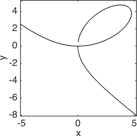
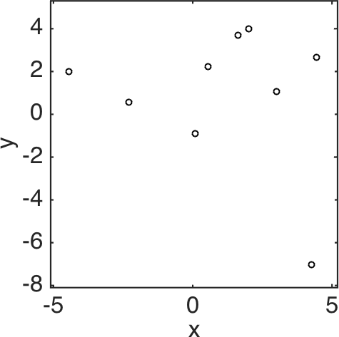
(a)	(b)
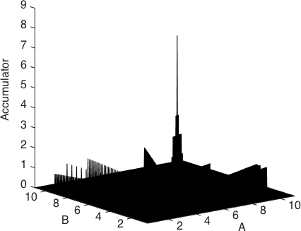
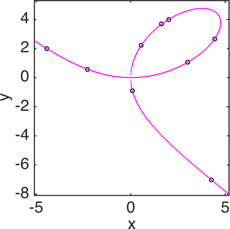
(c)	(d)

Figure 1: Recognition of the Descartes folium using $\nu_{\rm opt}=9$ points. The curve given by $a=3$, $b=1$, panel (a); $\nu_{\rm opt}$ points randomly sampled on the curve, panel (b); the accumulator function, panel (c); the recognized curve, in magenta, with sampled points superimposed, panel (d).

4.2 Robustness in presence of noisy background

In this paragraph we present the results concerning the robustness in presence of a very noisy background around the selected curves as above. For each curve we build a database made of $N_{1}+N_{2}$ points where $N_{1}=\nu_{\rm opt}$ points (dataset points, from now on) satisfy the curve equation, and $N_{2}$ points (noise points, from now on) are randomly picked up on the image plane according to a uniform distribution. We test different levels of background noise ($99\%$, $95\%$, $90\%$, $85\%$, $80\%$), considering

$$\frac{N_{2}}{\nu_{\rm opt}+N_{2}}=\frac{x}{100},$$ (8)

where $x=99,95,90,85,80$. For the four given curves, the values of $N_{1}$ and $N_{2}$ and the total number $N=N_{1}+N_{2}$ of Hough transforms, which depends on the background noise level, are summarized in Table 2. Let us remark that the quantity $N$ is definitely lower than the corresponding one employed in [2]. For instance, in the case of background noise at $99\%$ (the only case made explicit in [2]), here we employ $900$ points for the Descartes Folium and the elliptic curve, $1400$ for the quartic curve with triple point, and $1300$ for the quartic curve with tacnode, versus $10000$ for the Descartes Folium, $15800$ for the elliptic curve, $10000$ for the quartic curve with triple point, and $5000$ for the quartic curve with tacnode as reported in Table 2 of [2].

		Noise level
		$99\%$		$95\%$		$90\%$		$85\%$		$80\%$
Family of curves	$N_{1}$	$N_{2}$	$N$	$N_{2}$	$N$	$N_{2}$	$N$	$N_{2}$	$N$	$N_{2}$	$N$
Descartes Folium	$9$	$891$	$900$	$171$	$180$	$81$	$90$	$51$	$60$	$36$	$45$
Elliptic curve	$9$	$891$	$900$	$171$	$180$	$81$	$90$	$51$	$60$	$36$	$45$
Quartic curve with triple point	$14$	$1386$	$1400$	$266$	$280$	$126$	$140$	$80$	$94$	$56$	$70$
Quartic curve with tacnode	$13$	$1287$	$1300$	$247$	$260$	$117$	$130$	$74$	$87$	$52$	$65$

Table 2: Number of points used in the robustness test for the Hough transform recognition method: $N_{1}=\nu_{\rm opt}$, the number of points on each curve, $N_{2}$, the number of background noise points satisfying the condition $\frac{N_{2}}{\nu_{\rm opt}+N_{2}}=\frac{x}{100}$ in the case of noise $\frac{x}{100}=99\%,95\%,90\%,85\%,80\%$, and $N=N_{1}+N_{2}$, the total number of points.

We repeated the experiments for $100$ runs, randomly extracting the $N_{1}$ points on the curve and the $N_{2}$ background noise points. In Table 3 we show the number of runs (out of $100$) in which the method correctly recognizes the parameters, while in Table 4 we show the average distance and the corresponding standard deviation between the pair of exact parameters and the recognized ones.

In Figure 2 we represent the recognized curves in $100$ runs when the background noise is at $99\%$. The colors of the curves are associated to their repetition rates, as follows. Cyan, from $2\%$ to $3\%$; green, from $3\%$ to $5\%$; yellow, from $5\%$ to $10\%$; orange, from $10\%$ to $20\%$; red, from $20\%$ to $50\%$; magenta, higher than $50\%$. In Figure 3 we show the recognized curves with background noise at $95\%$ level: almost all the recognitions are perfect with the exception of the curve shown in panel (c) where in $3\%$ of the cases at most, a profile not perfectly matching the given curve is found. In Figure 4 we show the recognized quartic curve with a triple point when the background noise is decreased to $90\%$ (the only case which seemed critical at the previously considered noise level).

As previously stated, in all the trials the cyan and green curves occurred with a repetition rate lower than $5\%$ and for this reason we can assume they are not stable, reliable estimations of the real parameters. Further, as experimentally shown in Tables 3 and 4, the results look stable for background noise starting from $90\%$, so we omit the tables and figures corresponding to the $x=80,85$ cases.

Family of curves	Background noise level
	$99\%$	$95\%$	$90\%$
Descartes Folium	$41\%$	$100\%$	$100\%$
Elliptic curve	$100\%$	$100\%$	$100\%$
Quartic curve with triple point	$14\%$	$98\%$	$100\%$
Quartic curve with tacnode	$92\%$	$100\%$	$100\%$

Table 3: Percentage of runs (out of 100) in which we exactly recognize the parameters for the four curves and for different levels of background noise.

Family of curves	Background noise level
	$99\%$	$95\%$	$90\%$
Descartes Folium	$0.6\pm 0.6$	$0\pm 0$	$0\pm 0$
Elliptic curve	$0\pm 0$	$0\pm 0$	$0\pm 0$
Quartic curve with triple point	$0.4\pm 0.4$	$0.0002\pm 0.0014$	$0\pm 0$
Quartic curve with tacnode	$0.2\pm 1.0$	$0\pm 0$	$0\pm 0$

Table 4: Average distances, and corresponding standard deviations, between the pair of exact parameters and the recognized ones for the four curves and for different levels of background noise.

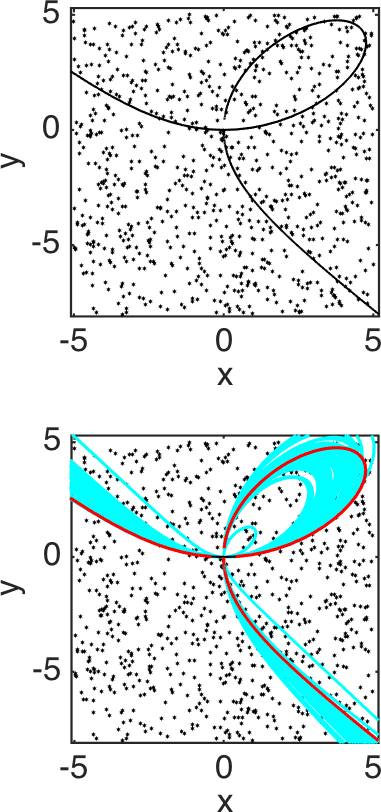
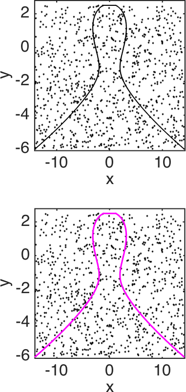
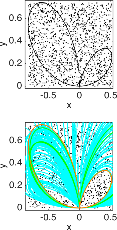
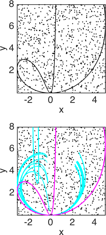
(a)	(b)	(c)	(d)

Figure 2: Recognition of the Descartes Folium, panel (a), the elliptic curve, panel (b), the quartic curve with a triple point, panel (c), and the quartic curve with tacnode, panel (d), when embedded in a noisy background ($99\%$ of background noise points). For each case, and for a run out of the $100$ we considered, the first row represents the noise points (dots) and the given curve (solid), whereas the second row represents the noise points (dots) and the recognized curves (solid). The colors of the curves are associated to their repetition rates.

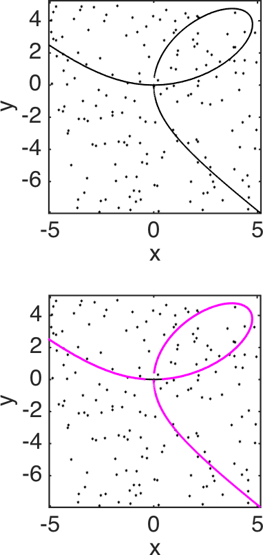
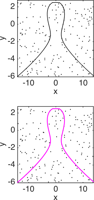
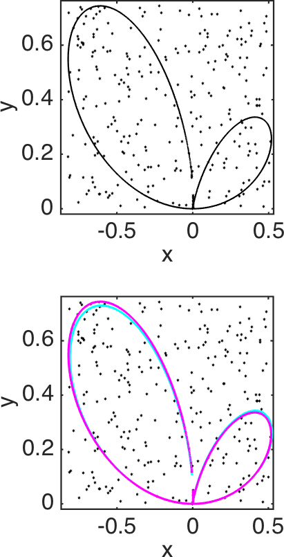
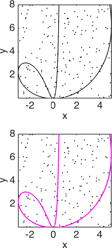
(a)	(b)	(c)	(d)

Figure 3: Recognition of the Descartes Folium, panel (a), the elliptic curve, panel (b), the quartic curve with a triple point, panel (c), and the quartic curve with tacnode, panel (d), when embedded in a noisy background ($95\%$ of background noise points). For a run out of the $100$ we considered, the first row in each panel represents the noise points (dots), and the given curve (solid), whereas the second row represents the noise points (dots) and the recognized curves (solid). The magenta color of the curves means that their repetition rates are higher than $50\%$; in the case of the quartic with a triple point a cyan colored curve occurs as well (repetition rate from 2% to 3%).

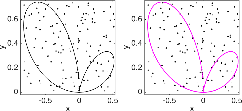
Figure 4: Recognition of the quartic curve with a triple point, when embedded in a noisy background ($90\%$ of background noise points). Left panel: noise points (dots) (again for a run out of the $100$ we considered) and given curve (solid). Right panel: noise points (dots) and recognized curves (solid); the only color present in the panel (magenta) means that the repetition rate of the recognized curve is higher than $50\%$.

4.2.1 The case of the Descartes Folium

Tables 3 and 4 show that the recognition of the Descartes Folium is not completely reliable in the case of $99\%$ of background noise points. In [2], the recognition of the Descartes Folium with this background noise percentage was performed by using a total of $10000$ points $N_{2}=9900$ and $N_{1}=100$. Here we want to investigate how much we need to increase the $N_{1}$ value (from the initial $\nu_{{\rm opt}}$ value), and consequently the total number of points $N$, in order to have perfectly reliable recognitions even with $99\%$ of background noise points. We employ the same procedure as in the previous section. In Table 5 we show the number of runs (out of $100$) in which the method correctly recognizes the parameters of the Descartes Folium for different values of $N_{1}$, and then $N$. As we can see it is necessary to increase the $N_{1}$ value to $25$ in order to have a $100\%$ of correct recognitions in presence of $99\%$ of background noise points.

$N_{1}\geq\nu_{{\rm opt}}$	$N_{2}$	$N=N_{1}+N_{2}$	Percentage of runs
$9$	$891$	$900$	$41\%$
$15$	$1485$	$1500$	$92\%$
$20$	$1980$	$2000$	$97\%$
$25$	$2475$	$2500$	$100\%$

Table 5: Percentage of runs (out of 100) in which we exactly recognize the parameters for the Descartes Folium with $99\%$ of background noise points by increasing the number of points selected on the given curve with respect to the bound value $\nu_{{\rm opt}}=9$.

4.3 Robustness against random perturbation of points’ locations

Here we validate the robustness of the recognition method against random perturbations of the location of points on the curves, following the procedure already employed in [2, p. 405], and by using $\nu_{\rm opt}$ instead of $N=100$. The procedure is repeated for $100$ runs. More specifically, for each of the four families of curves as above:

1. Take $\nu_{\rm opt}$ points randomly on the curve, according to a uniform distribution.

2. Repeat for $100$ different runs the steps:

   1. perturb each coordinate of each point $(x,y)$ in this database by means of a Gaussian distribution $\mathcal{N}(0,\sigma^{2})$ with zero mean and standard deviation $\sigma$;

   2. apply the recognition algorithm and determine the pair of parameters characterizing the curve;

   3. In the parameter space, compute the Euclidean distance between the computed parameter pair and the exact one.

3. Compute the average value, and corresponding standard deviations, of the $100$ distances computed in step $2$(c).

4. Repeat the procedure from step $2$ for a different value of the standard deviation in the Gaussian distribution.

The results of this test are shown in Table 6. First, note that the recognition capability of the method in the case of random perturbations of the points’ locations on the curve deteriorates differently for the four curves: the elliptic curve and the quartic curve with tacnode show poor results starting from $\sigma=0.04$, while in the case of the other curves the algorithm performs relatively well even with $\sigma=0.15$. Next, we also look at the number of exact recognitions of the four given curves. The Descartes Folium behaves well for small values of $\sigma$, with exact recognition rates of $24\%$, $12\%$, $4\%$, $1\%$, $1\%$ for $\sigma=0.01,~{}0.02,~{}0.04,~{}0.05,~{}0.06$, respectively. These values may seem low but, if combined with those shown in Table 6, they indicate that even when not perfect the recognition is still very accurate. The elliptic curve case shows high rates of exact recognition ($89\%$, $44\%$, $14\%$, $10\%$, $4\%$, $1\%$ for $\sigma=0.01,~{}0.02,~{}0.04,~{}0.05,~{}0.06,~{}0.1$, respectively), but, at the same time, when the recognition goes wrong, the parameters values we found rather differ from $a=-4$, $b=7$, also in the case of small values of the standard deviation $\sigma$, thus justifying the overall non-optimal behavior shown in Table 6. In the case of the quartic curve with triple point, we never find the exact parameters $a=\frac{1}{5}$, $b=\frac{1}{2}$, but we get parameters values rather close to them for all the considered values of $\sigma$. The quartic curve with tacnode presents an $11\%$ rate of exact recognition for $\sigma=0.01$, while for higher values of $\sigma$ the recognition of the exact parameters $a=1$, $b=8$ systematically fails.

	Family of curves
Standard	Descartes	Elliptic	Quartic curve	Quartic curve
deviation $\sigma$	Folium	curve	with triple point	with tacnode
$0.01$	$0.08\pm 0.1$	$0.2\pm 0.7$	$0.02\pm 0.03$	$0.1\pm 0.1$
$0.02$	$0.2\pm 0.6$	$0.6\pm 1.6$	$0.06\pm 0.09$	$0.4\pm 0.8$
$0.04$	$0.4\pm 0.7$	$1.1\pm 1.9$	$0.4\pm 0.6$	$0.8\pm 1.2$
$0.05$	$0.4\pm 0.6$	$1.5\pm 2.4$	$0.5\pm 0.6$	$1.0\pm 1.3$
$0.06$	$0.3\pm 0.5$	$2.4\pm 3.1$	$0.5\pm 0.6$	$1.3\pm 1.7$
$0.08$	$0.5\pm 0.6$	$2.6\pm 3.2$	$0.6\pm 0.8$	$1.8\pm 1.8$
$0.1$	$0.4\pm 0.4$	$3.4\pm 3.4$	$0.7\pm 0.7$	$2.2\pm 2.2$
$0.15$	$0.4\pm 0.4$	$4.0\pm 3.2$	$0.7\pm 0.6$	$2.9\pm$2.1

Table 6: Results of a test assessing the robustness of the recognition method with respect to random perturbations of points’ locations on the four curves: the rows contain the average distance, and corresponding standard deviation, between the pair of the exact parameters and the pair of the recognized ones.

In Figure 5 we summarize the recognized curves in the $100$ runs when $\sigma=0.02$ (central column) and $\sigma=0.04$ (right column). The colors of the curves are associated with the repetition rates as above. The repetition rates of the curves are rather low in most of the cases (the cyan color is associated with a repetition rate between the $2\%$ and the $3\%$), except for the elliptic curve, in which the given curve associated to $a=-4$, $b=7$ has a repetition rate from $20\%$ to $50\%$ (red color) for $\sigma=0.02$ and a repetition rate from $10\%$ to $20\%$ (orange color) for $\sigma=0.04$. We note that the quartic curve with tacnode shows a higher average distance between the pair of the exact parameters $a=1$, $b=8$ and the pairs of the recognized parameters if compared with the other curves; however, the graphs of the curves associated to the recognized parameters look “reasonably close” to that of the given quartic curve (see Figure 5, last row).

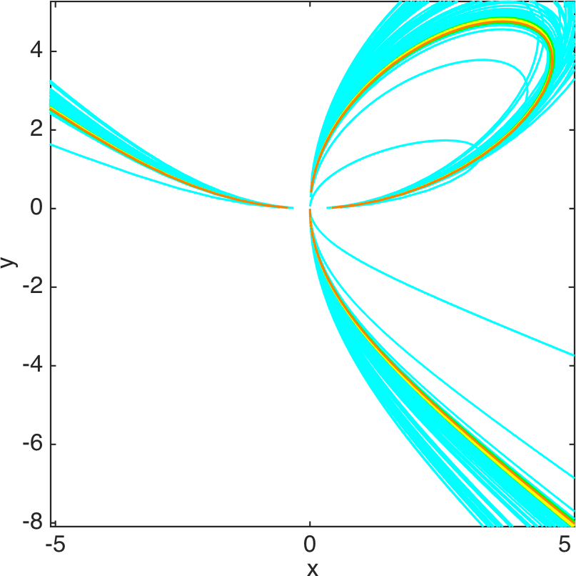
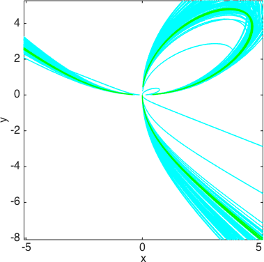
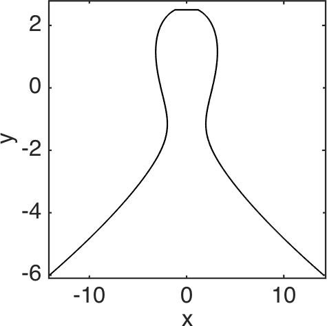
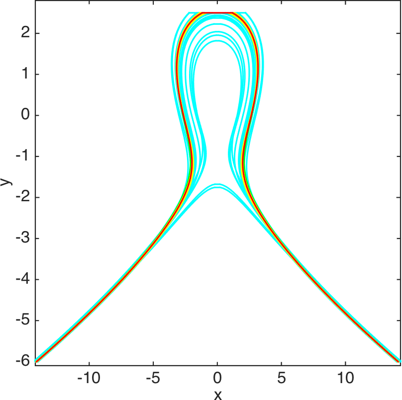
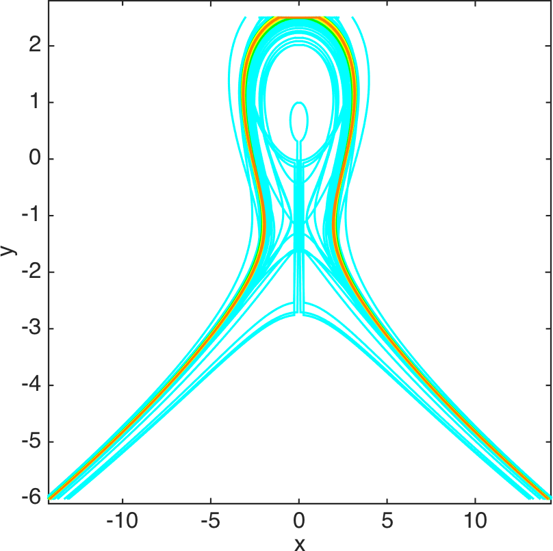
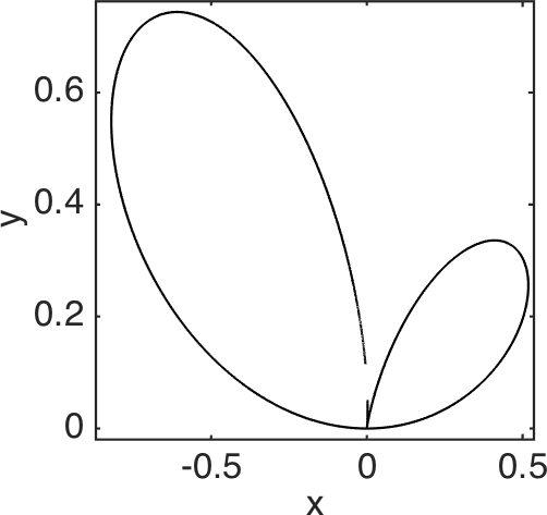
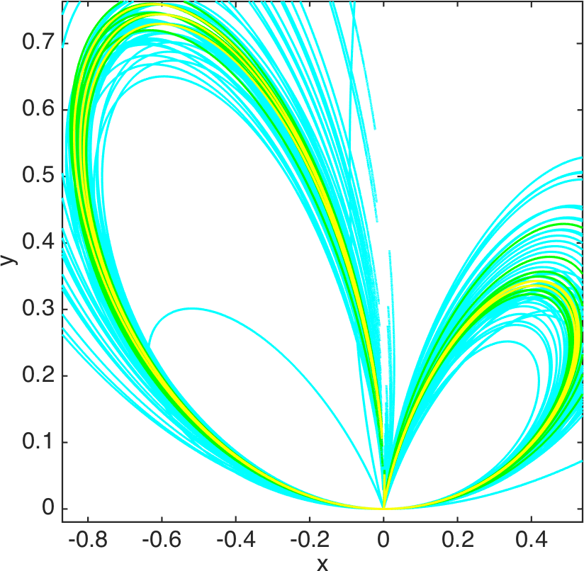
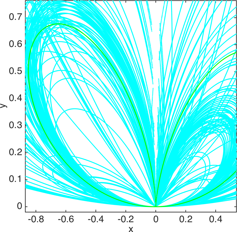
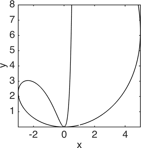
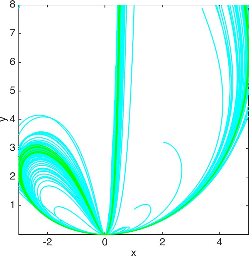
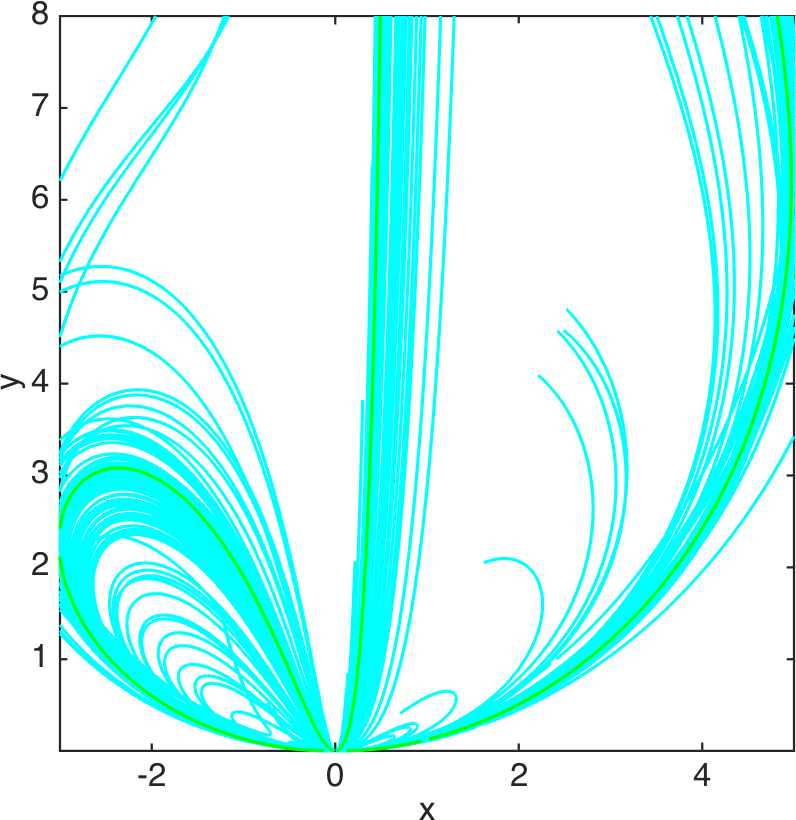
Figure 5: The four given curves (left column) and their recognition when the locations of $\nu_{\rm opt}$ points randomly taken on the curves are perturbed by using a $\mathcal{N}(0,\sigma^{2})$ distribution where $\sigma=0.02$ (central column) and $\sigma=0.04$ (right column). The colors of the curves are associated to their repetition rates: from $2\%$ to $3\%$: cyan; from $3\%$ to $5\%$: green; from $5\%$ to $10\%$: yellow; from $10\%$ to $20\%$: orange; from $20\%$ to $50\%$: red.

4.4 Computational cost

The use of bound $\nu_{\rm{opt}}$ allows us to recognize the curve by using a relatively small number of “good” points. Here we assess the reduction of the computational cost when a small set of points is considered: for each family of curves, we measured the time needed to go through the recognition procedure in the case of $99\%$ background noise (the same percentage as in [2]) with the same number of points as in Section 4.2 and in [2]. The results, provided in Table 7, show a significant decrease in terms of time for all the families of curves we considered here with a minimum factor $3.7$ and a maximum $21.2$.

Family of curves	$N$	time [s]	$N$	time [s]
Descartes Folium	$900$	$1.5$	$10000$	$12.7$
Elliptic curve	$900$	$5.1$	$15800$	$108.5$
Quartic curve with triple point	$1400$	$3.5$	$10000$	$21.5$
Quartic curve with tacnode	$1300$	$7.9$	$5000$	$29.6$

Table 7: Comparison between computational times (in seconds) for the recognition algorithm, with background noise level at $99\%$, when the number of employed points is $N=\nu_{\rm opt}+N_{2}$ (first two columns), and when $N$ is as in [2, Section 6] (third and fourth columns).

5 Conclusions

We propose a finite bound, $\nu_{\rm opt}$ (see Proposition 2.4), for the number of transforms to be considered in the accumulator function step of the recognition algorithm on which the Hough transform technique is based. Such a bound looks quite reliable and definitely of potential interest to reduce the computational burden associated to the accumulator function computation and optimization. In particular, we obtain quite effective results when the curves are embedded in a noisy background not exceeding $95\%$ (figures 3 and 4). E.g., for background noise at $95\%$, with a data set of $N_{1}=\nu_{\rm opt}$ and $N_{2}=\frac{95}{5}\nu_{\rm opt}=19\nu_{\rm opt}$ noise points (see relation (8)), we recognize the curve by considering a total of

$$N=N_{1}+N_{2}=20\nu_{\rm opt}\approx 20d^{2}$$

Hough transforms, where $d$ denotes the degree of the curves from the family. Note that in [2, Section 6, Table I] the recognition is extremely effective even when the curves are embedded in a noisy background at $99\%$, but using a number $N$ of total Hough transforms which approximately ranges from $5\times 10^{3}$ to $15\times 10^{3}$.

Not surprisingly, the results are not as good against random perturbations of points’ locations on the curves. In the case of the quartic curve with a tacnode (the only one explicitly shown in [2, Table 2]), we may for instance note that by using $N_{1}=\nu_{\rm opt}=13$ (instead of $N_{1}=100$) we need a standard deviation $\sigma=0.01$ (instead of $0.04$) to get the same average distance and corresponding standard deviation $0.1\pm 0.1$. Even if our results get worse as $\sigma$ increases, they deserve to be noted.

Appendix A An algebraic bound

We keep the notation and assumptions as in the previous sections. A better understanding of the behavior of equations defining the Hough transforms in the parameter space leads to a refinement of Proposition 2.4 (see Proposition A.4).

To begin with, let’s add some comments on the degree and dimension of the Hough transform of points in ${\mathbb{A}}_{{\bm{x}}}^{n}(K)$, $K={\mathbb{R}},{\mathbb{C}}$.

Clearly, there exists a Zariski open set ${\mathcal{U}}_{1}\subseteq{\mathbb{A}}_{{\bm{x}}}^{n}(K)$ such that, for each point $p\in{\mathcal{U}}_{1}$, the Hough transform $\Gamma_{p}({\mathcal{F}}):f_{p}(\bm{\Lambda})=0$ of $p$ is a zero locus of a polynomial of degree $h$ (not depending on $p$) in the parameter space. Since the Euclidean topology is finer than the Zariski topology, this holds true on a Euclidean open set ${\mathcal{U}}_{1}$ as well. If $K={\mathbb{C}}$, the Hough transform $\Gamma_{p}({\mathcal{F}})$ is a hypersurface. If $K={\mathbb{R}}$, then $\Gamma_{p}(\mathcal{F})$ is $(t-1)$-dimensional if and only if the polynomial $f_{p}=f_{p}(\bm{\Lambda})\in{\mathbb{R}}[\Lambda_{1},\ldots,\Lambda_{t}]$ has a non-singular zero in $\bm{\lambda}\in{\mathbb{R}}^{t}$, that is, the gradient $\Big{(}\frac{\partial f_{p}}{\partial\Lambda_{1}}(\bm{\lambda}),\ldots,\frac{\partial f_{p}}{\partial\Lambda_{t}}(\bm{\lambda})\Big{)}\neq 0$ (see again [4, Theorem 4.5.1] for details and equivalent conditions). A standard argument then shows that there exists a Euclidean open set ${\mathcal{U}}_{2}\subseteq{\mathbb{A}}_{{\bm{x}}}^{n}({\mathbb{R}})$ such that for each point $p\in{\mathcal{U}}_{2}$ the Hough transform $\Gamma_{p}({\mathcal{F}})$ is a hypersurface in ${\mathbb{A}}_{\bm{\Lambda}}^{t}({\mathbb{R}})$ (for instance, see [19] for details). Indeed, as a special case of a more general result (see [15, Proposition 2.25]), it holds true that the Hough transform $\Gamma_{p}(\mathcal{F})$ is $(t-1)$-dimensional for a generic point $p\in{\mathbb{A}}_{(x,y)}^{2}(K)$, if $K$ is a field. The above comments amount to conclude that, for each point $p$ varying in the Euclidean open set ${\mathcal{U}}_{1}\cap{\mathcal{U}}_{2}\subseteq{\mathbb{A}}_{{\bm{x}}}^{n}(K)$, the Hough transform $\Gamma_{p}({\mathcal{F}})$ is a hypersurface of given degree $h$ not depending on $p$. Following [19, Section 4] we then define the Hough transforms invariance degree open set as ${\mathcal{U}}_{1}$ if $K={\mathbb{C}}$ and ${\mathcal{U}}_{1}\cap{\mathcal{U}}_{2}$ if $K={\mathbb{R}}$.

From now on, we assume $n=2$. First, we note a fact we subsume in the sequel. Let ${\mathcal{B}}_{\rm aff}$ be the base locus associated to a family ${\mathcal{F}}=\{{\mathcal{C}}_{\bm{\lambda}}\}$ of curves (see Definition 2.1). Since clearly ${\mathcal{U}}_{1}\cap{\mathcal{B}}_{\rm aff}=\emptyset$, one has

$${\mathcal{C}}_{\bm{\lambda}}\cap{\mathcal{U}}_{1}\subseteq{\mathcal{C}}_{\bm{\lambda}}\setminus{\mathcal{B}}_{\rm aff}$$

for each curve ${\mathcal{C}}_{\bm{\lambda}}$ from the family.

Given a point $p=(x_{p},y_{p})$ in the image space, belonging to the invariance degree open set ${\mathcal{U}}_{1}\subset{\mathbb{A}}_{(x,y)}^{2}(K)$, write the polynomial $f_{p}(\bm{\Lambda})$, defining the Hough transform $\Gamma_{p}(\mathcal{F})$ of $p$, as

$$f_{p}(\bm{\Lambda})=\sum_{i+j=0}^{d}x_{p}^{i}y_{p}^{j}~{}g_{ij}(\bm{\Lambda})=\sum_{m_{1},\ldots,m_{t}}f_{m_{1},\ldots,m_{t}}(x_{p},y_{p})\Lambda_{1}^{m_{1}}\ldots\Lambda_{t}^{m_{t}}\in K[\bm{\Lambda}],$$ (9)

with $0\leq m_{1}+\cdots+m_{t}\leq h$, where $h$ is the degree of $f_{p}(\Lambda)$. Let $f_{p}(\bm{\Lambda})=f_{h}+\cdots+f_{0}$ be the decomposition of $f_{p}(\bm{\Lambda})$ into homogeneous components, where $f_{\alpha}\in K[\bm{\Lambda}]$ is homogeneous of degree $\alpha$, for $\alpha=0,\ldots,h$. Let $\Lambda_{0}$ be the new homogenizing coordinate. The homogenization of $f_{p}(\bm{\Lambda})$ with respect to $\Lambda_{0}$ is the polynomial $f_{p}(\bm{\Lambda})^{\hom}=f_{h}+f_{h-1}\Lambda_{0}+\cdots+f_{0}\Lambda_{0}^{h}\in K[\Lambda_{0},\bm{\Lambda}]$.

We order the monomials of the polynomial ring $K[\Lambda_{0},\Lambda_{1},\ldots,\Lambda_{t}]$; for instance, according to the degree-lexicographic order with $\Lambda_{t}<\cdots<\Lambda_{0}$ (see [8, p. 48]). Let’s give some definitions.

Definition A.1.

We say that the set ${\mathscr{S}}=\bigcup_{p\in{\mathcal{U}}_{1}}\big{(}{\rm Supp}(f_{p}(\bm{\Lambda}))^{\rm hom}\big{)}$ is the generic ordered support according to the fixed ordering. We also write $s:=\#{\mathscr{S}}$.

Definition A.2.

Take a finite set of points $p_{1},\ldots,p_{\nu}$ in the image space, belonging to the invariance degree open set ${\mathcal{U}}_{1}$, and let $M(p_{1},\ldots,p_{\nu};{\mathcal{F}})\in{\rm Mat}_{\nu\times s}(K)$ be the matrix whose $j$-th row consists of the coefficients of the polynomial $f_{p_{j}}(\bm{\Lambda})^{\hom}$ ordered according to Definition A.1. We say that $M(p_{1},\ldots,p_{\nu};{\mathcal{F}})$ is the HT-matrix associated to the points $p_{1},\ldots,p_{\nu}$ with respect to the family ${\mathcal{F}}$. We denote by $\varrho(M(p_{1},\ldots,p_{\nu};{\mathcal{F}}))$ its rank.

We are interested to find a minimal set of generators of the ideal $\big{(}f_{p_{1}}(\bm{\Lambda}),\ldots,f_{p_{\nu}}(\bm{\Lambda})\big{)}$ in $K(\bm{\Lambda}]$. To this purpose, just for technical reasons we pass to the homogenization, then working in $K[\Lambda_{0},\bm{\Lambda}]$. The following general fact (not involving specific curves from the family) achieves our goal.

Proposition–Definition A.3.

Notation as above. Let ${\mathcal{F}}$ be a family of curves in ${\mathbb{A}}_{(x,y)}^{2}(K)$. Let ${\mathscr{I}}=\{p_{1},\ldots,p_{\nu}\}$ be a set of distinct points belonging to the invariance degree open set ${\mathcal{U}}_{1}\subset{\mathbb{A}}_{(x,y)}^{2}(K)$. Let ${\mathscr{T}}_{\nu}:=\bigcap_{i=1,\ldots,\nu}\Gamma_{p_{j}}(\mathcal{F})$. Consider the smallest positive integer $\nu_{\rm best}:=\nu_{\rm best}(p_{1},\ldots,p_{\nu})\leq\nu$ defined by the condition that there exist indices $1\leq j_{1}\leq\cdots\leq j_{\nu_{\rm best}}\leq\nu$ such that

$$\big{(}f_{p_{1}}(\bm{\Lambda})^{\hom},\ldots,f_{p_{\nu}}(\bm{\Lambda})^{\hom}\big{)}=\big{(}f_{p_{j_{1}}}(\bm{\Lambda})^{\hom},\ldots,f_{p_{j_{\nu_{\rm best}}}}(\bm{\Lambda})^{\hom}\big{)},$$

and set ${\mathscr{T}}_{\rm best}:=\Gamma_{p_{j_{1}}}(\mathcal{F})\cap\ldots\cap\Gamma_{p_{j_{\nu_{\rm best}}}}(\mathcal{F})$. Then,

1. $\nu_{\rm best}=\varrho\big{(}M(p_{1},\ldots,p_{\nu};{\mathcal{F}})\big{)}$;

2. ${\mathscr{T}}_{\nu}={\mathscr{T}}_{\rm best}$.

Proof.

To prove statement $1)$, set $M:=M(p_{1},\ldots,p_{\nu};{\mathcal{F}})$ and let us first show $\nu_{\rm best}\leq\varrho(M)$. If $\varrho(M)=\nu$, then obviously $\nu_{\rm best}\leq\varrho(M)$, so we assume that $\varrho(M)<\nu$. We know that there exist $\varrho(M)$ rows of $M$ which are linearly independent and span the vectors space generated by all the rows of $M$. Up to renaming, we can assume that these are the first $\varrho(M)$ rows of $M$. Pick the $j$-th row $R_{j}$ of $M$ with $j>\varrho(M)$. Then $R_{j}$ can be written as a linear combination of the rows $R_{1},\ldots,R_{\varrho(M)}$. That is (denoting for simplicity $f_{p_{j}}:=f_{p_{j}}(\bm{\Lambda})$, $j=1,\ldots,\nu$), there exist $\alpha_{1}^{j},\ldots,\alpha_{\varrho(M)}^{j}\in K$ such that $R_{j}=\alpha_{1}^{j}R_{1}+\cdots+\alpha_{\varrho(M)}^{j}R_{\varrho(M)}$. This implies that $f_{p_{j}}^{\hom}=\alpha_{1}^{j}f_{p_{1}}^{\hom}+\cdots+\alpha_{\varrho(M)}^{j}f_{p_{\varrho(M)}}^{\hom}$, so that $f_{p_{j}}^{\hom}\in\big{(}f_{p_{1}}^{\hom},\ldots,f_{p_{\varrho(M)}}^{\hom}\big{)}$. Since this holds true for each $j>\varrho(M)$, we have

$$\big{(}f_{p_{1}}^{\hom},\ldots,f_{p_{\nu}}^{\hom}\big{)}\subseteq\big{(}f_{p_{1}}^{\hom},\ldots,f_{p_{\varrho(M)}}^{\hom}\big{)},$$

which implies $\big{(}f_{p_{1}}^{\hom},\ldots,f_{p_{\nu}}^{\hom}\big{)}=\big{(}f_{p_{1}}^{\hom},\ldots,f_{p_{\varrho(M)}}^{\hom}\big{)}$. We then conclude that $\nu_{\rm best}\leq\varrho(M)$ by the minimality of $\nu_{\rm best}$.

To show the converse, and up to renaming, let $f_{p_{1}}^{\hom},\ldots,f_{p_{\nu_{\rm best}}}^{\hom}$ be the generators of $\big{(}f_{p_{1}}^{\hom},\ldots,f_{p_{\nu}}^{\hom}\big{)}$. If $\nu_{\rm best}=\nu$ there is nothing to prove, so we assume that $\nu_{\rm best}<\nu$. For each $f_{p_{j}}^{\hom}$ with $j>\nu_{\rm best}$ we have $f_{p_{j}}^{\hom}\in\big{(}f_{p_{1}}^{\hom},\ldots,f_{p_{\nu_{\rm best}}}^{\hom}\big{)}$, that is, there exist polynomials $h_{i}^{j}$, $j=1,\ldots,\nu$, $i=1,\ldots,\nu_{\rm best}$, such that

$$f_{p_{j}}^{\hom}=h_{1}^{j}f_{p_{1}}^{\hom}+\cdots+h_{\nu_{\rm best}}^{j}f_{p_{\nu_{\rm best}}}^{\hom}.$$ (10)

Since $f_{p_{j}}^{\hom}$ and $f_{p_{1}}^{\hom},\ldots,f_{p_{\nu_{\rm best}}}^{\hom}$ are homogeneous polynomials of the same degree it follows that the $h_{i}^{j}$’s are homogeneous of degree zero, that is, $h_{i}^{j}\in K$. Thus, equality (10) is equivalent to say that each row $R_{j}$ of $M$ is a linear combination of $R_{1},\ldots,R_{\nu_{\rm best}}$. The conclusion $\varrho(M)\leq\nu_{\rm best}$ then immediately follows.

As to statement $2)$, consider the ideal $(f_{p_{1}}(\bm{\Lambda}),\ldots,f_{p_{\nu}}(\bm{\Lambda}))$ in $K[\bm{\Lambda}]$. We want to prove that there exist indices $j_{1},\ldots,j_{\rm\nu_{\rm best}}$, $1\leq j_{1}<\cdots<j_{\rm\nu_{\rm best}}\leq\nu$, such that

$$(f_{p_{1}}(\bm{\Lambda}),\ldots,f_{p_{\nu}}(\bm{\Lambda}))=\big{(}f_{p_{j_{1}}}(\bm{\Lambda}),\ldots,f_{p_{j_{\rm\nu_{\rm best}}}}(\bm{\Lambda})\big{)}.$$

The inclusion “$\supseteq$” is obvious, so we only have to prove the converse inclusion “$\subseteq$”. By definition of $\nu_{\rm best}$, we know that there are indices $1\leq j_{1}<\cdots<j_{\rm\nu_{\rm best}}\leq\nu$, such that

$$(f_{p_{1}}^{\rm hom}(\bm{\Lambda}),\ldots,f_{p_{\nu}}^{\rm hom}(\bm{\Lambda})) = \big{(}f_{p_{j_{1}}}^{\rm hom}(\bm{\Lambda}),\ldots,f_{p_{j_{\rm\nu_{\rm best}}}}^{\rm hom}(\bm{\Lambda})\big{)}$$

$$\subseteq \big{(}f_{p_{j_{1}}}(\bm{\Lambda}),\ldots,f_{p_{j_{\rm\nu_{\rm best}}}}(\bm{\Lambda})\big{)}^{\rm hom},$$

where the last inclusion follows by definition of ideal homogenization (see [11, Definition 4.3.4]). Passing to the dehomogenization, we get (see [11, Proposition 4.3.12])

$$(f_{p_{1}}^{\rm hom}(\bm{\Lambda}),\ldots,f_{p_{\nu}}^{\rm hom}(\bm{\Lambda}))^{\rm deh} = \big{(}f_{p_{j_{1}}}^{\rm hom}(\bm{\Lambda}),\ldots,f_{p_{j_{\rm\nu_{\rm best}}}}^{\rm hom}(\bm{\Lambda})\big{)}^{\rm deh}$$

$$\subseteq \Big{(}\big{(}f_{p_{j_{1}}}(\bm{\Lambda}),\ldots,f_{p_{j_{\rm\nu_{\rm best}}}}(\bm{\Lambda})\big{)}^{\rm hom}\Big{)}^{\rm deh}$$

$$= \big{(}f_{p_{j_{1}}}(\bm{\Lambda}),\ldots,f_{p_{j_{\rm\nu_{\rm best}}}}(\bm{\Lambda})\big{)},$$

where the last equality is a consequence of [11, Proposition 4.3.5]. Since

$$(f_{p_{1}}^{\rm hom}(\bm{\Lambda}),\ldots,f_{p_{\nu}}^{\rm hom}(\bm{\Lambda}))^{\rm deh}=\big{(}f_{p_{1}}(\bm{\Lambda}),\ldots,f_{p_{\nu}}(\bm{\Lambda})\big{)},$$

(see [11, Corollary 4.3.8]), the claimed inclusion follows. Thus, we can conclude that

$${\mathscr{T}}_{\nu}=\Gamma_{p_{1}}(\mathcal{F})\cap\ldots\cap\Gamma_{p_{\nu}}(\mathcal{F})=\Gamma_{p_{j_{1}}}(\mathcal{F})\cap\ldots\cap\Gamma_{p_{j_{\nu_{\rm best}}}}(\mathcal{F}).$$

∎

Proposition A.4.

Notation as above. Let ${\mathcal{F}}=\{{\mathcal{C}}_{{\bm{\lambda}}}\}$ be a family of curves in ${\mathbb{A}}_{(x,y)}^{2}(K)$. Fix a curve ${\mathcal{C}}_{{\bm{\lambda}}}$ from the family, and take $\nu_{\rm opt}=d^{2}-\#{\mathcal{B}}({\mathbb{C}})+1$ distinct points $p_{1},\ldots,p_{\nu_{\rm opt}}$ on ${\mathcal{C}}_{{\bm{\lambda}}}\cap{\mathcal{U}}_{1}$. Let ${\mathscr{T}}=\cap_{p\in C_{\bm{\lambda}}}\Gamma_{p}(\mathcal{F})$ and let ${\mathscr{T}}_{\rm best}=\bigcap_{j=1,\ldots,\nu_{\rm best}}\Gamma_{p_{j}}(\mathcal{F})$. Then we have:

1. ${\mathcal{C}}_{{\bm{\lambda}}^{\prime}}={\mathcal{C}}_{{\bm{\lambda}}}$ for each ${\bm{\lambda}}^{\prime}\in{\mathscr{T}}_{\rm best}$.

2. ${\mathscr{T}}_{\rm best}={\mathscr{T}}$.

3. If the family ${\mathcal{F}}$ is Hough regular, then ${\mathscr{T}}_{\rm best}=\{{\bm{\lambda}}\}$.

Proof.

If $\nu_{\rm best}=d^{2}-\#{\mathcal{B}}({\mathbb{C}})+1$, the result simply follows from Proposition 2.4. Then we can assume that $\nu_{\rm best}=\varrho(M(p_{1},\dots,p_{\nu_{\rm opt}};{\mathcal{F}}))<d^{2}-\#{\mathcal{B}}({\mathbb{C}})+1$. Therefore, Proposition-Definition A.3(2) yields

$${\mathscr{T}}_{\rm opt}=\bigcap_{j=1,\ldots,\nu_{\rm opt}}\Gamma_{p_{j}}(\mathcal{F})=\bigcap_{j=1,\ldots,\nu_{\rm best}}\Gamma_{p_{j}}(\mathcal{F})={\mathscr{T}}_{\rm best}.$$

Thus, Proposition 2.4 applies again to conclude the proof. ∎

The following remark clarifies the relations between the bounds $\nu_{\rm opt}$ (see Proposition 2.4) and $\nu_{\rm best}$, as well as, for families $\mathcal{F}$ which are Hough regular, between them and the number of parameters $t$.

Remark A.5.

Assumptions and notation as in Proposition A.4. In fact, instead of $\nu_{\rm best}$, it is possible to use the easier computable bound

$$\nu_{\rm best}^{\prime}:=\min\{s-1,d^{2}-\#{\mathcal{B}}({\mathbb{C}})+1\},$$

with $s=\#{\mathscr{S}}$ as in Definition A.1. This follows from the fact that the points $p_{j}$, $j=1,\ldots,\nu_{\rm opt}$, lie on a given curve ${\mathcal{C}}_{\bm{\lambda}}$, $\bm{\lambda}=(\lambda_{1},\ldots,\lambda_{t})$, from the family ${\mathcal{F}}$, and consequently the $s$ columns of $M$ are linearly dependent. Precisely, recalling expression (9), one has

$$f_{p_{j}}(\bm{\Lambda})=\sum_{m_{1},\ldots,m_{t}}f_{m_{1},\ldots,m_{t}}(x_{p_{j}},y_{p_{j}})\Lambda_{1}^{m_{1}}\ldots\Lambda_{t}^{m_{t}}=0,$$

and the $j$-th row of $M$ is made up of the coefficients (ordered according to the fixed ordering) $f_{m_{1},\ldots,m_{t}}(x_{p_{j}},y_{p_{j}})$, for $j=1,\ldots,\nu_{\rm opt}$. In conclusion, we have the inequalities:

$$\nu_{\rm best}=\varrho(M)\leq\nu_{\rm best}^{\prime}=\min\{s-1,d^{2}-\#{\mathcal{B}}({\mathbb{C}})+1\}\leq\nu_{\rm opt}=d^{2}-\#{\mathcal{B}}({\mathbb{C}})+1.$$ (11)

Now, assume that the family $\mathcal{F}$ is Hough regular. Coming back to Subsection 1.1, consider the ideal

$$I=\big{(}f_{p_{1}}(\bm{\Lambda}),\ldots,f_{p_{h}}(\bm{\Lambda})\big{)}\subset K[\Lambda]$$

generated by the polynomials $f_{p}(\bm{\Lambda})$ defining the Hough transforms $\Gamma_{p}({\mathcal{F}})$, $p\in{\mathcal{C}}_{\lambda}$. Let $m$ be the minimal number of generators of $I$ in $K[\Lambda]$, so that, as we noted, $h\geq m$. Furthermore, such a number $m$ has to satisfy the lower bound $m\geq\textrm{codim}(I)$ (see [10] and also [8, Chapter 10]). By definition, $\textrm{codim}(I):=\textrm{dim}(K[\Lambda])-\textrm{dim}(K[\Lambda]/I)$. Since $\textrm{dim}(K[\Lambda])=t$ and $\textrm{dim}(K[\Lambda]/I)=0$ (this derives from the assumption that the family $\mathcal{F}$ is Hough regular, which implies that the ideal $I$ is zero-dimensional), it then follows $m\geq t$, whence $h\geq t$. Thus, in particular, relations (11) yield

$$\nu_{\rm opt}\geq\nu_{\rm best}\geq t.$$

$\Box$

We provide here some illustrative examples in the real case.

Example A.6.

(Curve of Lamet) Consider in $\mathbb{A}^{2}_{(x,y)}(\mathbb{R})$ the family ${\mathcal{F}}=\{{\mathcal{C}}_{a,b}\}$ of curves of degree $m$ of equation $\left(\frac{x}{a}\right)^{m}+\frac{y^{m}}{b}=1$, that is,

$$\mathcal{C}_{a,b}:bx^{m}+a^{m}y^{m}=a^{m}b,$$ (12)

for positive real numbers $a$, $b$. The curve of Lamet is clearly non-singular (even in the complex projective plane ${\mathbb{P}}^{2}({\mathbb{C}})$), and then of genus $\frac{(m-1)(m-2)}{2}$.

We further assume that the degree $m$ is even. As noted below, this assures the boundedness of the curve. (If $m$ is odd the curve is unbounded: think, for example, to the Fermat elliptic cubic of equation $x^{3}+y^{3}=1$.) Indeed, the knowledge of some basic facts about $p$-norms on $\mathbb{R}^{n}$ allows us to show that the curve of Lamet is contained in the rectangular region

$$\left\{(x,y)\in\mathbb{A}^{2}_{(x,y)}(\mathbb{R})\>\big{|}\>-a\leq x\leq a,\>-b^{1/m}\leq y\leq b^{1/m}\right\}.$$

Passing to homogeneous coordinates we have

$$\overline{{\mathcal{C}}_{a,b}}:bx_{0}^{m}+a^{m}x_{1}^{m}-a^{m}bx_{2}^{m}=0,$$

whence ${\mathcal{B}}({\mathbb{C}})=\{\emptyset\}$. In order to compute $\nu_{\rm best}$, note that for any point $p=(x_{p},y_{p})$ in the invariance degree open set ${\mathcal{U}}_{1}\subset{\mathbb{A}}_{(x,y)}^{2}({\mathbb{R}})$, the Hough transform is the $(m+1)$-degree curve $\Gamma_{p}({\mathcal{F}})$ in the parameter plane $\langle A,B\rangle$ of equation

$$f_{p}(A,B)=A^{m}B-y_{p}^{m}A^{m}-x_{p}^{m}B=0.$$

Therefore the bound from Proposition 2.4 becomes

$$\nu_{\rm opt}=d^{2}-\#{\mathcal{B}}({\mathbb{C}})+1=m^{2}+1.$$

For instance, in the case $m=4$, $\nu_{\rm opt}=17$. Thus, Proposition A.4 yields

$$\nu_{\rm best}\leq\min\{s-1,d^{2}-\#{\mathcal{B}}({\mathbb{C}})+1\}=\min\{2,17\}=2,$$

where $s:=\#{\mathscr{S}}$. To see that $\nu_{\rm best}=2$, take $17$ points $p_{\ell}=(x_{p_{\ell}},y_{p_{\ell}})$, $\ell=1,\ldots,17$, on the Lamet curve

$$\mathcal{C}_{a,b}:bx^{4}+a^{4}y^{4}-a^{4}b=0,$$

with $a$, $b$ fixed and the points belonging to the open set ${\mathcal{U}}_{1}$.

The coefficient of the maximum degree term of $f_{p}(A,B)$ equals $1$, so that it generates the whole ring ${\mathbb{R}}[A,B]$, that is, ${\mathcal{U}}_{1}={\mathbb{R}}^{2}$. Keeping the notation as in the proof of Proposition A.4, consider the (transpose of) HT-matrix $M$ associated to the set of points $\{p_{\ell}\}_{\ell=1,\ldots,17}$, that is,

$$M^{t}=\left(\begin{matrix}1&1&1&\cdots&1&\cdots&1\\ {\rule[-11.38109pt]{0.0pt}{28.45274pt}-y_{p_{1}}^{4}}&-y_{p_{2}}^{4}&-y_{p_{3}}^{4}&\cdots&-y_{p_{\ell}}^{4}&\cdots&-y_{p_{17}}^{4}\\ {\rule[-11.38109pt]{0.0pt}{28.45274pt}-x_{p_{1}}^{4}}&-x_{p_{2}}^{4}&-x_{p_{3}}^{4}&\cdots&-x_{p_{\ell}}^{4}&\cdots&-x_{p_{17}}^{4}\\ \end{matrix}\right)\in{\rm Mat}_{3\times 17}({\mathbb{R}}).$$

Compute, for $i,j,k\in\{1,\ldots,17\}$, $i\neq j\neq k$,

$$\left|\begin{matrix}1&1&1\\ {\rule[-11.38109pt]{0.0pt}{28.45274pt}-y_{p_{i}}^{4}}&-y_{p_{j}}^{4}&-y_{p_{k}}^{4}\\ {\rule[-11.38109pt]{0.0pt}{28.45274pt}-x_{p_{i}}^{4}}&-x_{p_{j}}^{4}&-x_{p_{k}}^{4}&\\ \end{matrix}\right| = \left|\begin{matrix}1&0&0\\ {\rule[-11.38109pt]{0.0pt}{28.45274pt}-y_{p_{i}}^{4}}&y_{p_{i}}^{4}-y_{p_{j}}^{4}&y_{p_{i}}^{4}-y_{p_{k}}^{4}\\ {\rule[-11.38109pt]{0.0pt}{28.45274pt}-x_{p_{i}}^{4}}&x_{p_{i}}^{4}-x_{p_{j}}^{4}&x_{p_{i}}^{4}-x_{p_{k}}^{4}&\\ \end{matrix}\right|$$

$$= (x_{p_{i}}^{4}-x_{p_{k}}^{4})(y_{p_{i}}^{4}-y_{p_{j}}^{4})-(x_{p_{i}}^{4}-x_{p_{j}}^{4})(y_{p_{i}}^{4}-y_{p_{k}}^{4})$$

$$= \frac{1}{b}(y_{p_{i}}^{4}-y_{p_{j}}^{4})(bx_{p_{i}}^{4}-bx_{p_{k}}^{4})-\frac{1}{b}(y_{p_{i}}^{4}-y_{p_{k}}^{4})(bx_{p_{i}}^{4}-bx_{p_{j}}^{4})$$

$$= \frac{1}{b}\big{[}(y_{p_{i}}^{4}-y_{p_{j}}^{4})(-a^{4}y_{p_{i}}^{4}+a^{4}y_{p_{k}}^{4})-(y_{p_{i}}^{4}-y_{p_{k}}^{4})(-a^{4}y_{p_{i}}^{4}+a^{4}y_{p_{j}}^{4})\big{]}$$

$$= \frac{a^{4}}{b}\big{[}(y_{p_{i}}^{4}-y_{p_{j}}^{4})(-y_{p_{i}}^{4}+y_{p_{k}}^{4})-(y_{p_{i}}^{4}-y_{p_{k}}^{4})(-y_{p_{i}}^{4}+y_{p_{j}}^{4})\big{]}=0,$$

to conclude that $\varrho(M)=\nu_{\rm best}=2$. $\Box$

Example A.7.

Consider in $\mathbb{A}^{2}_{(x,y)}(\mathbb{R})$ the family ${\mathcal{F}}=\{{\mathcal{C}}_{a,b}\}$ of conics of equation

$${\mathcal{C}}_{a,b}:a^{2}x^{2}+by+x=0,$$

for real parameters ${\bm{\lambda}}=(a,b)$. Passing to homogeneous coordinates we see that $\#{\mathcal{B}}({\mathbb{C}})=2$. Whence $\nu_{\rm opt}=d^{2}-\#{\mathcal{B}}({\mathbb{C}})+1=3$. For a general point $p=(x_{p},y_{p})$, the Hough transform is the conic of equation

$$f_{p}(A,B)=x_{p}^{2}A^{2}+y_{p}B+x_{p}=0,$$

so that $s=\#{\rm Supp}(f_{p}(A,B))=3=\nu_{\rm opt}$. Consider the three points $p_{1}=(1,-2)$, $p_{2}=(-1,0)$, $p_{3}=(-2,-2)$ on ${\mathcal{C}}_{1,1}$ and the polynomials $f_{p_{1}}(A,B)=A^{2}-2B+1$, $f_{p_{2}}(A,B)=A^{2}-1$, $f_{p_{3}}(A,B)=4A^{2}-2B-2$. The HT-matrix $M\in\rm{Mat}_{3\times 3}({\mathbb{R}})$ is

$$M=\left(\begin{matrix}1&-2&1\\ 1&0&-1\\ 4&-2&-2\end{matrix}\right),$$

whose rank is $\nu_{\rm{best}}=\varrho(M)=2$. We have ${\mathscr{T}}_{\rm best}=\Gamma_{p_{1}}({\mathcal{F}})\cap\Gamma_{p_{2}}({\mathcal{F}})=\{(1,1),(-1,1)\}$. (Note that $\Gamma_{p_{1}}({\mathcal{F}})$, $\Gamma_{p_{2}}({\mathcal{F}})$ have two more coinciding common points at infinity). The family ${\mathcal{F}}$ is not Hough regular unless $a>0$, in which case ${\mathscr{T}}_{\rm best}=\{(1,1)\}$. $\Box$

Although most of the times $\varrho(M)<d^{2}-\#{\mathcal{B}}({\mathbb{C}})+1$, so that $\nu_{\rm best}=\rho(M)$ there are also cases where the equality $\varrho(M)=d^{2}-\#{\mathcal{B}}({\mathbb{C}})+1$ holds true, as the following simple example shows.

Example A.8.

Consider in $\mathbb{A}^{2}_{(x,y)}(\mathbb{R})$ the family ${\mathcal{F}}=\{{\mathcal{C}}_{a,b,c}\}$ of lines of equation

$${\mathcal{C}}_{a,b,c}:ax+by+c=0,$$

for real parameters ${\bm{\lambda}}=(a,b,c)$. The polynomial defining the Hough transform of a general point $(x,y)$ is

$$f_{(x,y)}(A,B,C)=xA+yB+C\in{\mathbb{R}}[x,y][A,B,C],$$

having support ${\mathscr{S}}=\{A,B,C\}$. Then $s=3$, $d^{2}-\#{\mathcal{B}}({\mathbb{C}})+1=s-1=2$, whence $\nu_{\rm best}\leq 2$. Consider the two points $p_{1}=(0,-1)$, $p_{2}=(-1,0)$ on ${\mathcal{C}}_{1,1,1}$ , and the polynomials $f_{p_{1}}(A,B,C)=-B+C$, $f_{p_{2}}(A,B,C)=-A+C$. The HT-matrix $M\in\rm{Mat}_{2\times 3}({\mathbb{R}})$ is

$$M=\left(\begin{matrix}0&-1&1\\ -1&0&1\end{matrix}\right),$$

whose rank is $\nu_{\rm best}=\varrho(M)=2=\nu_{\rm opt}$. Then the set ${\mathscr{T}}_{\rm best}=\Gamma_{p_{1}}({\mathcal{F}})\cap\Gamma_{p_{2}}({\mathcal{F}})$ coincides with the line $\{(t,t,t)\>|\>t\in{\mathbb{R}}\}$ in the parameter space ${\mathbb{R}}^{3}=\langle A,B,C\rangle$. Clearly, ${\mathcal{C}}_{t,t,t}={\mathcal{C}}_{1,1,1}$ for each $t\in{\mathbb{R}}$, according to Proposition A.4(1).

The family ${\mathcal{F}}$ is not Hough regular, meeting the regularity property as soon as one of the parameters is fixed. For instance, letting $c=1$, we get the family of lines ${\mathcal{F}}^{\prime}=\{{\mathcal{C}}_{a,b}:ax+by+1=0\}$, and now ${\mathscr{T}}_{\rm best}=\Gamma_{p_{1}}({\mathcal{F}}^{\prime})\cap\Gamma_{p_{2}}({\mathcal{F}}^{\prime})=\{(1,1)\}$ with $p_{1}=(0,-1)$, $p_{2}=(-1,0)$ on ${\mathcal{C}}_{1,1}$.

Since the parameters are linear, the same conclusions follow from Lemma 2.2. $\Box$

Acknowledgments We would like to thank our friend and former colleague Annalisa Perasso, who previously effectively worked on the first stages of the project.

References

• [1] M.C. Beltrametti, E. Carletti, D. Gallarati and G. Monti Bragadin, Lectures on Curves, Surfaces and Projective Varieties—A Classical View of Algebraic Geometry, European Mathematical Society, Textbooks in Mathematics, 9. Translated by F. Sullivan. Zurich (2009).
• [2] M.C. Beltrametti, A.M. Massone and M. Piana, Hough transform of special classes of curves, SIAM J. Imaging Sci. 6(1), (2013), 391–412.
• [3] M.C. Beltrametti and L. Robbiano, An algebraic approach to Hough transforms, Journal of Algebra 371 (2012), 669–681.
• [4] J. Bochnak, M. Coste and M.-F. Roy, Real Algebraic Geometry, Ergeb. Math. Grenzgeb. 36, Springer-Verlag, Berlin Heidelberg (1998).
• [5] C. Campi, A. Perasso, M.C. Beltrametti, G. Sambuceti, A.M. Massone and M. Piana, HT BONE: A Graphical User Interface for the identification of bone profiles in CT images via extended Hough transform, Proc. SPIE 9784, Medical Imaging 2016: Image Processing, 978423 (March 21, 2016).
• [6] J. Canny, A Computational Approach to Edge Detection, IEEE Trans. Pattern Analysis and Machine Intelligence, 8(6) (1986), 679–698.
• [7] R.O. Duda and P.E. Hart, Use of the Hough transformation to detect lines and curves in pictures, Comm. ACM, 15, vol. 1 (1972), 11–15.
• [8] D. Einsenbud, Commutative Algebra—with a View Toward Algebraic Geometry, Graduate Texts in Mathematics, 150, Springer-Verlag, New York, Inc. (1995).
• [9] P.V.C. Hough, Method and means for recognizing complex patterns, US Patent 3069654, December 18, 1962.
• [10] C. Huneke and C. Raicu, Introduction to Uniformity in Commutative Algebra, in Commutative Algebra and Noncommutative Algebraic Geometry I: Expository Articles, MSRI Publications, Eds: D. Eisenbud, S. B. Iyengar, A.K. Singh, J.B. Stafford, M. Van den Bergh, vol. 67 (2015), 163–190.
• [11] M. Kreuzer and L. Robbiano, Computational Commutative Algebra 2, Springer-Verlag, Berlin (2005).
• [12] A.M. Massone, A. Perasso, C. Campi and M.C. Beltrametti, Profile detection in medical and astronomical imaging by means of the Hough transform of special classes of curves, J. Math. Imaging Vis. 51(2), (2015), 296–310.
• [13] A. Perasso, C. Campi, A.M. Massone and M.C. Beltrametti, Spinal canal and spinal marrow segmentation by means of the Hough Transform of special classes of curves”, Proceedings of the $18$-th Conference on Image Analysis and Processing, 7-11 September, 2015, Genova, Italy, Lecture Notes in Computer Sciences, Springer-Verlag.
• [14] G. Ricca, M.C. Beltrametti and A.M. Massone, Detecting curves of symmetry in images via Hough transform, Mathematics in Computer Sciences, Special Issue on Geometric Computation, 10(1) (2016), 179–205.
• [15] L. Robbiano, Hyperplane sections, Gröbner bases, and Hough transforms, Journal of Pure and Applied Algebra, 219 (2015), 2434–2448.
• [16] J.R. Sendra, F. Winkler and S. Pérez-Díaz, Rational Algebraic Curves—A Computer Algebra Approach, Algorithms and Computation in Mathematics, vol. 22, Springer-Verlag, Berlin (2008).
• [17] E.V. Shikin, Handbook and Atlas of Curves, CRC Press, Inc., Boca Raton (1995).
• [18] M. Torrente and M.C. Beltrametti, Almost-vanishing polynomials and an application to the Hough transform, J. Algebra Appl. 13(8), 1450057 (2014), 39 pp.
• [19] M. Torrente, M.C. Beltrametti and J.R. Sendra, Perturbation of polynomials and applications to the Hough transform, J. Algebra 486 (2017), 328–359.