A deterministic and computable Bernstein-von Mises theorem

Abstract

Bernstein-von Mises results (BvM) establish that the Laplace approximation is asymptotically correct in the large-data limit. However, these results are inappropriate for computational purposes since they only hold over most, and not all, datasets and involve hard-to-estimate constants. In this article, I present a new BvM theorem which bounds the Kullback-Leibler (KL) divergence between a fixed log-concave density $f\left(\boldsymbol{\theta}\right)$ and its Laplace approximation. The bound goes to $0$ as the higher-derivatives of $f\left(\boldsymbol{\theta}\right)$ tend to $0$ and $f\left(\boldsymbol{\theta}\right)$ becomes increasingly Gaussian. The classical BvM theorem in the IID large-data asymptote is recovered as a corollary.

Critically, this theorem further suggests a number of computable approximations of the KL divergence with the most promising being:

$$KL\left(g_{LAP},f\right)\approx\frac{1}{2}\text{Var}_{\boldsymbol{\theta}\sim g\left(\boldsymbol{\theta}\right)}\left(\log\left[f\left(\boldsymbol{\theta}\right)\right]-\log\left[g_{LAP}\left(\boldsymbol{\theta}\right)\right]\right)$$

An empirical investigation of these bounds in the logistic classification model reveals that these approximations are great surrogates for the KL divergence. This result, and future results of a similar nature, could provide a path towards rigorously controlling the error due to the Laplace approximation and more modern approximation methods.

Introduction

Bayesian inference is intrinsically plagued by computational problems due to the fact that its key object, the posterior distribution $f\left(\boldsymbol{\theta}|\text{Data}\right)$, is computationally hard to approximate. Solutions to this challenge can be roughly decomposed into two classes. Sampling methods, dating back to the famed Metropolis-Hastings algorithm (Metropolis et al. (1953); Hastings (1970)), provide a first possible solution: approximate the posterior using a large number of samples whose marginal distribution is the posterior distribution (Brooks et al. (2011)). Any expected value under the posterior can then be approximated using the corresponding empirical mean in the samples. A second solution is provided by Variational methods which aim to find the member of a parametric family $g\left(\boldsymbol{\theta};\lambda\right)$ which is the closest (in some sense) to the posterior $f\left(\boldsymbol{\theta}|\text{Data}\right)$ (Blei et al. (2017)). For example, the historical Laplace approximation (Laplace (1820)) proposes to approximate the posterior by a Gaussian centered at the Maximum A Posterior value while the more modern Gaussian Variational Approximation finds a Gaussian which minimizes the reverse Kullback-Leibler divergence (KL) (Opper and Archambeau (2009)). Computationally, the choice between the two corresponds to a trade-off between accuracy (the error of sampling methods typically converges at speed $s^{-1/2}$ where $s$ is the number of samples, while Variational methods will always have some residual error) and speed (Variational methods tend to quickly and cheaply find the best approximation; e.g. Nickisch and Rasmussen (2008)). Currently, Variational methods are furthermore held back by the fact that they are perceived to be unrigorous approximations due to the absence of results guaranteeing their precision.

One limit for which Variational methods are particularly interesting is for large datasets. Indeed, as the number of datapoints grows, sampling methods struggle computationally since the calculation of one additional sample requires a pass through the whole dataset (but see Bardenet et al. (2014); Chen et al. (2014); Maclaurin and Adams (2015); Bardenet et al. (2017) for modern attempts at tackling this issue). In contrast, Variational methods are still able to tackle these large datasets since they can leverage the computational prowess of optimization. For example, it is straightforward to solve an optimization problem while accessing only subsets (or batches) of the data at any one time, thus minimizing the memory cost of the method while evaluation of the Metropolis-Hastings ratio on subsets of the data is much trickier.

Furthermore, in the large-data limit, it is known that the posterior distribution becomes simple: it tends to be almost equal to its Laplace approximation (with total variation error typically scaling as $\mathcal{O}_{P}\left(n^{-1/2}\right)$ if the dimensionality $p$ is fixed), a result known as the Bernstein-von Mises theorem (BvM; Van der Vaart (2000); Kleijn et al. (2012)). Intuitively, we should thus expect that Variational methods would typically have smaller error as $n$ grows larger.

However, existing variants of the BvM theorem fail to be useful in characterizing whether, for a given posterior $f\left(\boldsymbol{\theta}|\text{Data}\right)$ and a given approximation $g\left(\boldsymbol{\theta}\right)$, this approximation is good enough or not. This might be due to historical reasons since the BvM theorems might have aimed instead at proving that Bayesian methods are valid in the frequentist paradigm (under correct model specification; Kleijn et al. (2012)).

In this article which expands upon the preliminary work in Dehaene (2017), I propose to extend the scope of BvM theorems by proving (Th.5 and Cor.7) that the distance (measured using the KL divergence) between a log-concave density $f\left(\boldsymbol{\theta}\right)$ on $\mathbb{R}^{p}$ and its Laplace approximation $g_{LAP}\left(\boldsymbol{\theta}\right)$ can be (roughly and with caveats) approximated using the “Kullback-Leibler variance”:

$$KL\left(g_{LAP},f\right)\approx\frac{1}{2}\text{Var}_{\boldsymbol{\theta}\sim g\left(\boldsymbol{\theta}\right)}\left(\log\left[f\left(\boldsymbol{\theta}\right)\right]-\log\left[g_{LAP}\left(\boldsymbol{\theta}\right)\right]\right)$$ (1)

thus yielding a computable quantity assessment of whether, in a given problem, the Laplace approximation is good enough or not. Furthermore, the KL divergence scales at most as:

$$KL\left(g_{LAP},f\right)=\mathcal{O}\left(\left(\Delta_{3}\right)^{2}p^{3}\right)$$ (2)

where the scalar $\Delta_{3}$ (defined in eq.42 below) measures the relative strength of the third-derivative compared to the second-derivative of $\log\left[f\left(\boldsymbol{\theta}\right)\right]$. In the conventional large-data limit, $\Delta_{3}$ scales as $\mathcal{O}_{P}\left(n^{-1}\right)$ (Cor.6) and this result thus recovers existing BvM theorems since the total variational distance scales as the square-root of the KL divergence due to Pinsker’s inequality.

This article is organized in the following way. Section 1 introduces key notations and gives a short review of existing BvM results. Section 2 then introduces three preliminary propositions which give deterministic approximations of $KL\left(g_{LAP},f\right)$. These approximations are limited, but provide a key stepping stone towards Th.5. Section 3 then presents the main result, Th.5, and shows that the classical BvM theorem in the IID large-data limit is recovered as Cor.6. Next, I show that Th.6 yields computable approximations of $KL\left(g_{LAP},f\right)$ and investigate them empirically in the linear logistic classification model. Finally, Section 5 discusses the significance of these findings and how they can be used to derive rigorous Bayesian inferences from Laplace approximations of the posterior distribution.

Note that, due to the length of the proofs, I only give sketches of the proofs in the main text. Fully rigorous proofs are given in the appendix.

1 Notations and background

1.1 Notations

Throughout this article, let $\boldsymbol{\theta}\in\mathbb{R}^{p}$ denote a $p$-dimensional random variable. I investigate the problem of approximating a probability density:

$$f\left(\boldsymbol{\theta}\right)=\exp\left(-\phi_{f}\left(\boldsymbol{\theta}\right)-\log\left(Z_{f}\right)\right)$$ (3)

using its Laplace approximation:

$$g_{LAP}\left(\boldsymbol{\theta}\right) =\exp\left(-\phi_{g}\left(\boldsymbol{\theta}\right)-\log\left(Z_{g}\right)\right)$$ (4)

$$=\exp\left(-\frac{1}{2}\left(\boldsymbol{\theta}-\boldsymbol{\mu}\right)^{T}\Sigma^{-1}\left(\boldsymbol{\theta}-\boldsymbol{\mu}\right)-\log\left(Z_{g}\right)\right)$$ (5)

I will distinguish whether variables have distribution $f$ or $g$ through the use of indices (e.g. $\boldsymbol{\theta}_{f},\boldsymbol{\theta}_{g}$) or through more explicit notation. Recall that the mean and covariance of $g_{LAP}$ are as follows: $\boldsymbol{\mu}$ is the maximum of $f\left(\boldsymbol{\theta}\right)$ and $\Sigma$ is the inverse of the negative log-Hessian of $f\left(\boldsymbol{\theta}\right)$:

$$\boldsymbol{\mu} =\text{argmin}_{\boldsymbol{\theta}}\left[\phi_{f}\left(\boldsymbol{\theta}\right)\right]$$ (6)

$$\Sigma^{-1} =H\phi_{f}\left(\boldsymbol{\mu}\right)$$ (7)

The Laplace approximation thus corresponds to a quadratic Taylor approximation of $\phi_{f}\left(\boldsymbol{\theta}\right)$ around the maximum $\boldsymbol{\mu}$ of $f\left(\boldsymbol{\theta}\right)$.

I will furthermore assume that $\phi_{f}$ is a strictly convex function that can be differentiated at least three times. This ensures that $\boldsymbol{\mu}$ is unique, straightforward to compute through gradient descent and $f\left(\boldsymbol{\theta}\right)$ is a log-concave density function, a family with many interesting properties (see Saumard and Wellner (2014) for a thorough review). Note that, in a Bayesian context, it is straightforward to guarantee that the posterior is log-concave since it follows from the prior and all likelihoods being log-concave. These assumptions could be weakened but at the cost of a sharp loss of clarity.

I will measure the distance between $f$ and $g$ using the Kullback-Leibler divergence:

$$KL\left(g,f\right) =\mathbb{E}_{\boldsymbol{\theta}\sim g\left(\boldsymbol{\theta}\right)}\left(\log\left[\frac{g\left(\boldsymbol{\theta}\right)}{f\left(\boldsymbol{\theta}\right)}\right]\right)$$ (8)

$$KL\left(f,g\right) =\mathbb{E}_{\boldsymbol{\theta}\sim f\left(\boldsymbol{\theta}\right)}\left(\log\left[\frac{f\left(\boldsymbol{\theta}\right)}{g\left(\boldsymbol{\theta}\right)}\right]\right)$$ (9)

I will refer to these as the forward (from truth to approximation) KL divergence $KL\left(f,g\right)$ and the reverse (approximation to truth) KL divergence $KL\left(g,f\right)$ in order to distinguish them.

The KL divergence is a positive quantity which upper-bounds the total-variation distance through the Pinsker inequality:

$$\left[d_{TV}\left(g,f\right)\right]^{2}\leq\frac{1}{2}KL\left(g,f\right)$$ (10)

Contrary to the total-variation distance, the KL divergence is not symmetric nor does it generally respect a triangle inequality.

In order to state convergence results, I will use the probabilistic big-O and small-o notations. Recall that $X_{n}=\mathcal{O}_{P}\left(a_{n}\right)$ is equivalent to the sequence $X_{n}/a_{n}$ being bounded in probability: for any $\epsilon>0$, there exists a threshold $\delta$ such that:

$$\forall n\ \mathbb{P}\left(\left|\frac{X_{n}}{a_{n}}\right|>\delta\right)\leq\epsilon$$ (11)

while $X_{n}=o_{P}\left(a_{n}\right)$ is equivalent to the sequence $X_{n}/a_{n}$ converging weakly to $0$, i.e. for any threshold $\delta$:

$$\mathbb{P}\left(\left|\frac{X_{n}}{a_{n}}\right|>\delta\right)\rightarrow 0$$ (12)

Finally, my analysis strongly relies on three key changes of variables. First, I will denote with $\tilde{\boldsymbol{\theta}}$ the affine transformation of $\boldsymbol{\theta}$ such that $g$ is the standard Gaussian distribution:

$$\tilde{\boldsymbol{\theta}}=\Sigma_{g}^{-1/2}\left(\boldsymbol{\theta}-\boldsymbol{\mu}\right)$$ (13)

Densities and log-densities on the $\tilde{\boldsymbol{\theta}}$ space will be denoted as $\tilde{f},\tilde{g}_{LAP},\tilde{\phi}_{f},\tilde{\phi}_{g}$.
Second, I will further consider a switch to spherical coordinates in the $\tilde{\boldsymbol{\theta}}$ referential:

$$\tilde{\boldsymbol{\theta}} =r\boldsymbol{e} r\in\mathbb{R}^{+},\ \boldsymbol{e}\in S^{p-1}$$ (14a)

$$r =\left\|\tilde{\boldsymbol{\theta}}\right\|_{2}$$ (14b)

$$\boldsymbol{e} =\frac{\tilde{\boldsymbol{\theta}}}{\left\|\tilde{\boldsymbol{\theta}}\right\|_{2}}$$ (14c)

where $S^{p-1}$ is the $p$-dimensional unit sphere. Recall that, under the Gaussian distribution $g_{LAP}$, $r,\boldsymbol{e}$ are independent, $r$ is a $\chi_{p}$ random variable and $\boldsymbol{e}$ is a uniform random variable over $S^{p-1}$.
Finally, for technical reasons, I do not work with the radius $r$ but with its cubic root $c$:

$$r=c^{3}$$ (15)

This change of variable plays a key role in the derivation of Theorem 5 as detailed in section 3.

1.2 The Bernstein-von Mises theorem

The Bernstein-von Mises theorem asserts that the Laplace approximation is asymptotically correct. While it was already intuited by Laplace (Laplace (1820)), the first explicit formulations date back to separate foundational contributions by Bernstein (1911) and von Mises (1931). The first rigorous proof was given by Doob (1949).

We focus here on the IID setting, which is the easiest to understand but the result can be derived in the very general Locally Asymptotically Normal setup (LAN, Van der Vaart (2000); Kleijn et al. (2012)).

Consider the problem of analyzing $n$ IID datapoints $X_{i}$, with common density $d\left(x\right)$, according to some Bayesian model, composed of a prior $f_{0}\left(\boldsymbol{\theta}\right)=\exp\left(-\phi_{0}\left(\boldsymbol{\theta}\right)\right)$ and a conditional model describing the conditional IID distribution of $X|\boldsymbol{\theta}$ with density $d\left(x|\boldsymbol{\theta}\right)$. The posterior is then:

$$f_{n}\left(\boldsymbol{\theta}\right) =f\left(\boldsymbol{\theta}|x_{1}\dots x_{n}\right)$$ (16)

$$\propto f_{0}\left(\boldsymbol{\theta}\right)\prod_{i=1}^{n}d\left(X_{i}=x_{i}|\boldsymbol{\theta}\right)$$ (17)

Noting $NLL_{i}=-\log\left[\left(X_{i}=x_{i}|\boldsymbol{\theta}\right)\right]$ the negative log-density due to the $i^{th}$ datapoint, and $\phi_{n}\left(\boldsymbol{\theta}\right)$ the negative log-density of the joint distribution $f_{n}\left(\boldsymbol{\theta},x_{1}\dots x_{n}\right)$, we have:

$$\phi_{n}\left(\boldsymbol{\theta}\right) =\phi_{0}\left(\boldsymbol{\theta}\right)+\sum_{i=1}^{n}NLL_{i}\left(\boldsymbol{\theta}\right)$$ (18)

$$=n\left[\frac{1}{n}\phi_{0}\left(\boldsymbol{\theta}\right)+\frac{1}{n}\sum_{i=1}^{n}NLL_{i}\left(\boldsymbol{\theta}\right)\right]$$ (19)

The trivial rewriting in eq.(19) makes explicit that $\phi_{n}\left(\boldsymbol{\theta}\right)$ is somewhat akin to a biased empirical mean of the $NLL_{i}\left(\boldsymbol{\theta}\right)$ which are IID function-valued random variables, a structure they inherit from the $X_{i}$ being IID.

Critically, the BvM theorem does not require correct model specification, i.e. for the data-generating density $d\left(x\right)$ to correspond to one of the inference-model densities $d\left(x|\boldsymbol{\theta}\right)$. Note that this requires us to reconsider what is the goal of the analysis since it means that there is no true value $\boldsymbol{\theta}_{0}$ such that $d\left(x|\boldsymbol{\theta}_{0}\right)=d\left(x\right)$. As an alternative, we might try to recover the value of $\boldsymbol{\theta}$ such that the conditional density is the closest to the truth. Both Maximum Likelihood Estimation (MLE) and Bayesian inference behave in this manner and aim at recovering the parameter $\boldsymbol{\theta}_{0}$ which minimizes the KL divergence:

$$\boldsymbol{\theta}_{0}=\text{argmin}_{\boldsymbol{\theta}}\left[KL\left(d\left(x\right),d\left(x|\boldsymbol{\theta}\right)\right)\right]$$ (20)

which is equivalent to minimizing the theoretical average of the $NLL_{i}$:

$$\boldsymbol{\theta}_{0}=\text{argmin}_{\boldsymbol{\theta}}\left[\mathbb{E}_{X}\left(NLL\left(\boldsymbol{\theta}\right)\right)\right]$$ (21)

The connection is particularly immediate for the MLE since it aims at recovering the minimum of the theoretical average by using the minimum of the empirical average $\frac{1}{n}\sum_{i=1}^{n}NLL_{i}\left(\boldsymbol{\theta}\right)$.

Three technical conditions need to hold in order for the BvM theorem to apply in the IID setting:

1. The prior needs to put mass on all neighborhoods of $\boldsymbol{\theta}_{0}$.
   If not, then the prior either rules out $\boldsymbol{\theta}_{0}$ or $\boldsymbol{\theta}_{0}$ is on the edge of the prior. Both possibilities modify the limit behavior heavily.

2. The posterior needs to concentrate around $\boldsymbol{\theta}_{0}$ as $n\rightarrow 0$.
   More precisely, for any $\epsilon>0$, the posterior probability of the event $\left\|\boldsymbol{\theta}-\boldsymbol{\theta}_{0}\right\|_{2}\leq\epsilon$ needs to converge to $1$. Recall that the posterior is random since it inherits its randomness from the sequence $X_{i}$, this is thus a convergence in probability:

   $$\mathbb{P}_{\boldsymbol{\theta}\sim f_{n}\left(\boldsymbol{\theta}\right)}\left[\left\|\boldsymbol{\theta}-\boldsymbol{\theta}_{0}\right\|_{2}\leq\epsilon\right]=1+o_{P}\left(1\right)$$ (22)

   This is a technical condition that ensures that the posterior is consistent in recovering $\boldsymbol{\theta}_{0}$ as $n$ grows. This is very comparable to the necessity of assuming that the MLE is consistent in order for it to exhibit Gaussian limit behavior (Van der Vaart (2000)).

3. The function-valued random variables $NLL$ needs to have a regular distribution. More precisely:

   1. The theoretical average function: $\boldsymbol{\theta}\rightarrow\mathbb{E}\left(NLL\left(\boldsymbol{\theta}\right)\right)$ needs to have a strictly positive Hessian at $\boldsymbol{\theta}_{0}$.

   2. The gradient of $NLL$ at $\boldsymbol{\theta}_{0}$ must have finite variance.

   3. In a local neighborhood around $\boldsymbol{\theta}_{0}$, $NLL$ is $m$-Lipschitz where $m$ is a random variable such that $\mathbb{E}\left(m^{2}\right)$ is finite.

Under such assumptions, then the posterior distribution becomes asymptotically Gaussian, in that the total-variation distance between the posterior $f_{n}\left(\boldsymbol{\theta}\right)$ and its Laplace approximation $g_{LAP,n}\left(\boldsymbol{\theta}\right)$ converges to $0$ as:

$$d_{TV}\left(f_{n},g_{LAP,n}\right)=\mathcal{O}_{P}\left(\frac{1}{\sqrt{n}}\right)$$ (23)

Indeed, both $f_{n}$ and $g_{LAP,n}$ inherit their randomness from the random sequence $X_{i}$ and the distance between the two is thus random. The BvM theorem establishes furthermore that Bayesian inference is a valid procedure for frequentist inference in that it is equivalent in the large $n$ limit to Maximum Likelihood Estimation. Furthermore, under correct model specification, Bayesian credible intervals are also confidence intervals (Kleijn et al. (2012)).

However, BvM theorems of this nature are limited in several ways. One trivial but worrying flaw is that they ignore the prior. If we consider for example a “strong” Gaussian prior with small variance, then when $n$ is small, the likelihood will have negligible influence on the posterior, and we intuitively expect that the posterior will be almost equal to its Laplace approximation. Existing theorems fail to establish this. Furthermore, such BvM theorems are of a different probabilistic nature than normal Bayesian inference. Indeed, in BvM theorems, the probability statement is made a-priori from the data $X_{i}$. The result thus applies to the typical posterior and not to any specific one. This complicates the application of such results in a Bayesian setting where the focus is instead in making probabilistic statements conditional on the data. Finally, these theorems are also of limited applicability due to their reliance on theoretical quantities that are inaccessible directly and hard to estimate, like the random Lipschitz constant $m$ and its second moment $\mathbb{E}\left(m^{2}\right)$.

In this article, I will prove a theorem which addresses these limits and gives a sharp approximation of the KL divergence between the Laplace approximation $g_{LAP}\left(\boldsymbol{\theta}\right)$ and a fixed log-concave target $f\left(\boldsymbol{\theta}\right)$. This bound recovers the classical BvM theorem in the classical large-data limit setup that we have presented here (see Section 3.3). Finally, this bound identifies both the small $n$ and large $n$ regimes in which the posterior is approximately Gaussian (see Section 4.2).

2 Three limited deterministic BvM propositions

In this section, I present three simple propositions that are almost-interesting deterministic BvM results. However, all three fall short due to either relying on assumptions that are too restrictive or referring to quantities that are unwieldy. Even then, they still are useful both in building intuition on BvM results and as a gentle introduction into important tools for the proof of Theorem 5.

Note that, while they are restricted in other ways, the following propositions hold under more general assumptions than only for log-concave $f\left(\boldsymbol{\theta}\right)$ and for its Laplace approximation $g_{LAP}\left(\boldsymbol{\theta}\right)$, as emphasized in every section and in the statement of the propositions.

2.1 The “Kullback-Leibler variance”

Throughout this subsection, let $f\left(\boldsymbol{\theta}\right)$ and $g\left(\boldsymbol{\theta}\right)$ be any probability densities.

The KL divergence between $g$ and $f$ corresponds to the first moment of the random variable $\phi_{f}\left(\boldsymbol{\theta}\right)-\phi_{g}\left(\boldsymbol{\theta}\right)+\log\left(Z_{f}\right)-\log\left(Z_{g}\right)$ under the density $g\left(\boldsymbol{\theta}\right)$:

$$KL\left(g,f\right) =\mathbb{E}_{\boldsymbol{\theta}\sim g\left(\boldsymbol{\theta}\right)}\left[\log\left[\frac{g\left(\boldsymbol{\theta}\right)}{f\left(\boldsymbol{\theta}\right)}\right]\right]$$ (24)

$$=\mathbb{E}_{\boldsymbol{\theta}\sim g\left(\boldsymbol{\theta}\right)}\left[\phi_{f}\left(\boldsymbol{\theta}\right)-\phi_{g}\left(\boldsymbol{\theta}\right)+\log\left(Z_{f}\right)-\log\left(Z_{g}\right)\right]$$ (25)

It is very hard to say anything about this quantity since it requires knowledge of both normalization constants $Z_{f}$ and $Z_{g}$. Outside of the handful of probability distributions for which the integral is known, normalization constants prove to be a major obstacle towards theoretical or computational results of any kind.

The following proposition offers a possible solution: the variance of $\phi_{f}\left(\boldsymbol{\theta}\right)-\phi_{g}\left(\boldsymbol{\theta}\right)+\log\left(Z_{f}\right)-\log\left(Z_{g}\right)$ can be used to approximate the KL divergence. I will refer to this quantity as the KL variance defined as:

$$KL_{var}\left(g,f\right)=\text{Var}_{\boldsymbol{\theta}\sim g\left(\boldsymbol{\theta}\right)}\left[\phi_{f}\left(\boldsymbol{\theta}\right)-\phi_{g}\left(\boldsymbol{\theta}\right)\right]$$ (26)

Critically, $KL_{var}$ does not require knowledge of the normalization constants because they do not modify the variance.

Proposition 1.

Restrictive approximation of $KL\left(g,f\right)$.

For any densities $f\left(\boldsymbol{\theta}\right)$ and $g\left(\boldsymbol{\theta}\right)$, define the exponential family:

$$h\left(\boldsymbol{\theta};\lambda\right)=g\left(\boldsymbol{\theta}\right)\left[\frac{f\left(\boldsymbol{\theta}\right)}{g\left(\boldsymbol{\theta}\right)}\right]^{\lambda}\exp\left[-C\left(\lambda\right)\right]\ \ \lambda\in\left[0,1\right]$$ (27)

then the reverse KL divergence can be approximated:

$$KL\left(g,f\right)=\frac{1}{2}KL_{var}\left(g,f\right)+\left[\int_{0}^{1}\frac{\lambda^{2}}{2}k_{3}\left(\lambda\right)d\lambda\right]$$ (28)

where $k_{3}\left(\lambda\right)$ is the third cumulant of $\phi_{f}\left(\boldsymbol{\theta}\right)-\phi_{g}\left(\boldsymbol{\theta}\right)$ under $h\left(\boldsymbol{\theta};\lambda\right)$:

$$k_{1}\left(\lambda\right) =\mathbb{E}_{\boldsymbol{\theta}\sim h\left(\boldsymbol{\theta};\lambda\right)}\left[\phi_{f}\left(\boldsymbol{\theta}\right)-\phi_{g}\left(\boldsymbol{\theta}\right)\right]$$ (29)

$$k_{3}\left(\lambda\right) =\mathbb{E}_{\boldsymbol{\theta}\sim h\left(\boldsymbol{\theta};\lambda\right)}\left[\left\{\phi_{f}\left(\boldsymbol{\theta}\right)-\phi_{g}\left(\boldsymbol{\theta}\right)-k_{1}\left(\lambda\right)\right\}^{3}\right]$$ (30)

If the difference between the log-densities is bounded, then the difference between $KL$ and $KL_{var}$ is bounded too:

$$\left|\phi_{f}\left(\boldsymbol{\theta}\right)-\phi_{g}\left(\boldsymbol{\theta}\right)\right| \leq M$$ (31)

$$\left|KL\left(g,f\right)-\frac{1}{2}KL_{var}\left(g,f\right)\right| \leq\frac{M^{3}}{6}$$ (32)

This proposition offers the $KL_{var}$ as a great alternative to the KL divergence that is both computable and tractable. However, it falls short due to the very important limitation that $\phi_{f}\left(\boldsymbol{\theta}\right)-\phi_{g}\left(\boldsymbol{\theta}\right)$ must be bounded in order to achieve precise control of the error of the approximation. This means that Prop.1 will not be able to provide a rigorous general BvM theorem. Indeed, the Laplace approximation is a purely local approximation of $f\left(\boldsymbol{\theta}\right)$ and the statement $\phi_{g}\left(\boldsymbol{\theta}\right)\approx\phi_{f}\left(\boldsymbol{\theta}\right)$ is only valid in a small neighborhood around the MAP value $\boldsymbol{\mu}$. As $\left\|\boldsymbol{\theta}-\boldsymbol{\mu}\right\|_{2}$ becomes large, the error typically tends to infinity.

2.2 The log-Sobolev inequality

Throughout this subsection, $g\left(\boldsymbol{\theta}\right)$ is not restricted to being the Laplace approximation of $f\left(\boldsymbol{\theta}\right)$ and is not necessarily restricted to being Gaussian.

Another possible path towards avoiding the normalization constants in the KL divergence is given by the Log-Sobolev Inequality (LSI; Bakry and Émery (1985); Otto and Villani (2000)). The LSI relates the KL divergence, which requires knowledge of the normalization constants, to the relative Fisher information defined as:

$$RI_{F}\left(g,f\right)=\mathbb{E}_{\boldsymbol{\theta}\sim g\left(\boldsymbol{\theta}\right)}\left[\left\|\nabla\phi_{f}\left(\boldsymbol{\theta}\right)-\nabla\phi_{g}\left(\boldsymbol{\theta}\right)\right\|_{2}^{2}\right]$$ (33)

which does not require the normalization constants due to the derivative.

A key theorem by Bakry and Émery (1985) shows that the relationship between $KL$ and $RI_{F}$ can be controlled by the minimal curvature of $\phi_{f}$, i.e. the smallest eigenvalue of the matrices $H\phi_{f}\left(\boldsymbol{\theta}\right)$. In order for the LSI to hold, this minimal curvature needs to be strictly positive, i.e. $\phi_{f}\left(\boldsymbol{\theta}\right)$ needs to be strongly log-concave (Saumard and Wellner (2014)). The LSI is usually stated in the following form.

Theorem 2.

LSI (Bakry and Émery (1985); Otto and Villani (2000) Th.2).

If $f\left(\boldsymbol{\theta}\right)$ is a $\lambda$-strongly log-concave density, i.e.

$$\forall\boldsymbol{\theta}\ H\phi_{f}\left(\boldsymbol{\theta}\right)\geq\lambda I_{p}$$ (34)

then, for any $g\left(\boldsymbol{\theta}\right)$, the reverse KL divergence is bounded:

$$KL\left(g,f\right)\leq\frac{1}{2\lambda}RI_{F}\left(g,f\right)$$ (35)

There are two possible ways to transform the LSI into a BvM result: either we can assume that $f\left(\boldsymbol{\theta}\right)$ is strongly log-concave or we can use the fact that a Gaussian distribution is strongly log-concave. The following two propositions correspond to these two direct applications of the LSI.

Proposition 3.

Loose/restrictive LSI bound on $KL\left(g,f\right)$.

If $f\left(\boldsymbol{\theta}\right)$ is strongly log-concave so that there exists a strictly positive matrix $H_{min}$ such that:

$$\forall\boldsymbol{\theta}\ H\phi_{f}\left(\boldsymbol{\theta}\right)\geq H_{min}$$ (36)

then, for any approximation $g\left(\boldsymbol{\theta}\right)$, the reverse KL divergence is bounded:

$$KL\left(g,f\right)\leq\frac{1}{2}\mathbb{E}_{\boldsymbol{\theta}\sim g\left(\boldsymbol{\theta}\right)}\left[\left\{\nabla\phi_{f}\left(\boldsymbol{\theta}\right)-\nabla\phi_{g}\left(\boldsymbol{\theta}\right)\right\}^{T}\left(H_{min}\right)^{-1}\left\{\nabla\phi_{f}\left(\boldsymbol{\theta}\right)-\nabla\phi_{g}\left(\boldsymbol{\theta}\right)\right\}\right]$$ (37)

Proposition 4.

Unwieldy LSI bound on $KL\left(f,g\right)$.

If $g\left(\boldsymbol{\theta}\right)$ is a Gaussian with covariance $\Sigma$, then for any $f\left(\boldsymbol{\theta}\right)$ the forward KL divergence is bounded:

$$KL\left(f,g\right)\leq\frac{1}{2}\mathbb{E}_{\boldsymbol{\theta}\sim f\left(\boldsymbol{\theta}\right)}\left[\left\{\nabla\phi_{f}\left(\boldsymbol{\theta}\right)-\nabla\phi_{g}\left(\boldsymbol{\theta}\right)\right\}^{T}\Sigma\left\{\nabla\phi_{f}\left(\boldsymbol{\theta}\right)-\nabla\phi_{g}\left(\boldsymbol{\theta}\right)\right\}\right]$$ (38)

Both of these propositions offer an interesting alternative to the KL divergence which can be useful to build heuristic understanding of the BvM result but they fail to be useful in practice.

Prop.3 falls short due to the severity of assuming that the target density $f\left(\boldsymbol{\theta}\right)$, i.e. the posterior in a Bayesian context, is strongly log-concave. Indeed, in order for the bound of Prop.3 to be tight, the minimal curvature $H_{min}$ needs to be comparable to the curvature at the MAP value: $H\phi_{f}\left(\boldsymbol{\theta}_{MAP}\right)$, or more generally to be representative of the typical curvature. For a typical posterior distribution, these quantities widely differ with the mode being much more peaked than any other region of the posterior distribution, or at least much more peaked than the region with minimum curvature.

Prop.4 falls short for very different reasons. Indeed, it comes with absolutely no restrictions on the target density $f\left(\boldsymbol{\theta}\right)$. However, it bounds the KL divergence with an expected value of a complicated quantity under the target $f\left(\boldsymbol{\theta}\right)$. Dealing with an expected value under $f\left(\boldsymbol{\theta}\right)$ is as complicated as tackling the normalization constant $Z_{f}$ for theoretical or computational purposes which makes Prop.4 inapplicable.

3 Gaussian approximations of simply log-concave distributions

This section first details the assumptions required and then presents the main result of this article, Theorem 5, establishing an approximation of $KL\left(g,f\right)$ that is well-suited to computational and theoretical investigations of the quality of the Laplace approximation. Finally, I show how to recover the classical IID BvM Theorem as a corollary.

3.1 Assumptions

In this first subsection, I present the assumptions required for Theorem 5 to hold and discuss the reasons why they are necessary. I differ the discussion of their applicability in a Bayesian context to Section 5.

In order for the Laplace approximation $g_{LAP}\left(\boldsymbol{\theta}\right)$ to be close to $f\left(\boldsymbol{\theta}\right)$, we need assumptions that control $f\left(\boldsymbol{\theta}\right)$ at two qualitatively different levels.

First, we need global control over the shape of $f\left(\boldsymbol{\theta}\right)$ so that we can avoid trivial counter-examples such as the following mixture of two Gaussians where the second Gaussian has a very high-variance:

$$f\left(\boldsymbol{\theta}\right)=\frac{1}{2}\Phi\left(\boldsymbol{\theta};0,I_{p}\right)+\frac{1}{2}\Phi\left(\boldsymbol{\theta};0,10^{100}I_{p}\right)$$ (39)

where $\Phi$ denotes the density of the Gaussian with a given mean and covariance. Around the mode $\boldsymbol{\mu}=0$, the density $f\left(\boldsymbol{\theta}\right)$ is completely dominated by the component with the small variance and the Laplace approximation would completely ignore the second component. The Laplace approximation would then miss half of the mass of $f\left(\boldsymbol{\theta}\right)$ and would thus provide a very poor approximation. Less artificial examples are straightforward to construct with fat tails instead of a mixture component.

In the present article, I propose to achieve global control by assuming that $f\left(\boldsymbol{\theta}\right)$ is log-concave. Log-concave distributions are not only unimodal but they have tails that decay at least exponentially. As such, it is thus impossible for a lot of mass of $f\left(\boldsymbol{\theta}\right)$ to be hidden in the tails and the Laplace approximation thus necessarily captures the global shape of $f\left(\boldsymbol{\theta}\right)$. Please see Saumard and Wellner (2014) for a thorough review of their properties.

However, global control is not enough. Since the Laplace approximation is based on a Taylor expansion of $\phi_{f}\left(\boldsymbol{\theta}\right)$ to second order, we need local control on the regularity of $\phi_{f}\left(\boldsymbol{\theta}\right)$. We will do so by assuming that $\phi_{f}$ is differentiable three times and by controlling the third derivative of $\phi_{f}\left(\boldsymbol{\theta}\right)$ which is an order-3 tensor: a linear operator which takes as input three vectors $v_{1},v_{2},v_{3}$ and returns a scalar:

$$\phi_{f}^{\left(3\right)}\left(\boldsymbol{\theta}\right)\left[v_{1},v_{2},v_{3}\right]=\frac{\partial^{3}}{\partial\alpha_{1}\partial\alpha_{2}\partial\alpha_{3}}\phi_{f}\left(\boldsymbol{\theta}+\alpha_{1}v_{1}+\alpha_{2}v_{2}+\alpha_{3}v_{3}\right)$$ (40)

The size of the third derivative can be measured by using the max norm which measures the maximum relative size of the inputted vectors and outputted scalar:

$$\left\|\phi_{f}^{\left(3\right)}\left(\boldsymbol{\theta}\right)\right\|_{\text{max}}=\max_{v_{1},v_{2},v_{3}}\frac{\left|\phi_{f}^{\left(3\right)}\left(\boldsymbol{\theta}\right)\left[v_{1},v_{2},v_{3}\right]\right|}{\left\|v_{1}\right\|_{2}\left\|v_{2}\right\|_{2}\left\|v_{3}\right\|_{2}}$$ (41)

The smaller the third-derivative, the more accurate the Taylor expansion of $\phi_{f}\left(\boldsymbol{\theta}\right)$ to second order. However, a key technical point is that the absolute size of the third-derivative is not what matters. What matters instead is the relative size of the third-derivative to the second, and more precisely to the Hessian matrix at the mode: $\Sigma^{-1}=H\phi_{f}\left(\boldsymbol{\mu}\right)$. One possibility to measure this relative size is to compute the third-derivative of the log-density on the standardized space $\tilde{\boldsymbol{\theta}}$: $\tilde{\phi}_{f}\left(\tilde{\boldsymbol{\theta}}\right)$. Theorem 5 establishes that the maximum of the max-norms as we vary $\boldsymbol{\theta}$ is the key component that controls the distance between $f\left(\boldsymbol{\theta}\right)$ and $g_{LAP}\left(\boldsymbol{\theta}\right)$. We will denote this key quantity as $\Delta_{3}$:

$$\Delta_{3} =\max_{\boldsymbol{\theta}}\left\|\tilde{\phi}_{f}^{\left(3\right)}\left(\boldsymbol{\theta}\right)\right\|_{\text{max}}$$ (42)

$$=\max_{\boldsymbol{\theta},v_{1},v_{2},v_{3}}\frac{\left|\phi_{f}^{\left(3\right)}\left(\boldsymbol{\theta}\right)\left[\Sigma^{-1/2}v_{1},\Sigma^{-1/2}v_{2},\Sigma^{-1/2}v_{3}\right]\right|}{\left\|v_{1}\right\|_{2}\left\|v_{2}\right\|_{2}\left\|v_{3}\right\|_{2}}$$ (43)

Note that it is already NP-hard to compute exactly the max norm of an order 3 tensor (Hillar and Lim (2013)). $\Delta_{3}$ is thus potentially computationally tricky to compute. However, this value is only required in order to control the higher-order error terms and, for computational concerns, we will be able to focus instead on the dominating term. The precise value of $\Delta_{3}$ can then be bounded very roughly or ignored.

3.2 A general deterministic bound

3.2.1 Structure of the proof

Given the two assumptions that the target density is log-concave and regular, as measured by the scalar $\Delta_{3}$, it is possible to precisely bound the KL divergence $KL\left(g_{LAP},f\right)$. The bound is actually derived from a direct application of Prop.1 and Prop.3, despite their flaws. This subsection gives an overview of the structure of the proof. Full details are presented in the appendix.

The key step is the use of a tricky change of variables from $\boldsymbol{\theta}$ to the standardized variable $\tilde{\boldsymbol{\theta}}$ and finally to spherical coordinates in $\tilde{\boldsymbol{\theta}}$:

$$\boldsymbol{\theta} =\boldsymbol{\mu}+\Sigma^{1/2}\tilde{\boldsymbol{\theta}}$$ (44)

$$\tilde{\boldsymbol{\theta}} =r\boldsymbol{e} r\in\mathbb{R}^{+},\ \boldsymbol{e}\in S^{p-1}$$ (45)

where $\boldsymbol{e}$ takes values over the $p$-dimensional unit sphere $S^{p-1}$.

Under the distribution $g_{LAP}$, the pair of random variables $r_{g},\boldsymbol{e}_{g}$ is simple. Indeed, it is a basic result of statistics that they are independent and that $\boldsymbol{e}$ is a uniform random variable over $S^{p-1}$ while $r_{g}$ is a $\chi_{p}$ random variable (Appendix Lemma 17). Expected values under $g_{LAP}$ are thus still simple to compute in the $\left(r,\boldsymbol{e}\right)$ parameterization. Furthermore, the KL divergence has the nice feature that it is invariant to bijective changes of variables. This change of variable thus decomposes the KL divergence of interest: $KL\left(g_{LAP},f\right)$ into the KL divergence due to $\boldsymbol{e}$ and that due to $r$ (Appendix Lemma 16). More precisely, we have:

$$KL\left(g_{LAP},f\right)=KL\left(\boldsymbol{e}_{g},\boldsymbol{e}_{f}\right)+\mathbb{E}_{\boldsymbol{e}\sim g_{LAP}\left(\boldsymbol{e}\right)}\left[KL\left(r_{g},r_{f}|\boldsymbol{e}\right)\right]$$ (46)

where $KL\left(\boldsymbol{e}_{g},\boldsymbol{e}_{f}\right)$ is the KL divergence between the marginal distributions of $\boldsymbol{e}$ under $g_{LAP}$ and $f$ and $KL\left(r_{g},r_{f}|\boldsymbol{e}\right)$ is the KL divergence between the conditional of distribution of $r$ under $g_{LAP}$ and $f$.

This decomposition already resurrects Proposition 1. Indeed, the random direction $\boldsymbol{e}$ takes values over a compact region of space. There is thus going to be a maximum for the difference between the log-densities $\log\left[f\left(\boldsymbol{e}\right)\right]-\log\left[g_{LAP}\left(\boldsymbol{e}\right)\right]$ which means that we will be able to approximate $KL\left(\boldsymbol{e}_{g},\boldsymbol{e}_{f}\right)$ using the KL variance $KL_{var}\left(\boldsymbol{e}_{g},\boldsymbol{e}_{f}\right)$ and precisely bound the error.

Computation of the $KL_{var}$ is further simplified because $g\left(\boldsymbol{e}\right)$ is constant. Thus, the variance only comes from $f\left(\boldsymbol{e}\right)$. However, computing $\log\left[f\left(\boldsymbol{e}\right)\right]$ would be slightly tricky here since that would involve a slightly unwieldy integral against $r$. An additional useful trick thus consists in replacing $\log\left[f\left(\boldsymbol{e}\right)\right]$ with its Evidence Lower Bound (ELBO) computed under the approximation distribution $g_{LAP}\left(r\right)$:

$$\log\left[f\left(\boldsymbol{e}\right)\right] \approx ELBO\left(\boldsymbol{e}\right)$$ (47)

$$ELBO\left(\boldsymbol{e}\right) =-\mathbb{E}_{r\sim g_{LAP}\left(r\right)}\left[\tilde{\phi}_{f}\left(r\boldsymbol{e}\right)-\frac{1}{2}r^{2}\right]+C$$ (48)

where $C$ is a constant that does not depend on $\boldsymbol{e}$ and thus does not affect the KL variance. This error of this approximation of $\log\left[f\left(\boldsymbol{e}\right)\right]$ is precisely equal to $KL\left(r_{g},r_{f}|\boldsymbol{e}\right)$ which we now turn to bounding.

The KL divergence between $r_{g}$ and $r_{f}|\boldsymbol{e}$ is still challenging. While $r_{g}$ is strongly log-concave, $r_{f}|\boldsymbol{e}$ cannot be guaranteed to be more than simply log-concave without additional highly-damaging assumptions. This is due to the tail of $r_{f}|\boldsymbol{e}$ where the curvature could tend to $0$. An additional trick comes into play here: changing the variable from the radius $r$ into its cubic-root $c$:

$$r=c^{3}$$ (49)

Once more, this does not modify the KL divergence, but it does modify the properties of the problem in interesting ways. Indeed, we can now prove that $f\left(c|\boldsymbol{e}\right)$ is necessarily strongly log-concave and that its minimum log-curvature tends to the minimum log-curvature of $g_{LAP}\left(c\right)$. This unlocks applying the LSI in the interesting direction of Proposition 3 thus yielding a bound on the KL divergence:

$$KL\left(r_{g},r_{f}|\boldsymbol{e}\right) =KL\left(c_{g},c_{f}|\boldsymbol{e}\right)$$ (50)

$$\leq\frac{1}{2\lambda}RI_{F}\left[g\left(c\right),f\left(c|\boldsymbol{e}\right)\right]$$ (51)

3.2.2 Statement of the Theorem

By combining the approximations of both halves of $KL\left(g_{LAP},f\right)$, we obtain the following Theorem.

Theorem 5.

A deterministic BvM theorem.

For any log-concave distribution $f\left(\boldsymbol{\theta}\right)$ supported on $\mathbb{R}^{p}$ and its Laplace approximation $g_{LAP}\left(\boldsymbol{\theta}\right)$, in the asymptote $\Delta_{3}p^{3/2}\rightarrow 0$ the reverse KL divergence scales as:

$$KL\left(g_{LAP},f\right) =KL\left(\boldsymbol{e}_{g},\boldsymbol{e}_{f}\right)+\mathbb{E}_{\boldsymbol{e}\sim g_{LAP}\left(\boldsymbol{e}\right)}\left[KL\left(r_{g},r_{f}|\boldsymbol{e}\right)\right]$$ (52)

$$KL\left(r_{g},r_{f}|\boldsymbol{e}\right) \leq\mathcal{O}\left(\left(\Delta_{3}\right)^{2}p^{2}\right)$$ (53)

$$\leq\frac{1}{2p^{2/3}}\mathbb{E}_{r\sim g\left(r\right)}\left[r^{4/3}\left(\boldsymbol{e}^{T}\nabla\tilde{\phi}_{f}\left(r\boldsymbol{e}\right)-r\right)^{2}\right]+\mathcal{O}\left(\left(\Delta_{3}\right)^{3}p^{5/2}\right)$$ (54)

$$KL\left(\boldsymbol{e}_{g},\boldsymbol{e}_{f}\right) =\mathcal{O}\left(\left(\Delta_{3}\right)^{2}p^{3}\right)$$ (55)

$$=\frac{1}{2}\text{Var}_{\boldsymbol{e}\sim g_{LAP}\left(\boldsymbol{e}\right)}\left[\mathbb{E}_{r\sim g_{LAP}\left(r\right)}\left[\tilde{\phi}_{f}\left(r\boldsymbol{e}\right)-\frac{1}{2}r^{2}\right]\right]+\mathcal{O}\left(\left(\Delta_{3}\right)^{3}p^{9/2}\right)$$ (56)

$$\leq\frac{1}{2}KL_{var}\left(g_{LAP},f\right)+\mathcal{O}\left(\left(\Delta_{3}\right)^{3}p^{9/2}\right)$$ (57)

The reverse KL thus goes to $0$ as:

$$KL\left(g_{LAP},f\right)=\mathcal{O}\left(\left(\Delta_{3}\right)^{2}p^{3}\right)$$ (58)

This theorem establishes an upper-bound on the rate at which the KL divergence goes to $0$ in the large data limit. Critically, this convergence is slower for higher-dimensional probability distributions. It is unclear whether this rate is optimal or pessimistic. We discuss this point further in section 5 where we give an example which scales at this rate but is much less regular than assumed by the theorem since it is continuous in $r$ but not in $\boldsymbol{e}$. However, a careful investigation of the proof reveals that the the proof of the theorem does not make use of the $\boldsymbol{e}$-continuity of $f$ and this example is thus still very interesting in establishing one worst case of the theorem.

Another important aspect of Theorem 5 to note is that the first order term of the error is only expressed as expected values under $g_{LAP}$. It is thus straightforward to approximate this term by sampling from $g_{LAP}$. I take advantage of this property in section 4 in order to give computable asymptotically-correct approximations of the KL divergence.

3.3 Recovering the classical IID theorem

Theorem 5 can be used to recover the classical BvM Theorem that we have presented in Section 1.2. I only briefly sketch the analysis here while I provide a fully rigorous proof in Appendix section C.

First, we need to extend the setup of Section 1.2 so that the assumptions of Theorem 5 hold. This only requires two additional assumptions. First, we need the negative log-prior and all negative log-likelihoods $NLL_{i}$ to be strictly convex so that the posterior is guaranteed to be log-concave. Second, we need to control the size of the third log-derivative of the prior and the typical size of the third derivative of the negative log-likelihoods $NLL_{i}$.

More precisely, let $\boldsymbol{\theta}_{0}$ denote the pseudo-true parameter value, and let $J$ be the Hessian-based version of the Fisher information:

$$J=\mathbb{E}_{NLL}\left[H\ NLL\left(\boldsymbol{\theta}_{0}\right)\right]$$ (59)

Then, let $\Delta^{\left(i\right)}$ denote the (random) maximum of the third derivative of $NLL_{i}$, normalized by $J^{1/2}$:

$$\Delta^{\left(i\right)}=\max_{\boldsymbol{\theta},v_{1},v_{2},v_{3}}\frac{\left|NLL_{i}^{\left(3\right)}\left(\boldsymbol{\theta}\right)\left[J^{1/2}v_{1},J^{1/2}v_{2},J^{1/2}v_{3}\right]\right|}{\left\|v_{1}\right\|_{2}\left\|v_{2}\right\|_{2}\left\|v_{3}\right\|_{2}}$$ (60)

Note that this normalization by $J$ is comparable to the normalization by $\Sigma^{-1/2}$ in the definition of $\Delta_{3}$ (eq.42) since asymptotically we will have $\Sigma^{-1}\approx nJ$. We will assume that $\mathbb{E}\left(\Delta^{\left(i\right)}\right)$ is finite. We will similarly assume that the equivalent value computed on the prior term $\phi_{0}$ is finite:

$$\Delta^{\left(0\right)}=\max_{\boldsymbol{\theta},v_{1},v_{2},v_{3}}\frac{\left|\phi_{0}^{\left(3\right)}\left(\boldsymbol{\theta}\right)\left[J^{1/2}v_{1},J^{1/2}v_{2},J^{1/2}v_{3}\right]\right|}{\left\|v_{1}\right\|_{2}\left\|v_{2}\right\|_{2}\left\|v_{3}\right\|_{2}}$$ (61)

Under these assumptions, the MAP estimator constructed from the first $n$ likelihoods, $\hat{\boldsymbol{\theta}}_{n}$ is a consistent estimator of $\boldsymbol{\theta}_{0}$ and asymptotically Gaussian with variance decaying at rate $n^{-1}$ (Appendix Lemma 33, Appendix Prop.34). As a consequence, the variance of the $n^{th}$ Laplace approximation $g_{LAP,n}$ scales as (using a law-of-large-numbers approximation of the sum):

$$\left(\Sigma_{n}\right)^{-1} =H\phi_{0}\left(\hat{\boldsymbol{\theta}}_{n}\right)+\sum_{i=1}^{n}H\ NLL_{i}\left(\hat{\boldsymbol{\theta}}_{n}\right)$$ (62)

$$=H\phi_{0}\left(\boldsymbol{\theta}_{0}\right)+\sum_{i=1}^{n}H\ NLL_{i}\left(\boldsymbol{\theta}_{0}\right)+\mathcal{O}_{P}\left(1\right)$$ (63)

$$=H\phi_{0}\left(\boldsymbol{\theta}_{0}\right)+nJ+\mathcal{O}_{P}\left(1\right)$$ (64)

$$=nJ+\mathcal{O}_{P}\left(1\right)$$ (65)

The scaled third log-derivative of the log-posterior then scales approximately as (using the sub-additivity of maxima):

$$\Delta_{3,n} =\max_{\boldsymbol{\theta},v_{1},v_{2},v_{3}}\frac{\left|\phi_{n}^{\left(3\right)}\left(\boldsymbol{\theta}\right)\left[\Sigma_{n}^{-1/2}v_{1},\Sigma_{n}^{-1/2}v_{2},\Sigma_{n}^{-1/2}v_{3}\right]\right|}{\left\|v_{1}\right\|_{2}\left\|v_{2}\right\|_{2}\left\|v_{3}\right\|_{2}}$$ (66)

$$\approx n^{-3/2}\max_{\boldsymbol{\theta},v_{1},v_{2},v_{3}}\frac{\left|\phi_{n}^{\left(3\right)}\left(\boldsymbol{\theta}\right)\left[J^{1/2}v_{1},J^{1/2}v_{2},J^{1/2}v_{3}\right]\right|}{\left\|v_{1}\right\|_{2}\left\|v_{2}\right\|_{2}\left\|v_{3}\right\|_{2}}$$ (67)

$$\lesssim n^{-3/2}\left(\Delta^{\left(0\right)}+\sum_{i=1}^{n}\Delta^{\left(i\right)}\right)$$ (68)

From a law-of-large-numbers argument, the sum $\sum_{i=1}^{n}\Delta^{\left(i\right)}$ scales approximately as $n\mathbb{E}\left(\Delta^{\left(i\right)}\right)$ and $\Delta_{3,n}$ thus scales at most as $n^{-1/2}$. It is furthermore straightforward to establish through a law-of-large-numbers argument that this rate cannot generally be improved if any $\boldsymbol{\theta}$ is such that $\mathbb{E}\left(NLL_{i}^{\left(3\right)}\right)$ is non-zero.

The following corollary of Theorem 5 summarizes this chain of reasoning.

Corollary 6.

Bernstein-von Mises: IID case.

Let $f_{n}\left(\boldsymbol{\theta}\right)$ be the posterior distribution:

$$f_{n}\left(\boldsymbol{\theta}\right)\propto\exp\left(-\phi_{0}\left(\boldsymbol{\theta}\right)-\sum_{i=1}^{n}NLL_{i}\left(\boldsymbol{\theta}\right)\right)$$ (69)

where the $NLL_{i}$ are IID function-valued random variables. Let $g_{LAP,n}\left(\boldsymbol{\theta}\right)$ be the Laplace approximation of $f_{n}\left(\boldsymbol{\theta}\right)$ and $J$ be the Hessian-based Fisher information:

$$J=\mathbb{E}_{NLL}\left[H\ NLL\left(\boldsymbol{\theta}_{0}\right)\right]$$ (70)

If $J>0$ and $\phi_{0}$ and all $NLL_{i}$ are log-concave and have controlled third-derivatives:

$$\Delta^{\left(0\right)} =\max_{\boldsymbol{\theta},v_{1},v_{2},v_{3}}\frac{\left|\phi_{0}^{\left(3\right)}\left(\boldsymbol{\theta}\right)\left[J^{1/2}v_{1},J^{1/2}v_{2},J^{1/2}v_{3}\right]\right|}{\left\|v_{1}\right\|_{2}\left\|v_{2}\right\|_{2}\left\|v_{3}\right\|_{2}}$$ (71)

$$\Delta^{\left(i\right)} =\max_{\boldsymbol{\theta},v_{1},v_{2},v_{3}}\frac{\left|NLL_{i}^{\left(3\right)}\left(\boldsymbol{\theta}\right)\left[J^{1/2}v_{1},J^{1/2}v_{2},J^{1/2}v_{3}\right]\right|}{\left\|v_{1}\right\|_{2}\left\|v_{2}\right\|_{2}\left\|v_{3}\right\|_{2}}$$ (72)

with $\Delta^{\left(0\right)}<\infty$ and $\mathbb{E}\left(\Delta^{\left(i\right)}\right)<\infty$.

Then, as $n\rightarrow\infty$, $\Delta_{3}p^{3/2}=\mathcal{O}_{P}\left(1/\sqrt{n}\right)$ and $f_{n}\left(\boldsymbol{\theta}\right)$ and $g_{LAP,n}\left(\boldsymbol{\theta}\right)$ converge to one-another as:

$$KL\left(g_{LAP,n},f_{n}\right)=\mathcal{O}_{P}\left(\frac{1}{n}\right)$$ (73)

Note that this line of reasoning is straightforward to extend to other models for which the $NLL_{i}$ might have a more complicated dependence structure. For example, consider linear models with a fixed design. Under such models, the $NLL_{i}$ are independent but not identically distributed. However, it is still straightforward to establish, as long as the design is balanced so that no one observation retains influence asymptotically, that $\left(\Sigma_{n}\right)^{-1}$ scales linearly asymptotically and that $\Delta_{3,n}$ would scale as $n^{-1/2}$. Similarly, the result could be extended to a situation in which the $NLL_{i}$ have a time-series dependency. As long as there is a high-enough degree of independence inside the chain, an Ergodic-theorem type argument would yield that $\left(\Sigma_{n}\right)^{-1}$ scales linearly and $\Delta_{3,n}$ as $n^{-1/2}$. More generally, I conjecture that conditions yielding a Locally Asymptotically Normal likelihood (LAN; Van der Vaart (2000)) and a log-concave posterior would result in Theorem 5 being applicable. I will address this question is future work.

4 Computable approximations of $KL\left(g_{LAP},f\right)$

In this section, I detail how to approximate the KL divergence $KL\left(g_{LAP},f\right)$ by using Theorem 5. I further demonstrate the bounds in a simple example: logistic regression.

4.1 Proposed approximations

At face value, Theorem 5 offers two main approximations:

$$KL\left(r_{g},r_{f}|\boldsymbol{e}\right) \apprle LSI\left(r_{g},r_{f}|\boldsymbol{e}\right)=\frac{1}{2p^{2/3}}\mathbb{E}_{r\sim g\left(r\right)}\left[r^{4/3}\left(\boldsymbol{e}^{T}\nabla\tilde{\phi}_{f}\left(r\boldsymbol{e}\right)-r\right)^{2}\right]$$ (74)

$$KL\left(\boldsymbol{e}_{g},\boldsymbol{e}_{f}\right) \approx\frac{1}{2}\text{Var}_{\boldsymbol{e}\sim g_{LAP}\left(\boldsymbol{e}\right)}\left[\mathbb{E}_{r\sim g_{LAP}\left(r\right)}\left[\tilde{\phi}_{f}\left(r\boldsymbol{e}\right)-\frac{1}{2}r^{2}\right]\right]$$ (75)

which can be combined to yield an approximation of $KL\left(g_{LAP},f\right)$ which we will denote as “LSI+VarELBO” (recall that $ELBO\left(\boldsymbol{e}\right)=\mathbb{E}_{r\sim g_{LAP}\left(r\right)}\left[\tilde{\phi}_{f}\left(r\boldsymbol{e}\right)-\frac{1}{2}r^{2}\right]+C$).

We can similarly use the $KL_{var}$-based bound of $KL\left(\boldsymbol{e}_{g},\boldsymbol{e}_{f}\right)$:

$$KL\left(\boldsymbol{e}_{g},\boldsymbol{e}_{f}\right)\apprle\frac{1}{2}KL_{var}\left(g_{LAP},f\right)$$ (76)

to obtain another approximation of $KL\left(g_{LAP},f\right)$ which we will denote as “LSI+KLvar”.

However, observe that the KL variance is related to the VarELBO term $\text{Var}_{\boldsymbol{e}\sim g_{LAP}\left(\boldsymbol{e}\right)}\left[\mathbb{E}_{r\sim g_{LAP}\left(r\right)}\left[\tilde{\phi}_{f}\left(r\boldsymbol{e}\right)-\frac{1}{2}r^{2}\right]\right]$ as:

$$KL_{var}\left(g_{LAP},f\right) =\text{Var}_{\boldsymbol{e}\sim g_{LAP}\left(\boldsymbol{e}\right)}\left[\mathbb{E}_{r\sim g_{LAP}\left(r\right)}\left[\tilde{\phi}_{f}\left(r\boldsymbol{e}\right)-\frac{1}{2}r^{2}\right]\right]$$

$$\ \ \ \ +\mathbb{E}_{\boldsymbol{e}\sim g_{LAP}\left(\boldsymbol{e}\right)}\left[\text{Var}_{r\sim g_{LAP}\left(r\right)}\left[\tilde{\phi}_{f}\left(r\boldsymbol{e}\right)-\frac{1}{2}r^{2}\right]\right]$$ (77)

where the second term corresponds to the KL divergence due to the $r$-variables (Appendix Lemma 30). The “LSI+KLvar” approximation thus counts twice the contribution of the $r$-variables to $KL\left(g_{LAP},f\right)$ which seems silly. Theorem 5 thus offer heuristic support for the idea of using directly the KL variance as an approximation of $KL\left(g_{LAP},f\right)$ as suggested by Proposition 3 . I must emphasize again that neither of those results establish rigorously that this is correct but this turns out to be a very accurate of $KL\left(g_{LAP},f\right)$ in my experiments.

Computing these bounds requires the evaluation of expected values of $\phi_{f}\left(\boldsymbol{\theta}_{g}\right)$ which can be performed through sampling from $g_{LAP}\left(\boldsymbol{\theta}\right)$. Further simplification can be achieved by replacing $\tilde{\phi}_{f}\left(\tilde{\boldsymbol{\theta}}\right)$ by its Taylor approximation to third or fourth order. For the KL variance approximation, this yields immediately an explicit expected value. For the LSI and the VarELBO approximations, we need to further perform the rough approximation $r_{g}\approx p^{1/2}$ (accurate in the large $p$ limit; Appendix Lemma 19) in order to simplify the corresponding expected values.

These various approximations are summarized in the following corollary of Theorem 5.

Corollary 7.

Computable approximations of $KL\left(g_{LAP},f\right)$.

In an asymptote where $\Delta_{3}p^{3/2}\rightarrow 0$, the KL divergence $KL\left(g_{LAP},f\right)$ can be approximated as (in order from most interesting to least):

$$KL\left(g_{LAP},f\right) \approx\frac{1}{2}KL_{var}\left(g_{LAP},f\right)$$ (78)

$$\approx LSI+\frac{1}{2}KL_{var}\left(g_{LAP},f\right)$$ (79)

$$\approx LSI+\frac{1}{2}VarELBO$$ (80)

where:

$$KL_{var}\left(g_{LAP},f\right) =\text{Var}_{\boldsymbol{\theta}\sim g_{LAP}\left(\boldsymbol{\theta}\right)}\left[\phi_{f}\left(\boldsymbol{\theta}\right)-\phi_{g}\left(\boldsymbol{\theta}\right)\right]$$ (81)

$$LSI =\frac{1}{2p^{2/3}}\mathbb{E}_{r\sim g\left(r\right)}\left[r^{4/3}\left(\boldsymbol{e}^{T}\nabla\tilde{\phi}_{f}\left(r\boldsymbol{e}\right)-r\right)^{2}\right]$$ (82)

$$VarELBO =\text{Var}_{\boldsymbol{e}\sim g_{LAP}\left(\boldsymbol{e}\right)}\left[\mathbb{E}_{r\sim g_{LAP}\left(r\right)}\left[\tilde{\phi}_{f}\left(r\boldsymbol{e}\right)-\frac{1}{2}r^{2}\right]\right]$$ (83)

All expected values and variances need to be further approximated by sampling from $g_{LAP}\left(\boldsymbol{\theta}\right)$.

Alternatively, a Taylor approximation of $\tilde{\phi}_{f}\left(\boldsymbol{\theta}\right)$ around $0$ and the rough approximation $r_{g}\approx p^{1/2}$ yields:

$$KL_{var}\left(g_{LAP},f\right) \approx VarELBO$$ (84)

$$\approx\frac{1}{6}\sum_{i,j,k}\left\{\left[\tilde{\phi}_{f}^{\left(3\right)}\left(0\right)\right]_{i,j,k}\right\}^{2}+\frac{1}{4}\sum_{i,j,k}\left[\tilde{\phi}_{f}^{\left(3\right)}\left(0\right)\right]_{i,j,j}\left[\tilde{\phi}_{f}^{\left(3\right)}\left(0\right)\right]_{i,k,k}$$

$$\ \ \ \ +\frac{1}{24}\sum_{i,j,k,l}\left\{\left[\tilde{\phi}_{f}^{\left(4\right)}\left(0\right)\right]_{i,j,k,l}\right\}^{2}+\frac{1}{8}\sum_{i,j,k,l}\left\{\left[\tilde{\phi}_{f}^{\left(4\right)}\left(0\right)\right]_{i,j,k,k}\right\}\left\{\left[\tilde{\phi}_{f}^{\left(4\right)}\left(0\right)\right]_{i,j,l,l}\right\}$$ (85)

$$LSI \approx\frac{1}{p}\Bigg{[}\frac{3}{4}\sum_{i,j,k}\left\{\left[\tilde{\phi}_{f}^{\left(3\right)}\left(0\right)\right]_{i,j,k}\right\}^{2}+\frac{9}{8}\sum_{i,j,k}\left[\tilde{\phi}_{f}^{\left(3\right)}\left(0\right)\right]_{i,j,j}\left[\tilde{\phi}_{f}^{\left(3\right)}\left(0\right)\right]_{i,k,k}$$

$$\ \ \ \ +\frac{1}{3}\sum_{i,j,k,l}\left\{\left[\tilde{\phi}_{f}^{\left(4\right)}\left(0\right)\right]_{i,j,k,l}\right\}^{2}+\sum_{i,j,k,l}\left\{\left[\tilde{\phi}_{f}^{\left(4\right)}\left(0\right)\right]_{i,j,k,k}\right\}\left\{\left[\tilde{\phi}_{f}^{\left(4\right)}\left(0\right)\right]_{i,j,l,l}\right\}$$

$$\ \ \ \ +\frac{1}{8}\sum_{i,j,k,l}\left\{\left[\tilde{\phi}_{f}^{\left(4\right)}\left(0\right)\right]_{i,i,j,j}\right\}\left\{\left[\tilde{\phi}_{f}^{\left(4\right)}\left(0\right)\right]_{k,k,l,l}\right\}\Bigg{]}$$ (86)

Critically, note that these approximations are only appropriate asymptotically as $\Delta_{3}p^{3/2}\rightarrow 0$ so that the additional error terms vanish. This is critical to keep in mind when using these approximations, as we discuss further in Section 5.

Further note that this result establishes that the LSI term is negligible when $p$ is large since it scales as $p^{-1}$. This is unsurprising since it corresponds to the contribution of the one-dimensional variable $r$ to the overall KL divergence due to all coordinates of $\boldsymbol{\theta}\in\mathbb{R}^{p}$.

4.2 Empirical results in the logistic classification model

In order to validate the theoretical analysis, I checked that the approximations of Cor.7 would be appropriate in a logistic linear classification model under a wide range of circumstances.

More precisely, I constructed artificial datasets with values of $p$ ranging from $10$ to $1000$ and $n$ ranging from $10$ to $5600$. These values were chosen due to the memory limitations of the computer on which the simulations were ran. In these datasets, all predictors were IID with a Gaussian distribution (mean $0$, standard deviation $1.5$) and class labels $Y\in\left\{-1,1\right\}$ were generated from the logistic model with:

$$\mathbb{P}\left(Y=1|\boldsymbol{X}\right)=\frac{1}{1+\exp\left(-\frac{1}{\sqrt{p}}\sum_{i=1}^{p}X_{i}\right)}$$ (87)

This corresponds to a regression coefficient with constant coefficients $\boldsymbol{\theta}_{0}=\left(1/\sqrt{p}\dots 1/\sqrt{p}\right)$. The scaling with $p$ (and the standard deviation of $X$) was chosen so that the marginal distribution of $\mathbb{P}\left(Y|X\right)$ would be approximately spread over the range $0.3-0.7$, i.e. most values of $X$ would be ambiguously classified even with perfect knowledge of $\boldsymbol{\theta}_{0}$. This ensures that Fisher information is somewhat high and that the asymptotic regime is reached quickly.

Once the data was generated, it was analyzed with the standard logistic linear classification conditional model:

$$\mathbb{P}\left(Y=\pm 1|\boldsymbol{X},\boldsymbol{\theta}\right)=\frac{1}{1+\exp\left(-Y\boldsymbol{\theta}^{T}\boldsymbol{X}\right)}$$ (88)

Note that this likelihood function is log-concave.

Under the prior distribution, the coefficients $\theta_{i}$ were modeled to be IID with standard deviation $1/\sqrt{p}$, encoding the assumption that the norm of the coefficient vector should be of order $1$, so that the marginal (in $X$) distribution of $\mathbb{P}\left(Y|X,\boldsymbol{\theta}\right)$ would be spread over the range $0.3-0.7$:

$$\left\|\boldsymbol{\theta}\right\|_{2} =\sqrt{\sum_{i=1}^{p}\left(\theta_{i}\right)^{2}}$$ (89)

$$\sim\frac{1}{\sqrt{p}}\chi_{p}$$ (90)

$$\approx 1$$ (91)

Note that this prior is more informative for a given coefficient in high dimensions since the prior standard deviation tends to $0$ as $p\rightarrow\infty$.

Given this model, I then computed the Laplace approximation using a Newton-conjugate gradient (Nocedal and Wright (2006)) implemented in the Scipy Python library (Jones et al. (2001–)). The optimization was initialized at $\boldsymbol{\theta}_{0}$. The approximations of Cor.7 were computed in a straightforward fashion by sampling from the Laplace approximation $g_{LAP}\left(\boldsymbol{\theta}\right)$ and computing the corresponding empirical means and variances.

Computing the true KL divergence was challenging. I first sampled from $f\left(\boldsymbol{\theta}\right)$ using the NUTS algorithm (Hoffman and Gelman (2014)) using an implementation from M. Fouesnau on github. The normalization constant was then approximated as:

$$\left[\int\exp\left(-\phi_{f}\left(\boldsymbol{\theta}\right)\right)\right]^{-1}=\frac{1}{s}\sum_{i=1}^{s}\frac{g\left(\boldsymbol{\theta}_{i}\right)}{\tilde{f}\left(\boldsymbol{\theta}_{i}\right)}$$ (92)

Once the normalization constant was approximated, the KL divergence was computed by sampling from $g\left(\boldsymbol{\theta}\right)$.

Inspection of the KL divergence reveals the following interesting features (Fig.1.A). First, we observe that, as the size of the dataset $n$ grows, the KL divergence initially rises from a low value then reaches a plateau then decreases at speed $n^{-1}$. The behavior for large $n$ is thus in accordance with the behavior predicted by the asymptotic analysis (Cor.6). However, the KL divergence is much lower than predicted for small $n$. Indeed, Note that Cor.6 and conventional BvM results fail to identify that the KL divergence is small not only in the asymptote $n\rightarrow\infty$ but also when $n$ is close to $0$. In contrast, approximating the KL divergence with $KL_{var}$ recovers the full complexity of the evolution of the KL divergence with $n$ (Fig.1.B).

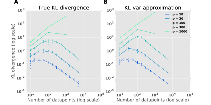
Figure 1: Evolution of the KL divergence with $n$ in a logistic regression model. A: evolution of the true KL divergence $KL\left(g_{LAP},f\right)$ with the number of datapoints $n$. Color indicates the dimension $p$ of the model. For every value of $\left(n,p\right)$, multiple simulations were performed (dots). The line corresponds to the average over these simulations. The KL divergence asymptotes as $n^{-1}$ for large values of $n$, but is also small for small values of $n$ when the posterior is almost equal to the Gaussian prior. Usual asymptotic arguments only identify the large $n$ asymptotic behavior. B: evolution of the $KL_{var}$ approximation of $KL\left(g_{LAP},f\right)$ with $n$. The approximation successfully recovers the full range of the dynamics of the KL divergence. Note that the asymptote hasn’t been reached yet for the larger values of $p$.

Throughout the range of values I explored, the KL variance proved to be a great approximation of the KL divergence (Fig.2.A). Indeed, the ratio of the KL-variance-based approximation of $KL\left(g_{LAP},f\right)$ to the truth is mostly close to $1$ and only has a maximum of $5$.

The ratio of the “LSI+KLvar” approximation to the true KL divergence is similarly close to $1$(Fig.2.B). However, the ratio is always above $1$, indicating that this approximation is always strictly bigger than the KL divergence, thus confirming the approximate upper-bound status of this approximation.

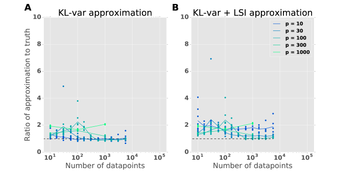
Figure 2: Quality of the KL-var and the "KL-var + LSI" approximations. A: evolution of the ratio $\frac{1}{2}KL_{var}/KL$ as a function of $n$. A ratio above $1$ indicates overestimation of the true KL divergence. Throughout the range of parameters explored, $KL_{var}$ yields a tight approximation of the KL divergence. B: same as A for the "KL-var + LSI" approximation of Cor.7. This approximation consistently upper-bounds the KL divergence in the experiment. Note that the upper-bound behavior is more pronounced for small values of $p$. This is unsurprising since the LSI term is $p$-times smaller than the $KL_{var}$ term (Cor.7).

Finally, the varELBO and Taylor-based approximations proved to be very disappointing. The varELBO was mostly uncomputable when compared to the alternatives. This is due to the fact that computing the varELBO requires computing an empirical mean over the radius $r\sim g\left(r\right)$, thus increasing the number of samples required by an order of magnitude. However, for the small values of $n,p$ for which the varELBO remained computable, it was almost equal to $KL_{var}$ (Appendix Fig.F.3.C).

Taylor-based approximations are similarly very expensive to compute since they require the manipulation of the $d^{3}$ coefficients of $\tilde{\phi}_{f}^{\left(3\right)}\left(0\right)$ and $d^{4}$ coefficients of $\tilde{\phi}_{f}^{\left(4\right)}\left(0\right)$. This proved doable for $p\in\left\{10,30,100\right\}$. However, in this range, the Taylor-based approximations were quite disappointing in comparison with the corresponding approximations based on empirical means. Indeed, most Taylor-based approximation were five to ten times bigger than the truth for small values of $n$ and only became good approximations when the large-data limit behavior dominated. This is probably due to the fact that Taylor approximations of $\tilde{\phi}_{f}\left(\boldsymbol{\theta}\right)$ are unrepresentative of its shape for small values of $n$ due to them being too local in this regime (Appendix Fig.F.3.D-G).

Overall, the KL variance and the “LSI+KLvar” approximations appear to yield great approximations of $KL\left(g_{LAP},f\right)$ in the examples considered here. Indeed, both are always in the correct order of magnitude. Furthermore, the KL-variance approximation is close to being exact in both the small $n$ and large $n$ regimes. In contrast, the varELBO approximations and the Taylor-based approximations appear to be dominated. Indeed, they are computationally trickier while yielding worse approximations.

5 Discussion

In this article, I have presented a new Bernstein-von Mises theorem which aims at being more computationally relevant than existing results. I have shown that, in a limit where a log-concave probability distribution has higher derivatives that are small compared to the second derivative, the Laplace approximation becomes exact (Th.5). This result can be used to rederive the classical BvM result that the posterior is asymptotically Gaussian for IID data (Cor.6). However, the main draw of Th.5 is the fact that it yields several computable approximations (Cor.7) of the KL divergence $KL\left(g_{LAP},f\right)$ and in particular an approximation based on the “KL variance”:

$$KL\left(g_{LAP},f\right) \approx\frac{1}{2}KL_{var}\left(g_{LAP},f\right)$$ (93)

$$\approx\frac{1}{2}\text{Var}_{\boldsymbol{\theta}\sim g_{LAP}\left(\boldsymbol{\theta}\right)}\left[\phi_{f}\left(\boldsymbol{\theta}\right)-\phi_{g}\left(\boldsymbol{\theta}\right)\right]$$ (94)

This approximation can thus be used to compute an indicator of the quality of the Laplace approximation of a given log-concave posterior.

5.1 Validating the Laplace approximation using $KL\left(g_{LAP},f\right)$

Knowledge of the KL divergence $KL\left(g_{LAP},f\right)$ can be used to validate whether, in a given problem, it is a valid approximation or not. Indeed, knowing or bounding the KL divergence can be used in two different ways to assess whether $g_{LAP}\left(\boldsymbol{\theta}\right)$ is indeed a good approximation of the target $f\left(\boldsymbol{\theta}\right)$.

First, we can use knowledge of $KL\left(g_{LAP},f\right)$ to derive whether credible intervals of $g_{LAP}$ have good coverage under $f$. Indeed, for any region $R$, the probabilities:

$$p_{g} =\mathbb{P}\left(\boldsymbol{\theta}_{g}\in R\right)$$ (95)

$$p_{f} =\mathbb{P}\left(\boldsymbol{\theta}_{f}\in R\right)$$

must be such that:

$$p_{g}\log\left(\frac{p_{g}}{p_{f}}\right)+\left(1-p_{g}\right)\log\left(\frac{1-p_{g}}{1-p_{f}}\right)\leq KL\left(g_{LAP},f\right)$$ (96)

This yields an upper and a lower bound on $p_{f}$ given the KL divergence and $p_{g}$ and can thus be used to derive regions with guaranteed coverage under $f$.

Second, knowledge of the KL divergence can be used to approximate the marginal likelihood of the data under the model in Bayesian inference which is a quantity required to perform model comparison. Given multiple Bayesian models of a dataset $\mathcal{D}=d$, a posterior distribution over the models can be constructed by computing the marginal likelihood of the data under each model:

$$f_{M_{i}}\left(\mathcal{D}=d\right)=\int f_{M_{i}}\left(\mathcal{D}=d|\boldsymbol{\theta}\right)f_{M_{i}}\left(\boldsymbol{\theta}\right)d\boldsymbol{\theta}$$ (97)

This quantity is very hard to estimate but it can be approximated using an approximation of the posterior density $g\left(\boldsymbol{\theta}\right)\approx f_{M_{i}}\left(\boldsymbol{\theta}|\mathcal{D}=d\right)$ through the Evidence Lower Bound (ELBO):

$$\log\left(f_{M_{i}}\left(\mathcal{D}=d\right)\right) \geq ELBO$$ (98)

$$\geq\mathbb{E}_{\boldsymbol{\theta}\sim g\left(\boldsymbol{\theta}\right)}\left[\log\frac{f_{M_{i}}\left(\mathcal{D}=d|\boldsymbol{\theta}\right)f_{M_{i}}\left(\boldsymbol{\theta}\right)}{g\left(\boldsymbol{\theta}\right)}\right]$$ (99)

where the error of this approximation is precisely equal to the KL divergence $KL\left(g\left(\boldsymbol{\theta}\right),f_{M_{i}}\left(\boldsymbol{\theta}|\mathcal{D}=d\right)\right)$. Control of the KL divergence can thus enable rigorous Bayesian model comparison based on the ELBO.

Theorem 5 and Cor.7 thus provide a path towards rigorous Bayesian inference based on the Laplace approximation through approximating or bounding $KL\left(g_{LAP},f\right)$ and then assessing precisely the error introduced by extrapolating inferences drawn from $g_{LAP}$ to the true posterior $f$. My experiments hint at $KL_{var}$ and the “KLvar+LSI” combination being the best approximations for this purpose since they offered respectively a tight approximation and tight upper-bound of the true KL divergence, while being straightforward to compute.

5.2 Assumptions

It is instructive to consider the assumptions I propose here in great detail, and in particular to compare them to the classical assumptions of the BvM theorem.

In classical approaches to BvM results, global control is achieved instead by assuming that the posterior concentrates around $\boldsymbol{\theta}_{0}$. My assumption of the posterior being log-concave is considerably stronger and implies consistency. This is due to log-concave distributions being strongly concentrated around their posterior distribution (Pereyra (2016)). Weakening this assumption on the posterior would thus considerably expand the applicability of Theorem 5 but this appears quite challenging since the LSI will not be applicable anymore to bound $KL\left(r_{g},r_{f}|\boldsymbol{e}\right)$.

In contrast, my assumption that the posterior has controlled third derivatives is much closer to the equivalent assumption that the log-likelihood is Locally Asymptotically Normal (LAN; Van der Vaart (2000) Ch.7). These conditions state that around $\boldsymbol{\theta}_{0}$, a quadratic approximation of the log-likelihood is asymptotically valid which ensures in turn that the Laplace approximation of the posterior is asymptotically correct. My assumption is stronger in that I assume that a third derivative exists and that it is globally bounded while LAN behavior can emerge with less regularity. For example, the likelihood of a Laplace distribution does not have a second derivative, but still leads to asymptotically Gaussian posteriors. However, extending Theorem 5 to these circumstances appears to be straightforward and I will pursue it in further work.

Finally, note that the assumption that every neighborhood of $\boldsymbol{\theta}_{0}$ has non-zero prior probability is implied by the assumption controlling the third derivatives of the prior (eq.(71)). Indeed, if the third derivative is bounded, then the prior must spread its mass over all of $\mathbb{R}^{p}$ and it is impossible for the prior not to put mass on all neighborhood of $\boldsymbol{\theta}_{0}$.

It seems to me straightforward to check whether the posterior in a given model respects the conditions outlined in here. It might be possible to directly assess whether the posterior is log-concave directly. Alternatively, it is also possible to guarantee that the posterior is log-concave by combining a log-concave prior with log-concave likelihoods (such as those of the linear logistic classification model considered in this article). Indeed, log-concavity is clearly conserved by products. Controlling the derivatives of the posterior is similarly straightforward. The easiest possibility consists in deriving an upper-bound on the third derivative of the negative log-likelihood. This upper-bound can be quite pessimistic since the precise value of $\Delta_{3}$ does not come into play in the $KL_{var}$ approximation of $KL\left(g_{LAP},f\right)$.

5.3 Scaling with dimensionality

An important aspect of modern asymptotics is the fact the dimensionality $p$ might be comparable to $n$, thus complexifying the asymptotic analysis. In this work, I have established in Theorem 5 that the KL divergence tends to $0$ at least as $\left(\Delta_{3}\right)^{2}p^{3}$ in the limit. However, I am doubtful that the exponent of $p$ is accurate here since it might instead reflect limits of the proof. While additional work is required to acquire definite understanding of the scaling $p$, the following examples are instructive.

First, I present an example that saturates the bound. Consider a target density $f\left(\boldsymbol{\theta}\right)$ such that:

$$\tilde{\phi}_{f}\left(\tilde{\boldsymbol{\theta}}\right)\approx\frac{1}{2}\left\|\tilde{\boldsymbol{\theta}}\right\|_{2}^{2}+\frac{1}{6}\Delta_{3}\text{sign}\left(\tilde{\theta}_{1}\right)\left\|\tilde{\boldsymbol{\theta}}\right\|_{2}^{3}$$ (100)

Note that this target is not continuous in $\tilde{\boldsymbol{\theta}}$ due to the discontinuity at $\tilde{\theta}_{1}=0$ so it does not quite fit the assumptions of Theorem 5 but we can still try to compute the quality of the approximation with the standard Gaussian $\tilde{g}\left(\tilde{\boldsymbol{\theta}}\right)$. Careful examination reveals that the proof of Theorem 5 would still hold for this example since I only actually use continuity in $r$ of $\tilde{\phi}_{f}\left(r\boldsymbol{e}\right)$. To understand $KL\left(g,f\right)$, first compute the ELBO approximation of $\log\left[f\left(\boldsymbol{e}\right)\right]$:

$$\log\left[f\left(\boldsymbol{e}\right)\right] \approx\mathbb{E}_{r\sim g_{LAP}\left(r\right)}\left[\tilde{\phi}_{f}\left(r\boldsymbol{e}\right)-\tilde{\phi}_{g}\left(\boldsymbol{e}\right)\right]+C$$ (101)

$$\approx\frac{1}{6}\Delta_{3}\text{sign}\left(e_{1}\right)\mathbb{E}\left(r_{g}^{3}\right)+C$$ (102)

$$\approx\frac{1}{6}\Delta_{3}\text{sign}\left(e_{1}\right)p^{3/2}+C$$ (103)

The distribution of $\boldsymbol{e}_{f}$ is thus uniform on the two half spheres $e_{1}>0$ and $e_{1}<0$. The KL divergence then scales as the variance of $\log\left[f\left(\boldsymbol{e}\right)\right]$ (Prop.1):

$$KL\left(g_{LAP},f\right)=\mathcal{O}\left(\left(\Delta_{3}\right)^{2}p^{3}\right)$$ (104)

Thus, this example is such that the limit behavior indeed is reached at the rate $\left(\Delta_{3}\right)^{2}p^{3}$ predicted by Theorem 5. However, this example is less regular than assumed by the Theorem and is not representative of the typical posterior distribution. More regular targets $\phi_{f}\left(\boldsymbol{\theta}\right)$ might have improved scaling in $p$.

In particular, modifying the assumptions on the local control of $\phi_{f}\left(\boldsymbol{\theta}\right)$ might change the exponent of $p$ in the asymptotic behavior. Indeed, if the posterior is such that $\tilde{\phi}_{f}\left(\tilde{\boldsymbol{\theta}}\right)-\tilde{\phi}_{g}\left(\tilde{\boldsymbol{\theta}}\right)$ grows at $\left\|\tilde{\boldsymbol{\theta}}\right\|_{2}^{k}$ instead of $\left\|\tilde{\boldsymbol{\theta}}\right\|_{2}^{3}$ as assumed here, we should expect at most a growth at rate $p^{k}$ because:

$$\text{Var}_{\boldsymbol{\theta}\sim g_{LAP}\left(\boldsymbol{\theta}\right)}\left[\phi_{f}\left(\boldsymbol{\theta}\right)-\phi_{g}\left(\boldsymbol{\theta}\right)\right] =\text{Var}_{\tilde{\boldsymbol{\theta}}\sim\tilde{g}_{LAP}\left(\tilde{\boldsymbol{\theta}}\right)}\left[\tilde{\phi}_{f}\left(\tilde{\boldsymbol{\theta}}\right)-\tilde{\phi}_{g}\left(\tilde{\boldsymbol{\theta}}\right)\right]$$ (105)

$$\leq\mathbb{E}_{\tilde{\boldsymbol{\theta}}\sim\tilde{g}_{LAP}\left(\tilde{\boldsymbol{\theta}}\right)}\left[\tilde{\phi}_{f}\left(\tilde{\boldsymbol{\theta}}\right)-\tilde{\phi}_{g}\left(\tilde{\boldsymbol{\theta}}\right)\right]^{2}$$ (106)

$$\leq\mathbb{E}\left(\left\|\tilde{\boldsymbol{\theta}}\right\|_{2}^{2k}\right)$$ (107)

$$\apprle p^{k}$$ (108)

More generally, structural assumptions on the target $\phi_{f}\left(\boldsymbol{\theta}\right)$ can have a heavy impact on the dimensionality scaling. For example, if the target distribution factorizes over each component: $f\left(\boldsymbol{\theta}\right)=\prod_{i=1}^{p}f\left(\theta_{i}\right)$, then the Laplace approximation also factorizes, and we have:

$$\text{Var}_{\boldsymbol{\theta}\sim g_{LAP}\left(\boldsymbol{\theta}\right)}\left[\phi_{f}\left(\boldsymbol{\theta}\right)-\phi_{g}\left(\boldsymbol{\theta}\right)\right] =\sum_{i=1}^{p}\text{Var}_{\theta_{i}\sim g_{LAP}\left(\theta_{i}\right)}\left[\phi_{f}\left(\theta_{i}\right)-\phi_{g}\left(\theta_{i}\right)\right]$$ (109)

$$\leq p\Delta_{3}\mathbb{E}\left(\theta^{6}\right)$$ (110)

The scaling with dimensionality of the main term of Theorem 5 scales only as $p$ instead of $p^{3}$. However, note that Theorem 5 would still require $\Delta_{3}p^{3/2}\rightarrow 0$ in order to guarantee that the additional error terms go to $0$. Once again, I must emphasize that this might reflect a limit of the proof and that the approximations of Cor.7 might be valid even for faster growth of $p$.

5.4 Limits

Finally, please beware that quite a bit of care must be taken when using the $KL_{var}$ approximation of the KL divergence to ensure mathematical rigor.

Indeed, this approximation requires the asymptote $\Delta_{3}p^{3/2}\rightarrow 0$ to be reached. I have established that this asymptote is reached as $n\rightarrow\infty$ in the classical IID setting (Cor.6) and I conjecture that it generally holds whenever the posterior has a Gaussian limit, but further work will be required to check this conjecture. Intuitively, the KL variance approximation should furthermore yield a good approximation of the KL divergence when $n$ is small and the prior is close to Gaussian but further theoretical work is needed to establish this rigorously.

It is furthermore critical to keep in mind the key restriction that $f$ needs to be log-concave in order for Theorem 5 to apply. Indeed, it is straightforward to design counter-examples, such as the mixture of a thin and wide Gaussian discussed in Section 3.1, for which the KL variance is arbitrarily close to $0$ while the KL divergence is arbitrarily big. Using the KL variance approximation might thus be inappropriate in the absence of an argument to ensure that most of the mass of $f$ is concentrated around its mode.

Another more trivial limit is the fact that the KL divergence $KL\left(g_{LAP},f\right)$ is infinite if the support of $f$ is not $\mathbb{R}^{p}$. Careful application of Theorem 5 would reveal this immediately since the support of $f$ being strictly smaller than $\mathbb{R}^{p}$ requires $\Delta_{3}=\infty$. The KLvar approximation of the KL divergence would also be infinite but empirical approximations of $KL_{var}\left(g_{LAP},f\right)$ might fail to recover this infinite value. It is thus necessary to check the support of $f$.

Finally, it is critical to notice that the present work only applies to the Laplace approximation of $f$. Indeed, several important modern alternatives, such as the Gaussian Variational approximation or mean-field approximations (i.e. Gaussian approximation with a Diagonal or block-Diagonal covariance; Blei et al. (2017)), are not covered by Theorem 5. Non Gaussian approximations are also not covered. While it is possible that the KL variance gives a possible measure of the quality of such approximations, additional work is required to determine this rigorously.

6 Conclusion

In this article, I have shown that, under assumptions, it is asymptotically valid to approximate the KL divergence between a posterior distribution and its Laplace approximation by using one-half of the KL variance instead. This gives a computable measure of the quality of the Laplace approximation that can then be used to measure the error induced by this approximation, and thus assessing whether the it is acceptable, or needs to be replaced by another more precise approximation of the posterior. Future work will be required to assess if this approximation of the KL divergence can be extended to other approximations and weaker assumptions.

Appendix

This appendix provides detailed proofs of every claim I make in the main text of the article and gives details of how to reproduce the empirical findings. Proofs are contained in Sections A-E. Details of the empirical study of the logistic classification model are given in Section F.

Each section deals with the proof of one result in the main text:

• Section A proves Prop.1.

• Section B proves Prop.3 and 4.

• Section C proves Th.5.

• Section D proves Cor.6.

• Section E proves Cor.7.

Since the sequence of proofs is quite involved, I have tried to maximize its readability in the following ways. Each section starts with a detailed description of the structure of the proof of the corresponding claim. The Lemmas proved in each section are almost only required inside the corresponding section. Each Lemma and Proposition of this appendix details its “parents” in the dependency structure of this proof.

Appendix A The $KL_{var}$ approximation

This section deals with the proof of Prop.1 which asserts that, under limiting assumptions, the KL variance can be used as an approximation for the KL divergence.

Recall that throughout this section, $f\left(\boldsymbol{\theta}\right)$ and $g\left(\boldsymbol{\theta}\right)$ can be any probability densities:

$$f\left(\boldsymbol{\theta}\right) =\exp\left(-\phi_{f}\left(\boldsymbol{\theta}\right)-\log\left(Z_{f}\right)\right)$$ (111)

$$g\left(\boldsymbol{\theta}\right) =\exp\left(-\phi_{g}\left(\boldsymbol{\theta}\right)-\log\left(Z_{g}\right)\right)$$ (112)

A.1 Proof structure

This proof is fairly straightforward. The following results are established in order:

• First, I establish that, for any densities $f\left(\boldsymbol{\theta}\right)$ and $g\left(\boldsymbol{\theta}\right)$, the KL divergence can be rewritten in a way that discards the log-normalizing constants (Lemma 8).

• Then, I prove that the family:

  $$h\left(\boldsymbol{\theta};\lambda\right) =g\left(\boldsymbol{\theta}\right)\left[\frac{f\left(\boldsymbol{\theta}\right)}{g\left(\boldsymbol{\theta}\right)}\right]^{\lambda}\exp\left[-C\left(\lambda\right)\right]\ \ \lambda\in\left[0,1\right]$$ (113)

  $$C\left(\lambda\right) =\log\left\{\int g\left(\boldsymbol{\theta}\right)\left[\frac{f\left(\boldsymbol{\theta}\right)}{g\left(\boldsymbol{\theta}\right)}\right]^{\lambda}d\boldsymbol{\theta}\right\}$$ (114)

  exists and is an exponential family (Lemma 9).

• Then, I establish key properties of a function $\tilde{C}\left(\lambda\right)$ that is closely related to the cumulant generating function $C\left(\lambda\right)$ (Lemma 10).

• Then, I give a bound on the cumulants of a bounded random variable (Lemma 11).

• Finally, I define the function:

  $$K\left(\lambda\right)=KL\left(g\left(\boldsymbol{\theta}\right),h\left(\boldsymbol{\theta};\lambda\right)\right)$$ (115)

  and show how to approximate it using the KL variance (Lemma 12).

These results then yield Prop.1.

A.2 Proofs

Lemma 8.

Another formula for $KL\left(g,f\right)$.

Requires: NA.

The KL divergence:

$$KL\left(g,f\right) =\mathbb{E}_{\boldsymbol{\theta}\sim g\left(\boldsymbol{\theta}\right)}\left[\log\frac{g\left(\boldsymbol{\theta}\right)}{f\left(\boldsymbol{\theta}\right)}\right]$$ (116)

$$=\mathbb{E}_{\boldsymbol{\theta}\sim g\left(\boldsymbol{\theta}\right)}\left[\phi_{f}\left(\boldsymbol{\theta}\right)+\log\left(Z_{f}\right)-\phi_{g}\left(\boldsymbol{\theta}\right)-\log\left(Z_{g}\right)\right]$$ (117)

can be rewritten with no reference to the normalizing constants:

$$KL\left(g,f\right)=\mathbb{E}_{\boldsymbol{\theta}\sim g\left(\boldsymbol{\theta}\right)}\left[\phi_{f}\left(\boldsymbol{\theta}\right)-\phi_{g}\left(\boldsymbol{\theta}\right)\right]+\log\left\{\mathbb{E}_{\boldsymbol{\theta}\sim g\left(\boldsymbol{\theta}\right)}\left[\exp\left(\phi_{g}\left(\boldsymbol{\theta}\right)-\phi_{f}\left(\boldsymbol{\theta}\right)\right)\right]\right\}$$ (118)

Proof.

This proof results from a straightforward manipulation of the expression of $KL\left(g,f\right)$.

Starting from the usual formulation for $KL\left(g,f\right)$, we first remove the normalizing constants from the expected value:

$$KL\left(g,f\right) =\mathbb{E}_{\boldsymbol{\theta}\sim g\left(\boldsymbol{\theta}\right)}\left[\phi_{f}\left(\boldsymbol{\theta}\right)+\log\left(Z_{f}\right)-\phi_{g}\left(\boldsymbol{\theta}\right)-\log\left(Z_{g}\right)\right]$$ (119)

$$=\mathbb{E}_{\boldsymbol{\theta}\sim g\left(\boldsymbol{\theta}\right)}\left[\phi_{f}\left(\boldsymbol{\theta}\right)-\phi_{g}\left(\boldsymbol{\theta}\right)\right]+\log\left(Z_{f}\right)-\log\left(Z_{g}\right)$$ (120)

$$=\mathbb{E}_{\boldsymbol{\theta}\sim g\left(\boldsymbol{\theta}\right)}\left[\phi_{f}\left(\boldsymbol{\theta}\right)-\phi_{g}\left(\boldsymbol{\theta}\right)\right]+\log\left(\frac{Z_{f}}{Z_{g}}\right)$$ (121)

Let us make explicit $Z_{f}$:

$$Z_{f}=\int\exp\left(-\phi_{f}\left(\boldsymbol{\theta}\right)\right)d\boldsymbol{\theta}$$ (122)

We can rework this expression in order to make $g\left(\boldsymbol{\theta}\right)$ appear:

$$Z_{f} =\int\frac{g\left(\boldsymbol{\theta}\right)}{g\left(\boldsymbol{\theta}\right)}\exp\left(-\phi_{f}\left(\boldsymbol{\theta}\right)\right)d\boldsymbol{\theta}$$ (123)

$$=\int g\left(\boldsymbol{\theta}\right)\exp\left(\phi_{g}\left(\boldsymbol{\theta}\right)+\log\left(Z_{g}\right)-\phi_{f}\left(\boldsymbol{\theta}\right)\right)d\boldsymbol{\theta}$$ (124)

$$=Z_{g}\int g\left(\boldsymbol{\theta}\right)\exp\left(\phi_{g}\left(\boldsymbol{\theta}\right)-\phi_{f}\left(\boldsymbol{\theta}\right)\right)d\boldsymbol{\theta}$$ (125)

$$\frac{Z_{f}}{Z_{g}} =\mathbb{E}_{\boldsymbol{\theta}\sim g\left(\boldsymbol{\theta}\right)}\left[\exp\left(\phi_{g}\left(\boldsymbol{\theta}\right)-\phi_{f}\left(\boldsymbol{\theta}\right)\right)\right]$$ (126)

Returning to eq.(121) with this final expression, we obtain the claimed result:

$$KL\left(g,f\right) =\mathbb{E}_{\boldsymbol{\theta}\sim g\left(\boldsymbol{\theta}\right)}\left[\phi_{f}\left(\boldsymbol{\theta}\right)-\phi_{g}\left(\boldsymbol{\theta}\right)\right]+\log\left(\frac{Z_{f}}{Z_{g}}\right)$$ (127)

$$=\mathbb{E}_{\boldsymbol{\theta}\sim g\left(\boldsymbol{\theta}\right)}\left[\phi_{f}\left(\boldsymbol{\theta}\right)-\phi_{g}\left(\boldsymbol{\theta}\right)\right]+\log\left\{\mathbb{E}_{\boldsymbol{\theta}\sim g\left(\boldsymbol{\theta}\right)}\left[\exp\left(\phi_{g}\left(\boldsymbol{\theta}\right)-\phi_{f}\left(\boldsymbol{\theta}\right)\right)\right]\right\}$$ (128)

which concludes this proof. ∎

Lemma 9.

The $h\left(\boldsymbol{\theta};\lambda\right)$ family.

Requires: NA.

The family of distributions:

$$h\left(\boldsymbol{\theta};\lambda\right) =g\left(\boldsymbol{\theta}\right)\left[\frac{f\left(\boldsymbol{\theta}\right)}{g\left(\boldsymbol{\theta}\right)}\right]^{\lambda}\exp\left[-C\left(\lambda\right)\right]\ \ \lambda\in\left[0,1\right]$$ (129)

$$=g\left(\boldsymbol{\theta}\right)\exp\left(\lambda\left[\phi_{g}\left(\boldsymbol{\theta}\right)-\phi_{f}\left(\boldsymbol{\theta}\right)\right]-\tilde{C}\left(\lambda\right)\right)$$ (130)

$$C\left(\lambda\right) =\log\left\{\int g\left(\boldsymbol{\theta}\right)\left[\frac{f\left(\boldsymbol{\theta}\right)}{g\left(\boldsymbol{\theta}\right)}\right]^{\lambda}d\boldsymbol{\theta}\right\}$$ (131)

$$\tilde{C}\left(\lambda\right) =\log\left\{\mathbb{E}_{\boldsymbol{\theta}\sim g\left(\boldsymbol{\theta}\right)}\left[\exp\left(\lambda\left[\phi_{g}\left(\boldsymbol{\theta}\right)-\phi_{f}\left(\boldsymbol{\theta}\right)\right]\right)\right]\right\}$$ (132)

exists and is an exponential family.

Proof.

This Lemma contains multiple statements that we will check in order.

First, let us prove that the family does exist. This requires proving that the function $C\left(\lambda\right)$ takes finite values over the range $\lambda\in]0,1[$. This follows from the Holder inequality with $p=\left(1-\lambda\right)^{-1}$ and $q=\lambda^{-1}$ such that $p^{-1}+q^{-1}=1$:

$$\int g\left(\boldsymbol{\theta}\right)\left[\frac{f\left(\boldsymbol{\theta}\right)}{g\left(\boldsymbol{\theta}\right)}\right]^{\lambda}d\boldsymbol{\theta} =\int\left[g\left(\boldsymbol{\theta}\right)\right]^{1-\lambda}\left[f\left(\boldsymbol{\theta}\right)\right]^{\lambda}d\boldsymbol{\theta}$$ (133)

$$\leq\left\{\int\left[g\left(\boldsymbol{\theta}\right)\right]^{p\left(1-\lambda\right)}d\boldsymbol{\theta}\right\}^{p^{-1}}\left\{\int\left[f\left(\boldsymbol{\theta}\right)\right]^{q\lambda}d\boldsymbol{\theta}\right\}^{q^{-1}}$$ (134)

$$\leq\left\{\int g\left(\boldsymbol{\theta}\right)d\boldsymbol{\theta}\right\}^{1-\lambda}\left\{\int f\left(\boldsymbol{\theta}\right)d\boldsymbol{\theta}\right\}^{\lambda}$$ (135)

$$\leq 1$$ (136)

Then, we have that, for all $\lambda\in\left[0,1\right]$, $h\left(\boldsymbol{\theta};\lambda\right)$ is a positive function which integrates to $1$. It is thus indeed a density. The family thus exists.

In order to see that it is indeed an exponential family, just rewrite the density:

$$h\left(\boldsymbol{\theta};\lambda\right) =g\left(\boldsymbol{\theta}\right)\left[\frac{f\left(\boldsymbol{\theta}\right)}{g\left(\boldsymbol{\theta}\right)}\right]^{\lambda}\exp\left[-C\left(\lambda\right)\right]$$ (137)

$$=g\left(\boldsymbol{\theta}\right)\exp\left(\lambda\left[\phi_{g}\left(\boldsymbol{\theta}\right)-\phi_{f}\left(\boldsymbol{\theta}\right)+\log\left(\frac{Z_{g}}{Z_{f}}\right)\right]-C\left(\lambda\right)\right)$$ (138)

This is indeed an exponential family. It has base density $g\left(\boldsymbol{\theta}\right)$, a single natural parameter $\lambda$, associated sufficient statistic $\left[\phi_{g}\left(\boldsymbol{\theta}\right)-\phi_{f}\left(\boldsymbol{\theta}\right)+\log\left(\frac{Z_{g}}{Z_{f}}\right)\right]$ and normalizing constant (or cumulant generating function) $C\left(\lambda\right)$.

We can also rewrite the exponential family as:

$$h\left(\boldsymbol{\theta};\lambda\right) =g\left(\boldsymbol{\theta}\right)\exp\left(\lambda\left[\phi_{g}\left(\boldsymbol{\theta}\right)-\phi_{f}\left(\boldsymbol{\theta}\right)+\log\left(\frac{Z_{g}}{Z_{f}}\right)\right]-C\left(\lambda\right)\right)$$ (139)

$$=g\left(\boldsymbol{\theta}\right)\exp\left(\lambda\left[\phi_{g}\left(\boldsymbol{\theta}\right)-\phi_{f}\left(\boldsymbol{\theta}\right)\right]-\lambda\left[\log\left(\frac{Z_{g}}{Z_{f}}\right)\right]-C\left(\lambda\right)\right)$$ (140)

$$=g\left(\boldsymbol{\theta}\right)\exp\left(\lambda\left[\phi_{g}\left(\boldsymbol{\theta}\right)-\phi_{f}\left(\boldsymbol{\theta}\right)\right]-\tilde{C}\left(\lambda\right)\right)$$ (141)

where:

$$\tilde{C}\left(\lambda\right) =\log\left\{\int g\left(\boldsymbol{\theta}\right)\exp\left(\lambda\left[\phi_{g}\left(\boldsymbol{\theta}\right)-\phi_{f}\left(\boldsymbol{\theta}\right)\right]\right)d\boldsymbol{\theta}\right\}$$ (142)

$$=\log\left\{\mathbb{E}_{\boldsymbol{\theta}\sim g\left(\boldsymbol{\theta}\right)}\left[\exp\left(\lambda\left[\phi_{g}\left(\boldsymbol{\theta}\right)-\phi_{f}\left(\boldsymbol{\theta}\right)\right]\right)\right]\right\}$$ (143)

This concludes the proof. ∎

Lemma 10.

Properties of $\tilde{C}\left(\lambda\right)$.

Requires: Lemma 9.

The Cumulant Generating Function:

$$\tilde{C}\left(\lambda\right)=\log\left\{\mathbb{E}_{\boldsymbol{\theta}\sim g\left(\boldsymbol{\theta}\right)}\left[\exp\left(\lambda\left[\phi_{g}\left(\boldsymbol{\theta}\right)-\phi_{f}\left(\boldsymbol{\theta}\right)\right]\right)\right]\right\}$$ (144)

is convex.

Its derivatives are the cumulants of the statistic $\phi_{g}\left(\boldsymbol{\theta}\right)-\phi_{f}\left(\boldsymbol{\theta}\right)$ for $\boldsymbol{\theta}\sim h\left(\boldsymbol{\theta};\lambda\right)$. In particular:

$$\tilde{C}^{{}^{\prime}}\left(\lambda\right) =k_{1}\left(\lambda\right)=\mathbb{E}_{\boldsymbol{\theta}\sim h\left(\boldsymbol{\theta};\lambda\right)}\left[\phi_{g}\left(\boldsymbol{\theta}\right)-\phi_{f}\left(\boldsymbol{\theta}\right)\right]$$ (145)

$$\tilde{C}^{{}^{\prime\prime}}\left(\lambda\right) =k_{2}\left(\lambda\right)=\text{Var}_{\boldsymbol{\theta}\sim h\left(\boldsymbol{\theta};\lambda\right)}\left[\phi_{g}\left(\boldsymbol{\theta}\right)-\phi_{f}\left(\boldsymbol{\theta}\right)\right]$$ (146)

$$\tilde{C}^{\left(3\right)}\left(\lambda\right) =k_{3}\left(\lambda\right)=\mathbb{E}_{\boldsymbol{\theta}\sim h\left(\boldsymbol{\theta};\lambda\right)}\left[\left\{\phi_{g}\left(\boldsymbol{\theta}\right)-\phi_{f}\left(\boldsymbol{\theta}\right)-k_{1}\left(\lambda\right)\right\}^{3}\right]$$ (147)

Proof.

This Lemma just corresponds to standard properties of exponential families and their CGF.

$\tilde{C}\left(\lambda\right)$ is defined as:

$$\tilde{C}\left(\lambda\right)=\log\left\{\mathbb{E}_{\boldsymbol{\theta}\sim g\left(\boldsymbol{\theta}\right)}\left[\exp\left(\lambda\left[\phi_{g}\left(\boldsymbol{\theta}\right)-\phi_{f}\left(\boldsymbol{\theta}\right)\right]\right)\right]\right\}$$ (148)

which we can rewrite as:

$$\exp\left[\tilde{C}\left(\lambda\right)\right] =\mathbb{E}_{\boldsymbol{\theta}\sim g\left(\boldsymbol{\theta}\right)}\left[\exp\left(\lambda\left[\phi_{g}\left(\boldsymbol{\theta}\right)-\phi_{f}\left(\boldsymbol{\theta}\right)\right]\right)\right]$$ (149)

$$=\int g\left(\boldsymbol{\theta}\right)\exp\left(\lambda\left[\phi_{g}\left(\boldsymbol{\theta}\right)-\phi_{f}\left(\boldsymbol{\theta}\right)\right]\right)d\boldsymbol{\theta}$$ (150)

$$=\int\exp\left(-\phi_{g}\left(\boldsymbol{\theta}\right)-\log\left(Z_{g}\right)-\lambda\left[\phi_{g}\left(\boldsymbol{\theta}\right)-\phi_{f}\left(\boldsymbol{\theta}\right)\right]\right)d\boldsymbol{\theta}$$ (151)

$$=\frac{1}{Z_{g}}\int\exp\left(-\left(1-\lambda\right)\phi_{g}\left(\boldsymbol{\theta}\right)-\lambda\phi_{f}\left(\boldsymbol{\theta}\right)\right)d\boldsymbol{\theta}$$ (152)

Let us now prove the convexity of $\tilde{C}\left(\lambda\right)$. Let $\lambda_{1}<\lambda_{2}<\lambda_{3}$. Without loss of generality, we can assume that $\lambda_{1}=0$ and $\lambda_{3}=1$ and $\lambda=\lambda_{2}$ which simply corresponds to considering new functions $g\left(\boldsymbol{\theta}\right)=h\left(\boldsymbol{\theta};\lambda_{1}\right)$ and $f\left(\boldsymbol{\theta};\lambda_{3}\right)$. Now apply Holder inequality to $\tilde{C}\left(\lambda\right)$ with $p=\left(1-\lambda\right)$ and $q=\lambda^{-1}$:

$$\int\exp\left(-\left(1-\lambda\right)\phi_{g}\left(\boldsymbol{\theta}\right)-\lambda\phi_{f}\left(\boldsymbol{\theta}\right)\right)d\boldsymbol{\theta}\leq\left[\int\exp\left(-\phi_{g}\left(\boldsymbol{\theta}\right)\right)d\boldsymbol{\theta}\right]^{1-\lambda}\left[\int\exp\left(-\phi_{f}\left(\boldsymbol{\theta}\right)\right)d\boldsymbol{\theta}\right]^{\lambda}$$ (153)

We thus have:

$$\tilde{C}\left(\lambda\right) =\log\left[\frac{1}{Z_{g}}\int\exp\left(-\left(1-\lambda\right)\phi_{g}\left(\boldsymbol{\theta}\right)-\lambda\phi_{f}\left(\boldsymbol{\theta}\right)\right)d\boldsymbol{\theta}\right]$$ (154)

$$\leq-\left(1-\lambda+\lambda\right)\log\left(Z_{g}\right)+\left(1-\lambda\right)\log\left[\int\exp\left(-\phi_{g}\left(\boldsymbol{\theta}\right)\right)d\boldsymbol{\theta}\right]+\lambda\log\left[\int\exp\left(-\phi_{f}\left(\boldsymbol{\theta}\right)\right)d\boldsymbol{\theta}\right]$$ (155)

$$\leq\left(1-\lambda\right)\tilde{C}\left(0\right)+\lambda\tilde{C}\left(1\right)$$ (156)

which establishes the convexity of $\tilde{C}\left(\lambda\right)$.

The derivatives of a CGF are (like the name indicates) the cumulants of the associated sufficient statistic. The first derivative of $\tilde{C}\left(\lambda\right)$ is thus the mean of $\phi_{g}\left(\boldsymbol{\theta}\right)-\phi_{f}\left(\boldsymbol{\theta}\right)$. Its second derivative is similarly the covariance. The third derivative is slightly more tricky to state since it is the third cumulant which is defined, for a variable $X$, as:

$$k_{3}\left(X\right)=\mathbb{E}\left[\left\{X-\mathbb{E}\left(X\right)\right\}^{3}\right]$$ (157)

These cumulants are computed under the density $h\left(\boldsymbol{\theta};\lambda\right)$.

For example, the calculation of the first derivative yields:

$$\tilde{C}^{{}^{\prime}}\left(\lambda\right) =\frac{\partial}{\partial\lambda}\log\left\{\mathbb{E}_{\boldsymbol{\theta}\sim g\left(\boldsymbol{\theta}\right)}\left[\exp\left(\lambda\left[\phi_{g}\left(\boldsymbol{\theta}\right)-\phi_{f}\left(\boldsymbol{\theta}\right)\right]\right)\right]\right\}$$ (158)

$$=\frac{\int g\left(\boldsymbol{\theta}\right)\frac{\partial}{\partial\lambda}\exp\left(\lambda\left[\phi_{g}\left(\boldsymbol{\theta}\right)-\phi_{f}\left(\boldsymbol{\theta}\right)\right]\right)d\boldsymbol{\theta}}{\int g\left(\boldsymbol{\theta}\right)\exp\left(\lambda\left[\phi_{g}\left(\boldsymbol{\theta}\right)-\phi_{f}\left(\boldsymbol{\theta}\right)\right]\right)d\boldsymbol{\theta}}$$ (159)

$$=\frac{\int g\left(\boldsymbol{\theta}\right)\left[\phi_{g}\left(\boldsymbol{\theta}\right)-\phi_{f}\left(\boldsymbol{\theta}\right)\right]\exp\left(\lambda\left[\phi_{g}\left(\boldsymbol{\theta}\right)-\phi_{f}\left(\boldsymbol{\theta}\right)\right]\right)d\boldsymbol{\theta}}{\int g\left(\boldsymbol{\theta}\right)\exp\left(\lambda\left[\phi_{g}\left(\boldsymbol{\theta}\right)-\phi_{f}\left(\boldsymbol{\theta}\right)\right]\right)d\boldsymbol{\theta}}$$ (160)

$$=\int g\left(\boldsymbol{\theta}\right)\left[\phi_{g}\left(\boldsymbol{\theta}\right)-\phi_{f}\left(\boldsymbol{\theta}\right)\right]\exp\left(\lambda\left[\phi_{g}\left(\boldsymbol{\theta}\right)-\phi_{f}\left(\boldsymbol{\theta}\right)\right]-\tilde{C}\left(\lambda\right)\right)d\boldsymbol{\theta}$$ (161)

$$=\mathbb{E}_{\boldsymbol{\theta}\sim h\left(\boldsymbol{\theta};\lambda\right)}\left[\phi_{g}\left(\boldsymbol{\theta}\right)-\phi_{f}\left(\boldsymbol{\theta}\right)\right]$$ (162)

This concludes the proof. ∎

Lemma 11.

Approximation of $KL\left(g\left(\boldsymbol{\theta}\right),h\left(\boldsymbol{\theta};\lambda\right)\right)$.

Requires: Lemmas 8-10.

The KL divergence between $g\left(\boldsymbol{\theta}\right)$ and $h\left(\boldsymbol{\theta};\lambda\right)$:

$$KL\left(g\left(\boldsymbol{\theta}\right),h\left(\boldsymbol{\theta};\lambda\right)\right) =K\left(\lambda\right)$$ (163)

$$=\lambda\mathbb{E}_{\boldsymbol{\theta}\sim g\left(\boldsymbol{\theta}\right)}\left[\phi_{f}\left(\boldsymbol{\theta}\right)-\phi_{g}\left(\boldsymbol{\theta}\right)\right]+\log\left\{\mathbb{E}_{\boldsymbol{\theta}\sim g\left(\boldsymbol{\theta}\right)}\left[\exp\left(\lambda\left[\phi_{g}\left(\boldsymbol{\theta}\right)-\phi_{f}\left(\boldsymbol{\theta}\right)\right]\right)\right]\right\}$$ (164)

$$=\lambda\mathbb{E}_{\boldsymbol{\theta}\sim g\left(\boldsymbol{\theta}\right)}\left[\phi_{f}\left(\boldsymbol{\theta}\right)-\phi_{g}\left(\boldsymbol{\theta}\right)\right]+\tilde{C}\left(\lambda\right)$$ (165)

has a Taylor approximation with integral remainder:

$$K\left(\lambda\right) =0+0+\frac{\lambda^{2}}{2}\text{Var}_{\boldsymbol{\theta}\sim g\left(\boldsymbol{\theta}\right)}\left[\phi_{g}\left(\boldsymbol{\theta}\right)-\phi_{f}\left(\boldsymbol{\theta}\right)\right]+\int_{0}^{\lambda}\frac{1}{2}l^{2}k_{3}\left(l\right)dl$$ (166)

$$k_{3}\left(\lambda\right) =\mathbb{E}_{\boldsymbol{\theta}\sim h\left(\boldsymbol{\theta};\lambda\right)}\left[\left\{\phi_{g}\left(\boldsymbol{\theta}\right)-\phi_{f}\left(\boldsymbol{\theta}\right)-k_{1}\left(\lambda\right)\right\}^{3}\right]$$ (167)

$$k_{1}\left(\lambda\right) =\mathbb{E}_{\boldsymbol{\theta}\sim h\left(\boldsymbol{\theta};\lambda\right)}\left[\phi_{g}\left(\boldsymbol{\theta}\right)-\phi_{f}\left(\boldsymbol{\theta}\right)\right]$$ (168)

Proof.

This proof follows from Lemmas 8 and 9, which yield that $K\left(\lambda\right)$ is indeed a correct formula for $KL\left(g\left(\boldsymbol{\theta}\right),h\left(\boldsymbol{\theta};\lambda\right)\right)$, and then a straightforward manipulation of $K\left(\lambda\right)$.

First, let us check that the formula for $K\left(\lambda\right)$ is indeed correct. Lemma 9 gives us the log-density of $h\left(\boldsymbol{\theta};\lambda\right)$:

$$h\left(\boldsymbol{\theta};\lambda\right) =g\left(\boldsymbol{\theta}\right)\left[\frac{f\left(\boldsymbol{\theta}\right)}{g\left(\boldsymbol{\theta}\right)}\right]^{\lambda}\exp\left(-C\left(\boldsymbol{\theta}\right)\right)$$ (169)

$$=\exp\left(-\phi_{g}\left(\boldsymbol{\theta}\right)+\lambda\left[\phi_{g}\left(\boldsymbol{\theta}\right)-\phi_{f}\left(\boldsymbol{\theta}\right)\right]-\log\left(Z_{g}\right)-\tilde{C}\left(\boldsymbol{\theta}\right)\right)$$ (170)

Lemma 8 asserts that we can ignore the normalizing constant terms $-\log\left(Z_{g}\right)-\tilde{C}\left(\boldsymbol{\theta}\right)$. One unnormalized negative log-density for $h$ is:

$$\phi_{h}\left(\boldsymbol{\theta}\right)=\phi_{g}\left(\boldsymbol{\theta}\right)-\lambda\left[\phi_{g}\left(\boldsymbol{\theta}\right)-\phi_{f}\left(\boldsymbol{\theta}\right)\right]$$ (171)

and Lemma 8 then gives us the KL divergence as:

$$K\left(\lambda\right) =\mathbb{E}_{\boldsymbol{\theta}\sim g\left(\boldsymbol{\theta}\right)}\left[\phi_{h}\left(\boldsymbol{\theta}\right)-\phi_{g}\left(\boldsymbol{\theta}\right)\right]+\log\left\{\mathbb{E}_{\boldsymbol{\theta}\sim g\left(\boldsymbol{\theta}\right)}\left[\exp\left(\phi_{g}\left(\boldsymbol{\theta}\right)-\phi_{h}\left(\boldsymbol{\theta}\right)\right)\right]\right\}$$ (172)

$$=\mathbb{E}_{\boldsymbol{\theta}\sim g\left(\boldsymbol{\theta}\right)}\left[-\lambda\left[\phi_{g}\left(\boldsymbol{\theta}\right)-\phi_{f}\left(\boldsymbol{\theta}\right)\right]\right]+\log\left\{\mathbb{E}_{\boldsymbol{\theta}\sim g\left(\boldsymbol{\theta}\right)}\left[\exp\left(\lambda\left[\phi_{g}\left(\boldsymbol{\theta}\right)-\phi_{f}\left(\boldsymbol{\theta}\right)\right]\right)\right]\right\}$$ (173)

$$=\lambda\mathbb{E}_{\boldsymbol{\theta}\sim g\left(\boldsymbol{\theta}\right)}\left[\phi_{f}\left(\boldsymbol{\theta}\right)-\phi_{g}\left(\boldsymbol{\theta}\right)\right]+\log\left\{\mathbb{E}_{\boldsymbol{\theta}\sim g\left(\boldsymbol{\theta}\right)}\left[\exp\left(\lambda\left[\phi_{g}\left(\boldsymbol{\theta}\right)-\phi_{f}\left(\boldsymbol{\theta}\right)\right]\right)\right]\right\}$$ (174)

In the formula for $K\left(\lambda\right)$, we recognize $\tilde{C}\left(\lambda\right)$ in the second term:

$$K\left(\lambda\right) =\lambda\mathbb{E}_{\boldsymbol{\theta}\sim g\left(\boldsymbol{\theta}\right)}\left[\phi_{f}\left(\boldsymbol{\theta}\right)-\phi_{g}\left(\boldsymbol{\theta}\right)\right]+\log\left\{\mathbb{E}_{\boldsymbol{\theta}\sim g\left(\boldsymbol{\theta}\right)}\left[\exp\left(\lambda\left[\phi_{g}\left(\boldsymbol{\theta}\right)-\phi_{f}\left(\boldsymbol{\theta}\right)\right]\right)\right]\right\}$$ (175)

$$=\lambda\mathbb{E}_{\boldsymbol{\theta}\sim g\left(\boldsymbol{\theta}\right)}\left[\phi_{f}\left(\boldsymbol{\theta}\right)-\phi_{g}\left(\boldsymbol{\theta}\right)\right]+\tilde{C}\left(\lambda\right)$$ (176)

The derivatives of $K\left(\lambda\right)$ at $\lambda=0$ are then straightforward to compute:

$$K\left(0\right) =0+\tilde{C}\left(0\right)$$ (177)

$$=\log\left\{\mathbb{E}_{\boldsymbol{\theta}\sim g\left(\boldsymbol{\theta}\right)}\left[\exp\left(0\left[\phi_{g}\left(\boldsymbol{\theta}\right)-\phi_{f}\left(\boldsymbol{\theta}\right)\right]\right)\right]\right\}$$ (178)

$$=\log\left\{\mathbb{E}_{\boldsymbol{\theta}\sim g\left(\boldsymbol{\theta}\right)}\left[\exp\left(0\right)\right]\right\}$$ (179)

$$=\log\left\{\mathbb{E}_{\boldsymbol{\theta}\sim g\left(\boldsymbol{\theta}\right)}\left[1\right]\right\}$$ (180)

$$=0$$ (181)

$$K^{{}^{\prime}}\left(0\right) =\mathbb{E}_{\boldsymbol{\theta}\sim g\left(\boldsymbol{\theta}\right)}\left[\phi_{f}\left(\boldsymbol{\theta}\right)-\phi_{g}\left(\boldsymbol{\theta}\right)\right]+\mathbb{E}_{\boldsymbol{\theta}\sim g\left(\boldsymbol{\theta}\right)}\left[\phi_{g}\left(\boldsymbol{\theta}\right)-\phi_{f}\left(\boldsymbol{\theta}\right)\right]$$ (182)

$$=0$$ (183)

$$K^{{}^{\prime\prime}}\left(0\right) =0+\text{Var}_{\boldsymbol{\theta}\sim g\left(\boldsymbol{\theta}\right)}\left[\phi_{g}\left(\boldsymbol{\theta}\right)-\phi_{f}\left(\boldsymbol{\theta}\right)\right]$$ (184)

and for $d\geq 2$, the derivatives of $K\left(\lambda\right)$ coincide with that of $\tilde{C}\left(\lambda\right)$:

$$K^{\left(d\right)}\left(\lambda\right) =\tilde{C}^{\left(d\right)}\left(\lambda\right)$$ (185)

$$=k_{d}\left(\lambda\right)$$ (186)

A Taylor expansion of $K\left(\lambda\right)$ to third order with integral remainder then yields:

$$K\left(\lambda\right) =K\left(0\right)+\lambda K^{{}^{\prime}}\left(0\right)+\frac{\lambda^{2}}{2}K^{{}^{\prime\prime}}\left(0\right)+\int_{0}^{\lambda}\frac{1}{2}l^{2}K^{\left(3\right)}\left(\lambda\right)dl$$ (187)

$$=0+0+\frac{\lambda^{2}}{2}\text{Var}_{\boldsymbol{\theta}\sim g\left(\boldsymbol{\theta}\right)}\left[\phi_{g}\left(\boldsymbol{\theta}\right)-\phi_{f}\left(\boldsymbol{\theta}\right)\right]+\int_{0}^{\lambda}\frac{1}{2}l^{2}k_{3}\left(l\right)dl$$ (188)

which concludes the proof. ∎

Lemma 12.

Bound on the cumulants.

Requires: NA.

If $X$ is a bounded random variable:

$$\left|X\right|\leq M$$ (189)

Then its absolute cumulants for $k\in\left\{1,2,3\right\}$ are bounded:

$$\mathbb{E}\left(\left|X-\mathbb{E}\left(X\right)\right|^{k}\right)\leq M^{k}$$ (190)

Proof.

The proof proceeds in two steps. First, we prove that the worst case is a Bernoulli random variable taking values $\pm M$ with probabilities $p$ and $\left(1-p\right)$. Then, we derive the worst value of $p$ which gives the claimed bound.

The first step of the proof using an elegant “coupling” construction: for any bounded variable $X$, we will construct a correlated variable $Y$ which has the same mean but which is more extreme. $Y$ then has higher cumulants than $X$.

We construct $Y$ conditional on $X$. Given $X=x$, we would like the conditional mean of $Y$ to be equal to $x$. The following probabilities achieve this goal:

$$p =\frac{\left(x+M\right)}{2M}$$ (191)

$$\mathbb{P}\left(Y=+M|X=x\right) =p$$ (192)

$$\mathbb{P}\left(Y=-M|X=x\right) =1-p$$ (193)

If $x=M$, then we always have $Y=x$. As $x$ decreases, $Y$ becomes more variable and is maximally variable at $x=0$ where $p=0.5$. As $x$ decreases further, $Y$ becomes less variable until $x=-M$ where we always have $Y=x=-M$.

Note that $\mathbb{E}\left(Y|X\right)=X$ and we thus have that both variables have the same mean:

$$\mathbb{E}\left(Y\right)=\mathbb{E}\left(X\right)=e$$ (194)

Now, for $k\geq 1$, consider the function:

$$a_{k}\left(t\right)=\left|t-e\right|^{k}$$ (195)

This function is convex and its expected value is the $k^{th}$ absolute cumulant.

It is straightforward to compare the expected value of $a_{k}\left(X\right)$ and $a_{k}\left(Y\right)$. Indeed, compute the expected value of $a_{k}\left(Y\right)$ by conditioning on $X$ as an intermediate step:

$$\mathbb{E}\left[a_{k}\left(Y\right)\right]=\mathbb{E}\left[\mathbb{E}\left\{a_{k}\left(Y\right)|X\right\}\right]$$ (196)

Applying Jensen’s inequality to the convex function $a_{k}\left(t\right)$ for $X=x$:

$$\mathbb{E}\left\{a_{k}\left(Y\right)|X=x\right\} \geq a_{k}\left(\mathbb{E}\left\{Y|X=x\right\}\right)$$ (197)

$$\geq a_{k}\left(x\right)$$ (198)

We thus finally have:

$$\mathbb{E}\left[a_{k}\left(Y\right)\right] =\mathbb{E}\left[\mathbb{E}\left\{a_{k}\left(Y\right)|X\right\}\right]$$ (199)

$$\geq\mathbb{E}\left[a_{k}\left(X\right)\right]$$ (200)

and we have proved that $Y$ has a higher cumulant than $X$. Since $Y$ only takes the values $\pm M$, it is thus marginally a Bernoulli random variable. Bernoulli random variables thus have the biggest cumulants among bounded random variables.

It is now straightforward to compute the cumulant of a Bernoulli random variable with probability $p$:

$$\mathbb{E}\left(Y\right) =Mp-\left(1-p\right)M$$ (201)

$$=M\left(2p-1\right)$$ (202)

$$\mathbb{E}\left(\left|Y-\mathbb{E}\left(Y\right)\right|^{k}\right) =p\left|M-M\left(2p-1\right)\right|^{k}+\left(1-p\right)\left|-M-M\left(2p-1\right)\right|^{k}$$ (203)

$$=pM^{k}\left|2-2p\right|^{k}+\left(1-p\right)M^{k}\left|2p\right|^{k}$$ (204)

$$=2^{k}M^{k}\left[p\left(1-p\right)^{k}+\left(1-p\right)p^{k}\right]$$ (205)

$$=2^{k}M^{k}p\left(1-p\right)\left[\left(1-p\right)^{k-1}+p^{k-1}\right]$$ (206)

and we only need to optimize for $p$.

Consider the polynomial in $p$:

$$A\left(p\right)=p\left(1-p\right)\left[\left(1-p\right)^{k-1}+p^{k-1}\right]$$ (207)

The gradient of $A\left(p\right)$ is:

$$A^{{}^{\prime}}\left(p\right) =\left(1-p\right)\left[\left(1-p\right)^{k-1}+p^{k-1}\right]-p\left[\left(1-p\right)^{k-1}+p^{k-1}\right]$$

$$\ \ \ \ +p\left(1-p\right)\left[-\left(k-1\right)\left(1-p\right)^{k-2}+\left(k-1\right)p^{k-2}\right]$$ (208)

$$=\left(1-2p\right)\left[\left(1-p\right)^{k-1}+p^{k-1}\right]+\left(k-1\right)p\left(1-p\right)\left[-\left(1-p\right)^{k-2}+p^{k-2}\right]$$ (209)

For $k=1$ or $k=2$, we have that $A^{{}^{\prime}}\left(p\right)$ is monotone with a unique zero at $p=0.5$.

$$\text{If }k=1\ \ A^{{}^{\prime}}\left(p\right) =\left(1-2p\right)\left(2\right)+0$$ (210)

$$=2\left(1-2p\right)$$ (211)

$$\text{If }k=2\ \ A^{{}^{\prime}}\left(p\right) =\left(1-2p\right)\left(1-p+p\right)+p\left(1-p\right)\left(-1+1\right)$$ (212)

$$=\left(1-2p\right)$$ (213)

For $k=3$:

$$A^{{}^{\prime}}\left(p\right) =\left(1-2p\right)\left[\left(1-p\right)^{2}+p^{2}\right]+2p\left(1-p\right)\left[-\left(1-p\right)+p\right]$$ (214)

$$=\left(1-2p\right)\left[\left(1-p\right)^{2}+p^{2}\right]+2p\left(1-p\right)\left[2p-1\right]$$ (215)

$$=\left(1-2p\right)\left[\left(1-p\right)^{2}+p^{2}-2p\left(1-p\right)\right]$$ (216)

$$=\left(1-2p\right)\left[\left(1-p-p\right)^{2}\right]$$ (217)

$$=\left(1-2p\right)^{3}$$ (218)

Once again $A^{\prime}\left(p\right)$ is monotone and has a unique zero at $p=0.5$.

The maximum of $\mathbb{E}\left(\left|Y-\mathbb{E}\left(Y\right)\right|^{k}\right)$ for $k\in\left\{1,2,3\right\}$ is thus:

$$\mathbb{E}\left(\left|Y-\mathbb{E}\left(Y\right)\right|^{k}\right) \leq 2^{k}M^{k}\frac{1}{2}\frac{1}{2}\left(\left(\frac{1}{2}\right)^{k-1}+\left(\frac{1}{2}\right)^{k-1}\right)$$ (219)

$$\leq 2^{k}M^{k}\frac{2}{2^{k+1}}$$ (220)

$$\leq M^{k}$$ (221)

which gives the claimed bound.

∎

At this point, we are now ready to give the proof of Prop.1.

Proof.

The statement of Prop.1 combines elements from the various Lemmas of this Appendix Section.

Lemma 9 asserts that $h\left(\boldsymbol{\theta};\lambda\right)$ is indeed an exponential family.

Then, Lemma 11 (in the special case $\lambda=1$) asserts that the KL divergence $KL\left(g,f\right)$ can be approximated using a Taylor expansion.

Finally, we get to the case for which $\left|\phi_{f}\left(\boldsymbol{\theta}\right)-\phi_{g}\left(\boldsymbol{\theta}\right)\right|\leq M$. Lemma 12 gives a bound on the absolute cumulants of $\phi_{f}\left(\boldsymbol{\theta}\right)-\phi_{g}\left(\boldsymbol{\theta}\right)$: they must be lower than $M^{3}$.

The Taylor expansion with integral remainder of $KL\left(g,f\right)$ can then be further simplified by bounding the integral remainder:

$$\left|\int_{0}^{1}\frac{1}{2}l^{2}k_{3}\left(l\right)dl\right| \leq\int_{0}^{1}\frac{1}{2}l^{2}\left|k_{3}\left(l\right)\right|dl$$ (222)

$$\leq\int_{0}^{1}\frac{1}{2}l^{2}M^{3}dl$$ (223)

$$\leq\frac{M^{3}}{6}$$ (224)

which concludes the proof. ∎

Appendix B The LSI-based approximations

This section deals with the proof of Prop.3 and 4 which give upper-bounds on the forward and backward KL divergences based on the Log-Sobolev Inequality (LSI).

Recall that throughout this section, $g\left(\boldsymbol{\theta}\right)$ is not restricted to being the Laplace approximation of $f\left(\boldsymbol{\theta}\right)$ and is not necessarily restricted to being Gaussian.

B.1 Proof structure

The proof of both propositions is fairly straightforward:

• First, I establish a variant of the classical LSI result which is invariant to affine reparameterizations of the space. This is exactly Prop.3

• Finally, I prove Prop.4, as a straightforward corollary from Prop.3.

B.2 Proofs

First, recall the classical statement of the LSI. Or, more precisely, of the fact that strongly log-concave distributions obey the LSI.

Theorem 13.

LSI (Bakry and Émery [1985], Otto and Villani [2000]).

If $f\left(\boldsymbol{\theta}\right)$ is a $\lambda$-strongly log-concave density, i.e.

$$\forall\boldsymbol{\theta}\ H\phi_{f}\left(\boldsymbol{\theta}\right)\geq\lambda I_{p}$$ (225)

then, for any $g\left(\boldsymbol{\theta}\right)$, the reverse KL divergence is bounded:

$$KL\left(g,f\right)\leq\frac{1}{2\lambda}\mathbb{E}_{\boldsymbol{\theta}\sim g\left(\boldsymbol{\theta}\right)}\left[\left\|\nabla\phi_{f}\left(\boldsymbol{\theta}\right)-\nabla\phi_{g}\left(\boldsymbol{\theta}\right)\right\|_{2}^{2}\right]$$ (226)

A trivial limit of this Theorem is that it is not invariant to affine reparameterizations of the parameter space. Indeed, these modify the gradients and $\lambda$ simultaneously in a way that does not lead to the terms canceling.

However, this limit is trivial since it can be solved by making sure that the inequality $\forall\boldsymbol{\theta}\ H\phi_{f}\left(\boldsymbol{\theta}\right)\geq\lambda I_{p}$ is tight in all eigenvalues at once. This yields Prop.3.

Proposition 14.

Main text Prop.3: an affine equivariant LSI.

Requires: Th.13.

If $f\left(\boldsymbol{\theta}\right)$ is strongly log-concave so that there exists a strictly positive matrix $H_{min}$ such that:

$$\forall\boldsymbol{\theta}\ H\phi_{f}\left(\boldsymbol{\theta}\right)\geq H_{min}$$ (227)

then, for any approximation $g\left(\boldsymbol{\theta}\right)$, the reverse KL divergence is bounded:

$$KL\left(g,f\right)\leq\frac{1}{2}\mathbb{E}_{\boldsymbol{\theta}\sim g\left(\boldsymbol{\theta}\right)}\left[\left\{\nabla\phi_{f}\left(\boldsymbol{\theta}\right)-\nabla\phi_{g}\left(\boldsymbol{\theta}\right)\right\}^{T}\left(H_{min}\right)^{-1}\left\{\nabla\phi_{f}\left(\boldsymbol{\theta}\right)-\nabla\phi_{g}\left(\boldsymbol{\theta}\right)\right\}\right]$$ (228)

Proof.

Consider a matrix square-root of $\left[H_{min}\right]^{-1}$: $AA^{T}=\left[H_{min}\right]^{-1}$. Then, consider the change of variable:

$$\mathring{\boldsymbol{\theta}}=A\boldsymbol{\theta}$$ (229)

Log-gradients and log-Hessians in $\mathring{\boldsymbol{\theta}}$-space are:

$$\nabla_{\mathring{\boldsymbol{\theta}}}\mathring{\phi}_{f}\left(\mathring{\boldsymbol{\theta}}\right) =A\nabla_{\boldsymbol{\theta}}\phi_{f}\left(A\boldsymbol{\theta}\right)$$ (230)

$$H_{\mathring{\boldsymbol{\theta}}}\mathring{\phi}_{f}\left(\mathring{\boldsymbol{\theta}}\right) =A\ H\phi_{f}\left(A\boldsymbol{\theta}\right)\ A^{T}$$ (231)

In $\mathring{\boldsymbol{\theta}}$-space, the log-Hessian density is still lower-bounded:

$$\forall\mathring{\boldsymbol{\theta}}\ H_{\mathring{\boldsymbol{\theta}}}\mathring{\phi}_{f}\left(\mathring{\boldsymbol{\theta}}\right) \geq AH_{min}A^{T}$$ (232)

$$\geq I_{p}$$ (233)

We can thus apply Thm.13 with $\lambda=1$, yielding:

$$KL\left(\mathring{\boldsymbol{\theta}}_{g},\mathring{\boldsymbol{\theta}}_{f}\right) \leq\frac{1}{2}\mathbb{E}_{\mathring{\boldsymbol{\theta}}\sim g\left(\mathring{\boldsymbol{\theta}}\right)}\left[\left\|\nabla_{\mathring{\boldsymbol{\theta}}}\mathring{\phi}_{f}\left(\mathring{\boldsymbol{\theta}}\right)-\nabla_{\mathring{\boldsymbol{\theta}}}\mathring{\phi}_{g}\left(\mathring{\boldsymbol{\theta}}\right)\right\|_{2}^{2}\right]$$ (234)

$$\leq\frac{1}{2}\mathbb{E}_{\boldsymbol{\theta}\sim g\left(\boldsymbol{\theta}\right)}\left[\left\|A\nabla_{\boldsymbol{\theta}}\phi_{f}\left(A\boldsymbol{\theta}\right)-A\nabla_{\boldsymbol{\theta}}\phi_{g}\left(A\boldsymbol{\theta}\right)\right\|_{2}^{2}\right]$$ (235)

$$\leq\frac{1}{2}\mathbb{E}_{\boldsymbol{\theta}\sim g\left(\boldsymbol{\theta}\right)}\left[\left\|A\left\{\nabla_{\boldsymbol{\theta}}\phi_{f}\left(A\boldsymbol{\theta}\right)-\nabla_{\boldsymbol{\theta}}\phi_{g}\left(A\boldsymbol{\theta}\right)\right\}\right\|_{2}^{2}\right]$$ (236)

$$\leq\frac{1}{2}\mathbb{E}_{\boldsymbol{\theta}\sim g\left(\boldsymbol{\theta}\right)}\left[\left\{\nabla\phi_{f}\left(\boldsymbol{\theta}\right)-\nabla\phi_{g}\left(\boldsymbol{\theta}\right)\right\}^{T}AA^{T}\left\{\nabla\phi_{f}\left(\boldsymbol{\theta}\right)-\nabla\phi_{g}\left(\boldsymbol{\theta}\right)\right\}\right]$$ (237)

$$\leq\frac{1}{2}\mathbb{E}_{\boldsymbol{\theta}\sim g\left(\boldsymbol{\theta}\right)}\left[\left\{\nabla\phi_{f}\left(\boldsymbol{\theta}\right)-\nabla\phi_{g}\left(\boldsymbol{\theta}\right)\right\}^{T}\left(H_{min}\right)^{-1}\left\{\nabla\phi_{f}\left(\boldsymbol{\theta}\right)-\nabla\phi_{g}\left(\boldsymbol{\theta}\right)\right\}\right]$$ (238)

Finally, observe that the KL divergence is invariant to bijective changes of variable:

$$KL\left(g,f\right) =KL\left(\mathring{\boldsymbol{\theta}}_{g},\mathring{\boldsymbol{\theta}}_{f}\right)$$ (239)

$$\leq\frac{1}{2}\mathbb{E}_{\boldsymbol{\theta}\sim g\left(\boldsymbol{\theta}\right)}\left[\left\{\nabla\phi_{f}\left(\boldsymbol{\theta}\right)-\nabla\phi_{g}\left(\boldsymbol{\theta}\right)\right\}^{T}\left(H_{min}\right)^{-1}\left\{\nabla\phi_{f}\left(\boldsymbol{\theta}\right)-\nabla\phi_{g}\left(\boldsymbol{\theta}\right)\right\}\right]$$ (240)

which concludes the proof. ∎

Proposition 15.

Main text Prop.4: a straightforward corollary.

Requires: Appendix Prop.14 (Main text Prop.3).

If $g\left(\boldsymbol{\theta}\right)$ is a Gaussian with covariance $\Sigma$, then for any $f\left(\boldsymbol{\theta}\right)$ the forward KL divergence is bounded:

$$KL\left(f,g\right)\leq\frac{1}{2}\mathbb{E}_{\boldsymbol{\theta}\sim f\left(\boldsymbol{\theta}\right)}\left[\left\{\nabla\phi_{f}\left(\boldsymbol{\theta}\right)-\nabla\phi_{g}\left(\boldsymbol{\theta}\right)\right\}^{T}\Sigma\left\{\nabla\phi_{f}\left(\boldsymbol{\theta}\right)-\nabla\phi_{g}\left(\boldsymbol{\theta}\right)\right\}\right]$$ (241)

Proof.

This proof is a straightforward corollary of Appendix Prop.14 (Main text Prop.3). It is derived by inverting the role of $g$ and $f$.

Indeed, if $g\left(\boldsymbol{\theta}\right)$ is a Gaussian with covariance $\Sigma$, then:

$$\phi_{g} =\frac{1}{2}\left(\boldsymbol{\theta}-\boldsymbol{\mu}\right)^{T}\Sigma^{-1}\left(\boldsymbol{\theta}-\boldsymbol{\mu}\right)$$ (242)

$$H\phi_{g} =\Sigma^{-1}$$ (243)

and we can thus apply Appendix Prop.14 with $H_{min}=\Sigma^{-1}$ yielding, with no assumption on $f\left(\boldsymbol{\theta}\right)$:

$$KL\left(g,f\right) \leq\frac{1}{2}\mathbb{E}_{\boldsymbol{\theta}\sim f\left(\boldsymbol{\theta}\right)}\left[\left\{\nabla\phi_{f}\left(\boldsymbol{\theta}\right)-\nabla\phi_{g}\left(\boldsymbol{\theta}\right)\right\}^{T}\left[\Sigma^{-1}\right]^{-1}\left\{\nabla\phi_{f}\left(\boldsymbol{\theta}\right)-\nabla\phi_{g}\left(\boldsymbol{\theta}\right)\right\}\right]$$ (244)

$$\leq\frac{1}{2}\mathbb{E}_{\boldsymbol{\theta}\sim f\left(\boldsymbol{\theta}\right)}\left[\left\{\nabla\phi_{f}\left(\boldsymbol{\theta}\right)-\nabla\phi_{g}\left(\boldsymbol{\theta}\right)\right\}^{T}\Sigma\left\{\nabla\phi_{f}\left(\boldsymbol{\theta}\right)-\nabla\phi_{g}\left(\boldsymbol{\theta}\right)\right\}\right]$$ (245)

which concludes the proof. ∎

Appendix C General deterministic Bound

This section deals with the proof of Th.5, establishing the convergence of $KL\left(g,f\right)$ to $0$ in the limit $\Delta_{3}p^{3/2}\rightarrow 0$, as well as several approximations of this quantity.

Throughout this section, we will simplify notation by using $g\left(\boldsymbol{\theta}\right)$ for the Laplace approximation of $f\left(\boldsymbol{\theta}\right)$ (dropping out the index from $g_{LAP}\left(\boldsymbol{\theta}\right)$). We also assume that $f\left(\boldsymbol{\theta}\right)$ is strictly log-concave. All results stated from this point onward are restricted to this case.

We recall the notation:

$$f\left(\boldsymbol{\theta}\right) =\exp\left(-\phi_{f}\left(\boldsymbol{\theta}\right)-\log\left(Z_{f}\right)\right)$$ (246)

$$H\phi_{f}\left(\boldsymbol{\theta}\right) >0_{p}$$ (247)

$$g\left(\boldsymbol{\theta}\right) =\exp\left(-\phi_{g}\left(\boldsymbol{\theta}\right)-\log\left(Z_{g}\right)\right)$$ (248)

$$=\exp\left(-\frac{1}{2}\left(\boldsymbol{\theta}-\boldsymbol{\mu}\right)^{T}\Sigma^{-1}\left(\boldsymbol{\theta}-\boldsymbol{\mu}\right)-\log\left(Z_{g}\right)\right)$$ (249)

$$\boldsymbol{\mu} =\text{argmin}_{\boldsymbol{\theta}}\left[\phi_{f}\left(\boldsymbol{\theta}\right)\right]$$ (250)

$$\Sigma^{-1} =H\phi_{f}\left(\boldsymbol{\mu}\right)$$ (251)

C.1 Proof structure

The proof of this result is very involved.

1. First, I tackle aspects of the proof relating to the variables $r,\boldsymbol{e}$ and $c,\boldsymbol{e}$. I show the following results:

   1. I establish that $KL\left(g,f\right)$ can be decomposed into the contributions of the variables $r$ and $\boldsymbol{e}$ (Lemma 16).

   2. I give the distribution of $\boldsymbol{e},r$ under $g$ (Lemma 17).

   3. I give the distribution of $c=\left(r\right)^{1/3}$ under $g$ (Lemma 18).

   4. I give the moments of $r$ under $g$ (Lemma 19).

   5. I give (Lemma 20):

      • The conditional distribution of $r$ under $f$.

      • The conditional distribution of $c$ under $f$.

      • The marginal distribution of $\boldsymbol{e}$ under $f$.

      • An approximation to the marginal distribution of $\boldsymbol{e}$ under $f$.

2. Then, I tackle the $KL\left(r_{g},r_{f}|\boldsymbol{e}\right)$ term and derive the following results:

   1. I prove that $f\left(c\right)$ is strongly log-concave (Lemma 22).

   2. I give a lower-bound of the log-curvature of $f\left(c\right)$ (Lemmas 23 and 24).

   3. I give the asymptotic scaling of the lower-bound (Lemma 26).

   4. I give an approximation of $KL\left(r_{g},r_{f}|\boldsymbol{e}\right)$ based on Appendix Prop.14 (Main text Prop.3) (Prop.27).

3. Then, I tackle the $KL\left(\boldsymbol{e}_{g},\boldsymbol{e}_{f}\right)$ term. I further show the following results:

   1. I give an approximation of $\log\left[f\left(\boldsymbol{e}\right)\right]$ (Lemma 28).

   2. I give an approximation of $KL\left(\boldsymbol{e}_{g},\boldsymbol{e}_{f}\right)$ based on Appendix Prop.14 (Main text Prop.3) (Prop.29).

4. Finally, I relate the bound on $KL\left(\boldsymbol{e}_{g},\boldsymbol{e}_{f}\right)$ to the KL variance (Lemma 30).

Theorem. 5 is finally derived as a combination of all the results proved in this section.

C.2 Proofs: properties of the change of variable

Lemma 16.

Decomposition of $KL\left(g,f\right)$.

Requires: NA.

The KL divergence can be decomposed as:

$$KL\left(g,f\right)=KL\left(\boldsymbol{e}_{g},\boldsymbol{e}_{f}\right)+\mathbb{E}_{\boldsymbol{e}\sim g\left(\boldsymbol{e}\right)}\left[KL\left(r_{g},r_{f}|\boldsymbol{e}\right)\right]$$ (252)

Proof.

This proof consists of a simple manipulation of the normal expression for the KL divergence.

We simply make appear the variables $r,\boldsymbol{e}$:

$$KL\left(g,f\right) =\mathbb{E}_{\boldsymbol{\theta}\sim g\left(\boldsymbol{\theta}\right)}\left[\log\frac{f\left(\boldsymbol{\theta}\right)}{g\left(\boldsymbol{\theta}\right)}\right]$$ (253)

$$=\mathbb{E}_{r,\boldsymbol{e}\sim g\left(r,\boldsymbol{e}\right)}\left[\log\frac{f\left(r,\boldsymbol{e}\right)}{g\left(r,\boldsymbol{e}\right)}\right]$$ (254)

and then use the conditional probability formula:

$$f\left(r,\boldsymbol{e}\right) =f\left(\boldsymbol{e}\right)f\left(r|\boldsymbol{e}\right)$$ (255)

$$g\left(r,\boldsymbol{e}\right) =g\left(\boldsymbol{e}\right)g\left(r|\boldsymbol{e}\right)$$ (256)

yielding:

$$KL\left(g,f\right) =\mathbb{E}_{r,\boldsymbol{e}\sim g\left(r,\boldsymbol{e}\right)}\left[\log\frac{f\left(\boldsymbol{e}\right)f\left(r|\boldsymbol{e}\right)}{g\left(\boldsymbol{e}\right)g\left(r|\boldsymbol{e}\right)}\right]$$ (257)

$$=\mathbb{E}_{r,\boldsymbol{e}\sim g\left(r,\boldsymbol{e}\right)}\left[\log\frac{f\left(\boldsymbol{e}\right)}{g\left(\boldsymbol{e}\right)}+\log\frac{f\left(r|\boldsymbol{e}\right)}{g\left(r|\boldsymbol{e}\right)}\right]$$ (258)

$$=\mathbb{E}_{\boldsymbol{e}\sim g\left(\boldsymbol{e}\right)}\left[\log\frac{f\left(\boldsymbol{e}\right)}{g\left(\boldsymbol{e}\right)}\right]+\mathbb{E}_{r,\boldsymbol{e}\sim g\left(r,\boldsymbol{e}\right)}\left[\log\frac{f\left(r|\boldsymbol{e}\right)}{g\left(r|\boldsymbol{e}\right)}\right]$$ (259)

$$=KL\left(\boldsymbol{e}_{g},\boldsymbol{e}_{f}\right)+\mathbb{E}_{\boldsymbol{e}\sim g\left(\boldsymbol{e}\right)}\left\{\mathbb{E}_{r\sim g\left(r|\boldsymbol{e}\right)}\left[\log\frac{f\left(r|\boldsymbol{e}\right)}{g\left(r|\boldsymbol{e}\right)}\right]\right\}$$ (260)

$$=KL\left(\boldsymbol{e}_{g},\boldsymbol{e}_{f}\right)+\mathbb{E}_{\boldsymbol{e}\sim g\left(\boldsymbol{e}\right)}\left[KL\left(r_{g},r_{f}|\boldsymbol{e}\right)\right]$$ (261)

which concludes the proof. ∎

Lemma 17.

Distribution of $r_{g},\boldsymbol{e}_{g}$.

Requires: NA.

The random variables $r_{g},\boldsymbol{e}_{g}$ are independent. $\boldsymbol{e}_{g}$ has a uniform distribution over the unit sphere $S^{p-1}$ while $r_{g}$ has a $\chi_{p}$ distribution.

Proof.

This proof is a standard of statistics and probability theory.

Start from $\tilde{\boldsymbol{\theta}}_{g}$ which is a standard Gaussian random variable:

$$g\left(\tilde{\boldsymbol{\theta}}\right)\propto\exp\left(-\frac{1}{2}\left\|\tilde{\boldsymbol{\theta}}\right\|_{2}^{2}\right)$$ (262)

The volume of the element $drd\boldsymbol{e}$ scales as $r^{p-1}$ because it lives on the surface of a $p$-dimensional sphere of radius $r$. The standard change of variable formula then yields:

$$g\left(r,\boldsymbol{e}\right) \propto r^{p-1}\exp\left(-\frac{1}{2}\left\|r\boldsymbol{e}\right\|_{2}^{2}\right)$$ (263)

$$\propto r^{p-1}\exp\left(-\frac{1}{2}r^{2}\right)$$ (264)

which proves the well-known result:

• $\boldsymbol{e}_{g}$ is a uniform random variable over its support: the unit sphere $S^{p-1}$.

• $r_{g}$ is a $\chi$ (“chi”) random variable with $p$ degrees of freedom.

• They are independent.

and concludes the proof. ∎

Lemma 18.

Distribution of $c_{g}$.

Requires: Lemma 17.

Variable $c_{g}=\left(r_{g}\right)^{1/3}$ follows a $\chi_{p}^{1/3}$ (“chi-one-third”) distribution:

$$g\left(c\right)\propto c^{3p-1}\exp\left(-\frac{c^{6}}{2}\right)$$ (265)

Proof.

This follows from Lemma 17 through another standard change of variable:

$$g\left(c\right) \propto c^{3\left(p-1\right)}\exp\left(-\frac{c^{6}}{2}\right)\frac{dr}{dc}$$ (266)

$$\propto c^{3p-3}\exp\left(-\frac{c^{6}}{2}\right)\left(3c^{2}\right)$$ (267)

$$\propto c^{3p-1}\exp\left(-\frac{c^{6}}{2}\right)$$ (268)

which concludes the proof. ∎

Lemma 19.

Moments of $r_{g}$.

Requires: Lemma 17.

The $0$-centered moments of $r_{g}$ are:

$$\mathbb{E}\left(r_{g}^{k}\right) =2^{k/2}\frac{\Gamma\left(\frac{p+k}{2}\right)}{\Gamma\left(\frac{p}{2}\right)}$$ (269)

For fixed $k$, as $p\rightarrow\infty$, the moments of $r_{g}$ scale asymptotically as:

$$\mathbb{E}\left(r_{g}^{k}\right)=p^{k/2}+\mathcal{O}\left(p^{k/2-1}\right)$$ (270)

i.e. the ratio $r_{g}/p^{1/2}$ converges in $L_{k}$ to the constant $1$.

Proof.

The following derivation of the moments of $r_{g}$ is standard.

The normalization constant of the $\chi_{p}$ distribution is:

$$\int r^{p-1}\exp\left(-\frac{r^{2}}{2}\right)=2^{p/2-1}\Gamma\left(\frac{p}{2}\right)$$ (271)

Thus, we have the expected value of $r^{k}$ as:

$$\mathbb{E}\left[\left(r_{g}\right)^{k}\right] =\frac{\int r^{k}r^{p-1}\exp\left(-\frac{r^{2}}{2}\right)}{\int r^{p-1}\exp\left(-\frac{r^{2}}{2}\right)}$$ (272)

$$=\frac{2^{\left(p+k\right)/2-1}\Gamma\left(\frac{p+k}{2}\right)}{2^{p/2-1}\Gamma\left(\frac{p}{2}\right)}$$ (273)

$$=2^{k/2}\frac{\Gamma\left(\frac{p+k}{2}\right)}{\Gamma\left(\frac{p}{2}\right)}$$ (274)

∎

In order to approximate these moments in the limit $p\rightarrow\infty$ while $k$ remains fixed, we can consider the following approximation of the ratio of the Gamma function (see Mortici [2010] and additional references therein): for all $s\in\left[0,1\right]$

$$n^{1-s}\leq\frac{\Gamma\left(n+1\right)}{\Gamma\left(n+s\right)}\leq\left(n+1\right)^{1-s}$$ (275)

yielding:

$$\frac{\Gamma\left(n+1\right)}{\Gamma\left(n+s\right)} =n^{1-s}+\mathcal{O}\left(n^{1-s-1}\right)$$ (276)

$$=n^{1-s}+\mathcal{O}\left(n^{-s}\right)$$ (277)

in the limit $n\rightarrow\infty$.

Noting $\left\lfloor k/2\right\rfloor$ to be the highest integer smaller than $k/2$, we then further use the recurrence relationship of the Gamma function:

$$\frac{\Gamma\left[\left(p+k\right)/2\right]}{\Gamma\left[p/2\right]} =\frac{\Gamma\left[p/2+\left\lfloor k/2\right\rfloor\right]}{\Gamma\left[p/2+\left\lfloor k/2\right\rfloor\right]}\frac{\Gamma\left[p/2+k/2\right]}{\Gamma\left[p/2\right]}$$ (278)

$$=\frac{\Gamma\left[p/2+k/2\right]}{\Gamma\left[p/2+\left\lfloor k/2\right\rfloor\right]}\frac{\Gamma\left[p/2+\left\lfloor k/2\right\rfloor\right]}{\Gamma\left[p/2\right]}$$ (279)

$$=\frac{\Gamma\left[p/2+k/2\right]}{\Gamma\left[p/2+\left\lfloor k/2\right\rfloor\right]}\prod_{i=1}^{\left\lfloor k/2\right\rfloor}\frac{\left(p+i\right)}{2}$$ (280)

where the product scales asymptotically as:

$$\prod_{i=1}^{\left\lfloor k/2\right\rfloor}\frac{\left(p+i\right)}{2}=\frac{1}{2^{\left\lfloor k/2\right\rfloor}}p^{\left\lfloor k/2\right\rfloor}+\mathcal{O}\left(p^{\left\lfloor k/2\right\rfloor-1}\right)$$ (281)

while the ratio scales as:

$$\frac{\Gamma\left[p/2+k/2\right]}{\Gamma\left[p/2+\left\lfloor k/2\right\rfloor\right]}=\left(\frac{p}{2}\right)^{k/2-\left\lfloor k/2\right\rfloor}+\mathcal{O}\left(p^{k/2-\left\lfloor k/2\right\rfloor-1}\right)$$ (282)

Combining both asymptotic scalings sums the exponents, yielding:

$$\frac{\Gamma\left[\left(p+k\right)/2\right]}{\Gamma\left[p/2\right]}=\left(\frac{p}{2}\right)^{k/2}+\mathcal{O}\left(p^{k/2-1}\right)$$ (283)

which yields the asymptotic scaling of the moments:

$$\mathbb{E}\left(r_{g}^{k}\right) =2^{k/2}\frac{\Gamma\left(\frac{p+k}{2}\right)}{\Gamma\left(\frac{p}{2}\right)}$$ (284)

$$=p^{k/2}+\mathcal{O}\left(p^{k/2-1}\right)$$ (285)

which concludes the proof.

Lemma 20.

Distribution of $r_{f}|\boldsymbol{e}$, $c_{f}|\boldsymbol{e}$ and $\boldsymbol{e}_{f}$.

Requires: NA.

The conditional distribution of $r_{f}|\boldsymbol{e}$ is:

$$f\left(r|\boldsymbol{e}\right)\propto r^{p-1}\exp\left(-\tilde{\phi}_{f}\left(r\boldsymbol{e}\right)\right)$$ (286)

The conditional distribution of $c_{f}|\boldsymbol{e}$ is:

$$f\left(c|\boldsymbol{e}\right)\propto c^{3p-1}\exp\left(-\tilde{\phi}_{f}\left(c^{3}\boldsymbol{e}\right)\right)$$ (287)

The marginal distribution of $\boldsymbol{e}_{f}$ is:

$$f\left(\boldsymbol{e}\right)\propto\int r^{p-1}\exp\left(-\tilde{\phi}_{f}\left(r\boldsymbol{e}\right)\right)dr$$ (288)

where the proportionality sign hides a term that does not depend on $\boldsymbol{e}$. The marginal distribution of $\boldsymbol{e}_{f}$ can be approximated using the ELBO as:

$$\left|\log\left[f\left(\boldsymbol{e}\right)\right]-ELBO\left(\boldsymbol{e}\right)\right| \leq KL\left(r_{g},r_{f}|\boldsymbol{e}\right)$$ (289)

$$ELBO\left(\boldsymbol{e}\right) =\mathbb{E}_{r\sim g\left(r\right)}\left\{\log\left[\frac{f\left(r,\boldsymbol{e}\right)}{g\left(r\right)}\right]\right\}$$ (290)

$$=-\mathbb{E}_{r\sim g\left(r\right)}\left[\tilde{\phi}_{f}\left(r\boldsymbol{e}\right)-\frac{1}{2}r^{2}\right]+C$$ (291)

where $C$ is a constant that does not depend on $\boldsymbol{e}$.

Proof.

Like Lemma 17 and 18, the first two claims follow from a standard change of variable:

$$f\left(\tilde{\boldsymbol{\theta}}\right) \propto\exp\left(-\tilde{\phi}_{f}\left(\tilde{\boldsymbol{\theta}}\right)\right)$$ (292)

$$f\left(r,\boldsymbol{e}\right) \propto r^{p-1}\exp\left(-\tilde{\phi}_{f}\left(r\boldsymbol{e}\right)\right)$$ (293)

thus yielding:

$$f\left(r|\boldsymbol{e}\right) =\frac{f\left(r,\boldsymbol{e}\right)}{f\left(\boldsymbol{e}\right)}$$ (294)

$$\propto r^{p-1}\exp\left(-\tilde{\phi}_{f}\left(r\boldsymbol{e}\right)\right)$$ (295)

Similarly:

$$f\left(c|\boldsymbol{e}\right) \propto c^{3\left(p-1\right)}\exp\left(-\tilde{\phi}_{f}\left(c^{3}\boldsymbol{e}\right)\right)\frac{dr}{dc}$$ (296)

$$\propto c^{3\left(p-1\right)}\exp\left(-\tilde{\phi}_{f}\left(c^{3}\boldsymbol{e}\right)\right)\left(3c^{2}\right)$$ (297)

$$\propto c^{3p-1}\exp\left(-\tilde{\phi}_{f}\left(c^{3}\boldsymbol{e}\right)\right)$$ (298)

$f\left(\boldsymbol{e}\right)$ is the integral of $f\left(r,\boldsymbol{e}\right)$:

$$f\left(\boldsymbol{e}\right) =\int f\left(r,\boldsymbol{e}\right)dr$$ (299)

Combining with eq.(293), we obtain:

$$f\left(\boldsymbol{e}\right)=\frac{\int r^{p-1}\exp\left(-\tilde{\phi}_{f}\left(r\boldsymbol{e}\right)\right)dr}{\int d\boldsymbol{e}\left[\int r^{p-1}\exp\left(-\tilde{\phi}_{f}\left(r\boldsymbol{e}\right)\right)dr\right]}$$ (300)

Finally, the Evidence Lower Bound (ELBO; Blei et al. [2017]) is a well-known lower-bound on the log-integral of a density:

$$\log\left[f\left(\boldsymbol{e}\right)\right] =\log\left[\int f\left(r,\boldsymbol{e}\right)dr\right]$$ (301)

$$=\log\left[\int g\left(r\right)\frac{f\left(r,\boldsymbol{e}\right)}{g\left(r\right)}dr\right]$$ (302)

$$=\log\left[\mathbb{E}_{r\sim g\left(r\right)}\left\{\frac{f\left(r,\boldsymbol{e}\right)}{g\left(r\right)}\right\}\right]$$ (303)

$$\geq\mathbb{E}_{r\sim g\left(r\right)}\left\{\log\left[\frac{f\left(r,\boldsymbol{e}\right)}{g\left(r\right)}\right]\right\}$$ (304)

$$\geq ELBO\left(\boldsymbol{e}\right)$$ (305)

where we have used Jensen’s inequality on the concave function $t\rightarrow\log\left(t\right)$. Strictly speaking, the ELBO of $\log\left[f\left(\boldsymbol{e}\right)\right]$ is this exact expression: $\mathbb{E}_{r\sim g\left(r\right)}\left\{\log\left[\frac{f\left(r,\boldsymbol{e}\right)}{g\left(r\right)}\right]\right\}$ and the error is precisely equal to $KL\left(r_{g},r_{f}|\boldsymbol{e}\right)$.

We can rework the ELBO slightly to remove terms that are constants in $\boldsymbol{e}$:

$$\log\left[\frac{f\left(r,\boldsymbol{e}\right)}{g\left(r\right)}\right] =\log\left[\frac{r^{p-1}\exp\left(-\tilde{\phi}_{f}\left(r\boldsymbol{e}\right)\right)}{\int r^{p-1}\exp\left(-\tilde{\phi}_{f}\left(r\boldsymbol{e}\right)\right)drd\boldsymbol{e}}\frac{\int r^{p-1}\exp\left(-\frac{1}{2}r^{2}\right)drd\boldsymbol{e}}{r^{p-1}\exp\left(-\frac{1}{2}r^{2}\right)}\right]$$ (306)

$$=\log\left[\frac{r^{p-1}\exp\left(-\tilde{\phi}_{f}\left(r\boldsymbol{e}\right)\right)}{r^{p-1}\exp\left(-\frac{1}{2}r^{2}\right)}\frac{\int r^{p-1}\exp\left(-\frac{1}{2}r^{2}\right)drd\boldsymbol{e}}{\int r^{p-1}\exp\left(-\tilde{\phi}_{f}\left(r\boldsymbol{e}\right)\right)drd\boldsymbol{e}}\right]$$ (307)

$$=\log\left[\exp\left(\frac{1}{2}r^{2}-\tilde{\phi}_{f}\left(r\boldsymbol{e}\right)\right)\right]+C$$ (308)

$$=\frac{1}{2}r^{2}-\tilde{\phi}_{f}\left(r\boldsymbol{e}\right)+C$$ (309)

$$=-\left\{\tilde{\phi}_{f}\left(r\boldsymbol{e}\right)-\frac{1}{2}r^{2}\right\}+C$$ (310)

$$\mathbb{E}_{r\sim g\left(r\right)}\left\{\log\left[\frac{f\left(r,\boldsymbol{e}\right)}{g\left(r\right)}\right]\right\} =-\mathbb{E}_{r\sim g\left(r\right)}\left\{\tilde{\phi}_{f}\left(r\boldsymbol{e}\right)-\frac{1}{2}r^{2}\right\}+C$$ (311)

which yields the claimed result. Note that the $\frac{1}{2}r^{2}$ term could be dropped out too, but it corresponds to the Taylor expansion of $\tilde{\phi}_{f}\left(r\boldsymbol{e}\right)$ to second order. It thus makes sense to keep this term.

Let us finally check that the gap is indeed the KL divergence:

$$\mathbb{E}_{r\sim g\left(r\right)}\left\{\log\left[\frac{f\left(r,\boldsymbol{e}\right)}{g\left(r\right)}\right]\right\} =\mathbb{E}_{r\sim g\left(r\right)}\left\{\log\left[\frac{f\left(r|\boldsymbol{e}\right)f\left(\boldsymbol{e}\right)}{g\left(r\right)}\right]\right\}$$ (312)

$$=\mathbb{E}_{r\sim g\left(r\right)}\left\{\log\left[\frac{f\left(r|\boldsymbol{e}\right)}{g\left(r\right)}\right]\right\}+\log\left[f\left(\boldsymbol{e}\right)\right]$$ (313)

$$\log\left[f\left(\boldsymbol{e}\right)\right]-\mathbb{E}_{r\sim g\left(r\right)}\left\{\log\left[\frac{f\left(r,\boldsymbol{e}\right)}{g\left(r\right)}\right]\right\} =-\mathbb{E}_{r\sim g\left(r\right)}\left\{\log\left[\frac{f\left(r|\boldsymbol{e}\right)}{g\left(r\right)}\right]\right\}$$ (314)

$$=\mathbb{E}_{r\sim g\left(r\right)}\left\{\log\left[\frac{g\left(r\right)}{f\left(r|\boldsymbol{e}\right)}\right]\right\}$$ (315)

$$=KL\left(r_{g},r_{f}|\boldsymbol{e}\right)$$ (316)

which concludes the proof. ∎

C.3 Proofs: $KL\left(r_{g},r_{f}|\boldsymbol{e}\right)$ term.

For this section, we introduce two additional notations:

• Let $\varphi_{\boldsymbol{e}}\left(r\right)$ be the value of $\tilde{\phi}_{f}$ along direction $\boldsymbol{e}$:

  $$\varphi_{\boldsymbol{e}}\left(r\right) =\tilde{\phi}_{f}\left(r\boldsymbol{e}\right)$$ (317)

  $$=\phi_{f}\left(\boldsymbol{\mu}+r\Sigma_{g}^{1/2}\boldsymbol{e}\right)$$ (318)

• Let $\psi_{f}\left(c|\boldsymbol{e}\right)$ denote the (unnormalized) negative log-density of $f\left(c|\boldsymbol{e}\right)$:

  $$\psi_{f}\left(c|\boldsymbol{e}\right) =-\log\left[f\left(c|\boldsymbol{e}\right)\right]+C$$ (319)

  $$=-\left(3p-1\right)\log\left(c\right)+\tilde{\phi}_{f}\left(c^{3}\boldsymbol{e}\right)$$ (320)

  $$=-\left(3p-1\right)\log\left(c\right)+\varphi_{\boldsymbol{e}}\left(c^{3}\right)$$ (321)

  Similarly, let $\psi_{g}\left(c\right)$ be the negative log-density of $g\left(c\right)$:

  $$\psi_{g}\left(c\right)=-\left(3p-1\right)\log\left(c\right)+\frac{1}{2}c^{6}$$ (322)

  where we have used Lemmas 18 and 20.

Lemma 21.

Basic properties of $\varphi_{\boldsymbol{e}}\left(r\right)$.

Requires: Lemma 20.

$\varphi_{\boldsymbol{e}}\left(r\right)$ is a convex function. Its higher derivatives are controlled:

$$\left|\varphi_{\boldsymbol{e}}^{\left(3\right)}\left(r\right)\right|\leq\Delta_{3}$$

For $r\leq r_{0}=\left(\Delta_{3}\right)^{-1}$, $\varphi_{\boldsymbol{e}}\left(r\right)$ and its derivatives are bounded through a Taylor expansion:

$$\varphi_{\boldsymbol{e}}\left(r\right) \geq\frac{r^{2}}{2}-\frac{\Delta_{3}}{6}r^{3}$$ (323)

$$\varphi_{\boldsymbol{e}}^{{}^{\prime}}\left(r\right) \geq r-\frac{\Delta_{3}}{2}r^{2}$$ (324)

$$\varphi_{\boldsymbol{e}}^{{}^{\prime\prime}}\left(r\right) \geq 1-\Delta_{3}r$$ (325)

For $r\geq r_{0}=\left(\Delta_{3}\right)^{-1}$, $\varphi_{\boldsymbol{e}}\left(r\right)$ and its derivatives are bounded instead through the convexity of $\varphi_{\boldsymbol{e}}\left(r\right)$:

$$\varphi_{\boldsymbol{e}}\left(r\right) \geq\frac{1}{3}\frac{1}{\left(\Delta_{3}\right)^{2}}+\frac{1}{2\Delta_{3}}\left(r-\frac{1}{\Delta_{3}}\right)$$ (326)

$$\varphi_{\boldsymbol{e}}^{{}^{\prime}}\left(r\right) \geq\frac{1}{2\Delta_{3}}$$ (327)

$$\varphi_{\boldsymbol{e}}^{{}^{\prime\prime}}\left(r\right) \geq 0$$ (328)

Let $\varphi_{\text{min}}\left(r\right)$ be the function corresponding to the lower-bounds.

Proof.

This Lemma is proved through several straightforward manipulations of the expression for $\varphi_{\boldsymbol{e}}\left(r\right)$.

$\varphi_{\boldsymbol{e}}\left(r\right)$ is defined as the restriction of a convex function, $\tilde{\phi}_{f}$, to an arc:

$$\varphi_{\boldsymbol{e}}\left(r\right)=\phi_{f}\left(r\boldsymbol{e}\right)$$ (329)

It is thus also convex.

Its derivatives are straightforward to compute:

$$\varphi_{\boldsymbol{e}}\left(r\right) =\tilde{\phi}_{f}\left(r\boldsymbol{e}\right)$$ (330)

$$\varphi_{\boldsymbol{e}}^{{}^{\prime}}\left(r\right) =\boldsymbol{e}^{T}\nabla\tilde{\phi}_{f}\left(r\boldsymbol{e}\right)$$ (331)

$$\varphi_{\boldsymbol{e}}^{{}^{\prime\prime}}\left(r\right) =\boldsymbol{e}^{T}\left[H\tilde{\phi}_{f}\left(r\boldsymbol{e}\right)\right]\boldsymbol{e}$$ (332)

$$\varphi_{\boldsymbol{e}}^{\left(3\right)}\left(r\right) =\tilde{\phi}_{f}^{\left(3\right)}\left(r\boldsymbol{e}\right)\left[\boldsymbol{e},\boldsymbol{e},\boldsymbol{e}\right]$$ (333)

From which we obtain the value of the derivatives for $r=0$:

$$\varphi_{\boldsymbol{e}}^{{}^{\prime}}\left(0\right) =0$$ (334)

$$\varphi_{\boldsymbol{e}}^{{}^{\prime\prime}}\left(0\right) =1$$ (335)

and a bound on the third derivative:

$$\left|\varphi_{\boldsymbol{e}}^{\left(3\right)}\left(r\right)\right| \leq\max_{r\geq 0}\left|\tilde{\phi}_{f}^{\left(3\right)}\left(r\boldsymbol{e}\right)\left[\boldsymbol{e},\boldsymbol{e},\boldsymbol{e}\right]\right|$$ (336)

$$\leq\max_{\tilde{\boldsymbol{\theta}}}\left\|\tilde{\phi}_{f}^{\left(3\right)}\left(\tilde{\boldsymbol{\theta}}\right)\right\|_{\text{max}}$$ (337)

$$\leq\Delta_{3}$$ (338)

A Taylor expansion centered at $0$ and using the bound on $\left|\varphi_{\boldsymbol{e}}^{\left(3\right)}\left(r\right)\right|$ then gives a lower-bound for $\varphi_{\boldsymbol{e}}^{{}^{\prime\prime}}\left(r\right)$:

$$\varphi_{\boldsymbol{e}}^{{}^{\prime\prime}}\left(r\right)\geq 1-\Delta_{3}r$$ (339)

This lower-bound is suboptimal for $r\geq r_{0}=\left(\Delta_{3}\right)^{-1}$ for which we already know that $\varphi_{\boldsymbol{e}}^{{}^{\prime\prime}}\left(r\right)\geq 0$ instead, due to the convexity of $\tilde{\phi}_{f}$ and thus that of $\varphi_{\boldsymbol{e}}\left(r\right)$. This gives a general lower-bound for $\varphi_{\boldsymbol{e}}^{{}^{\prime\prime}}\left(r\right)$:

$$\varphi_{\boldsymbol{e}}^{{}^{\prime\prime}}\left(r\right)\geq\max\left(1-\Delta_{3}r,0\right)$$ (340)

Let $\varphi_{\text{min}}\left(r\right)$ be the function defined through the following equations:

$$\varphi_{\text{min}}^{{}^{\prime\prime}}\left(r\right) =\max\left(1-\Delta_{3}r,0\right)$$ (341)

$$\varphi_{\text{min}}^{{}^{\prime}}\left(0\right) =0$$ (342)

$$\varphi_{\text{min}}\left(0\right) =0$$ (343)

$\varphi_{\text{min}}$ coincides at $0$ with $\varphi_{\boldsymbol{e}}$ but has strictly lower second derivative. We can thus find a lower-bound for $\varphi_{\boldsymbol{e}}^{{}^{\prime}}\left(r\right)$ and $\varphi_{\boldsymbol{e}}\left(r\right)$ by integrating $\varphi_{min}\left(r\right)$. For $r\leq r_{0}$:

$$\varphi_{\boldsymbol{e}}^{{}^{\prime}}\left(r\right) \geq\varphi_{\text{min}}^{{}^{\prime}}\left(r\right)=r-\frac{\Delta_{3}}{2}r^{2}$$ (344)

$$\varphi_{\boldsymbol{e}}\left(r\right) \geq\varphi_{\text{min}}\left(r\right)=\frac{r^{2}}{2}-\frac{\Delta_{3}}{6}r^{3}$$ (345)

while for $r\geq r_{0}$:

$$\varphi_{\boldsymbol{e}}^{{}^{\prime}}\left(r\right) \geq\varphi_{\text{min}}^{{}^{\prime}}\left(r\right)=\frac{1}{2\Delta_{3}}$$ (346)

$$\varphi_{\boldsymbol{e}}\left(r\right) \geq\varphi_{\text{min}}\left(r\right)=\frac{1}{3}\frac{1}{\left(\Delta_{3}\right)^{2}}+\frac{1}{2\Delta_{3}}\left(r-\frac{1}{\Delta_{3}}\right)$$ (347)

which concludes the proof. ∎

Lemma 22.

$f\left(c|\boldsymbol{e}\right)$ is strongly log-concave.

Requires: Lemma 21.

The derivatives of $\psi_{f}\left(c|\boldsymbol{e}\right)$ are:

$$\psi_{f}^{{}^{\prime}}\left(c|\boldsymbol{e}\right) =-\frac{3p-1}{c}+3c^{2}\varphi_{\boldsymbol{e}}^{{}^{\prime}}\left(c^{3}\right)$$ (348)

$$\psi_{f}^{{}^{\prime\prime}}\left(c|\boldsymbol{e}\right) =\frac{3p-1}{c^{2}}+6c\varphi_{\boldsymbol{e}}^{{}^{\prime}}\left(c^{3}\right)+9c^{4}\varphi_{\boldsymbol{e}}^{{}^{\prime}}\left(c^{3}\right)$$ (349)

The second-derivative of $\psi_{f}\left(c|\boldsymbol{e}\right)$ is lower-bounded:

$$\psi_{f}^{{}^{\prime\prime}}\left(c|\boldsymbol{e}\right)\geq\begin{cases}\frac{3p-1}{c^{2}}+\frac{3c}{\Delta_{3}}&\text{ if }c\geq c_{0}=\left(\Delta_{3}\right)^{-1/3}\\ \frac{3p-1}{c^{2}}+15c^{4}-12\Delta_{3}c^{7}&\text{ if }c\leq c_{0}\end{cases}$$

Let $\psi_{min}^{{}^{\prime\prime}}\left(c\right)$ be the function corresponding to these bounds.

Proof.

The derivative of $\psi_{f}\left(c\right)$ is straightforward to compute:

$$\psi_{f}\left(c|\boldsymbol{e}\right) =-\left(3p-1\right)\log\left(c\right)+\varphi_{\boldsymbol{e}}\left(c^{3}\right)$$ (350)

$$\psi_{f}^{{}^{\prime}}\left(c|\boldsymbol{e}\right) =-\frac{3p-1}{c}+3c^{2}\varphi_{\boldsymbol{e}}^{{}^{\prime}}\left(c^{3}\right)$$ (351)

$$\psi_{f}^{{}^{\prime\prime}}\left(c|\boldsymbol{e}\right) =\frac{3p-1}{c^{2}}+6c\varphi_{\boldsymbol{e}}^{{}^{\prime}}\left(c^{3}\right)+9c^{4}\varphi_{\boldsymbol{e}}^{{}^{\prime\prime}}\left(c^{3}\right)$$ (352)

Combining this with the lower-bounds for $\varphi_{\boldsymbol{e}}^{{}^{\prime}}\left(r\right)$ and $\varphi_{\boldsymbol{e}}^{{}^{\prime\prime}}\left(r\right)$ from Lemma 21, we obtain:

$$\psi_{f}^{{}^{\prime\prime}}\left(c|\boldsymbol{e}\right) \geq\frac{3p-1}{c^{2}}+6c\left[\varphi_{\text{min}}^{{}^{\prime}}\left(c^{3}\right)\right]+9c^{4}\left[\varphi_{\text{min}}^{{}^{\prime\prime}}\left(c^{3}\right)\right]$$ (353)

$$\geq\begin{cases}\frac{3p-1}{c^{2}}+6c\left[\frac{1}{2}\frac{1}{\Delta_{3}}\right]+9c^{4}\left[0\right]&\text{ if }c\geq c_{0}=\left(\Delta_{3}\right)^{-1/3}\\ \frac{3p-1}{c^{2}}+6c\left[c^{3}-\frac{\Delta_{3}}{2}c^{6}\right]+9c^{4}\left[1-\Delta_{3}c^{3}\right]&\text{ if }c\leq c_{0}\end{cases}$$ (354)

$$\geq\begin{cases}\frac{3p-1}{c^{2}}+\frac{3c}{\Delta_{3}}&\text{ if }c\geq c_{0}=\left(\Delta_{3}\right)^{-1/3}\\ \frac{3p-1}{c^{2}}+6c^{4}-3\Delta_{3}c^{7}+9c^{4}-9\Delta_{3}c^{7}&\text{ if }c\leq c_{0}\end{cases}$$ (355)

$$\geq\begin{cases}\frac{3p-1}{c^{2}}+\frac{3c}{\Delta_{3}}&\text{ if }c\geq c_{0}=\left(\Delta_{3}\right)^{-1/3}\\ \frac{3p-1}{c^{2}}+15c^{4}-12\Delta_{3}c^{7}&\text{ if }c\leq c_{0}\end{cases}$$ (356)

which concludes the proof. ∎

Lemma 23.

Detailed lower-bound of $\psi_{f}^{{}^{\prime\prime}}\left(c|\boldsymbol{e}\right)$ for $c\geq c_{0}$.

Requires: Lemma 22.

On the $c\geq c_{0}$ region, we have:

$$\min_{c\geq c_{0}}\left[\psi_{f}^{{}^{\prime\prime}}\left(c|\boldsymbol{e}\right)\right]\geq\begin{cases}\left(3p-1\right)\left(\Delta_{3}\right)^{2/3}+3\left(\Delta_{3}\right)^{-4/3}&\text{ if }\Delta_{3}\leq\sqrt{\frac{3}{2}\frac{1}{3p-1}}\\ \frac{9}{2}\frac{\left(\frac{2}{3}3p-1\right)^{1/3}}{\left(\Delta_{3}\right)^{2/3}}&\text{ else }\end{cases}$$ (357)

Proof.

We start from the lower-bound of $\psi_{f}^{{}^{\prime\prime}}\left(c|\boldsymbol{e}\right)$ of Lemma 23:

$$\psi_{f}^{{}^{\prime\prime}}\left(c|\boldsymbol{e}\right)\geq\begin{cases}\frac{3p-1}{c^{2}}+\frac{3c}{\Delta_{3}}&\text{ if }c\geq c_{0}=\left(\Delta_{3}\right)^{-1/3}\\ \frac{3p-1}{c^{2}}+15c^{4}-12\Delta_{3}c^{7}&\text{ if }c\leq c_{0}\end{cases}$$

We consider only the $c\geq c_{0}$ half:

$$\psi_{min}^{{}^{\prime\prime}}\left(c\right)=\frac{3p-1}{c^{2}}+\frac{3c}{\Delta_{3}}$$ (358)

To find the minimum, we compute the derivative of the lower-bound:

$$\psi_{min}^{\left(3\right)}\left(c\right) =-2\frac{3p-1}{c^{3}}+\frac{3}{\Delta_{3}}$$ (359)

which we recognize as a strictly increasing function. Its unique root is:

$$c^{\star}=\left(2\Delta_{3}\frac{3p-1}{3}\right)^{1/3}$$ (360)

If $c^{\star}$ is smaller than $c_{0}$, then the minimal curvature for $c\geq c_{0}$ is reached at $c_{0}$. Otherwise, the minimum is reached at $c^{\star}$.

The condition for $c^{\star}\leq c_{0}$ corresponds to:

$$c^{\star} \leq c_{0}$$ (361)

$$\left(2\Delta_{3}\frac{3p-1}{3}\right)^{1/3} \leq\left(\frac{1}{\Delta_{3}}\right)^{1/3}$$ (362)

$$\left(\Delta_{3}\right)^{2} \leq\frac{3}{2}\frac{1}{3p-1}$$ (363)

$$\Delta_{3} \leq\sqrt{\frac{3}{2}\frac{1}{3p-1}}$$ (364)

Finally, we compute the curvature at $c_{0}$ and $c^{\star}$:

$$\psi_{min}^{{}^{\prime\prime}}\left(c_{0}\right) =\frac{\left(3p-1\right)}{\left(\frac{1}{\Delta_{3}}\right)^{2/3}}+\frac{3}{\Delta_{3}}\left(\frac{1}{\Delta_{3}}\right)^{1/3}$$ (365)

$$=\left(3p-1\right)\left(\Delta_{3}\right)^{2/3}+3\left(\Delta_{3}\right)^{-4/3}$$ (366)

and:

$$\psi_{min}^{{}^{\prime\prime}}\left(c^{\star}\right) =\frac{3p-1}{\left(2\Delta_{3}\frac{3p-1}{3}\right)^{2/3}}+\frac{3\left(2\Delta_{3}\frac{3p-1}{3}\right)^{1/3}}{\Delta_{3}}$$ (367)

$$=\frac{\left(3p-1\right)^{1/3}}{\left(\frac{2}{3}\right)^{2/3}\left(\Delta_{3}\right)^{2/3}}+\frac{3\left(\frac{2}{3}\right)^{1/3}\left(3p-1\right)^{1/3}}{\left(\Delta_{3}\right)^{2/3}}$$ (368)

$$=\frac{\left(3p-1\right)^{1/3}}{\left(\Delta_{3}\right)^{2/3}}\left(\frac{1}{\left(\frac{2}{3}\right)^{2/3}}+3\left(\frac{2}{3}\right)^{1/3}\right)$$ (369)

$$=\frac{\left(3p-1\right)^{1/3}}{\left(\Delta_{3}\right)^{2/3}}\left(\frac{2}{3}\right)^{1/3}\left(\frac{3}{2}+3\right)$$ (370)

$$=\frac{9}{2}\frac{\left(\frac{2}{3}3p-1\right)^{1/3}}{\left(\Delta_{3}\right)^{2/3}}$$ (371)

We thus obtain a lower bound on $\psi_{f}^{{}^{\prime\prime}}\left(c|\boldsymbol{e}\right)$ for the $c\geq c_{0}$ region by combining eqs.(366) and (371):

$$\min_{c\geq c_{0}}\left[\psi_{f}^{{}^{\prime\prime}}\left(c|\boldsymbol{e}\right)\right] \geq\min_{c\geq c_{0}}\left[\psi_{min}^{{}^{\prime\prime}}\left(c\right)\right]$$ (372)

$$\geq\begin{cases}\left(3p-1\right)\left(\Delta_{3}\right)^{2/3}+3\left(\Delta_{3}\right)^{-4/3}&\text{ if }\Delta_{3}\leq\sqrt{\frac{3}{2}\frac{1}{3p-1}}\\ \frac{9}{2}\frac{\left(\frac{2}{3}3p-1\right)^{1/3}}{\left(\Delta_{3}\right)^{2/3}}&\text{ else }\end{cases}$$ (373)

which concludes the proof of this Lemma. ∎

Lemma 24.

Detailed lower-bound of $\psi_{f}^{{}^{\prime\prime}}\left(c|\boldsymbol{e}\right)$ for $c\leq c_{0}$.

Requires: Lemma 22.

On the $c\leq c_{0}$ region, we have:

$$\min_{c\leq c_{0}}\left[\psi_{f}^{{}^{\prime\prime}}\left(c|\boldsymbol{e}\right)\right]\geq\text{minimum}\begin{cases}\left(3p-1\right)\left(\Delta_{3}\right)^{2/3}+3\left(\Delta_{3}\right)^{-4/3}&\text{Always}\\ \left(r_{\left(\infty\right)}\right)^{4/3}\left[15+\frac{3p-1}{\left(r_{\left(\infty\right)}\right)^{2}}\right]-12\Delta_{3}\left(r_{\left(\infty\right)}\right)^{7/3}&\text{If }\Delta_{3}\leq\sqrt{\frac{1000}{441}\frac{1}{3p-1}}\end{cases}$$ (374)

where $r_{\left(\infty\right)}$ is the limit of the growing and bounded sequence:

$$r_{\left(0\right)} =\sqrt{\frac{1}{10}}\sqrt{\frac{3p-1}{3}}$$ (375)

$$r_{\left(n+1\right)} =\sqrt{\frac{\left(3p-1\right)/3+14\Delta_{3}\left(r_{\left(n\right)}\right)^{3}}{10}}$$ (376)

Proof.

This proof proceeds similarly as for Lemma 23.

We start from the lower-bound of $\psi_{f}^{{}^{\prime\prime}}\left(c|\boldsymbol{e}\right)$ of Lemma 23:

$$\psi_{f}^{{}^{\prime\prime}}\left(c|\boldsymbol{e}\right)\geq\begin{cases}\frac{3p-1}{c^{2}}+\frac{3c}{\Delta_{3}}&\text{ if }c\geq c_{0}=\left(\Delta_{3}\right)^{-1/3}\\ \frac{3p-1}{c^{2}}+15c^{4}-12\Delta_{3}c^{7}&\text{ if }c\leq c_{0}\end{cases}$$

The derivative of the lower bound in the $c\leq c_{0}$ region is:

$$\psi_{min}^{\left(3\right)}\left(c\right) =\frac{\partial}{\partial c}\left(\frac{3p-1}{c^{2}}+15c^{4}-12\Delta_{3}c^{7}\right)$$ (377)

$$=-2\frac{3p-1}{c^{3}}+60c^{3}-84\Delta_{3}c^{6}$$ (378)

which has the same sign as a third degree polynomial in $r=c^{3}$ over the range $c>0$:

$$\text{sign}\left(\psi_{min}^{\left(3\right)}\left(c\right)\right) =\text{sign}\left(\frac{1}{c^{3}}\left[-84\Delta_{3}c^{9}+60c^{6}-2\left(3p-1\right)\right]\right)$$ (379)

$$=\text{sign}\left(-84\Delta_{3}r^{3}+60r^{2}-2\left(3p-1\right)\right)$$ (380)

$$=\text{sign}\left(-14\Delta_{3}r^{3}+10r^{2}-\frac{3p-1}{3}\right)$$ (381)

Let $P\left(r\right)$ denote this polynomial:

$$P\left(r\right)=-14\Delta_{3}r^{3}+10r^{2}-\frac{3p-1}{3}$$

Depending on the relative values of $\Delta_{3}$ and $p$, the polynomial $P\left(r\right)$ qualitatively changes behavior. While it is always negative at $r=0$, we further have that, depending on the value of $\Delta_{3}$, it might or might not remain negative on the region $r\geq 0$. We can investigate the sign of $P\left(r\right)$ by computing the sign of the maximum.

We find the position of the maximum by computing the derivative of the polynomial:

$$P^{{}^{\prime}}\left(r\right)=-42\Delta_{3}r^{2}+20r$$ (382)

which has a unique strictly positive root at:

$$r^{\star\star} =\frac{20}{42}\frac{1}{\Delta_{3}}$$ (383)

$$=\frac{10}{21}\frac{1}{\Delta_{3}}$$ (384)

The maximum of the polynomial is thus:

$$P\left(r^{\star\star}\right) =-14\Delta_{3}\left(r^{\star\star}\right)^{3}+10\left(r^{\star\star}\right)^{2}-\frac{3p-1}{3}$$ (385)

$$=-14\Delta_{3}\left(\frac{10}{21}\frac{1}{\Delta_{3}}\right)^{3}+10\left(\frac{10}{21}\frac{1}{\Delta_{3}}\right)^{2}-\frac{3p-1}{3}$$ (386)

$$=\left(\frac{10}{21}\right)^{2}\left(\frac{1}{\Delta_{3}}\right)^{2}\left(-14\frac{10}{21}+10\right)-\frac{3p-1}{3}$$ (387)

$$=\left(\frac{1}{\Delta_{3}}\right)^{2}\frac{100}{441}\left(-\frac{2}{3}10+10\right)-\frac{3p-1}{3}$$ (388)

$$=\left(\frac{1}{\Delta_{3}}\right)^{2}\frac{100}{441}\frac{10}{3}-\frac{3p-1}{3}$$ (389)

$$=\left(\frac{1}{\Delta_{3}}\right)^{2}\frac{1000}{1323}-\frac{3p-1}{3}$$ (390)

Thus, for large values of $\Delta_{3}$, such that:

$$\left(\frac{1}{\Delta_{3}}\right)^{2}\frac{1000}{1323}-\frac{3p-1}{3} \leq 0$$ (391)

$$\left(\frac{1}{\Delta_{3}}\right)^{2}\frac{1000}{1323} \leq\frac{3p-1}{3}$$ (392)

$$\left(\Delta_{3}\right)^{2} \geq\frac{1000}{1323}\frac{3}{3p-1}$$ (393)

$$\geq\frac{1000}{441}\frac{1}{3p-1}$$ (394)

$$\Delta_{3} \geq\sqrt{\frac{1000}{441}\frac{1}{3p-1}}$$ (395)

the minimum of $\psi_{min}^{{}^{\prime\prime}}\left(c\right)$ for $c\leq c_{0}$ is found at the transition point $c_{0}=\left(\Delta_{3}\right)^{-1}$:

$$\min_{c\leq c_{0}}\left[\psi_{f}^{{}^{\prime\prime}}\left(c|\boldsymbol{e}\right)\right] \geq\psi_{min}^{{}^{\prime\prime}}\left(c_{0}\right)\text{ if }\Delta_{3}\geq\sqrt{\frac{1000}{441}\frac{1}{3p-1}}$$ (396)

$$\geq\left(3p-1\right)\left(\Delta_{3}\right)^{2/3}+3\left(\Delta_{3}\right)^{-4/3}$$ (397)

For values of $\Delta_{3}$ smaller than this critical value, the polynomial instead changes signs twice, since it is negative at $r=0$, has a strictly positive maximum and a strictly negative asymptote. The root closest to $r=0$ corresponds to a local minimum while the furthest one is a local maximum.

Let us compute the root closest to $0$. This could be solved exactly but is poor in intuition. Instead, consider the following recursive algorithm which starts from the root when $\Delta_{3}=0$ and which converges to the first root:

$$r_{\left(0\right)} =\sqrt{\frac{1}{10}}\sqrt{\frac{3p-1}{3}}$$ (398)

$$r_{\left(n+1\right)} =\sqrt{\frac{\left(3p-1\right)/3+14\Delta_{3}\left(r_{\left(n\right)}\right)^{3}}{10}}$$ (399)

The properties of the sequence $r_{n}$ follow from the fact that the function:

$$r\rightarrow\sqrt{\frac{\left(3p-1\right)/3+14\Delta_{3}r^{3}}{10}}$$ (400)

is strictly growing and strictly positive and intersects the identity at the two roots of the polynomial. A straightforward recursion establishes that:

• The sequence $r_{\left(n\right)}$ is strictly growing.

• The sequence $r_{\left(n\right)}$ is upper-bounded by the first root of the polynomial, $r^{\star}$.

The sequence thus converges to $r^{\star}$.

We can furthermore upper-bound the root $r^{\star}$ using the position of the maximum of the polynomial (we must encounter the first root of $P$ before its maximum due to monotonicity):

$$r^{\star}\leq r^{\star\star}=\frac{10}{21}\frac{1}{\Delta_{3}}$$ (401)

from which we obtain that $r^{\star}<r_{0}=\left(\Delta_{3}\right)^{-1}$.

In order to bound $\psi_{min}^{{}^{\prime\prime}}\left(c\right)$ on the region $c\leq c_{0}$, we need to split this region into two around the second root of $P$: $r^{\star\star\star}$:

• For smaller values of $c$: $c\leq\left(r^{\star\star\star}\right)^{1/3}$, $\psi_{min}^{{}^{\prime\prime}}\left(c\right)$ is bounded by the local minimum found at $\left(r^{\star}\right)^{1/3}=\left(r_{\left(\infty\right)}\right)^{1/3}$.

• For larger values of $c$: $c\geq\left(r^{\star\star\star}\right)^{1/3}$, $\psi_{min}^{{}^{\prime\prime}}\left(c\right)$ is strictly decreasing until $c_{0}$. $\psi_{min}^{{}^{\prime\prime}}\left(c\right)$ is thus bounded by $\psi_{min}^{{}^{\prime\prime}}\left(c_{0}\right)$.

To summarize, for values of $\Delta_{3}$ that are smaller than the critical value:

$$\Delta_{3}\leq\sqrt{\frac{1000}{441}\frac{1}{3p-1}}$$ (402)

we can lower-bound $\psi_{min}^{{}^{\prime\prime}}\left(c\right)$ on the range $c\leq c_{0}$ using the minimum of the two values. We thus have to find the minimum of the two local minima:

$$\min_{c\leq\left(r^{\star\star\star}\right)^{1/3}}\psi_{min}^{{}^{\prime\prime}}\left(c\right) \geq\psi_{min}^{{}^{\prime\prime}}\left(\left(r_{\left(\infty\right)}\right)^{1/3}\right)$$ (403)

$$\geq\frac{3p-1}{\left(r_{\left(\infty\right)}\right)^{2/3}}+15\left(r_{\left(\infty\right)}\right)^{4/3}-12\Delta_{3}\left(r_{\left(\infty\right)}\right)^{7/3}$$ (404)

$$\geq\left(r_{\left(\infty\right)}\right)^{4/3}\left[15+\frac{3p-1}{\left(r_{\left(\infty\right)}\right)^{2}}\right]-12\Delta_{3}\left(r_{\left(\infty\right)}\right)^{7/3}$$ (405)

and:

$$\min_{c\geq\left(r^{\star\star\star}\right)^{1/3}}\psi_{min}^{{}^{\prime\prime}}\left(c\right) \geq\psi_{min}^{{}^{\prime\prime}}\left(c_{0}\right)$$ (406)

$$\geq\left(3p-1\right)\left(\Delta_{3}\right)^{2/3}+3\left(\Delta_{3}\right)^{-4/3}$$ (407)

yielding:

$$\min_{c\leq c_{0}}\left[\psi_{f}^{{}^{\prime\prime}}\left(c|\boldsymbol{e}\right)\right]\geq\text{minimum}\begin{cases}\left(3p-1\right)\left(\Delta_{3}\right)^{2/3}+3\left(\Delta_{3}\right)^{-4/3}&\text{Always}\\ \left(r_{\left(\infty\right)}\right)^{4/3}\left[15+\frac{3p-1}{\left(r_{\left(\infty\right)}\right)^{2}}\right]-12\Delta_{3}\left(r_{\left(\infty\right)}\right)^{7/3}&\text{If }\Delta_{3}\leq\sqrt{\frac{1000}{441}\frac{1}{3p-1}}\end{cases}$$ (408)

and concluding the proof. ∎

Lemma 25.

Approximate behavior of $r_{\left(\infty\right)}$ in the $\Delta_{3}\rightarrow 0$ limit.

Requires: Lemma 24.

In the limit $\Delta_{3}p\rightarrow 0$, $r_{\left(\infty\right)}$ scales as:

$$r_{\left(\infty\right)} =r_{\left(0\right)}+\mathcal{O}\left(\Delta_{3}p\right)$$ (409)

$$=\sqrt{\frac{1}{10}}\sqrt{\frac{3p-1}{3}}+\mathcal{O}\left(\Delta_{3}p\right)$$ (410)

Proof.

To prove this result, consider the normalized sequence:

$$t_{\left(0\right)}=\frac{r_{\left(0\right)}}{\sqrt{3p-1}} =\sqrt{\frac{1}{30}}$$ (411)

$$t_{\left(n+1\right)}=\frac{r_{\left(n+1\right)}}{\sqrt{3p-1}} =\sqrt{\frac{1/3+14\Delta_{3}\sqrt{3p-1}\left(r_{\left(n\right)}/\sqrt{3p-1}\right)^{3}}{10}}$$ (412)

$$=\sqrt{\frac{1/3+14\Delta_{3}\sqrt{3p-1}\left(t_{\left(n\right)}\right)^{3}}{10}}$$ (413)

Let us compute an order $0$ approximation of $t_{\left(1\right)}$:

$$t_{\left(1\right)} =\sqrt{\frac{1/3+14\Delta_{3}\sqrt{3p-1}\left(t_{\left(0\right)}\right)^{3}}{10}}$$ (414)

$$=\sqrt{\frac{1/3+14\Delta_{3}\sqrt{3p-1}\left(30\right)^{-3/2}}{10}}$$ (415)

$$=\sqrt{\frac{1/3+\mathcal{O}\left(\Delta_{3}p^{1/2}\right)}{10}}$$ (416)

$$=\sqrt{\frac{1/3}{10}}+\mathcal{O}\left(\Delta_{3}p^{1/2}\right)$$ (417)

$$=\sqrt{\frac{1}{30}}+\mathcal{O}\left(\Delta_{3}p^{1/2}\right)$$ (418)

$$=t_{\left(0\right)}+\mathcal{O}\left(\Delta_{3}p^{1/2}\right)$$ (419)

A straightforward recursion shows that the same is true for all members of the sequence:

$$t_{\left(n\right)}=t_{\left(0\right)}+\mathcal{O}\left(\Delta_{3}p^{1/2}\right)$$ (420)

and thus also true for the limit:

$$t_{\left(\infty\right)}=t_{\left(0\right)}+\mathcal{O}\left(\Delta_{3}p^{1/2}\right)$$ (421)

We then return to $r_{\left(\infty\right)}$:

$$r_{\left(\infty\right)} =\sqrt{3p-1}t_{\left(\infty\right)}$$ (422)

$$=\sqrt{3p-1}\left[t_{\left(0\right)}+\mathcal{O}\left(\Delta_{3}p^{1/2}\right)\right]$$ (423)

$$=r_{\left(0\right)}+\mathcal{O}\left(\Delta_{3}p\right)$$ (424)

$$=\sqrt{\frac{1}{10}}\sqrt{\frac{3p-1}{3}}+\mathcal{O}\left(\Delta_{3}p\right)$$ (425)

which concludes the proof. ∎

Lemma 26.

Approximate behavior of $\psi_{min}^{{}^{\prime\prime}}\left(c\right)$ in the $\Delta_{3}\rightarrow 0$ limit.

Requires: Lemmas 23, 24 and 25.

In the limit $\Delta_{3}p^{7/6}\rightarrow 0$, the minimum of $\psi_{min}^{{}^{\prime\prime}}\left(c\right)$ scales as:

$$\min_{c\geq 0}\left[\psi_{min}^{{}^{\prime\prime}}\left(c\right)\right]=45\left(\frac{1}{10}\right)^{2/3}\left(\frac{3p-1}{3}\right)^{2/3}+\mathcal{O}\left(\Delta_{3}p^{7/6}\right)$$ (426)

NB: in the Gaussian case, we have:

$$\min_{c\geq 0}\psi_{g}^{{}^{\prime\prime}}\left(c\right)=45\left(\frac{1}{10}\right)^{2/3}\left(\frac{3p-1}{3}\right)^{2/3}$$ (427)

Proof.

First, recall the bounds of $\psi_{min}^{{}^{\prime\prime}}\left(c\right)$ derived in Lemmas 23 and 24:

$$\min_{c\geq c_{0}}\left[\psi_{f}^{{}^{\prime\prime}}\left(c|\boldsymbol{e}\right)\right]\geq\begin{cases}\left(3p-1\right)\left(\Delta_{3}\right)^{2/3}+3\left(\Delta_{3}\right)^{-4/3}&\text{ if }\Delta_{3}\leq\sqrt{\frac{3}{2}\frac{1}{3p-1}}\\ \frac{9}{2}\frac{\left(\frac{2}{3}3p-1\right)^{1/3}}{\left(\Delta_{3}\right)^{2/3}}&\text{ else }\end{cases}$$ (428)

and:

$$\min_{c\leq c_{0}}\left[\psi_{f}^{{}^{\prime\prime}}\left(c|\boldsymbol{e}\right)\right]\geq\text{minimum}\begin{cases}\left(3p-1\right)\left(\Delta_{3}\right)^{2/3}+3\left(\Delta_{3}\right)^{-4/3}&\text{Always}\\ \left(r_{\left(\infty\right)}\right)^{4/3}\left[15+\frac{3p-1}{\left(r_{\left(\infty\right)}\right)^{2}}\right]-12\Delta_{3}\left(r_{\left(\infty\right)}\right)^{7/3}&\text{If }\Delta_{3}\leq\sqrt{\frac{1000}{441}\frac{1}{3p-1}}\end{cases}$$ (429)

First, let us determine asymptotically which bounds hold. Both conditions require $\Delta_{3}\sqrt{3p-1}$ small. In the limit $\Delta_{3}p^{7/6}\rightarrow 0$, both conditions thus hold.

Thus, asymptotically, we have the overall bound for all values of $c$:

$$\min_{c\geq 0}\left[\psi_{f}^{{}^{\prime\prime}}\left(c|\boldsymbol{e}\right)\right]\geq\text{minimum}\begin{cases}\left(3p-1\right)\left(\Delta_{3}\right)^{2/3}+3\left(\Delta_{3}\right)^{-4/3}&\text{Always}\\ \left(r_{\left(\infty\right)}\right)^{4/3}\left[15+\frac{3p-1}{\left(r_{\left(\infty\right)}\right)^{2}}\right]-12\Delta_{3}\left(r_{\left(\infty\right)}\right)^{7/3}&\text{If }\Delta_{3}\leq\sqrt{\frac{1000}{441}\frac{1}{3p-1}}\end{cases}$$ (430)

$\psi_{f}^{{}^{\prime\prime}}\left(c\right)$ will be bounded below by the smallest of the two bounds.

Let us compute the asymptotic scaling of both bounds.

First, consider the $\psi_{min}^{{}^{\prime\prime}}\left(c_{0}\right)$ term:

$$\psi_{min}^{{}^{\prime\prime}}\left(c_{0}\right) =\left(3p-1\right)\left(\Delta_{3}\right)^{2/3}+3\left(\Delta_{3}\right)^{-4/3}$$ (431)

$$=\left(\Delta_{3}\right)^{-4/3}\left[3+\left(3p-1\right)\Delta_{3}\right]$$ (432)

$$=\left(\Delta_{3}\right)^{-4/3}\left[3+\mathcal{O}\left(\Delta_{3}p\right)\right]$$ (433)

In the limit $\Delta_{3}\rightarrow 0$, this term diverges due to the presence of the $\left(\Delta_{3}\right)^{-4/3}$ term. We will conclude the proof by showing that this term is negligible compared to the other term in the limit.

Now consider the $\psi_{min}^{{}^{\prime\prime}}\left(r_{\left(\infty\right)}\right)$ term:

$$\psi_{min}^{{}^{\prime\prime}}\left(r_{\left(\infty\right)}\right)=\left(r_{\left(\infty\right)}\right)^{4/3}\left[15+\frac{3p-1}{\left(r_{\left(\infty\right)}\right)^{2}}\right]-12\Delta_{3}\left(r_{\left(\infty\right)}\right)^{7/3}$$ (434)

where we have that (Lemma 25):

$$r_{\left(\infty\right)}=\sqrt{\frac{1}{10}}\sqrt{\frac{3p-1}{3}}+\mathcal{O}\left(\Delta_{3}p\right)$$ (435)

Let us tackle each term of $\psi_{min}^{{}^{\prime\prime}}\left(r_{\left(\infty\right)}\right)$ in order.

First:

$$\left(r_{\left(\infty\right)}\right)^{4/3} =\left[\sqrt{\frac{1}{10}}\sqrt{\frac{3p-1}{3}}+\mathcal{O}\left(\Delta_{3}p\right)\right]^{4/3}$$ (436)

$$=\left(\frac{1}{10}\right)^{2/3}\left(\frac{3p-1}{3}\right)^{2/3}\left[1+\mathcal{O}\left(\Delta_{3}p^{1/2}\right)\right]^{4/3}$$ (437)

$$=\left(\frac{1}{10}\right)^{2/3}\left(\frac{3p-1}{3}\right)^{2/3}\left[1+\mathcal{O}\left(\Delta_{3}p^{1/2}\right)\right]$$ (438)

$$=\left(\frac{1}{10}\right)^{2/3}\left(\frac{3p-1}{3}\right)^{2/3}+\mathcal{O}\left(\Delta_{3}p^{1/2}p^{2/3}\right)$$ (439)

$$=\left(\frac{1}{10}\right)^{2/3}\left(\frac{3p-1}{3}\right)^{2/3}+\mathcal{O}\left(\Delta_{3}p^{7/6}\right)$$ (440)

Then (re-using the term $t_{\left(\infty\right)}$ from Lemma 25):

$$\left[15+\frac{3p-1}{\left(r_{\left(\infty\right)}\right)^{2}}\right] =\left[15+\frac{1}{\left(t_{\left(\infty\right)}\right)^{2}}\right]$$ (441)

$$=\left[15+\frac{1}{\left[\sqrt{\frac{1}{30}}+\mathcal{O}\left(\Delta_{3}p^{1/2}\right)\right]^{2}}\right]$$ (442)

$$=\left[15+\frac{1}{1/30+\mathcal{O}\left(\Delta_{3}p^{1/2}\right)}\right]$$ (443)

$$=\left[15+30\frac{1}{1+\mathcal{O}\left(\Delta_{3}p^{1/2}\right)}\right]$$ (444)

$$=45+\mathcal{O}\left(\Delta_{3}p^{1/2}\right)$$ (445)

Finally:

$$12\Delta_{3}\left(r_{\left(\infty\right)}\right)^{7/3} =12\Delta_{3}\left(\sqrt{\frac{1}{10}}\sqrt{\frac{3p-1}{3}}+\mathcal{O}\left(\Delta_{3}p\right)\right)^{7/3}$$ (446)

$$=12\Delta_{3}\left(\frac{1}{10}\right)^{7/6}\left(\frac{3p-1}{3}\right)^{7/6}\left[1+\mathcal{O}\left(\Delta_{3}p^{1/2}\right)\right]^{7/3}$$ (447)

$$=\mathcal{O}\left(\Delta_{3}p^{7/6}\right)\left[1+\mathcal{O}\left(\left(\Delta_{3}\right)^{7/3}p^{7/6}\right)\right]$$ (448)

$$=\mathcal{O}\left(\Delta_{3}p^{7/6}\right)$$ (449)

We thus finally have the scaling of $\psi_{min}^{{}^{\prime\prime}}\left(r_{\left(\infty\right)}\right)$ by combining the three parts:

$$\psi_{min}^{{}^{\prime\prime}}\left(r_{\left(\infty\right)}\right) =\left[\left(\frac{1}{10}\right)^{2/3}\left(\frac{3p-1}{3}\right)^{2/3}+\mathcal{O}\left(\Delta_{3}p^{7/6}\right)\right]\left[45+\mathcal{O}\left(\Delta_{3}p^{1/2}\right)\right]+\mathcal{O}\left(\Delta_{3}p^{7/6}\right)$$ (450)

$$=45\left(\frac{1}{10}\right)^{2/3}\left(\frac{3p-1}{3}\right)^{2/3}+\mathcal{O}\left(\Delta_{3}p^{7/6}\right)+\mathcal{O}\left(\Delta_{3}p^{1/2}p^{2/3}\right)+\mathcal{O}\left(\Delta_{3}p^{7/6}\right)$$ (451)

$$=45\left(\frac{1}{10}\right)^{2/3}\left(\frac{3p-1}{3}\right)^{2/3}+\mathcal{O}\left(\Delta_{3}p^{7/6}\right)+\mathcal{O}\left(\Delta_{3}p^{7/6}\right)$$ (452)

$$=45\left(\frac{1}{10}\right)^{2/3}\left(\frac{3p-1}{3}\right)^{2/3}+\mathcal{O}\left(\Delta_{3}p^{7/6}\right)$$ (453)

Note that the main term diverges if $p$ is growing.

In order to conclude the proof, we finally compare the two bounds:

$$\frac{\psi_{min}^{{}^{\prime\prime}}\left(r_{\left(\infty\right)}\right)}{\psi_{min}^{{}^{\prime\prime}}\left(c_{0}\right)} =\frac{45\left(\frac{1}{10}\right)^{2/3}\left(\frac{3p-1}{3}\right)^{2/3}+\mathcal{O}\left(\Delta_{3}p^{7/6}\right)}{\left(\Delta_{3}\right)^{-4/3}\left[3+\mathcal{O}\left(\Delta_{3}p\right)\right]}$$ (454)

$$=\frac{45\left(\frac{1}{10}\right)^{2/3}\left(\Delta_{3}\right)^{4/3}\left(\frac{3p-1}{3}\right)^{2/3}+\mathcal{O}\left(\left(\Delta_{3}\right)^{7/3}p^{7/6}\right)}{3+\mathcal{O}\left(\Delta_{3}p\right)}$$ (455)

$$=\frac{\mathcal{O}\left(\left(\Delta_{3}\right)^{4/3}p^{2/3}\right)+\mathcal{O}\left(\left(\Delta_{3}\right)^{7/3}p^{7/6}\right)}{3+\mathcal{O}\left(\Delta_{3}p\right)}$$ (456)

$$=\frac{\mathcal{O}\left(\left(\Delta_{3}p^{1/2}\right)^{4/3}\right)+\mathcal{O}\left(\left(\Delta_{3}p^{1/2}\right)^{7/3}\right)}{3+\mathcal{O}\left(\Delta_{3}p\right)}$$ (457)

$$=\frac{\mathcal{O}\left(\left(\Delta_{3}p\right)^{4/3}\right)+\mathcal{O}\left(\left(\Delta_{3}p\right)^{7/3}\right)}{3+\mathcal{O}\left(\Delta_{3}p\right)}$$ (458)

$$=\mathcal{O}\left(\Delta_{3}p\right)$$ (459)

Thus, the $\psi_{min}^{{}^{\prime\prime}}\left(r_{\left(\infty\right)}\right)$ term is asymptotically the smallest.

We thus finally have the asymptotic scaling of the minimum of $\psi_{min}^{{}^{\prime\prime}}\left(c\right)$:

$$\psi_{min}^{{}^{\prime\prime}}\left(c\right) =\psi_{min}^{{}^{\prime\prime}}\left(r_{\left(\infty\right)}\right)$$ (460)

$$=45\left(\frac{1}{10}\right)^{2/3}\left(\frac{3p-1}{3}\right)^{2/3}+\mathcal{O}\left(\Delta_{3}p^{7/6}\right)$$ (461)

which concludes our proof. ∎

Proposition 27.

Bound on $KL\left(r_{g},r_{f}|\boldsymbol{e}\right)$.

Requires: Lemmas 22, 26 (and 19).

The KL divergence between $r_{g}$ and $r_{f}|\boldsymbol{e}$ is bounded:

$$KL\left(r_{g},r_{f}|\boldsymbol{e}\right) =KL\left(c_{g},c_{f}|\boldsymbol{e}\right)$$ (462)

$$\leq\frac{1}{2}\left\{\min_{c}\left[\psi_{f}^{{}^{\prime\prime}}\left(c|\boldsymbol{e}\right)\right]\right\}^{-1}\mathbb{E}_{r\sim g\left(r\right)}\left[9r^{4/3}\left(\varphi_{\boldsymbol{e}}^{{}^{\prime}}\left(r\right)-r\right)^{2}\right]$$ (463)

In a limit $\Delta_{3}p^{7/6}\rightarrow 0$, then the following approximation holds:

$$KL\left(r_{g},r_{f}|\boldsymbol{e}\right) \leq\frac{1}{2p^{2/3}}\mathbb{E}_{r\sim g\left(r\right)}\left[r^{4/3}\left(\varphi_{\boldsymbol{e}}^{{}^{\prime}}\left(r\right)-r\right)^{2}\right]+\mathcal{O}\left(\left(\Delta_{3}\right)^{3}p^{5/2}\right)$$ (464)

$$\leq\mathcal{O}\left(\left(\Delta_{3}\right)^{2}p^{2}\right)$$ (465)

Proof.

The first part of the claim follows from applying the LSI to the Strongly Log-Concave density $f\left(c|\boldsymbol{e}\right)$:

• The minimum curvature is strictly positive (Lemma 22):

  $$\min_{c}\left[\psi_{f}^{{}^{\prime\prime}}\left(c|\boldsymbol{e}\right)\right] \geq\begin{cases}\frac{3p-1}{c^{2}}+\frac{3c}{\Delta_{3}}&\text{ if }c\geq c_{0}=\left(\Delta_{3}\right)^{-1/3}\\ \frac{3p-1}{c^{2}}+15c^{4}-12\Delta_{3}c^{7}&\text{ if }c\leq c_{0}\end{cases}$$ (466)

  $$>0$$ (467)

• The gradient of $\psi_{f}\left(c|\boldsymbol{e}\right)$ is:

  $$\psi_{f}\left(c|\boldsymbol{e}\right) =-\left(3p-1\right)\log\left(c\right)+\varphi_{\boldsymbol{e}}\left(c^{3}\right)$$ (468)

  $$\psi_{f}^{{}^{\prime}}\left(c|\boldsymbol{e}\right) =-\frac{3p-1}{c}+3c^{2}\varphi_{\boldsymbol{e}}^{{}^{\prime}}\left(c^{3}\right)$$ (469)

• The gradient of $\psi_{g}\left(c\right)$ is:

  $$\psi_{g}^{{}^{\prime}}\left(c\right)=-\frac{3p-1}{c}+3c^{5}$$ (470)

The LSI then reads:

$$KL\left(c_{g},c_{f}|\boldsymbol{e}\right) \leq\frac{1}{2}\left\{\min_{c}\left[\psi_{f}^{{}^{\prime\prime}}\left(c|\boldsymbol{e}\right)\right]\right\}^{-1}\mathbb{E}_{c\sim g\left(c\right)}\left[\left(\psi_{f}^{{}^{\prime}}\left(c\right)-\psi_{g}^{{}^{\prime}}\left(c\right)\right)^{2}\right]$$ (471)

$$\leq\frac{1}{2}\left\{\min_{c}\left[\psi_{f}^{{}^{\prime\prime}}\left(c|\boldsymbol{e}\right)\right]\right\}^{-1}\mathbb{E}_{c\sim g\left(c\right)}\left[\left(3c^{2}\varphi_{\boldsymbol{e}}^{{}^{\prime}}\left(c^{3}\right)-3c^{5}\right)^{2}\right]$$ (472)

$$\leq\frac{1}{2}\left\{\min_{c}\left[\psi_{f}^{{}^{\prime\prime}}\left(c|\boldsymbol{e}\right)\right]\right\}^{-1}\mathbb{E}_{c\sim g\left(c\right)}\left[9c^{4}\left(\varphi_{\boldsymbol{e}}^{{}^{\prime}}\left(c^{3}\right)-c^{3}\right)^{2}\right]$$ (473)

$$\leq\frac{1}{2}\left\{\min_{c}\left[\psi_{f}^{{}^{\prime\prime}}\left(c|\boldsymbol{e}\right)\right]\right\}^{-1}\mathbb{E}_{r\sim g\left(r\right)}\left[9r^{4/3}\left(\varphi_{\boldsymbol{e}}^{{}^{\prime}}\left(r\right)-r\right)^{2}\right]$$ (474)

which gives us the exact form of the lower-bound by recalling that the KL divergence is invariant to bijective changes of variable:

$$KL\left(r_{g},r_{f}|\boldsymbol{e}\right) =KL\left(c_{g},c_{f}|\boldsymbol{e}\right)$$ (475)

$$\leq\frac{1}{2}\left\{\min_{c}\left[\psi_{f}^{{}^{\prime\prime}}\left(c|\boldsymbol{e}\right)\right]\right\}^{-1}\mathbb{E}_{r\sim g\left(r\right)}\left[9r^{4/3}\left(\varphi_{\boldsymbol{e}}^{{}^{\prime}}\left(r\right)-r\right)^{2}\right]$$ (476)

We can give an asymptotic expansion of the expected value under $g\left(r\right)$ by performing a Taylor expansion of $\varphi_{\boldsymbol{e}}^{{}^{\prime}}\left(r\right)$ around $0$:

$$\left|\varphi_{\boldsymbol{e}}^{{}^{\prime}}\left(r\right)-r\right| \leq\frac{1}{2}\Delta_{3}r^{2}$$ (477)

$$\mathbb{E}_{r\sim g\left(r\right)}\left[r^{4/3}\left(\varphi_{\boldsymbol{e}}^{{}^{\prime}}\left(r\right)-r\right)^{2}\right] \leq\mathbb{E}_{r\sim g\left(r\right)}\left[r^{4/3}\left(\frac{1}{2}\Delta_{3}r^{2}\right)^{2}\right]$$ (478)

$$\leq\frac{1}{4}\left(\Delta_{3}\right)^{2}\mathbb{E}_{r\sim g\left(r\right)}\left[r^{4/3}r^{4}\right]$$ (479)

$$\leq\frac{1}{4}\left(\Delta_{3}\right)^{2}\mathbb{E}_{r\sim g\left(r\right)}\left[r^{16/3}\right]$$ (480)

where we can obtain the order of $\mathbb{E}_{r\sim g\left(r\right)}\left[r^{16/3}\right]$ from Lemma 19:

$$\mathbb{E}_{r\sim g\left(r\right)}\left[r^{4/3}\left(\varphi_{\boldsymbol{e}}^{{}^{\prime}}\left(r\right)-r\right)^{2}\right]\leq\frac{1}{4}\left(\Delta_{3}\right)^{2}p^{8/3}+\mathcal{O}\left(\left(\Delta_{3}\right)^{2}p^{5/3}\right)$$ (481)

We can then combine this asymptotic expansion with that of the lower-bound of $\min_{c}\left[\psi_{f}^{{}^{\prime\prime}}\left(c|\boldsymbol{e}\right)\right]$ in Lemma 26:

$$KL\left(r_{g},r_{f}|\boldsymbol{e}\right) \leq\frac{1}{2}\left\{\min_{c}\left[\psi_{f}^{{}^{\prime\prime}}\left(c|\boldsymbol{e}\right)\right]\right\}^{-1}\mathbb{E}_{r\sim g\left(r\right)}\left[9r^{4/3}\left(\varphi_{\boldsymbol{e}}^{{}^{\prime}}\left(r\right)-r\right)^{2}\right]$$ (482)

$$\leq\frac{\frac{9}{8}\left(\Delta_{3}\right)^{2}p^{8/3}+\mathcal{O}\left(\left(\Delta_{3}\right)^{2}p^{5/3}\right)}{45\left(\frac{1}{10}\right)^{2/3}\left(\frac{3p-1}{3}\right)^{2/3}+\mathcal{O}\left(\Delta_{3}p^{7/6}\right)}$$ (483)

$$\leq\frac{\mathcal{O}\left(\left(\Delta_{3}\right)^{2}p^{2}\right)}{1+\mathcal{O}\left(\Delta_{3}p^{1/2}\right)}$$ (484)

$$\leq\mathcal{O}\left(\left(\Delta_{3}\right)^{2}p^{2}\right)$$ (485)

We can finally give the first order expansion of $KL\left(r_{g},r_{f}|\boldsymbol{e}\right)$:

$$KL\left(r_{g},r_{f}|\boldsymbol{e}\right) \leq\frac{1}{2}\left\{\min_{c}\left[\psi_{f}^{{}^{\prime\prime}}\left(c|\boldsymbol{e}\right)\right]\right\}^{-1}\mathbb{E}_{r\sim g\left(r\right)}\left[9r^{4/3}\left(\varphi_{\boldsymbol{e}}^{{}^{\prime}}\left(r\right)-r\right)^{2}\right]$$

$$\leq\frac{\frac{1}{2}9\mathbb{E}_{r\sim g\left(r\right)}\left[r^{4/3}\left(\varphi_{\boldsymbol{e}}^{{}^{\prime}}\left(r\right)-r\right)^{2}\right]}{45\left(\frac{1}{10}\right)^{2/3}\left(\frac{3p-1}{3}\right)^{2/3}+\mathcal{O}\left(\Delta_{3}p^{7/6}\right)}$$ (486)

$$\leq\frac{9\mathbb{E}_{r\sim g\left(r\right)}\left[r^{4/3}\left(\varphi_{\boldsymbol{e}}^{{}^{\prime}}\left(r\right)-r\right)^{2}\right]}{90\left(\frac{1}{10}\right)^{2/3}\left(\frac{3p-1}{3}\right)^{2/3}\left(1+\mathcal{O}\left(\Delta_{3}p^{1/2}\right)\right)}$$ (487)

$$\leq\frac{\mathbb{E}_{r\sim g\left(r\right)}\left[r^{4/3}\left(\varphi_{\boldsymbol{e}}^{{}^{\prime}}\left(r\right)-r\right)^{2}\right]}{10\left(\frac{1}{10}\right)^{2/3}\left(\frac{3p-1}{3}\right)^{2/3}}\left(1+\mathcal{O}\left(\Delta_{3}p^{1/2}\right)\right)$$ (488)

$$\leq\frac{\mathbb{E}_{r\sim g\left(r\right)}\left[r^{4/3}\left(\varphi_{\boldsymbol{e}}^{{}^{\prime}}\left(r\right)-r\right)^{2}\right]}{10\left(\frac{1}{10}\right)^{2/3}\left(\frac{3p-1}{3}\right)^{2/3}}+\mathcal{O}\left(\left(\Delta_{3}\right)^{2}p^{2}\right)\mathcal{O}\left(\Delta_{3}p^{1/2}\right)$$ (489)

$$\leq\frac{\mathbb{E}_{r\sim g\left(r\right)}\left[r^{4/3}\left(\varphi_{\boldsymbol{e}}^{{}^{\prime}}\left(r\right)-r\right)^{2}\right]}{10\left(\frac{1}{10}\right)^{2/3}\left(\frac{3p-1}{3}\right)^{2/3}}+\mathcal{O}\left(\left(\Delta_{3}\right)^{3}p^{5/2}\right)$$ (490)

Since we are aiming for an approximate upper-bound, we can slightly simplify some of the terms in the denominator:

$$\frac{1}{10\left(\frac{1}{10}\right)^{2/3}\left(\frac{3p-1}{3}\right)^{2/3}} =\frac{1}{2.15\dots\left(\frac{3p-1}{3}\right)^{2/3}}$$ (491)

$$\leq\frac{1}{2}\frac{1}{\left(\frac{3p-1}{3}\right)^{2/3}}$$ (492)

$$\leq\frac{1}{2p^{2/3}}$$ (493)

Thus yielding finally:

$$KL\left(r_{g},r_{f}|\boldsymbol{e}\right)\leq\frac{1}{2p^{2/3}}\mathbb{E}_{r\sim g\left(r\right)}\left[r^{4/3}\left(\varphi_{\boldsymbol{e}}^{{}^{\prime}}\left(r\right)-r\right)^{2}\right]+\mathcal{O}\left(\left(\Delta_{3}\right)^{3}p^{5/2}\right)$$ (494)

which concludes the proof. ∎

C.4 Proofs: $KL\left(\boldsymbol{e}_{g},\boldsymbol{e}_{f}\right)$ term.

Lemma 28.

Asymptotic quality of the $ELBO$ approximation of $\log\left[f\left(\boldsymbol{e}\right)\right]$.

Requires: Lemma 20, Prop.27.

In the limit $\Delta_{3}p^{7/6}\rightarrow 0$, the error of the ELBO approximation of $\log\left[f\left(\boldsymbol{e}\right)\right]$ is upper-bounded:

$$\log\left[f\left(\boldsymbol{e}\right)\right]=ELBO\left(\boldsymbol{e}\right)+\mathcal{O}\left(\left(\Delta_{3}\right)^{2}p^{2}\right)$$ (495)

and in the limit $\Delta_{3}p^{3/2}\rightarrow 0$ the range of values taken by the ELBO is also upper-bounded:

$$\max_{\boldsymbol{e}}\left[ELBO\left(\boldsymbol{e}\right)\right]-\min_{\boldsymbol{e}}\left[ELBO\left(\boldsymbol{e}\right)\right]=\mathcal{O}\left(\Delta_{3}p^{3/2}\right)$$ (496)

Proof.

Lemma 20 defines the ELBO approximation of $\log\left[f\left(\boldsymbol{e}\right)\right]$ as:

$$\log\left[f\left(\boldsymbol{e}\right)\right]=-\mathbb{E}_{r\sim g\left(r\right)}\left[\tilde{\phi}_{f}\left(r\boldsymbol{e}\right)-\frac{1}{2}r^{2}\right]+C$$ (497)

and asserts that error at $\boldsymbol{e}$ is precisely equal to the KL divergence $KL\left(r_{g},r_{f}|\boldsymbol{e}\right)$. Since Prop.27 bounds this KL divergence, it can then be applied to bound the error:

$$\log\left[f\left(\boldsymbol{e}\right)\right] =ELBO\left(\boldsymbol{e}\right)+KL\left(r_{g},r_{f}|\boldsymbol{e}\right)$$ (498)

$$=ELBO\left(\boldsymbol{e}\right)+\mathcal{O}\left(\left(\Delta_{3}\right)^{2}p^{2}\right)$$ (499)

We can furthermore bound the maximum size of the range of values taken by $ELBO\left(\boldsymbol{e}\right)$ by performing a Taylor expansion of $\tilde{\phi}_{f}\left(r\boldsymbol{e}\right)-\frac{1}{2}r^{2}$ at $0$:

$$\left|\tilde{\phi}_{f}\left(r\boldsymbol{e}\right)-\frac{1}{2}r^{2}\right|\leq\frac{1}{6}\Delta_{3}r^{3}$$ (500)

Thus:

$$ELBO\left(\boldsymbol{e}\right) =-\mathbb{E}_{r\sim g\left(r\right)}\left[\tilde{\phi}_{f}\left(r\boldsymbol{e}\right)-\frac{1}{2}r^{2}\right]+C$$ (501)

$$ELBO\left(\boldsymbol{e}\right) \geq-\mathbb{E}_{r\sim g\left(r\right)}\left[\frac{1}{6}\Delta_{3}r^{3}\right]+C$$ (502)

$$\geq\mathcal{O}\left(\Delta_{3}p^{3/2}\right)+C$$ (503)

$$ELBO\left(\boldsymbol{e}\right) \leq\mathbb{E}_{r\sim g\left(r\right)}\left[\frac{1}{6}\Delta_{3}r^{3}\right]+C$$ (504)

$$\leq\mathcal{O}\left(\Delta_{3}p^{3/2}\right)+C$$ (505)

Thus yielding:

$$\max_{\boldsymbol{e}}\left[ELBO\left(\boldsymbol{e}\right)\right]-\min_{\boldsymbol{e}}\left[ELBO\left(\boldsymbol{e}\right)\right]=\mathcal{O}\left(\Delta_{3}p^{3/2}\right)$$ (506)

and concluding the proof. ∎

Proposition 29.

$ELBO$-based approximation of $KL\left(\boldsymbol{e}_{g},\boldsymbol{e}_{f}\right)$.

Requires: Lemma 28, Appendix Prop.1 (Main text Prop.1).

In the limit $\Delta_{3}p^{3/2}\rightarrow 0$, the KL divergence $KL\left(\boldsymbol{e}_{g},\boldsymbol{e}_{f}\right)$ scales as:

$$KL\left(\boldsymbol{e}_{g},\boldsymbol{e}_{f}\right)=\mathcal{O}\left(\left(\Delta_{3}\right)^{2}p^{3}\right)$$ (507)

The dominating term being:

$$KL\left(\boldsymbol{e}_{g},\boldsymbol{e}_{f}\right)=\frac{1}{2}\text{Var}_{\boldsymbol{e}\sim g\left(\boldsymbol{e}\right)}\left\{\mathbb{E}_{r\sim g\left(r\right)}\left[\tilde{\phi}_{f}\left(r\boldsymbol{e}\right)-\frac{1}{2}r^{2}\right]\right\}+\mathcal{O}\left(\left(\Delta_{3}\right)^{3}p^{9/2}\right)$$ (508)

Proof.

This proof follows from using the KL variance approximation of the KL divergence (Appendix Prop.1 / Main text Prop.1). Lemma 28 establishes that $\log\left[f\left(\boldsymbol{e}\right)\right]$ has bounded range since:

$$\log\left[f\left(\boldsymbol{e}\right)\right]=ELBO\left(\boldsymbol{e}\right)+\mathcal{O}\left(\left(\Delta_{3}\right)^{2}p^{2}\right)$$ (509)

and $ELBO\left(\boldsymbol{e}\right)$ has bounded range. Thus:

$$\max_{\boldsymbol{e}}\left[\log\left[f\left(\boldsymbol{e}\right)\right]\right]-\min_{\boldsymbol{e}}\left[\log\left[f\left(\boldsymbol{e}\right)\right]\right] =\max_{\boldsymbol{e}}\left[ELBO\left(\boldsymbol{e}\right)\right]-\min_{\boldsymbol{e}}\left[ELBO\left(\boldsymbol{e}\right)\right]+\mathcal{O}\left(\left(\Delta_{3}\right)^{2}p^{2}\right)$$ (510)

$$\leq\mathcal{O}\left(\Delta_{3}p^{3/2}\right)+\mathcal{O}\left(\left(\Delta_{3}\right)^{2}p^{2}\right)$$ (511)

$$\leq\mathcal{O}\left(\Delta_{3}p^{3/2}\right)$$ (512)

Furthermore, $\log\left[g\left(\boldsymbol{e}\right)\right]$ is constant. Thus $\log\left[\frac{g\left(\boldsymbol{e}\right)}{f\left(\boldsymbol{e}\right)}\right]$ also has bounded range:

$$\max_{\boldsymbol{e}}\log\left[\frac{g\left(\boldsymbol{e}\right)}{f\left(\boldsymbol{e}\right)}\right]-\min_{\boldsymbol{e}}\log\left[\frac{g\left(\boldsymbol{e}\right)}{f\left(\boldsymbol{e}\right)}\right] =\max_{\boldsymbol{e}}\left[\log\left[f\left(\boldsymbol{e}\right)\right]\right]-\min_{\boldsymbol{e}}\left[\log\left[f\left(\boldsymbol{e}\right)\right]\right]$$ (513)

$$\leq\mathcal{O}\left(\Delta_{3}p^{3/2}\right)$$ (514)

We can thus apply Main text Prop.1, yielding:

$$KL\left(\boldsymbol{e}_{g},\boldsymbol{e}_{f}\right) =\frac{1}{2}KL_{var}\left(\boldsymbol{e}_{g},\boldsymbol{e}_{f}\right)+\left[\frac{1}{6}\mathcal{O}\left(\Delta_{3}p^{3/2}\right)\right]^{3}$$ (515)

$$=\frac{1}{2}KL_{var}\left(\boldsymbol{e}_{g},\boldsymbol{e}_{f}\right)+\mathcal{O}\left(\left(\Delta_{3}\right)^{3}p^{9/2}\right)$$ (516)

Now, we expand the KL variance:

$$KL_{var}\left(\boldsymbol{e}_{g},\boldsymbol{e}_{f}\right) =\text{Var}_{\boldsymbol{e}\sim g\left(\boldsymbol{e}\right)}\left\{\log\left[\frac{g\left(\boldsymbol{e}\right)}{f\left(\boldsymbol{e}\right)}\right]\right\}$$ (517)

$$=\text{Var}_{\boldsymbol{e}\sim g\left(\boldsymbol{e}\right)}\left\{\log\left[f\left(\boldsymbol{e}\right)\right]\right\}$$ (518)

$$=\text{Var}_{\boldsymbol{e}\sim g\left(\boldsymbol{e}\right)}\left\{ELBO\left(\boldsymbol{e}\right)+\mathcal{O}\left(\left(\Delta_{3}\right)^{2}p^{2}\right)\right\}$$ (519)

$$=\text{Var}_{\boldsymbol{e}\sim g\left(\boldsymbol{e}\right)}\left\{-\mathbb{E}_{r\sim g\left(r\right)}\left[\tilde{\phi}_{f}\left(r\boldsymbol{e}\right)-\frac{1}{2}r^{2}\right]+\mathcal{O}\left(\left(\Delta_{3}\right)^{2}p^{2}\right)\right\}$$ (520)

which is the variance of the sum of two terms that are both small. We can decompose this variance into:

$$\text{Var}\left(X+Y\right) =\text{Var}\left(X\right)+\text{Cov}\left(X,Y\right)+\text{Var}\left(Y\right)$$ (521)

where:

• The first variance is the term we seek to recover:

  $$\text{Var}_{\boldsymbol{e}\sim g\left(\boldsymbol{e}\right)}\left\{-\mathbb{E}_{r\sim g\left(r\right)}\left[\tilde{\phi}_{f}\left(r\boldsymbol{e}\right)-\frac{1}{2}r^{2}\right]\right\} =\text{Var}_{\boldsymbol{e}\sim g\left(\boldsymbol{e}\right)}\left\{\mathbb{E}_{r\sim g\left(r\right)}\left[\tilde{\phi}_{f}\left(r\boldsymbol{e}\right)-\frac{1}{2}r^{2}\right]\right\}$$ (522)

  $$\leq\text{Var}_{\boldsymbol{e}\sim g\left(\boldsymbol{e}\right)}\left\{\frac{1}{6}\Delta_{3}\mathbb{E}\left(\left(r_{g}\right)^{3}\right)\right\}$$ (523)

  $$\leq\text{Var}_{\boldsymbol{e}\sim g\left(\boldsymbol{e}\right)}\left\{\mathcal{O}\left(\Delta_{3}p^{3/2}\right)\right\}$$ (524)

  $$\leq\mathcal{O}\left(\left(\Delta_{3}\right)^{2}p^{3}\right)$$ (525)

• The other variance term is small:

  $$\text{Var}_{\boldsymbol{e}\sim g\left(\boldsymbol{e}\right)}\left\{\mathcal{O}\left(\left(\Delta_{3}\right)^{2}p^{2}\right)\right\} \leq\mathbb{E}_{\boldsymbol{e}\sim g\left(\boldsymbol{e}\right)}\left\{\mathcal{O}\left(\left(\Delta_{3}\right)^{2}p^{2}\right)\right\}^{2}$$ (526)

  $$\leq\mathcal{O}\left(\left(\Delta_{3}\right)^{4}p^{4}\right)$$ (527)

• And the covariance term is also small because of the Cauchy-Schwarz inequality:

  $$\text{Cov}_{\boldsymbol{e}\sim g\left(\boldsymbol{e}\right)}\left\{-\mathbb{E}_{r\sim g\left(r\right)}\left[\tilde{\phi}_{f}\left(r\boldsymbol{e}\right)-\frac{1}{2}r^{2}\right],\mathcal{O}\left(\left(\Delta_{3}\right)^{2}p^{2}\right)\right\} \leq\sqrt{\mathcal{O}\left(\left(\Delta_{3}\right)^{2}p^{3}\right)\mathcal{O}\left(\left(\Delta_{3}\right)^{4}p^{4}\right)}$$ (528)

  $$\leq\mathcal{O}\left(\left(\Delta_{3}\right)^{3}p^{9/2}\right)$$ (529)

We thus have finally:

$$KL_{var}\left(\boldsymbol{e}_{g},\boldsymbol{e}_{f}\right) =\mathcal{O}\left(\left(\Delta_{3}\right)^{2}p^{3}\right)$$ (530)

$$=\text{Var}_{\boldsymbol{e}\sim g\left(\boldsymbol{e}\right)}\left\{\mathbb{E}_{r\sim g\left(r\right)}\left[\tilde{\phi}_{f}\left(r\boldsymbol{e}\right)-\frac{1}{2}r^{2}\right]\right\}+\mathcal{O}\left(\left(\Delta_{3}\right)^{3}p^{9/2}\right)$$ (531)

which we can insert into eq.(516) yielding:

$$KL\left(\boldsymbol{e}_{g},\boldsymbol{e}_{f}\right) =\frac{1}{2}KL_{var}\left(\boldsymbol{e}_{g},\boldsymbol{e}_{f}\right)+\mathcal{O}\left(\left(\Delta_{3}\right)^{3}p^{9/2}\right)$$ (532)

$$=\frac{1}{2}\text{Var}_{\boldsymbol{e}\sim g\left(\boldsymbol{e}\right)}\left\{\mathbb{E}_{r\sim g\left(r\right)}\left[\tilde{\phi}_{f}\left(r\boldsymbol{e}\right)-\frac{1}{2}r^{2}\right]\right\}+\mathcal{O}\left(\left(\Delta_{3}\right)^{3}p^{9/2}\right)$$ (533)

$$=\mathcal{O}\left(\left(\Delta_{3}\right)^{2}p^{3}\right)$$ (534)

and concluding the proof. ∎

C.5 Proofs: relationship with the KL variance

Lemma 30.

Relationship between $\text{Var}_{\boldsymbol{e}\sim g\left(\boldsymbol{e}\right)}\left\{ELBO\left(\boldsymbol{e}\right)\right\}$ and $KL_{var}\left(g,f\right)$.

Requires: Lemma 16, Appendix Prop.1 (Main text Prop.1).

The KL variance upper-bounds the Variance of the ELBO approximation of $\log\left[f\left(\boldsymbol{e}\right)\right]$:

$$\text{Var}_{\boldsymbol{e}\sim g\left(\boldsymbol{e}\right)}\left\{\mathbb{E}_{r\sim g\left(r\right)}\left[\tilde{\phi}_{f}\left(r\boldsymbol{e}\right)-\frac{1}{2}r^{2}\right]\right\}\leq KL_{var}\left(g,f\right)$$ (535)

The difference between the two expressions is equal to a KL-variance-based approximation of $KL\left(r_{g},r_{f}\right)$.

Proof.

The KL variance is defined as:

$$KL_{var}\left(g,f\right) =\text{Var}_{\boldsymbol{\theta}\sim g\left(\boldsymbol{\theta}\right)}\left[\log\frac{g\left(\boldsymbol{\theta}\right)}{f\left(\boldsymbol{\theta}\right)}\right]$$ (536)

$$=\text{Var}_{\tilde{\boldsymbol{\theta}}\sim g\left(\tilde{\boldsymbol{\theta}}\right)}\left[\log\frac{\tilde{g}\left(\tilde{\boldsymbol{\theta}}\right)}{\tilde{f}\left(\tilde{\boldsymbol{\theta}}\right)}\right]$$ (537)

Now perform a change of variable to work instead with the pair $r,\boldsymbol{e}$. We can then decompose the variance using the conditional variance under $\boldsymbol{e}$ and the conditional expected value under $\boldsymbol{e}$:

$$KL_{var}\left(g,f\right)=\text{Var}_{\boldsymbol{e}\sim g\left(\boldsymbol{e}\right)}\left[\mathbb{E}_{r\sim g\left(r\right)}\left[\log\frac{g\left(r,\boldsymbol{e}\right)}{f\left(r,\boldsymbol{e}\right)}\right]\right]+\mathbb{E}_{\boldsymbol{e}\sim g\left(\boldsymbol{e}\right)}\left[\text{Var}_{r\sim g\left(r\right)}\left[\log\frac{g\left(r,\boldsymbol{e}\right)}{f\left(r,\boldsymbol{e}\right)}\right]\right]$$ (538)

Since we are computing variances, we can drop out the constant terms, yielding:

$$KL_{var}\left(g,f\right) =\text{Var}_{\boldsymbol{e}\sim g\left(\boldsymbol{e}\right)}\left[\mathbb{E}_{r\sim g\left(r\right)}\left[\tilde{\phi}_{f}\left(r\boldsymbol{e}\right)-\tilde{\phi}_{g}\left(r\boldsymbol{e}\right)\right]\right]+\mathbb{E}_{\boldsymbol{e}\sim g\left(\boldsymbol{e}\right)}\left[\text{Var}_{r\sim g\left(r\right)}\left[\tilde{\phi}_{f}\left(r\boldsymbol{e}\right)-\tilde{\phi}_{g}\left(r\boldsymbol{e}\right)\right]\right]$$ (539)

$$=\text{Var}_{\boldsymbol{e}\sim g\left(\boldsymbol{e}\right)}\left[\mathbb{E}_{r\sim g\left(r\right)}\left[\tilde{\phi}_{f}\left(r\boldsymbol{e}\right)-\frac{1}{2}r^{2}\right]\right]+\mathbb{E}_{\boldsymbol{e}\sim g\left(\boldsymbol{e}\right)}\left[\text{Var}_{r\sim g\left(r\right)}\left[\tilde{\phi}_{f}\left(r\boldsymbol{e}\right)-\frac{1}{2}r^{2}\right]\right]$$ (540)

where we recognize the expression for the ELBO approximation of $\log\left[f\left(\boldsymbol{e}\right)\right]$: $\mathbb{E}_{r\sim g\left(r\right)}\left[\tilde{\phi}_{f}\left(r\boldsymbol{e}\right)-\frac{1}{2}r^{2}\right]$. Since the second term, an expected value of variances, is necessarily positive, we thus finally have:

$$\text{Var}_{\boldsymbol{e}\sim g\left(\boldsymbol{e}\right)}\left\{\mathbb{E}_{r\sim g\left(r\right)}\left[\tilde{\phi}_{f}\left(r\boldsymbol{e}\right)-\frac{1}{2}r^{2}\right]\right\}\leq KL_{var}\left(g,f\right)$$ (541)

∎

Now, let us consider the other term in $KL_{var}\left(g,f\right)$. It corresponds to a KL-variance approximation of the second term in the decomposition of $KL\left(g,f\right)$ given in Lemma 16:

$$\mathbb{E}_{\boldsymbol{e}\sim g\left(\boldsymbol{e}\right)}\left[KL\left(r_{g},r_{f}|\boldsymbol{e}\right)\right] \approx\mathbb{E}_{\boldsymbol{e}\sim g\left(\boldsymbol{e}\right)}\left[\frac{1}{2}KL_{var}\left(r_{g},r_{f}|\boldsymbol{e}\right)\right]$$ (542)

$$KL_{var}\left(r_{g},r_{f}|\boldsymbol{e}\right) =\text{Var}_{r\sim g\left(r\right)}\left[\log\frac{g\left(r\right)}{f\left(r|\boldsymbol{e}\right)}\right]$$ (543)

$$=\text{Var}_{r\sim g\left(r\right)}\left[\tilde{\phi}_{f}\left(r\boldsymbol{e}\right)-\frac{1}{2}r^{2}\right]$$ (544)

$$\mathbb{E}_{\boldsymbol{e}\sim g\left(\boldsymbol{e}\right)}\left[KL\left(r_{g},r_{f}|\boldsymbol{e}\right)\right] \approx\frac{1}{2}\mathbb{E}_{\boldsymbol{e}\sim g\left(\boldsymbol{e}\right)}\left[\text{Var}_{r\sim g\left(r\right)}\left[\tilde{\phi}_{f}\left(r\boldsymbol{e}\right)-\frac{1}{2}r^{2}\right]\right]$$ (545)

This observation concludes the proof.

C.6 Proof of Theorem 5

We can finally now prove Theorem 5.

Proof.

Theorem 5 simply corresponds to an amalgamation of the results of the various Lemmas and propositions presented in this section: ∎

• The decomposition of $KL\left(g,f\right)$ was derived in Lemma 16.

• The term $KL\left(r_{g},r_{f}|\boldsymbol{e}\right)$ was bounded and approximated in Proposition 27.

• The term KL$\left(\boldsymbol{e}_{g},\boldsymbol{e}_{f}\right)$ was bounded and approximated in Proposition 29.

• The term $KL\left(\boldsymbol{e}_{g},\boldsymbol{e}_{f}\right)$ was related to the KL variance in Lemma 30.

The final claim of the Theorem: giving the asymptotic order of $KL\left(g,f\right)$, simply follows from combining the asymptotic order of $KL\left(r_{g},r_{f}|\boldsymbol{e}\right)$ and that of $KL\left(\boldsymbol{e}_{g},\boldsymbol{e}_{f}\right)$:

$$KL\left(g,f\right) =KL\left(\boldsymbol{e}_{g},\boldsymbol{e}_{f}\right)+\mathbb{E}_{\boldsymbol{e}\sim g\left(\boldsymbol{e}\right)}\left[KL\left(r_{g},r_{f}|\boldsymbol{e}\right)\right]$$ (546)

$$=\mathcal{O}\left(\left(\Delta_{3}\right)^{2}p^{3}\right)+\mathbb{E}_{\boldsymbol{e}\sim g\left(\boldsymbol{e}\right)}\left[\mathcal{O}\left(\left(\Delta_{3}\right)^{2}p^{2}\right)\right]$$ (547)

$$=\mathcal{O}\left(\left(\Delta_{3}\right)^{2}p^{3}\right)+\mathcal{O}\left(\left(\Delta_{3}\right)^{2}p^{2}\right)$$ (548)

$$=\mathcal{O}\left(\left(\Delta_{3}\right)^{2}p^{3}\right)$$ (549)

Appendix D Recovering the classical IID result

This section deals with the proof of Cor.6, detailing how Theorem 5 can be used to recover the classical BvM result in the IID setting.

Throughout this section, we will assume that $f_{n}\left(\boldsymbol{\theta}\right)$ is a sequence of random posteriors, each one constructed from $n$ IID negative log-likelihood functions:

$$f_{n}\left(\boldsymbol{\theta}\right) \propto f_{0}\left(\boldsymbol{\theta}\right)\exp\left(-\sum_{i=1}^{n}NLL_{i}\left(\boldsymbol{\theta}\right)\right)$$ (550)

$$\propto\exp\left(-\phi_{0}\left(\boldsymbol{\theta}\right)-\sum_{i=1}^{n}NLL_{i}\left(\boldsymbol{\theta}\right)\right)$$ (551)

$$\propto\exp\left(-\phi_{n}\left(\boldsymbol{\theta}\right)\right)$$ (552)

We will further denote by $\hat{\boldsymbol{\theta}}_{n}$ the sequence of MAP estimators:

$$\hat{\boldsymbol{\theta}}_{n}=\text{argmin}_{\boldsymbol{\theta}}\left\{\phi_{0}\left(\boldsymbol{\theta}\right)+\sum_{i=1}^{n}NLL_{i}\left(n\right)\right\}$$ (553)

and we will denote by $g_{n}\left(\boldsymbol{\theta}\right)$ the sequence of the Laplace approximations of the $f_{n}$ and $\Sigma_{n}$ their variances.

We further assume that the $NLL_{i}$ are all convex, that

$$\boldsymbol{\theta}_{0}=\text{argmin}_{\boldsymbol{\theta}}\left\{\mathbb{E}_{NLL}\left(NLL\left(\boldsymbol{\theta}\right)\right)\right\}$$ (554)

exists and is unique, that the Hessian-based Fisher matrix matrix:

$$J=\mathbb{E}\left[H\!NLL\left(\boldsymbol{\theta}_{0}\right)\right]$$ (555)

is strictly positive, that the gradient-based Fisher matrix:

$$I=\mathbb{E}\left[\nabla\!NLL\left(\boldsymbol{\theta}_{0}\right)\!\nabla^{T}\!NLL\left(\boldsymbol{\theta}_{0}\right)\right]$$ (556)

is strictly positive and finally that the scalar random variable:

$$\Delta^{\left(i\right)}=\max_{\boldsymbol{\theta},v_{1},v_{2},v_{3}}\frac{\left|NLL_{i}^{\left(3\right)}\left(\boldsymbol{\theta}\right)\left[J^{1/2}v_{1},J^{1/2}v_{2},J^{1/2}v_{3}\right]\right|}{\left\|v_{1}\right\|_{2}\left\|v_{2}\right\|_{2}\left\|v_{3}\right\|_{2}}$$ (557)

has bounded expectation.

We finally assume that the prior is such that $\phi_{0}$ is convex and has controlled third derivative:

$$\Delta^{\left(0\right)}=\max_{\boldsymbol{\theta},v_{1},v_{2},v_{3}}\frac{\left|\phi_{0}^{\left(3\right)}\left(\boldsymbol{\theta}\right)\left[J^{1/2}v_{1},J^{1/2}v_{2},J^{1/2}v_{3}\right]\right|}{\left\|v_{1}\right\|_{2}\left\|v_{2}\right\|_{2}\left\|v_{3}\right\|_{2}}$$ (558)

Throughout this section, we will denote that a sequence of random variables $X_{n}$ converges in distribution to a limit $X_{\infty}$ as: $X_{n}\rightarrow X_{\infty}$.

D.1 Proof structure

The proof of this result is straightforward but a little bit involved.

1. I first establish the asymptotic properties of the MAP estimator: consistency and asymptotic normality. These are established after the following sequence of intermediate results:

   1. Asymptotics of $\nabla\phi_{n}\left(\boldsymbol{\theta}_{0}\right)$ and $H\phi_{n}\left(\boldsymbol{\theta}_{0}\right)$.

   2. Asymptotics of the third derivative of $\phi_{n}\left(\boldsymbol{\theta}_{0}\right)$.

   The consistency and asymptotic normality then follow from standard asymptotic arguments.

2. Then, I establish key properties of $\phi_{n}$ and the standardized $\tilde{\phi}_{n}$:

   1. Rate of growth of $\left[\Sigma_{n}\right]^{-1}$.

   2. Finiteness and asymptotic evolution of $\Delta_{3}$.

   These establish that Theorem 5 is applicable.

3. Finally, I apply Theorem 5 to establish Cor.6.

D.2 Proofs: asymptotic analysis of $\hat{\boldsymbol{\theta}}_{n}$

Lemma 31.

Asymptotics of $\phi_{n}\left(\boldsymbol{\theta}_{0}\right)$.

Requires: NA.

At $\boldsymbol{\theta}_{0}$, we have the following two asymptotic results:

$$\frac{1}{\sqrt{n}}\nabla\phi_{n}\left(\boldsymbol{\theta}_{0}\right) \rightarrow\mathcal{N}\left(0,I\right)$$ (559)

$$\frac{1}{n}H\phi_{n}\left(\boldsymbol{\theta}_{0}\right) \rightarrow J$$ (560)

Proof.

This result is a straightforward application of the Central Limit Theorem (CLT) and the strong law of large numbers (SLLN).

First, consider the gradient term:

$$\frac{1}{\sqrt{n}}\nabla\phi_{n}\left(\boldsymbol{\theta}_{0}\right)=\frac{1}{\sqrt{n}}\nabla\phi_{0}\left(\boldsymbol{\theta}_{0}\right)+\frac{1}{\sqrt{n}}\sum_{i=1}^{n}\nabla NLL_{i}\left(\boldsymbol{\theta}_{0}\right)$$ (561)

The term $\frac{1}{\sqrt{n}}\nabla\phi_{0}\left(\boldsymbol{\theta}_{0}\right)$ is a deterministic term that converges to $0$ and plays no further role. The CLT (Van der Vaart [2000]) asserts that, because the $\nabla NLL_{i}\left(\boldsymbol{\theta}_{0}\right)$ are IID random variables with mean $0$ and finite variance $I$:

$$\frac{1}{\sqrt{n}}\sum_{i=1}^{n}\nabla NLL_{i}\left(\boldsymbol{\theta}_{0}\right)\rightarrow\mathcal{N}\left(0,I\right)$$ (562)

Combining the two yields (by Slutsky’s theorem):

$$\frac{1}{\sqrt{n}}\nabla\phi_{n}\left(\boldsymbol{\theta}_{0}\right)\rightarrow\mathcal{N}\left(0,I\right)$$ (563)

Similarly, for the Hessian term:

$$\frac{1}{n}H\phi_{n}\left(\boldsymbol{\theta}_{0}\right)=\frac{1}{n}H\phi_{0}\left(\boldsymbol{\theta}_{0}\right)+\frac{1}{n}\sum_{i=1}^{n}H\!NLL_{i}\left(\boldsymbol{\theta}_{0}\right)$$ (564)

where $\frac{1}{n}H\phi_{0}\left(\boldsymbol{\theta}_{0}\right)\rightarrow 0$ and $\frac{1}{n}\sum_{i=1}^{n}H\!NLL_{i}\left(\boldsymbol{\theta}_{0}\right)\rightarrow J$ by the SLLN. Slutsky’s then yields:

$$\frac{1}{n}H\phi_{n}\left(\boldsymbol{\theta}_{0}\right)\rightarrow J$$ (565)

and concludes the proof. ∎

Lemma 32.

Asymptotics of the third derivative of $\phi_{n}$.

Requires: NA.

The third derivatives of $\phi_{n}$ are controlled since:

$$\frac{1}{n}\Delta_{3}\left(\phi_{n}\right) =\max_{\boldsymbol{\theta},v_{1},v_{2},v_{3}}\frac{\left|\phi_{n}^{\left(3\right)}\left(\boldsymbol{\theta}\right)\left[J^{1/2}v_{1},J^{1/2}v_{2},J^{1/2}v_{3}\right]\right|}{\left\|v_{1}\right\|_{2}\left\|v_{2}\right\|_{2}\left\|v_{3}\right\|_{2}}$$ (566)

$$\leq\mathbb{E}\left(\Delta^{\left(i\right)}\right)+o_{P}\left(1\right)$$ (567)

Proof.

Once more, this is a straightforward consequence of the SLLN.

Due to the sub-additivity of the maximum:

$$\max_{\boldsymbol{\theta},v_{1},v_{2},v_{3}}\frac{\left|\phi_{n}^{\left(3\right)}\left(\boldsymbol{\theta}\right)\left[J^{1/2}v_{1},J^{1/2}v_{2},J^{1/2}v_{3}\right]\right|}{\left\|v_{1}\right\|_{2}\left\|v_{2}\right\|_{2}\left\|v_{3}\right\|_{2}} \leq\frac{1}{n}\max_{\boldsymbol{\theta},v_{1},v_{2},v_{3}}\frac{\left|\phi_{0}^{\left(3\right)}\left(\boldsymbol{\theta}\right)\left[J^{1/2}v_{1},J^{1/2}v_{2},J^{1/2}v_{3}\right]\right|}{\left\|v_{1}\right\|_{2}\left\|v_{2}\right\|_{2}\left\|v_{3}\right\|_{2}}$$

$$\ \ \ +\frac{1}{n}\sum_{i=1}^{n}\max_{\boldsymbol{\theta},v_{1},v_{2},v_{3}}\frac{\left|NLL_{i}^{\left(3\right)}\left(\boldsymbol{\theta}\right)\left[J^{1/2}v_{1},J^{1/2}v_{2},J^{1/2}v_{3}\right]\right|}{\left\|v_{1}\right\|_{2}\left\|v_{2}\right\|_{2}\left\|v_{3}\right\|_{2}}$$ (568)

where, once again, the $\phi_{0}$ term vanishes and the other term is asymptotically $\mathbb{E}\left(\Delta^{\left(i\right)}\right)+o_{P}\left(1\right)$ due to the SLLN. Slutsky’s then yields the claimed result, concluding the proof. ∎

Lemma 33.

$\hat{\boldsymbol{\theta}}_{n}$ is asymptotically consistent.

Requires: Lemmas 31 and 32.

In the limit $n\rightarrow\infty$, $\hat{\boldsymbol{\theta}}_{n}$ converges to $\boldsymbol{\theta}_{0}$.

Proof.

This claim would be completely standard if not for the presence of the prior term $\phi_{0}$. The following (involved) proof is almost identical to that of Th. 5.42 of Van der Vaart [2000].

We will prove that a shrinking neighborhood of $\boldsymbol{\theta}_{0}$ must necessarily contain a local minimum of $\phi_{n}$. Since $\phi_{n}$ is convex, this local minimum is the unique global minimum of $\phi_{n}$: $\hat{\boldsymbol{\theta}}_{n}$. Thus, $\hat{\boldsymbol{\theta}}_{n}\rightarrow\boldsymbol{\theta}_{0}$.

First, consider the expected value of $NLL_{i}$:

$$\mathcal{E}\left(\boldsymbol{\theta}\right)=\mathbb{E}\left(NLL_{i}\left(\boldsymbol{\theta}\right)\right)$$ (569)

Note that $\mathcal{E}\left(\boldsymbol{\theta}\right)$ inherits regularity from the assumptions we made on $NLL_{i}$. $\mathcal{E}$ is strictly convex and its third derivative is controlled:

$$\max_{\boldsymbol{\theta},v_{1},v_{2},v_{3}}\frac{\left|\mathcal{E}_{n}^{\left(3\right)}\left(\boldsymbol{\theta}\right)\left[J^{1/2}v_{1},J^{1/2}v_{2},J^{1/2}v_{3}\right]\right|}{\left\|v_{1}\right\|_{2}\left\|v_{2}\right\|_{2}\left\|v_{3}\right\|_{2}}\leq\mathbb{E}\left(\Delta^{\left(i\right)}\right)$$ (570)

We can thus perform a Taylor expansion of $\mathcal{E}\left(\boldsymbol{\theta}\right)$ around $\boldsymbol{\theta}_{0}$, yielding:

$$\mathcal{E}\left(\boldsymbol{\theta}\right)-\mathcal{E}\left(\boldsymbol{\theta}_{0}\right)=\frac{1}{2}\left(\boldsymbol{\theta}-\boldsymbol{\theta}_{0}\right)^{T}J\left(\boldsymbol{\theta}-\boldsymbol{\theta}_{0}\right)+\mathcal{O}\left(\left\|\boldsymbol{\theta}-\boldsymbol{\theta}_{0}\right\|^{3}\right)$$ (571)

Thus, if we consider the points $\boldsymbol{\theta}$ on the surface of a sphere of radius $\delta$, we have that the difference $\mathcal{E}\left(\boldsymbol{\theta}\right)-\mathcal{E}\left(\boldsymbol{\theta}_{0}\right)$ is exactly of order $\delta^{2}$ (where we have used the strict positivity of $J$):

$$\left\|\boldsymbol{\theta}-\boldsymbol{\theta}_{0}\right\|_{2}=\delta\ \ \implies\ \ \mathcal{E}\left(\boldsymbol{\theta}\right)-\mathcal{E}\left(\boldsymbol{\theta}_{0}\right)=\Theta\left(\delta^{2}\right)$$ (572)

The minimum is thus also of order $\delta^{2}$:

$$\min_{\left\|\boldsymbol{\theta}-\boldsymbol{\theta}_{0}\right\|_{2}=\delta}\mathcal{E}\left(\boldsymbol{\theta}\right)-\mathcal{E}\left(\boldsymbol{\theta}_{0}\right)=\Theta\left(\delta^{2}\right)$$

Now, consider the difference between $\frac{1}{n}\phi_{n}\left(\boldsymbol{\theta}\right)$ and its limit $\mathcal{E}\left(\boldsymbol{\theta}\right)$. Performing a Taylor expansion of the difference leads to:

$$\frac{1}{n}\phi_{n}\left(\boldsymbol{\theta}\right)-\mathcal{E}\left(\boldsymbol{\theta}\right) =\frac{1}{n}\nabla^{T}\phi_{n}\left(\boldsymbol{\theta}_{0}\right)\left(\boldsymbol{\theta}-\boldsymbol{\theta}_{0}\right)+\frac{1}{2}\left(\boldsymbol{\theta}-\boldsymbol{\theta}_{0}\right)^{T}\left[\frac{1}{n}H\phi_{n}\left(\boldsymbol{\theta}_{0}\right)-J\right]\left(\boldsymbol{\theta}-\boldsymbol{\theta}_{0}\right)$$

$$\ \ \ \ +\mathcal{O}_{P}\left(\left\|\boldsymbol{\theta}-\boldsymbol{\theta}_{0}\right\|^{3}\right)$$ (573)

where the $\mathcal{O}_{P}$ term contains both the term derived in Lemma 32 and the deterministic term due to $\mathcal{E}\left(\boldsymbol{\theta}\right)$.

The SLLN yields that:

$$\frac{1}{n}\nabla^{T}\phi_{n}\left(\boldsymbol{\theta}_{0}\right) =o_{P}\left(1\right)$$ (574)

$$\frac{1}{n}H\phi_{n}\left(\boldsymbol{\theta}_{0}\right)-J =o_{P}\left(1\right)$$ (575)

Thus, for all $\boldsymbol{\theta}$ in a ball of radius $\delta$ centered on $\boldsymbol{\theta}_{0}$, we have:

$$\max_{\left\|\boldsymbol{\theta}-\boldsymbol{\theta}_{0}\right\|_{2}\leq\delta}\frac{1}{n}\phi_{n}\left(\boldsymbol{\theta}\right)-\mathcal{E}\left(\boldsymbol{\theta}\right)=\delta o_{P}\left(1\right)+\delta^{2}o_{P}\left(1\right)+\delta^{3}\mathcal{O}_{p}\left(1\right)$$ (576)

where the error term is uniform in $\delta$.

Consider finally the ratio of the distance between $\frac{1}{n}\phi_{n}\left(\boldsymbol{\theta}\right)$ and $\mathcal{E}\left(\boldsymbol{\theta}\right)$ inside the ball and the minimum distance between $\mathcal{E}\left(\boldsymbol{\theta}\right)$ on the sphere and $\mathcal{E}\left(\boldsymbol{\theta}_{0}\right)$:

$$R_{\delta} =\frac{\max_{\left\|\boldsymbol{\theta}-\boldsymbol{\theta}_{0}\right\|_{2}\leq\delta}\left[\frac{1}{n}\phi_{n}\left(\boldsymbol{\theta}\right)-\mathcal{E}\left(\boldsymbol{\theta}\right)\right]}{\min_{\left\|\boldsymbol{\theta}-\boldsymbol{\theta}_{0}\right\|_{2}=\delta}\left[\mathcal{E}\left(\boldsymbol{\theta}\right)-\mathcal{E}\left(\boldsymbol{\theta}_{0}\right)\right]}$$ (577)

$$=\frac{\delta o_{P}\left(1\right)+\delta^{2}o_{P}\left(1\right)+\delta^{3}\mathcal{O}_{P}\left(1\right)}{\Theta\left(\delta^{2}\right)}$$ (578)

$$=\delta^{-1}o_{P}\left(1\right)+o_{P}\left(1\right)+\delta\mathcal{O}_{P}\left(1\right)$$ (579)

Now, for every $\delta$ and every $t>0$, we have:

$$\mathbb{P}\left(\delta^{-1}o_{P}\left(1\right)+o_{P}\left(1\right)\geq t\delta\right)\rightarrow 0$$

We can thus find a sequence a sequence of $\delta_{n}$ tending to $0$ sufficiently slowly so that:

$$\delta_{n}^{-1}o_{P}\left(1\right)+o_{P}\left(1\right)=\delta_{n}o_{P}\left(1\right)$$

This implies convergence to $0$ of the ratio $R_{\delta_{n}}$:

$$R_{\delta_{n}} =\delta_{n}^{-1}o_{P}\left(1\right)+o_{P}\left(1\right)+\delta_{n}\mathcal{O}_{P}\left(1\right)$$ (580)

$$=\delta_{n}o_{P}\left(1\right)+\delta_{n}\mathcal{O}_{P}\left(1\right)$$ (581)

$$=o_{P}\left(1\right)$$ (582)

Finally, consider the difference between the minimum value of $\frac{1}{n}\phi_{n}\left(\boldsymbol{\theta}\right)$ on the sphere of radius $\delta_{n}$ and $\frac{1}{n}\phi_{n}\left(\boldsymbol{\theta}_{0}\right)$:

$$\min_{\left\|\boldsymbol{\theta}-\boldsymbol{\theta}_{0}\right\|_{2}=\delta_{n}}\frac{1}{n}\phi_{n}\left(\boldsymbol{\theta}\right)-\frac{1}{n}\phi_{n}\left(\boldsymbol{\theta}_{0}\right) =\min_{\left\|\boldsymbol{\theta}-\boldsymbol{\theta}_{0}\right\|_{2}=\delta_{n}}\frac{1}{n}\phi_{n}\left(\boldsymbol{\theta}\right)-\mathcal{E}\left(\boldsymbol{\theta}\right)+\mathcal{E}\left(\boldsymbol{\theta}\right)-\mathcal{E}\left(\boldsymbol{\theta}_{0}\right)+\mathcal{E}\left(\boldsymbol{\theta}_{0}\right)-\frac{1}{n}\phi_{n}\left(\boldsymbol{\theta}_{0}\right)$$ (583)

$$=\min_{\left\|\boldsymbol{\theta}-\boldsymbol{\theta}_{0}\right\|_{2}=\delta_{n}}\frac{1}{n}\phi_{n}\left(\boldsymbol{\theta}\right)-\mathcal{E}\left(\boldsymbol{\theta}\right)+\mathcal{E}\left(\boldsymbol{\theta}\right)-\mathcal{E}\left(\boldsymbol{\theta}_{0}\right)+o_{P}\left(1\right)$$ (584)

$$=\min_{\left\|\boldsymbol{\theta}-\boldsymbol{\theta}_{0}\right\|_{2}=\delta_{n}}\mathcal{E}\left(\boldsymbol{\theta}\right)-\mathcal{E}\left(\boldsymbol{\theta}_{0}\right)\left[1+\frac{\frac{1}{n}\phi_{n}\left(\boldsymbol{\theta}\right)-\mathcal{E}\left(\boldsymbol{\theta}\right)}{\mathcal{E}\left(\boldsymbol{\theta}\right)-\mathcal{E}\left(\boldsymbol{\theta}_{0}\right)}\right]+o_{P}\left(1\right)$$ (585)

where the ratio is dominated by $R_{\delta_{n}}$ and thus converges to $0$:

$$\left|\frac{\frac{1}{n}\phi_{n}\left(\boldsymbol{\theta}\right)-\mathcal{E}\left(\boldsymbol{\theta}\right)}{\mathcal{E}\left(\boldsymbol{\theta}\right)-\mathcal{E}\left(\boldsymbol{\theta}_{0}\right)}\right|\leq R_{\delta_{n}}=o_{P}\left(1\right)$$ (586)

We thus have:

$$\min_{\left\|\boldsymbol{\theta}-\boldsymbol{\theta}_{0}\right\|_{2}=\delta_{n}}\frac{1}{n}\phi_{n}\left(\boldsymbol{\theta}\right)-\frac{1}{n}\phi_{n}\left(\boldsymbol{\theta}_{0}\right)=\min_{\left\|\boldsymbol{\theta}-\boldsymbol{\theta}_{0}\right\|_{2}=\delta_{n}}\mathcal{E}\left(\boldsymbol{\theta}\right)-\mathcal{E}\left(\boldsymbol{\theta}_{0}\right)+o_{P}\left(1\right)$$ (587)

where the right hand side is strictly positive.

Thus, in the limit $n\rightarrow\infty$, with probability tending to $1$, the following event occurs:

$$\frac{1}{n}\phi_{n}\left(\boldsymbol{\theta}_{0}\right)<\min_{\left\|\boldsymbol{\theta}-\boldsymbol{\theta}_{0}\right\|_{2}=\delta_{n}}\frac{1}{n}\phi_{n}\left(\boldsymbol{\theta}\right)$$ (588)

The function $\phi_{n}\left(\boldsymbol{\theta}\right)$ thus has a local minimum in the sphere of radius $\delta_{n}$ with probability tending to $1$. Since $\phi_{n}$ is furthermore convex, this local minimum is the global minimum $\hat{\boldsymbol{\theta}}_{n}$.

We have thus established:

$$\left\|\hat{\boldsymbol{\theta}}_{n}-\boldsymbol{\theta}_{0}\right\| \leq\delta_{n}\ \text{with probability tending to 1}$$ (589)

$$=o_{P}\left(1\right)$$ (590)

which concludes the proof. ∎

Proposition 34.

$\hat{\boldsymbol{\theta}}_{n}$ is asymptotically Gaussian.

Requires: Lemmas 31, 32 and 33.

In the limit $n\rightarrow\infty$, if $\hat{\boldsymbol{\theta}}_{n}$ is consistent then:

$$\sqrt{n}\left(\hat{\boldsymbol{\theta}}_{n}-\boldsymbol{\theta}_{0}\right)\rightarrow\mathcal{N}\left(0,J^{-1}IJ^{-1}\right)$$ (591)

Proof.

Establishing the asymptotic Gaussianity is straightforward once consistency is established. The following proof structure is almost identical to Th. 5.41 of Van der Vaart [2000].

We start from a Taylor expansion of $\nabla\phi_{n}\left(\hat{\boldsymbol{\theta}}_{n}\right)=0$:

$$0=\nabla\phi_{n}\left(\boldsymbol{\theta}_{0}\right)+H\phi_{n}\left(\boldsymbol{\theta}_{0}\right)\left(\hat{\boldsymbol{\theta}}_{n}-\boldsymbol{\theta}_{0}\right)+\frac{1}{2}\sum_{i=1}^{p}\phi_{n}^{\left(3\right)}\left(\tilde{\boldsymbol{\theta}}_{n}\right)\left[\boldsymbol{e}_{i},\hat{\boldsymbol{\theta}}_{n}-\boldsymbol{\theta}_{0},\hat{\boldsymbol{\theta}}_{n}-\boldsymbol{\theta}_{0}\right]\boldsymbol{e}_{i}$$ (592)

where $\boldsymbol{e}_{i}$ are the canonical basis of $\mathbb{R}^{p}$ and $\tilde{\boldsymbol{\theta}}_{n}$ stands somewhere on the line from $\hat{\boldsymbol{\theta}}_{n}$ to $\boldsymbol{\theta}_{0}$. By dividing the expression by $n$, we obtain:

$$\frac{1}{n}\nabla\phi_{n}\left(\boldsymbol{\theta}_{0}\right)+\frac{1}{n}H\phi_{n}\left(\boldsymbol{\theta}_{0}\right)\left(\hat{\boldsymbol{\theta}}_{n}-\boldsymbol{\theta}_{0}\right)+\frac{1}{2}\sum_{i=1}^{p}\frac{1}{n}\phi_{n}^{\left(3\right)}\left(\tilde{\boldsymbol{\theta}}_{n}\right)\left[\boldsymbol{e}_{i},\hat{\boldsymbol{\theta}}_{n}-\boldsymbol{\theta}_{0},\hat{\boldsymbol{\theta}}_{n}-\boldsymbol{\theta}_{0}\right]\boldsymbol{e}_{i}=0$$ (593)

where we recognize that: $\frac{1}{n}\nabla\phi_{n}\left(\boldsymbol{\theta}_{0}\right)$ is of order $n^{-1/2}$ (Lemma 31), $\frac{1}{n}H\phi_{n}\left(\boldsymbol{\theta}_{0}\right)=J+o_{P}\left(1\right)$ (Lemma 31) and $\frac{1}{n}\phi_{n}^{\left(3\right)}\left(\tilde{\boldsymbol{\theta}}_{n}\right)$ is of order $\mathcal{O}_{P}\left(1\right)$ (Lemma 32). We can thus rewrite the equation as:

$$-\frac{1}{n}\nabla\phi_{n}\left(\boldsymbol{\theta}_{0}\right)=\left(J+o_{P}\left(1\right)+\mathcal{O}_{P}\left(1\right)\left(\hat{\boldsymbol{\theta}}_{n}-\boldsymbol{\theta}_{0}\right)\right)\left(\hat{\boldsymbol{\theta}}_{n}-\boldsymbol{\theta}_{0}\right)$$ (594)

which we can further simplify using Slutsky’s Theorem: because of the consistency of $\hat{\boldsymbol{\theta}}_{n}$, we have:

$$\mathcal{O}_{P}\left(1\right)\left(\hat{\boldsymbol{\theta}}_{n}-\boldsymbol{\theta}_{0}\right)=o_{P}\left(1\right)$$ (595)

Thus, we have the further simplification:

$$-\frac{1}{n}\nabla\phi_{n}\left(\boldsymbol{\theta}_{0}\right)=\left(J+o_{P}\left(1\right)\right)\left(\hat{\boldsymbol{\theta}}_{n}-\boldsymbol{\theta}_{0}\right)$$ (596)

∎

In the limit, the matrix $J+o_{P}\left(1\right)$ will be invertible with probability $1$. We then finally have:

$$\hat{\boldsymbol{\theta}}_{n}-\boldsymbol{\theta}_{0} =-\frac{1}{n}\left[J+o_{P}\left(1\right)\right]^{-1}\nabla\phi_{n}\left(\boldsymbol{\theta}_{0}\right)$$ (597)

$$=-\frac{1}{n}J^{-1}\nabla\phi_{n}\left(\boldsymbol{\theta}_{0}\right)+\frac{1}{n}o_{P}\left(1\right)\nabla\phi_{n}\left(\boldsymbol{\theta}_{0}\right)$$ (598)

$$=-\frac{1}{\sqrt{n}}J^{-1}\left[\frac{1}{\sqrt{n}}\nabla\phi_{n}\left(\boldsymbol{\theta}_{0}\right)\right]+o_{P}\left(n^{-1/2}\right)$$ (599)

which is indeed asymptotically Gaussian with mean 0 and covariance $\frac{1}{n}J^{-1}IJ^{-1}$ (Lemma 31).

D.3 Proofs: properties of $\phi_{n}$ and $\tilde{\phi}_{n}$.

Lemma 35.

Properties of $\phi_{n}$.

Requires: Prop.34.

The log-curvature at the MAP estimate grows linearly:

$$H\phi_{n}\left(\hat{\boldsymbol{\theta}}_{n}\right)=nJ+o_{P}\left(n\right)$$ (600)

Thus, the covariance of the Laplace approximation goes to 0 as:

$$\Sigma_{n}=\left[nJ\right]^{-1}+o_{P}\left(n^{-1}\right)$$ (601)

Proof.

This result is straightforward.

A Taylor expansion yields:

$$\frac{1}{n}H\phi_{n}\left(\hat{\boldsymbol{\theta}}_{n}\right)=\frac{1}{n}H\phi_{n}\left(\boldsymbol{\theta}_{0}\right)+\frac{1}{n}\sum_{i,j}^{p}\phi_{n}^{\left(3\right)}\left(\tilde{\boldsymbol{\theta}}_{n}\right)\left[\boldsymbol{e}_{i},\boldsymbol{e}_{j},\hat{\boldsymbol{\theta}}_{n}-\boldsymbol{\theta}_{0}\right]\boldsymbol{e}_{i}\boldsymbol{e}_{j}$$ (602)

The second term is a product of a $\mathcal{O}_{P}\left(1\right)$ term due to the third derivative and a $\mathcal{O}_{P}\left(n^{-1/2}\right)$ term due to $\hat{\boldsymbol{\theta}}_{n}-\boldsymbol{\theta}_{0}$. Thus:

$$\frac{1}{n}H\phi_{n}\left(\hat{\boldsymbol{\theta}}_{n}\right) =\frac{1}{n}H\phi_{n}\left(\boldsymbol{\theta}_{0}\right)+\mathcal{O}_{P}\left(n^{-1/2}\right)$$ (603)

$$=J+o_{P}\left(1\right)$$ (604)

$$H\phi_{n}\left(\hat{\boldsymbol{\theta}}_{n}\right) =nJ+o_{P}\left(n\right)$$ (605)

The covariance of the Laplace approximation is the inverse of the log-curvature:

$$\Sigma_{n} =\left[H\phi_{n}\left(\hat{\boldsymbol{\theta}}_{n}\right)\right]^{-1}$$ (606)

$$=\left[nJ+o_{P}\left(1\right)\right]^{-1}$$ (607)

$$=\left[nJ\right]^{-1}+o_{P}\left(n^{-1}\right)$$ (608)

which concludes the proof. ∎

Lemma 36.

Properties of $\tilde{\phi}_{n}$.

Requires: Prop.34 and Lemmas 32 and 35.

The third-derivative of the standardized log-density $\tilde{\phi}_{n}$ decays at rate $n^{-1/2}$:

$$\max_{\boldsymbol{\theta},v_{1},v_{2},v_{3}}\frac{\left|\tilde{\phi}_{n}^{\left(3\right)}\left(\boldsymbol{\theta}\right)\left[v_{1},v_{2},v_{3}\right]\right|}{\left\|v_{1}\right\|_{2}\left\|v_{2}\right\|_{2}\left\|v_{3}\right\|_{2}} =\max_{\boldsymbol{\theta},v_{1},v_{2},v_{3}}\frac{\left|\phi_{n}^{\left(3\right)}\left(\boldsymbol{\theta}\right)\left[\Sigma_{n}^{-1/2}v_{1},\Sigma_{n}^{-1/2}v_{2},\Sigma_{n}^{-1/2}v_{3}\right]\right|}{\left\|v_{1}\right\|_{2}\left\|v_{2}\right\|_{2}\left\|v_{3}\right\|_{2}}$$ (609)

$$=n^{-1/2}\mathbb{E}\left(\Delta^{\left(i\right)}\right)+o_{P}\left(n^{-1/2}\right)$$ (610)

Proof.

Lemma 32 yields that:

$$\max_{\boldsymbol{\theta},v_{1},v_{2},v_{3}}\frac{\left|\phi_{n}^{\left(3\right)}\left(\boldsymbol{\theta}\right)\left[J^{1/2}v_{1},J^{1/2}v_{2},J^{1/2}v_{3}\right]\right|}{\left\|v_{1}\right\|_{2}\left\|v_{2}\right\|_{2}\left\|v_{3}\right\|_{2}}\leq n\mathbb{E}\left(\Delta^{\left(i\right)}\right)+o_{P}\left(1\right)$$ (611)

We thus just need to replace the $\Sigma_{n}^{-1/2}$ terms by $J^{1/2}$:

$$\max_{\boldsymbol{\theta},v_{1},v_{2},v_{3}}\frac{\left|\phi_{n}^{\left(3\right)}\left(\boldsymbol{\theta}\right)\left[\Sigma_{n}^{-1/2}v_{1},\Sigma_{n}^{-1/2}v_{2},\Sigma_{n}^{-1/2}v_{3}\right]\right|}{\left\|v_{1}\right\|_{2}\left\|v_{2}\right\|_{2}\left\|v_{3}\right\|_{2}}$$

$$=\max_{\boldsymbol{\theta},w_{1},w_{2},w_{3}}\frac{\left|\phi_{n}^{\left(3\right)}\left(\boldsymbol{\theta}\right)\left[J^{1/2}w_{1},J^{1/2}w_{2},J^{1/2}w_{3}\right]\right|}{\left\|J^{1/2}\Sigma_{n}^{1/2}w_{1}\right\|_{2}\left\|J^{1/2}\Sigma_{n}^{1/2}w_{2}\right\|_{2}\left\|J^{1/2}\Sigma_{n}^{1/2}w_{3}\right\|_{2}}$$ (612)

where $w_{i}=J^{-1/2}\Sigma_{n}^{-1/2}v_{1}$.

In order to restore the $\left\|w_{i}\right\|$ terms in the numerator, we need to bound the ratio of the norms:

$$\frac{\left\|w_{1}\right\|}{\left\|J^{1/2}\Sigma_{n}^{1/2}w_{1}\right\|_{2}}\leq\text{eigmin}\left(J^{1/2}\Sigma_{n}^{1/2}\right)$$ (613)

which, since $\Sigma_{n}=\left[nJ\right]^{-1}+o_{P}\left(n^{-1}\right)$, we have:

$$\Sigma_{n}^{1/2} =\left[nJ\right]^{-1/2}+o_{P}\left(n^{-1/2}\right)$$ (614)

$$\text{eigmin}\left(J^{1/2}\Sigma_{n}^{1/2}\right) =n^{-1/2}+o_{P}\left(n^{-1/2}\right)$$ (615)

and thus:

$$\max_{\boldsymbol{\theta},v_{1},v_{2},v_{3}}\frac{\left|\phi_{n}^{\left(3\right)}\left(\boldsymbol{\theta}\right)\left[\Sigma_{n}^{-1/2}v_{1},\Sigma_{n}^{-1/2}v_{2},\Sigma_{n}^{-1/2}v_{3}\right]\right|}{\left\|v_{1}\right\|_{2}\left\|v_{2}\right\|_{2}\left\|v_{3}\right\|_{2}}$$

$$\leq\left[n^{-3/2}+o_{P}\left(n^{-3/2}\right)\right]\max_{\boldsymbol{\theta},w_{1},w_{2},w_{3}}\frac{\left|\phi_{n}^{\left(3\right)}\left(\boldsymbol{\theta}\right)\left[J^{1/2}w_{1},J^{1/2}w_{2},J^{1/2}w_{3}\right]\right|}{\left\|w_{1}\right\|_{2}\left\|w_{2}\right\|_{2}\left\|w_{3}\right\|_{2}}$$ (616)

$$\leq\left[n^{-1/2}+o_{P}\left(n^{-1/2}\right)\right]\mathbb{E}\left(\Delta^{\left(i\right)}\right)$$ (617)

$$\leq n^{-1/2}\mathbb{E}\left(\Delta^{\left(i\right)}\right)+o_{P}\left(n^{-1/2}\right)$$ (618)

which concludes the proof. ∎

D.4 Proof of Cor.6

Proof.

We can now finally prove the Main text corollary 6.

First, let us verify that we can indeed apply Theorem 5. The dimensionality is fixed and Lemma 36 shows that $\Delta_{3}=\mathcal{O}_{P}\left(n^{-1/2}\right)$. We thus indeed have that $\Delta_{3}p^{3/2}\rightarrow 0$.

Thus, Theorem 5 yields that:

$$KL\left(g_{n},f_{n}\right) =\mathcal{O}\left(\left(\Delta_{3}\right)^{2}p^{3}\right)$$ (619)

$$=\mathcal{O}_{P}\left(n^{-1}\right)$$ (620)

concluding the proof. ∎

Appendix E Approximations $KL\left(g_{LAP},f\right)$

This section deals with the proof of Cor.7 which derives computable approximations of $KL\left(g_{LAP},f\right)$.

E.1 Proof structure

We establish the relevance of each approximation detailed in Cor.7 in its own separate Lemma. In order to improve the exposition, we change the order compared to the order in which the approximations are presented in Cor.7.

1. First, the three approximations that require sampling from $g$:

   1. LSI approximation of $\mathbb{E}_{\boldsymbol{e}\sim g\left(\boldsymbol{e}\right)}\left[KL\left(r_{g},r_{f}|\boldsymbol{e}\right)\right]$.

   2. varELBO approximation of $KL\left(\boldsymbol{e}_{g},\boldsymbol{e}_{f}\right)$.

   3. KL variance approximation of $KL\left(g_{LAP},f\right)$.

2. Then, the approximations of those three approximations removing the expected values through a Taylor expansion of $\tilde{\phi}_{f}\left(\boldsymbol{\theta}\right)$ at $\boldsymbol{\mu}$.

   1. LSI approximation of $\mathbb{E}_{\boldsymbol{e}\sim g\left(\boldsymbol{e}\right)}\left[KL\left(r_{g},r_{f}|\boldsymbol{e}\right)\right]$.

   2. varELBO approximation of $KL\left(\boldsymbol{e}_{g},\boldsymbol{e}_{f}\right)$.

   3. KL variance approximation of $KL\left(g_{LAP},f\right)$.

E.2 Proof: sampling-based approximations

Lemma 37.

Computable approximation of $\mathbb{E}_{\boldsymbol{e}\sim g\left(\boldsymbol{e}\right)}\left[KL\left(r_{g},r_{f}|\boldsymbol{e}\right)\right]$.

Requires: Main text Thm.5.

From Theorem 5, we can approximate the KL divergence due to $r$ as:

$$\mathbb{E}_{\boldsymbol{e}\sim g\left(\boldsymbol{e}\right)}\left[KL\left(r_{g},r_{f}|\boldsymbol{e}\right)\right]\approx LSI=\frac{1}{2}\frac{1}{p^{2/3}}\mathbb{E}_{r,\boldsymbol{e}\sim g\left(r,\boldsymbol{e}\right)}\left[r^{4/3}\left(\boldsymbol{e}^{T}\nabla\tilde{\phi}_{f}\left(r\boldsymbol{e}\right)-r\right)^{2}\right]$$ (621)

This approximation can be computed by sampling from $r_{g},\boldsymbol{e}_{g}$.

Proof.

This simply requires integrating over $\boldsymbol{e}_{g}$ in Theorem 5 and replacing $\varphi_{\boldsymbol{e}}^{{}^{\prime}}\left(r\right)$:

$$\varphi_{\boldsymbol{e}}^{{}^{\prime}}\left(r\right)=\boldsymbol{e}^{T}\nabla\tilde{\phi}_{f}\left(r\boldsymbol{e}\right)$$ (622)

∎

Lemma 38.

Computable approximation of $KL\left(\boldsymbol{e}_{g},\boldsymbol{e}_{f}\right)$.

Requires: Main text Thm.5.

From Theorem 5, we can approximate the KL divergence due to $\boldsymbol{e}$ as:

$$KL\left(\boldsymbol{e}_{g},\boldsymbol{e}_{f}\right)\approx\frac{1}{2}\text{Var}_{\boldsymbol{e}\sim g_{LAP}\left(\boldsymbol{e}\right)}\left[\mathbb{E}_{r\sim g_{LAP}\left(r\right)}\left[\tilde{\phi}_{f}\left(r\boldsymbol{e}\right)-\frac{1}{2}r^{2}\right]\right]$$ (623)

This approximation can be computed by sampling from $r_{g},\boldsymbol{e}_{g}$.

Proof.

No work is required in deriving this since this approximation is given as is in Theorem 5. ∎

Lemma 39.

Second computable approximation of $KL\left(\boldsymbol{e}_{g},\boldsymbol{e}_{f}\right)$.

Requires: Main text Thm.5.

From Theorem 5, we can approximate the KL divergence due to $\boldsymbol{e}$ as:

$$KL\left(\boldsymbol{e}_{g},\boldsymbol{e}_{f}\right)\approx\frac{1}{2}KL_{var}\left(g_{LAP},f\right)$$ (624)

This approximation is an upper-bound.

Proof.

Once again, this approximation is given as is in Theorem 5.

We recall that this approximation is an upper-bound due to the fact that $KL_{var}\left(g_{LAP},f\right)$ also includes a term that corresponds to the KL divergence due to $r$. ∎

Lemma 40.

Heuristic computable approximation of $KL\left(g_{LAP},f\right)$.

Requires: Main text Thm.5, Lemma 30.

Theorem 5 further gives heuristic support for using the KL variance as an approximation of $KL\left(g_{LAP},f\right)$.

$$KL\left(g_{LAP},f\right)\approx\frac{1}{2}KL_{var}\left(g_{LAP},f\right)$$ (625)

Proof.

Since the KL variance $KL_{var}\left(g_{LAP},f\right)$ already counts the contribution of $r$ to the KL divergence (see the proof of Lemma 30), it seems unwise to double-count this contribution by further adding the LSI approximation of the contribution of $r$. ∎

E.3 Proof: Taylor-based approximations

Lemma 41.

Further approximation of the LSI approximation.

Requires: Lemma 19.

Performing a Taylor approximation, and an approximation of the expected value under $r$ yields:

$$LSI \approx\frac{1}{p}\Bigg{[}\frac{3}{4}\sum_{i,j,k}\left\{\left[\tilde{\phi}_{f}^{\left(3\right)}\left(0\right)\right]_{i,j,k}\right\}^{2}+\frac{9}{8}\sum_{i,j,k}\left[\tilde{\phi}_{f}^{\left(3\right)}\left(0\right)\right]_{i,j,j}\left[\tilde{\phi}_{f}^{\left(3\right)}\left(0\right)\right]_{i,k,k}$$

$$\ \ \ \ +\frac{1}{3}\sum_{i,j,k,l}\left\{\left[\tilde{\phi}_{f}^{\left(4\right)}\left(0\right)\right]_{i,j,k,l}\right\}^{2}+\sum_{i,j,k,l}\left\{\left[\tilde{\phi}_{f}^{\left(4\right)}\left(0\right)\right]_{i,j,k,k}\right\}\left\{\left[\tilde{\phi}_{f}^{\left(4\right)}\left(0\right)\right]_{i,j,l,l}\right\}$$

$$\ \ \ \ +\frac{1}{8}\sum_{i,j,k,l}\left\{\left[\tilde{\phi}_{f}^{\left(4\right)}\left(0\right)\right]_{i,i,j,j}\right\}\left\{\left[\tilde{\phi}_{f}^{\left(4\right)}\left(0\right)\right]_{k,k,l,l}\right\}\Bigg{]}$$ (626)

Proof.

The approximation of Lemma 19 implies that $r_{g}$ is equivalent to $p^{1/2}$ asymptotically. We can then simplify the expected value of interest by introducing an additional $r^{2/3}$:

$$\mathbb{E}_{r,\boldsymbol{e}\sim g\left(r,\boldsymbol{e}\right)}\left[r^{4/3}\left(\boldsymbol{e}^{T}\nabla\tilde{\phi}_{f}\left(r\boldsymbol{e}\right)-r\right)^{2}\right] \approx\frac{1}{p^{1/3}}\mathbb{E}_{r,\boldsymbol{e}\sim g\left(r,\boldsymbol{e}\right)}\left[r^{2}\left(\boldsymbol{e}^{T}\nabla\tilde{\phi}_{f}\left(r\boldsymbol{e}\right)-r\right)^{2}\right]$$ (627)

$$\approx\frac{1}{p^{1/3}}\mathbb{E}_{r,\boldsymbol{e}\sim g\left(r,\boldsymbol{e}\right)}\left[\left(r\boldsymbol{e}^{T}\nabla\tilde{\phi}_{f}\left(r\boldsymbol{e}\right)-r^{2}\right)^{2}\right]$$ (628)

$$\approx\frac{1}{p^{1/3}}\mathbb{E}_{\tilde{\boldsymbol{\theta}}\sim g\left(\tilde{\boldsymbol{\theta}}\right)}\left[\left(\tilde{\boldsymbol{\theta}}^{T}\nabla\tilde{\phi}_{f}\left(\tilde{\boldsymbol{\theta}}\right)-\left\|\tilde{\boldsymbol{\theta}}\right\|_{2}^{2}\right)^{2}\right]$$ (629)

$$\approx\frac{1}{p^{1/3}}\mathbb{E}_{\tilde{\boldsymbol{\theta}}\sim g\left(\tilde{\boldsymbol{\theta}}\right)}\left[\left(\tilde{\boldsymbol{\theta}}^{T}\nabla\tilde{\phi}_{f}\left(\tilde{\boldsymbol{\theta}}\right)-\tilde{\boldsymbol{\theta}}^{T}\nabla\tilde{\phi}_{g}\left(\tilde{\boldsymbol{\theta}}\right)\right)^{2}\right]$$ (630)

A Taylor expansion then yields:

$$\tilde{\boldsymbol{\theta}}^{T}\nabla\tilde{\phi}_{f}\left(\tilde{\boldsymbol{\theta}}\right)-\tilde{\boldsymbol{\theta}}^{T}\nabla\tilde{\phi}_{g}\left(\tilde{\boldsymbol{\theta}}\right) =\frac{1}{2}\tilde{\phi}_{f}^{\left(3\right)}\left(0\right)\left[\tilde{\boldsymbol{\theta}},\tilde{\boldsymbol{\theta}},\tilde{\boldsymbol{\theta}}\right]+\frac{1}{6}\tilde{\phi}_{f}^{\left(4\right)}\left(0\right)\left[\tilde{\boldsymbol{\theta}},\tilde{\boldsymbol{\theta}},\tilde{\boldsymbol{\theta}},\tilde{\boldsymbol{\theta}}\right]$$ (631)

$$\left(\tilde{\boldsymbol{\theta}}^{T}\nabla\tilde{\phi}_{f}\left(\tilde{\boldsymbol{\theta}}\right)-\tilde{\boldsymbol{\theta}}^{T}\nabla\tilde{\phi}_{g}\left(\tilde{\boldsymbol{\theta}}\right)\right)^{2} =\frac{1}{4}\left\{\tilde{\phi}_{f}^{\left(3\right)}\left(0\right)\left[\tilde{\boldsymbol{\theta}},\tilde{\boldsymbol{\theta}},\tilde{\boldsymbol{\theta}}\right]\right\}^{2}$$

$$\ \ \ \ +2\frac{1}{12}\left\{\tilde{\phi}_{f}^{\left(3\right)}\left(0\right)\left[\tilde{\boldsymbol{\theta}},\tilde{\boldsymbol{\theta}},\tilde{\boldsymbol{\theta}}\right]\right\}\left\{\tilde{\phi}_{f}^{\left(4\right)}\left(0\right)\left[\tilde{\boldsymbol{\theta}},\tilde{\boldsymbol{\theta}},\tilde{\boldsymbol{\theta}},\tilde{\boldsymbol{\theta}}\right]\right\}$$

$$\ \ \ \ +\frac{1}{36}\left\{\tilde{\phi}_{f}^{\left(4\right)}\left(0\right)\left[\tilde{\boldsymbol{\theta}},\tilde{\boldsymbol{\theta}},\tilde{\boldsymbol{\theta}},\tilde{\boldsymbol{\theta}}\right]\right\}^{2}$$ (632)

We can now easily compute the expected value under $\tilde{\boldsymbol{\theta}}$. The cross-term vanishes because odd moments of the Gaussian are 0:

$$\mathbb{E}_{\tilde{\boldsymbol{\theta}}\sim g\left(\tilde{\boldsymbol{\theta}}\right)}\left[\left(\tilde{\boldsymbol{\theta}}^{T}\nabla\tilde{\phi}_{f}\left(\tilde{\boldsymbol{\theta}}\right)-\tilde{\boldsymbol{\theta}}^{T}\nabla\tilde{\phi}_{g}\left(\tilde{\boldsymbol{\theta}}\right)\right)^{2}\right] \approx\frac{1}{4}\mathbb{E}_{\tilde{\boldsymbol{\theta}}\sim g\left(\tilde{\boldsymbol{\theta}}\right)}\left[\left\{\tilde{\phi}_{f}^{\left(3\right)}\left(0\right)\left[\tilde{\boldsymbol{\theta}},\tilde{\boldsymbol{\theta}},\tilde{\boldsymbol{\theta}}\right]\right\}^{2}\right]$$

$$\ \ \ \ +\frac{1}{36}\mathbb{E}_{\tilde{\boldsymbol{\theta}}\sim g\left(\tilde{\boldsymbol{\theta}}\right)}\left[\left\{\tilde{\phi}_{f}^{\left(4\right)}\left(0\right)\left[\tilde{\boldsymbol{\theta}},\tilde{\boldsymbol{\theta}},\tilde{\boldsymbol{\theta}},\tilde{\boldsymbol{\theta}}\right]\right\}^{2}\right]$$ (633)

Now, let us tackle each term in order:

$$\mathbb{E}_{\tilde{\boldsymbol{\theta}}\sim g\left(\tilde{\boldsymbol{\theta}}\right)}\left[\left\{\tilde{\phi}_{f}^{\left(3\right)}\left(0\right)\left[\tilde{\boldsymbol{\theta}},\tilde{\boldsymbol{\theta}},\tilde{\boldsymbol{\theta}}\right]\right\}^{2}\right]=\mathbb{E}_{\tilde{\boldsymbol{\theta}}\sim g\left(\tilde{\boldsymbol{\theta}}\right)}\left[\sum_{\stackrel{{\scriptstyle a,b,c}}{{i,j,k}}}\left[\tilde{\phi}_{f}^{\left(3\right)}\left(0\right)\right]_{a,b,c}\left[\tilde{\phi}_{f}^{\left(3\right)}\left(0\right)\right]_{i,j,k}\tilde{\theta}_{a}\tilde{\theta}_{b}\tilde{\theta}_{c}\tilde{\theta}_{i}\tilde{\theta}_{j}\tilde{\theta}_{k}\right]$$ (634)

The sixth moment of the Gaussian is a sum of all the 15 partitions into pairs of $\left\{a,b,c,i,j,k\right\}$ (Isserlis’ Theorem):

$$\mathbb{E}\left[\tilde{\theta}_{a}\tilde{\theta}_{b}\tilde{\theta}_{c}\tilde{\theta}_{i}\tilde{\theta}_{j}\tilde{\theta}_{k}\right] =\mathbb{E}\left[\tilde{\theta}_{a}\tilde{\theta}_{b}\right]\mathbb{E}\left[\tilde{\theta}_{c}\tilde{\theta}_{i}\right]\mathbb{E}\left[\tilde{\theta}_{j}\tilde{\theta}_{k}\right]+\mathbb{E}\left[\tilde{\theta}_{a}\tilde{\theta}_{c}\right]\mathbb{E}\left[\tilde{\theta}_{b}\tilde{\theta}_{i}\right]\mathbb{E}\left[\tilde{\theta}_{j}\tilde{\theta}_{k}\right]+\dots$$ (635)

$$=I_{a,b}I_{c,i}I_{j,k}+I_{a,c}I_{b,i}I_{j,k}+\dots$$ (636)

We can simplify the expected value by using the symmetry of the coordinates $\left[\tilde{\phi}_{f}^{\left(3\right)}\right]_{a,b,c}$ to permutations. Among the 15 partitions into pairs, 6 corresponds to pairs that all cross from $abc$ into $ijk$ (e.g the pairs $ai$, $bj$, $ck$ or $aj$, $bk$, $ci$) while there are 9 with at least one pair that is internal to one group. The 6 pairs that cross can all be brought back by symmetry to $ai$, $bj$, $ck$. The crossing pairs can be similarly be brought back to $ai$, $bc$, $jk$.

We then have:

$$\mathbb{E}_{\tilde{\boldsymbol{\theta}}\sim g\left(\tilde{\boldsymbol{\theta}}\right)}\left[\left\{\tilde{\phi}_{f}^{\left(3\right)}\left(0\right)\left[\tilde{\boldsymbol{\theta}},\tilde{\boldsymbol{\theta}},\tilde{\boldsymbol{\theta}}\right]\right\}^{2}\right]=6\sum_{i,j,k}\left\{\left[\tilde{\phi}_{f}^{\left(3\right)}\left(0\right)\right]_{i,j,k}\right\}^{2}+9\sum_{i,j,k}\left[\tilde{\phi}_{f}^{\left(3\right)}\left(0\right)\right]_{i,j,j}\left[\tilde{\phi}_{f}^{\left(3\right)}\left(0\right)\right]_{i,k,k}$$ (637)

Similarly, for the fourth derivative we have 105 total pairs. There are 24 pairs that are fully crossing ($24=4!$, 4 choices for $a$, then $3$ for $b$ etc), 9 pairs that are fully internal ($9=3*3$, $3$ choices for $a$, the next pair in $abcd$ is forced, then $3$ choices for $i$ and the final pair in $ijkl$ is forced) and finally 72 pairs that are composed of two internal pairs and two crossing pairs ($72=\binom{4}{2}\binom{4}{2}2$, selecting each internal pair on each side, then 2 possibilities for the crossing pair). Symmetrizing then leads to:

$$\mathbb{E}_{\tilde{\boldsymbol{\theta}}\sim g\left(\tilde{\boldsymbol{\theta}}\right)}\left[\left\{\tilde{\phi}_{f}^{\left(4\right)}\left[\tilde{\boldsymbol{\theta}},\tilde{\boldsymbol{\theta}},\tilde{\boldsymbol{\theta}},\tilde{\boldsymbol{\theta}}\right]\right\}^{2}\right] =24\sum_{i,j,k,l}\left\{\left[\tilde{\phi}_{f}^{\left(4\right)}\left(0\right)\right]_{i,j,k,l}\right\}^{2}$$

$$\ \ \ \ +72\sum_{i,j,k,l}\left\{\left[\tilde{\phi}_{f}^{\left(4\right)}\left(0\right)\right]_{i,j,k,k}\right\}\left\{\left[\tilde{\phi}_{f}^{\left(4\right)}\left(0\right)\right]_{i,j,l,l}\right\}$$

$$\ \ \ \ +9\sum_{i,j,k,l}\left\{\left[\tilde{\phi}_{f}^{\left(4\right)}\left(0\right)\right]_{i,i,j,j}\right\}\left\{\left[\tilde{\phi}_{f}^{\left(4\right)}\left(0\right)\right]_{k,k,l,l}\right\}$$ (638)

Thus, we finally have:

$$\mathbb{E}_{\tilde{\boldsymbol{\theta}}\sim g\left(\tilde{\boldsymbol{\theta}}\right)}\left[\left(\tilde{\boldsymbol{\theta}}^{T}\nabla\tilde{\phi}_{f}\left(\tilde{\boldsymbol{\theta}}\right)-\tilde{\boldsymbol{\theta}}^{T}\nabla\tilde{\phi}_{g}\left(\tilde{\boldsymbol{\theta}}\right)\right)^{2}\right] \approx\frac{3}{2}\sum_{i,j,k}\left\{\left[\tilde{\phi}_{f}^{\left(3\right)}\left(0\right)\right]_{i,j,k}\right\}^{2}$$

$$\ \ \ \ +\frac{9}{4}\sum_{i,j,k}\left[\tilde{\phi}_{f}^{\left(3\right)}\left(0\right)\right]_{i,j,j}\left[\tilde{\phi}_{f}^{\left(3\right)}\left(0\right)\right]_{i,k,k}$$

$$\ \ \ \ +\frac{2}{3}\sum_{i,j,k,l}\left\{\left[\tilde{\phi}_{f}^{\left(4\right)}\left(0\right)\right]_{i,j,k,l}\right\}^{2}$$

$$\ \ \ \ +2\sum_{i,j,k,l}\left\{\left[\tilde{\phi}_{f}^{\left(4\right)}\left(0\right)\right]_{i,j,k,k}\right\}\left\{\left[\tilde{\phi}_{f}^{\left(4\right)}\left(0\right)\right]_{i,j,l,l}\right\}$$

$$\ \ \ \ +\frac{1}{4}\sum_{i,j,k,l}\left\{\left[\tilde{\phi}_{f}^{\left(4\right)}\left(0\right)\right]_{i,i,j,j}\right\}\left\{\left[\tilde{\phi}_{f}^{\left(4\right)}\left(0\right)\right]_{k,k,l,l}\right\}$$ (639)

The approximation of the LSI term follows from:

$$\frac{1}{2}\frac{1}{p^{2/3}}\mathbb{E}_{r,\boldsymbol{e}\sim g\left(r,\boldsymbol{e}\right)}\left[r^{4/3}\left(\boldsymbol{e}^{T}\nabla\tilde{\phi}_{f}\left(r\boldsymbol{e}\right)-r\right)^{2}\right] \approx\frac{1}{2}\frac{1}{p}\mathbb{E}_{\tilde{\boldsymbol{\theta}}\sim g\left(\tilde{\boldsymbol{\theta}}\right)}\left[\left(\tilde{\boldsymbol{\theta}}^{T}\nabla\tilde{\phi}_{f}\left(\tilde{\boldsymbol{\theta}}\right)-\tilde{\boldsymbol{\theta}}^{T}\nabla\tilde{\phi}_{g}\left(\tilde{\boldsymbol{\theta}}\right)\right)^{2}\right]$$ (640)

$$\approx\frac{3}{4}\sum_{i,j,k}\left\{\left[\tilde{\phi}_{f}^{\left(3\right)}\left(0\right)\right]_{i,j,k}\right\}^{2}$$

$$\ \ \ \ +\frac{9}{8}\sum_{i,j,k}\left[\tilde{\phi}_{f}^{\left(3\right)}\left(0\right)\right]_{i,j,j}\left[\tilde{\phi}_{f}^{\left(3\right)}\left(0\right)\right]_{i,k,k}$$

$$\ \ \ \ +\frac{1}{3}\sum_{i,j,k,l}\left\{\left[\tilde{\phi}_{f}^{\left(4\right)}\left(0\right)\right]_{i,j,k,l}\right\}^{2}$$

$$\ \ \ \ +\sum_{i,j,k,l}\left\{\left[\tilde{\phi}_{f}^{\left(4\right)}\left(0\right)\right]_{i,j,k,k}\right\}\left\{\left[\tilde{\phi}_{f}^{\left(4\right)}\left(0\right)\right]_{i,j,l,l}\right\}$$

$$\ \ \ \ +\frac{1}{8}\sum_{i,j,k,l}\left\{\left[\tilde{\phi}_{f}^{\left(4\right)}\left(0\right)\right]_{i,i,j,j}\right\}\left\{\left[\tilde{\phi}_{f}^{\left(4\right)}\left(0\right)\right]_{k,k,l,l}\right\}$$ (641)

∎

Lemma 42.

Further approximation of the varELBO approximation.

Requires: Lemma 19.

Performing a Taylor approximation, and an approximation of the expected value under $r$ yields:

$$varELBO \approx\frac{1}{6}\sum_{i,j,k}\left\{\left[\tilde{\phi}_{f}^{\left(3\right)}\left(0\right)\right]_{i,j,k}\right\}^{2}+\frac{1}{4}\sum_{i,j,k}\left[\tilde{\phi}_{f}^{\left(3\right)}\left(0\right)\right]_{i,j,j}\left[\tilde{\phi}_{f}^{\left(3\right)}\left(0\right)\right]_{i,k,k}$$

$$\ \ \ \ +\frac{1}{24}\sum_{i,j,k,l}\left\{\left[\tilde{\phi}_{f}^{\left(4\right)}\left(0\right)\right]_{i,j,k,l}\right\}^{2}+\frac{1}{8}\sum_{i,j,k,l}\left\{\left[\tilde{\phi}_{f}^{\left(4\right)}\left(0\right)\right]_{i,j,k,k}\right\}\left\{\left[\tilde{\phi}_{f}^{\left(4\right)}\left(0\right)\right]_{i,j,l,l}\right\}$$ (642)

Proof.

Recall the expression of the varELBO term:

$$varELBO=\text{Var}_{\boldsymbol{e}\sim g_{LAP}\left(\boldsymbol{e}\right)}\left[\mathbb{E}_{r\sim g_{LAP}\left(r\right)}\left[\tilde{\phi}_{f}\left(r\boldsymbol{e}\right)-\frac{1}{2}r^{2}\right]\right]$$ (643)

Start from a Taylor expansion of $\tilde{\phi}_{f}\left(r\boldsymbol{e}\right)-\frac{1}{2}r^{2}$:

$$\tilde{\phi}_{f}\left(r\boldsymbol{e}\right)-\frac{1}{2}r^{2}\approx\frac{1}{6}\tilde{\phi}_{f}^{\left(3\right)}\left(0\right)\left[r\boldsymbol{e},r\boldsymbol{e},r\boldsymbol{e}\right]+\frac{1}{24}\tilde{\phi}_{f}^{\left(4\right)}\left(0\right)\left[r\boldsymbol{e},r\boldsymbol{e},r\boldsymbol{e},r\boldsymbol{e}\right]$$ (644)

We can now approximate the expected value of this expression under density $g\left(r\right)$ using Lemma 19:

$$\mathbb{E}_{r\sim g_{LAP}\left(r\right)}\left[\tilde{\phi}_{f}\left(r\boldsymbol{e}\right)-\frac{1}{2}r^{2}\right]\approx\frac{p^{3/2}}{6}\tilde{\phi}_{f}^{\left(3\right)}\left(0\right)\left[\boldsymbol{e},\boldsymbol{e},\boldsymbol{e}\right]+\frac{p^{2}}{24}\tilde{\phi}_{f}^{\left(4\right)}\left(0\right)\left[\boldsymbol{e},\boldsymbol{e},\boldsymbol{e},\boldsymbol{e}\right]$$ (645)

which we finally need to compute the variance of, under density $g\left(\boldsymbol{e}\right)$.

First, observe that, due to the symmetry of $\boldsymbol{e}$, the covariance between the two terms is $0$:

$$\mathbb{E}_{\boldsymbol{e}\sim g_{LAP}\left(\boldsymbol{e}\right)}\left[\tilde{\phi}_{f}^{\left(3\right)}\left(0\right)\left[\boldsymbol{e},\boldsymbol{e},\boldsymbol{e}\right]\right] =0$$ (646)

$$\mathbb{E}_{\boldsymbol{e}\sim g_{LAP}\left(\boldsymbol{e}\right)}\left[\tilde{\phi}_{f}^{\left(3\right)}\left(0\right)\left[\boldsymbol{e},\boldsymbol{e},\boldsymbol{e}\right]\tilde{\phi}_{f}^{\left(4\right)}\left(0\right)\left[\boldsymbol{e},\boldsymbol{e},\boldsymbol{e},\boldsymbol{e}\right]\right] =0$$ (647)

$$\text{Cov}_{\boldsymbol{e}\sim g_{LAP}\left(\boldsymbol{e}\right)}\left[\tilde{\phi}_{f}^{\left(3\right)}\left(0\right)\left[\boldsymbol{e},\boldsymbol{e},\boldsymbol{e}\right],\tilde{\phi}_{f}^{\left(4\right)}\left(0\right)\left[\boldsymbol{e},\boldsymbol{e},\boldsymbol{e},\boldsymbol{e}\right]\right] =0$$ (648)

Thus we only need to compute the variance of both terms.

At this point, use once again Lemma 19 in the reverse direction, i.e. as a heuristic to replace $p^{1/2}$ with $r_{g}$.

$$\text{Var}_{\boldsymbol{e}\sim g_{LAP}\left(\boldsymbol{e}\right)}\left[p^{3/2}\tilde{\phi}_{f}^{\left(3\right)}\left(0\right)\left[\boldsymbol{e},\boldsymbol{e},\boldsymbol{e}\right]\right] \approx\text{Var}_{r,\boldsymbol{e}\sim g_{LAP}\left(r,\boldsymbol{e}\right)}\left[\tilde{\phi}_{f}^{\left(3\right)}\left(0\right)\left[r\boldsymbol{e},r\boldsymbol{e},r\boldsymbol{e}\right]\right]$$ (649)

$$\approx\text{Var}_{\tilde{\boldsymbol{\theta}}\sim g_{LAP}\left(\tilde{\boldsymbol{\theta}}\right)}\left[\tilde{\phi}_{f}^{\left(3\right)}\left(0\right)\left[\tilde{\boldsymbol{\theta}},\tilde{\boldsymbol{\theta}},\tilde{\boldsymbol{\theta}}\right]\right]$$ (650)

$$\text{Var}_{\boldsymbol{e}\sim g_{LAP}\left(\boldsymbol{e}\right)}\left[p^{2}\tilde{\phi}_{f}^{\left(4\right)}\left(0\right)\left[\boldsymbol{e},\boldsymbol{e},\boldsymbol{e},\boldsymbol{e}\right]\right] \approx\text{Var}_{\tilde{\boldsymbol{\theta}}\sim g_{LAP}\left(\tilde{\boldsymbol{\theta}}\right)}\left[\tilde{\phi}_{f}^{\left(4\right)}\left(0\right)\left[\tilde{\boldsymbol{\theta}},\tilde{\boldsymbol{\theta}},\tilde{\boldsymbol{\theta}},\tilde{\boldsymbol{\theta}}\right]\right]$$ (651)

Once again, we are dealing with moments of the form:

$$\mathbb{E}_{\tilde{\boldsymbol{\theta}}\sim g\left(\tilde{\boldsymbol{\theta}}\right)}\left[\tilde{\phi}_{f}^{\left(4\right)}\left(0\right)\left[\tilde{\boldsymbol{\theta}},\tilde{\boldsymbol{\theta}},\tilde{\boldsymbol{\theta}},\tilde{\boldsymbol{\theta}}\right]\right]=\mathbb{E}_{\tilde{\boldsymbol{\theta}}\sim g\left(\tilde{\boldsymbol{\theta}}\right)}\left[\sum_{i,j,k,l}\left[\tilde{\phi}_{f}^{\left(4\right)}\left(0\right)\right]_{i,j,k,l}\tilde{\theta}_{i}\tilde{\theta}_{j}\tilde{\theta}_{k}\tilde{\theta}_{l}\right]$$

which we can express using Isserlis’ Theorem and then simplify by using the symmetry of the derivatives.

Starting with the third derivative, the first expected value simplifies, thus yielding the variance immediately (see the proof of Lemma 41 for details of the computation of the second moment of $\tilde{\phi}_{f}^{\left(3\right)}\left(0\right)\left[\tilde{\boldsymbol{\theta}},\tilde{\boldsymbol{\theta}},\tilde{\boldsymbol{\theta}}\right]$):

$$\mathbb{E}_{\tilde{\boldsymbol{\theta}}\sim g\left(\tilde{\boldsymbol{\theta}}\right)}\left[\tilde{\phi}_{f}^{\left(3\right)}\left(0\right)\left[\tilde{\boldsymbol{\theta}},\tilde{\boldsymbol{\theta}},\tilde{\boldsymbol{\theta}}\right]\right] =0$$ (652)

$$\mathbb{E}_{\tilde{\boldsymbol{\theta}}\sim g\left(\tilde{\boldsymbol{\theta}}\right)}\left[\left\{\tilde{\phi}_{f}^{\left(3\right)}\left(0\right)\left[\tilde{\boldsymbol{\theta}},\tilde{\boldsymbol{\theta}},\tilde{\boldsymbol{\theta}}\right]\right\}^{2}\right] =6\sum_{i,j,k}\left\{\left[\tilde{\phi}_{f}^{\left(3\right)}\left(0\right)\right]_{i,j,k}\right\}^{2}+9\sum_{i,j,k}\left[\tilde{\phi}_{f}^{\left(3\right)}\left(0\right)\right]_{i,j,j}\left[\tilde{\phi}_{f}^{\left(3\right)}\left(0\right)\right]_{i,k,k}$$ (653)

$$\text{Var}_{\tilde{\boldsymbol{\theta}}\sim g_{LAP}\left(\tilde{\boldsymbol{\theta}}\right)}\left[\tilde{\phi}_{f}^{\left(3\right)}\left(0\right)\left[\tilde{\boldsymbol{\theta}},\tilde{\boldsymbol{\theta}},\tilde{\boldsymbol{\theta}}\right]\right] =6\sum_{i,j,k}\left\{\left[\tilde{\phi}_{f}^{\left(3\right)}\left(0\right)\right]_{i,j,k}\right\}^{2}+9\sum_{i,j,k}\left[\tilde{\phi}_{f}^{\left(3\right)}\left(0\right)\right]_{i,j,j}\left[\tilde{\phi}_{f}^{\left(3\right)}\left(0\right)\right]_{i,k,k}$$ (654)

For the fourth derivative, we need to compute the expected value of

$$\tilde{\phi}_{f}^{\left(4\right)}\left(0\right)\left[\tilde{\boldsymbol{\theta}},\tilde{\boldsymbol{\theta}},\tilde{\boldsymbol{\theta}},\tilde{\boldsymbol{\theta}}\right]=\sum_{i,j,k,l}\left[\tilde{\phi}_{f}^{\left(4\right)}\left(0\right)\right]_{i,j,k,l}\tilde{\theta}_{i}\tilde{\theta}_{j}\tilde{\theta}_{k}\tilde{\theta}_{l}$$ (655)

The fourth moment is composed of only 3 pairs which are of course all “internal” (since there is only one group of terms):

$$\mathbb{E}_{\tilde{\boldsymbol{\theta}}\sim g\left(\tilde{\boldsymbol{\theta}}\right)}\left[\tilde{\phi}_{f}^{\left(4\right)}\left(0\right)\left[\tilde{\boldsymbol{\theta}},\tilde{\boldsymbol{\theta}},\tilde{\boldsymbol{\theta}},\tilde{\boldsymbol{\theta}}\right]\right]=3\sum_{i,j}\left[\tilde{\phi}_{f}^{\left(4\right)}\left(0\right)\right]_{i,i,j,j}$$ (656)

We recall the second moment from the proof of Lemma 41:

$$\mathbb{E}_{\tilde{\boldsymbol{\theta}}\sim g\left(\tilde{\boldsymbol{\theta}}\right)}\left[\left\{\tilde{\phi}_{f}^{\left(4\right)}\left[\tilde{\boldsymbol{\theta}},\tilde{\boldsymbol{\theta}},\tilde{\boldsymbol{\theta}},\tilde{\boldsymbol{\theta}}\right]\right\}^{2}\right] =24\sum_{i,j,k,l}\left\{\left[\tilde{\phi}_{f}^{\left(4\right)}\left(0\right)\right]_{i,j,k,l}\right\}^{2}$$

$$\ \ \ \ +72\sum_{i,j,k,l}\left\{\left[\tilde{\phi}_{f}^{\left(4\right)}\left(0\right)\right]_{i,j,k,k}\right\}\left\{\left[\tilde{\phi}_{f}^{\left(4\right)}\left(0\right)\right]_{i,j,l,l}\right\}$$

$$\ \ \ \ +9\sum_{i,j,k,l}\left\{\left[\tilde{\phi}_{f}^{\left(4\right)}\left(0\right)\right]_{i,i,j,j}\right\}\left\{\left[\tilde{\phi}_{f}^{\left(4\right)}\left(0\right)\right]_{k,k,l,l}\right\}$$ (657)

We then obtain the variance:

$$\text{Var}_{\tilde{\boldsymbol{\theta}}\sim g\left(\tilde{\boldsymbol{\theta}}\right)}\left[\tilde{\phi}_{f}^{\left(4\right)}\left(0\right)\left[\tilde{\boldsymbol{\theta}},\tilde{\boldsymbol{\theta}},\tilde{\boldsymbol{\theta}},\tilde{\boldsymbol{\theta}}\right]\right] =24\sum_{i,j,k,l}\left\{\left[\tilde{\phi}_{f}^{\left(4\right)}\left(0\right)\right]_{i,j,k,l}\right\}^{2}$$

$$\ \ \ \ +72\sum_{i,j,k,l}\left\{\left[\tilde{\phi}_{f}^{\left(4\right)}\left(0\right)\right]_{i,j,k,k}\right\}\left\{\left[\tilde{\phi}_{f}^{\left(4\right)}\left(0\right)\right]_{i,j,l,l}\right\}$$ (658)

We then finally get the rough approximation of the varELBO term:

$$varELBO =\text{Var}_{\boldsymbol{e}\sim g_{LAP}\left(\boldsymbol{e}\right)}\left[\mathbb{E}_{r\sim g_{LAP}\left(r\right)}\left[\tilde{\phi}_{f}\left(r\boldsymbol{e}\right)-\frac{1}{2}r^{2}\right]\right]$$ (659)

$$\approx\text{Var}_{\tilde{\boldsymbol{\theta}}\sim g_{LAP}\left(\tilde{\boldsymbol{\theta}}\right)}\left[\frac{1}{6}\tilde{\phi}_{f}^{\left(3\right)}\left(0\right)\left[\tilde{\boldsymbol{\theta}},\tilde{\boldsymbol{\theta}},\tilde{\boldsymbol{\theta}}\right]+\frac{1}{24}\tilde{\phi}_{f}^{\left(4\right)}\left(0\right)\left[\tilde{\boldsymbol{\theta}},\tilde{\boldsymbol{\theta}},\tilde{\boldsymbol{\theta}},\tilde{\boldsymbol{\theta}}\right]\right]$$ (660)

$$\approx\frac{1}{36}\text{Var}_{\tilde{\boldsymbol{\theta}}\sim g_{LAP}\left(\tilde{\boldsymbol{\theta}}\right)}\left[\tilde{\phi}_{f}^{\left(3\right)}\left(0\right)\left[\tilde{\boldsymbol{\theta}},\tilde{\boldsymbol{\theta}},\tilde{\boldsymbol{\theta}}\right]\right]+\frac{1}{24^{2}}\text{Var}_{\tilde{\boldsymbol{\theta}}\sim g_{LAP}\left(\tilde{\boldsymbol{\theta}}\right)}\left[\tilde{\phi}_{f}^{\left(4\right)}\left(0\right)\left[\tilde{\boldsymbol{\theta}},\tilde{\boldsymbol{\theta}},\tilde{\boldsymbol{\theta}},\tilde{\boldsymbol{\theta}}\right]\right]$$ (661)

$$\approx\frac{6}{36}\sum_{i,j,k}\left\{\left[\tilde{\phi}_{f}^{\left(3\right)}\left(0\right)\right]_{i,j,k}\right\}^{2}+\frac{9}{36}\sum_{i,j,k}\left[\tilde{\phi}_{f}^{\left(3\right)}\left(0\right)\right]_{i,j,j}\left[\tilde{\phi}_{f}^{\left(3\right)}\left(0\right)\right]_{i,k,k}$$

$$\ \ \ \ +\frac{24}{24^{2}}\sum_{i,j,k,l}\left\{\left[\tilde{\phi}_{f}^{\left(4\right)}\left(0\right)\right]_{i,j,k,l}\right\}^{2}+\frac{72}{24^{2}}\sum_{i,j,k,l}\left\{\left[\tilde{\phi}_{f}^{\left(4\right)}\left(0\right)\right]_{i,j,k,k}\right\}\left\{\left[\tilde{\phi}_{f}^{\left(4\right)}\left(0\right)\right]_{i,j,l,l}\right\}$$ (662)

$$\approx\frac{1}{6}\sum_{i,j,k}\left\{\left[\tilde{\phi}_{f}^{\left(3\right)}\left(0\right)\right]_{i,j,k}\right\}^{2}+\frac{1}{4}\sum_{i,j,k}\left[\tilde{\phi}_{f}^{\left(3\right)}\left(0\right)\right]_{i,j,j}\left[\tilde{\phi}_{f}^{\left(3\right)}\left(0\right)\right]_{i,k,k}$$

$$\ \ \ \ +\frac{1}{24}\sum_{i,j,k,l}\left\{\left[\tilde{\phi}_{f}^{\left(4\right)}\left(0\right)\right]_{i,j,k,l}\right\}^{2}+\frac{1}{8}\sum_{i,j,k,l}\left\{\left[\tilde{\phi}_{f}^{\left(4\right)}\left(0\right)\right]_{i,j,k,k}\right\}\left\{\left[\tilde{\phi}_{f}^{\left(4\right)}\left(0\right)\right]_{i,j,l,l}\right\}$$ (663)

∎

Lemma 43.

Further approximation of the KL variance approximation.

Requires: NA.

Performing a Taylor approximation yields:

$$KL_{var}\left(g_{LAP},f\right) \approx\frac{1}{6}\sum_{i,j,k}\left\{\left[\tilde{\phi}_{f}^{\left(3\right)}\left(0\right)\right]_{i,j,k}\right\}^{2}+\frac{1}{4}\sum_{i,j,k}\left[\tilde{\phi}_{f}^{\left(3\right)}\left(0\right)\right]_{i,j,j}\left[\tilde{\phi}_{f}^{\left(3\right)}\left(0\right)\right]_{i,k,k}$$

$$\ \ \ \ +\frac{1}{24}\sum_{i,j,k,l}\left\{\left[\tilde{\phi}_{f}^{\left(4\right)}\left(0\right)\right]_{i,j,k,l}\right\}^{2}+\frac{1}{8}\sum_{i,j,k,l}\left\{\left[\tilde{\phi}_{f}^{\left(4\right)}\left(0\right)\right]_{i,j,k,k}\right\}\left\{\left[\tilde{\phi}_{f}^{\left(4\right)}\left(0\right)\right]_{i,j,l,l}\right\}$$ (664)

Proof.

Once again, perform a Taylor expansion of $\tilde{\phi}_{f}\left(\tilde{\boldsymbol{\theta}}\right)-\phi_{g}\left(\tilde{\boldsymbol{\theta}}\right)$:

$$\tilde{\phi}_{f}\left(\tilde{\boldsymbol{\theta}}\right)-\phi_{g}\left(\tilde{\boldsymbol{\theta}}\right)\approx\frac{1}{6}\tilde{\phi}_{f}^{\left(3\right)}\left(0\right)\left[\tilde{\boldsymbol{\theta}},\tilde{\boldsymbol{\theta}},\tilde{\boldsymbol{\theta}}\right]+\frac{1}{24}\tilde{\phi}_{f}^{\left(4\right)}\left(0\right)\left[\tilde{\boldsymbol{\theta}},\tilde{\boldsymbol{\theta}},\tilde{\boldsymbol{\theta}},\tilde{\boldsymbol{\theta}}\right]$$ (665)

thus yielding:

$$KL_{var}\left(g_{LAP},f\right)\approx\text{Var}_{\tilde{\boldsymbol{\theta}}\sim g_{LAP}\left(\tilde{\boldsymbol{\theta}}\right)}\left[\frac{1}{6}\tilde{\phi}_{f}^{\left(3\right)}\left(0\right)\left[\tilde{\boldsymbol{\theta}},\tilde{\boldsymbol{\theta}},\tilde{\boldsymbol{\theta}}\right]+\frac{1}{24}\tilde{\phi}_{f}^{\left(4\right)}\left(0\right)\left[\tilde{\boldsymbol{\theta}},\tilde{\boldsymbol{\theta}},\tilde{\boldsymbol{\theta}},\tilde{\boldsymbol{\theta}}\right]\right]$$ (666)

where we recognize eq.(660). Thus, we read from the end of the proof of Lemma (42) that:

$$KL_{var}\left(g_{LAP},f\right) \approx\frac{1}{6}\sum_{i,j,k}\left\{\left[\tilde{\phi}_{f}^{\left(3\right)}\left(0\right)\right]_{i,j,k}\right\}^{2}+\frac{1}{4}\sum_{i,j,k}\left[\tilde{\phi}_{f}^{\left(3\right)}\left(0\right)\right]_{i,j,j}\left[\tilde{\phi}_{f}^{\left(3\right)}\left(0\right)\right]_{i,k,k}$$

$$\ \ \ \ +\frac{1}{24}\sum_{i,j,k,l}\left\{\left[\tilde{\phi}_{f}^{\left(4\right)}\left(0\right)\right]_{i,j,k,l}\right\}^{2}+\frac{1}{8}\sum_{i,j,k,l}\left\{\left[\tilde{\phi}_{f}^{\left(4\right)}\left(0\right)\right]_{i,j,k,k}\right\}\left\{\left[\tilde{\phi}_{f}^{\left(4\right)}\left(0\right)\right]_{i,j,l,l}\right\}$$ (667)

∎

Appendix F Details of the simulations

This section provides additional details and figures on the experimental results that I obtained on the linear logistic classification model.

F.1 Satisfying the assumptions of Cor.6

First, let us show that the model respects the assumptions of Cor.6.

To do so, consider the log-posterior $\phi_{f}$ which is:

$$\phi_{f}\left(\boldsymbol{\theta}\right)=\frac{1}{2}\frac{1}{\left(\sigma_{prior}\right)^{2}}\left\|\boldsymbol{\theta}\right\|_{2}^{2}+\sum_{i=1}^{n}\log\left[1+\exp\left(-Y_{i}\boldsymbol{\theta}^{T}\boldsymbol{X}_{i}\right)\right]$$ (668)

where $\left(\sigma_{prior}\right)^{2}$ is the prior variance.

The Hessian matrix of $\phi_{f}$ is:

$$H\phi_{f}\left(\boldsymbol{\theta}\right)=\frac{1}{\left(\sigma_{prior}\right)^{2}}I_{p}+\sum_{i=1}^{n}\frac{1}{\left[1+\exp\left(-\boldsymbol{\theta}^{T}\boldsymbol{X}_{i}\right)\right]\left[1+\exp\left(\boldsymbol{\theta}^{T}\boldsymbol{X}_{i}\right)\right]}\boldsymbol{X}_{i}\boldsymbol{X}_{i}^{T}$$ (669)

which is clearly strictly positive, since it is a sum of positive matrices.

Furthermore, consider the third derivative of one negative log-likelihood:

$$NLL_{i}\left(\boldsymbol{\theta}\right) =\log\left[1+\exp\left(-Y_{i}\boldsymbol{\theta}^{T}\boldsymbol{X}_{i}\right)\right]$$ (670)

$$\left[NLL_{i}^{\left(3\right)}\left(\boldsymbol{\theta}\right)\right]_{abc} =\left[\boldsymbol{X}_{i}\right]_{a}\left[\boldsymbol{X}_{i}\right]_{b}\left[\boldsymbol{X}_{i}\right]_{c}l^{\left(3\right)}\left(Y_{i}\boldsymbol{\theta}^{T}\boldsymbol{X}_{i}\right)$$ (671)

where $l^{\left(3\right)}\left(a\right)$ is the third derivative of negative logistic function:

$$l^{\left(3\right)}\left(a\right) =\frac{\left(-a\exp\left(-a\right)\left[1+\exp\left(a\right)\right]+a\exp\left(a\right)\left[1+\exp\left(-a\right)\right]\right)}{\left[1+\exp\left(-a\right)\right]^{2}\left[1+\exp\left(a\right)\right]^{2}}$$ (672)

$$=\frac{-a\exp\left(-a\right)}{\left[1+\exp\left(-a\right)\right]^{2}\left[1+\exp\left(a\right)\right]}+\frac{a\exp\left(a\right)}{\left[1+\exp\left(-a\right)\right]\left[1+\exp\left(a\right)\right]^{2}}$$ (673)

$$\left|l^{\left(3\right)}\left(a\right)\right| \leq 2\frac{\left|a\right|}{\left[1+\exp\left(-a\right)\right]\left[1+\exp\left(a\right)\right]}$$ (674)

$$<\infty$$ (675)

The third derivative of $NLL_{i}$ is thus bounded by the random quantity:

$$\left[NLL_{i}^{\left(3\right)}\left(\boldsymbol{\theta}\right)\right]_{abc} =\left[\boldsymbol{X}_{i}\right]_{a}\left[\boldsymbol{X}_{i}\right]_{b}\left[\boldsymbol{X}_{i}\right]_{c}l^{\left(3\right)}\left(Y_{i}\boldsymbol{\theta}^{T}\boldsymbol{X}_{i}\right)$$ (676)

$$\left|NLL_{i}^{\left(3\right)}\left(\boldsymbol{\theta}\right)\left[v_{1},v_{2},v_{3}\right]\right| \leq\max_{a}\left|l^{\left(3\right)}\left(a\right)\right|\prod_{i=1}^{3}\boldsymbol{X}_{i}^{T}v_{i}$$ (677)

$$\leq\max_{a}\left|l^{\left(3\right)}\left(a\right)\right|\left\|X_{i}\right\|_{2}^{3}$$ (678)

where the random variable $\left\|X_{i}\right\|_{2}^{3}$ has bounded expected value.

We can thus apply Cor.6 to this model.

F.2 Details on the sampling approximations

In order to approximate normalizing constants, I investigated two methods:

1. I first considered a direct evaluation of the modified expression for the KL divergence derived in the proof of Prop.1 (more precisely in Lemma 8):

   $$KL\left(g_{LAP},f\right) =\mathbb{E}_{\boldsymbol{\theta}\sim g_{LAP}\left(\boldsymbol{\theta}\right)}\left[\phi_{f}\left(\boldsymbol{\theta}\right)-\phi_{g}\left(\boldsymbol{\theta}\right)\right]+\log\left\{\mathbb{E}_{\boldsymbol{\theta}\sim g_{LAP}\left(\boldsymbol{\theta}\right)}\left[\exp\left(\phi_{g}\left(\boldsymbol{\theta}\right)-\phi_{f}\left(\boldsymbol{\theta}\right)\right)\right]\right\}$$ (679)

   $$\approx\frac{1}{s}\sum_{i=1}^{s}\left[\phi_{f}\left(\boldsymbol{\theta}_{i}\right)-\phi_{g}\left(\boldsymbol{\theta}_{i}\right)\right]+\log\left\{\frac{1}{s}\sum_{i=1}^{s}\left[\exp\left(\phi_{g}\left(\boldsymbol{\theta}_{i}\right)-\phi_{f}\left(\boldsymbol{\theta}_{i}\right)\right)\right]\right\}$$ (680)

   where the $\boldsymbol{\theta}_{i}$ are $s$ IID samples from $g\left(\boldsymbol{\theta}\right)$.
   This yields an asymptotically correct estimator of $KL\left(g_{LAP},f\right)$ as $s\rightarrow\infty$ but could have possibly bad properties for finite $s$, depending on the properties of the random variable: $\exp\left(\phi_{g}\left(\boldsymbol{\theta}_{g}\right)-\phi_{f}\left(\boldsymbol{\theta}_{g}\right)\right)$, namely whether it has a finite variance that is furthermore small compared to $s$.

2. I also considered an indirect evaluation of the KL divergence based on first approximating the normalization constant:

   $$Z_{f}=\int\exp\left(-\phi_{f}\left(\boldsymbol{\theta}\right)\right)$$ (681)

   I evaluated this quantity by first generating samples from $f\left(\boldsymbol{\theta}\right)$ using the NUTS MCMC algorithm (Hoffman and Gelman [2014]) using an implementation from M. Fouesnau on github. Then, I used the following identity:

   $$\frac{1}{Z_{f}} =\frac{\int g_{LAP}\left(\boldsymbol{\theta}\right)d\boldsymbol{\theta}}{\int\exp\left(-\phi_{f}\left(\boldsymbol{\theta}\right)\right)d\boldsymbol{\theta}}$$ (682)

   $$=\int\frac{g_{LAP}\left(\boldsymbol{\theta}\right)\exp\left(\phi_{f}\left(\boldsymbol{\theta}\right)-\phi_{f}\left(\boldsymbol{\theta}\right)\right)d\boldsymbol{\theta}}{\int\exp\left(-\phi_{f}\left(\boldsymbol{\theta}\right)\right)d\boldsymbol{\theta}}$$ (683)

   $$=\int f\left(\boldsymbol{\theta}\right)\exp\left(\phi_{f}\left(\boldsymbol{\theta}\right)-\phi_{g}\left(\boldsymbol{\theta}\right)\right)d\boldsymbol{\theta}$$ (684)

   $$=\mathbb{E}_{\boldsymbol{\theta}\sim f\left(\boldsymbol{\theta}\right)}\left[\exp\left(\phi_{f}\left(\boldsymbol{\theta}\right)-\phi_{g}\left(\boldsymbol{\theta}\right)\right)\right]$$ (685)

   and the corresponding empirical approximation based on the samples to approximate $Z_{f}$.
   The KL approximation was then computed using the straightforward sampling approximation of the expression:

   $$KL\left(g_{LAP},f\right)=\mathbb{E}_{\boldsymbol{\theta}\sim g_{LAP}\left(\boldsymbol{\theta}\right)}\left[\phi_{f}\left(\boldsymbol{\theta}\right)-\phi_{g}\left(\boldsymbol{\theta}\right)\right]+\log\left\{Z_{f}\right\}$$ (686)

   This approximation thus combines IID samples from $g_{LAP}\left(\boldsymbol{\theta}\right)$ and MCMC samples from $f\left(\boldsymbol{\theta}\right)$.

In the experiments, the two approximations of the KL divergence ended up giving similar values (Appendix Fig.3). The analysis in the main text was thus carried using only the NUTS-based approximation of the KL divergence (considering instead the other approximation does not modify the results; see Appendix Fig.4).

In the sampling approximations, 50.000 samples from $g_{LAP}\left(\boldsymbol{\theta}\right)$ were used. Similarly, 60.000 samples from the NUTS Markov Chain were constructed if $p\in\left\{10,30,100\right\}$. For $p\in\left\{300,1000\right\}$, 260.000 samples were used instead, to account for increased correlation. The first 10.000 samples were discarded. To minimize storage into RAM for $p\in\left\{300,1000\right\}$, only one out of five of the remaining 250.000 samples were retained for final analysis, yielding 50.000 samples.

Due to large number of experiments, the 50.000 MCMC samples were inspected automatically. Samples from the chain were deemed appropriate if the max of the empirical auto-correlation of $\phi_{f}\left(\boldsymbol{\theta}_{t}\right)$ for offset $\delta\in\left[30,100\right]$ was smaller than $0.05$. This condition was fulfilled throughout our experiments and never resulted in a dataset being rejected.

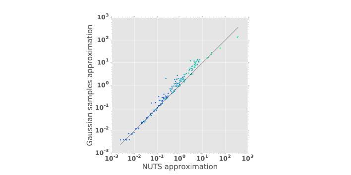
Figure 3: The two approximation of $KL(g_{LAP},f)$ are similar. As explained in the text, two numerical approximations of the KL divergence were considered. The difference was the computation of the normalization constant $\log(Z_{f})$. This figure corresponds to a simple scatter plot of both approximations, superposed with the identity line. Colors are the same as in Fig.1 and Fig.2. The results presented in the main text relied on the NUTS approximation.

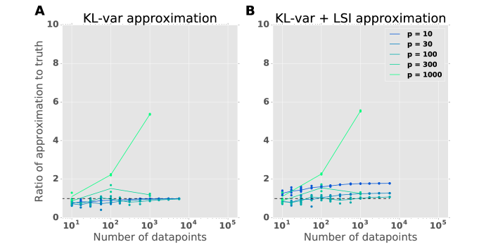
Figure 4: Evolution of the KL-var and "KL-var + LSI" approximations with $n$, when measured with respect to the other numerical approximation of $KL(g_{LAP},f)$. Panels A and B as in Fig.2. The behavior is qualitatively similar as in Fig.2.

F.3 Additional figures

Due to space constraints, we present here the evolution of the other approximations suggested by Cor.7.

We also present the evolution of the quality of the approximations as a function of the true KL divergence $KL\left(g_{LAP},f\right)$.

Evolution of the ratio "approximation of KL / KL" for all approximations proposed in Cor.7. A: KL-var approximation (repeated from Fig.2). B: "KL-var + LSI" approximation (repeated from Fig.2). C: "var ELBO + LSI" approximation. Note that due to the computational costs associated with this approximation, it was not computed for larger values of $p$ and $n$. D,E: Taylor approximations to third order of the KL-var and "KL-var + LSI" approximations. F,G: Taylor approximations to fourth order of the KL-var and "KL-var + LSI" approximations. Please note the change of scale in panels F and G. The Taylor approximations severely overestimate the true KL divergence for small values of $n$ and only become correct as $n$ is high enough. Note that due to computational constraints associated with computing large tensors, the Taylor approximations were not computed for the largest values of $p$.

Evolution of the ratio "approximation of KL / KL" for all approximations proposed in Cor.7 but as a function of the true KL divergence. All panels as in Supplementary Fig.F.3. Once again, note the change of scale in panels F and G. This representation shows that the KL-var approximation, and the other approximations proposed in Cor.7 are consistently tight whenever the true KL divergence is low and that they are otherwise upper-bounds. Further investigations are required in order to determine whether it is possible to prove that this relationship holds in a wider variety of situations.

References

• Metropolis etΒ al. [1953] Nicholas Metropolis, AriannaΒ W Rosenbluth, MarshallΒ N Rosenbluth, AugustaΒ H Teller, and Edward Teller. Equation of state calculations by fast computing machines. The journal of chemical physics, 21(6):1087–1092, 1953.
• Hastings [1970] WΒ Keith Hastings. Monte carlo sampling methods using markov chains and their applications. 1970.
• Brooks etΒ al. [2011] Steve Brooks, Andrew Gelman, Galin Jones, and Xiao-Li Meng. Handbook of markov chain monte carlo. CRC press, 2011.
• Blei etΒ al. [2017] DavidΒ M Blei, Alp Kucukelbir, and JonΒ D McAuliffe. Variational inference: A review for statisticians. Journal of the American Statistical Association, 112(518):859–877, 2017.
• Laplace [1820] PierreΒ Simon Laplace. ThΓ©orie analytique des probabilitΓ©s. Courcier, 1820.
• Opper and Archambeau [2009] Manfred Opper and CΓ©dric Archambeau. The variational gaussian approximation revisited. Neural computation, 21(3):786–792, 2009.
• Nickisch and Rasmussen [2008] Hannes Nickisch and CarlΒ Edward Rasmussen. Approximations for binary gaussian process classification. Journal of Machine Learning Research, 9(Oct):2035–2078, 2008.
• Bardenet etΒ al. [2014] RΓ©mi Bardenet, Arnaud Doucet, and Chris Holmes. Towards scaling up markov chain monte carlo: an adaptive subsampling approach. In International Conference on Machine Learning (ICML), pages 405–413, 2014.
• Chen etΒ al. [2014] Tianqi Chen, Emily Fox, and Carlos Guestrin. Stochastic gradient hamiltonian monte carlo. In International Conference on Machine Learning, pages 1683–1691, 2014.
• Maclaurin and Adams [2015] Dougal Maclaurin and RyanΒ Prescott Adams. Firefly monte carlo: Exact mcmc with subsets of data. In Twenty-Fourth International Joint Conference on Artificial Intelligence, 2015.
• Bardenet etΒ al. [2017] RΓ©mi Bardenet, Arnaud Doucet, and Chris Holmes. On markov chain monte carlo methods for tall data. The Journal of Machine Learning Research, 18(1):1515–1557, 2017.
• VanΒ der Vaart [2000] AadΒ W VanΒ der Vaart. Asymptotic statistics, volumeΒ 3. Cambridge university press, 2000.
• Kleijn etΒ al. [2012] BJK Kleijn, AWΒ VanΒ der Vaart, etΒ al. The bernstein-von-mises theorem under misspecification. Electronic Journal of Statistics, 6:354–381, 2012.
• Dehaene [2017] GuillaumeΒ P Dehaene. Computing the quality of the laplace approximation. Advance in Approximate Bayesian Inference: NEURIPS 2017 workshop, 2017.
• Saumard and Wellner [2014] Adrien Saumard and JonΒ A Wellner. Log-concavity and strong log-concavity: a review. Statistics surveys, 8:45, 2014.
• Bernstein [1911] SΒ Bernstein. Theory of probability. Kharkov, Moscow, 1911.
• von Mises [1931] Richard von Mises. Wahrscheinlichkeitsrechnung und ihre Anwendung in der Statistik und theoretischen Physik. Mary S. Rosenberg, 1931.
• Doob [1949] JosephΒ L Doob. Application of the theory of martingales. Le calcul des probabilites et ses applications, pages 23–27, 1949.
• Bakry and Γ‰mery [1985] Dominique Bakry and Michel Γ‰mery. Diffusions hypercontractives. In SΓ©minaire de ProbabilitΓ©s XIX 1983/84, pages 177–206. Springer, 1985.
• Otto and Villani [2000] Felix Otto and CΓ©dric Villani. Generalization of an inequality by talagrand and links with the logarithmic sobolev inequality. Journal of Functional Analysis, 173(2):361–400, 2000.
• Hillar and Lim [2013] ChristopherΒ J Hillar and Lek-Heng Lim. Most tensor problems are np-hard. Journal of the ACM (JACM), 60(6):45, 2013.
• Nocedal and Wright [2006] Jorge Nocedal and StephenΒ J Wright. Numerical optimization, chapter 3. Operations Research and Financial Engineering. Springer, New York, 2:30–65, 2006.
• Jones etΒ al. [2001–] Eric Jones, Travis Oliphant, Pearu Peterson, etΒ al. SciPy: Open source scientific tools for Python, 2001–. URL http://www.scipy.org/. [Online; accessed <today>].
• Hoffman and Gelman [2014] MatthewΒ D Hoffman and Andrew Gelman. The no-u-turn sampler: adaptively setting path lengths in hamiltonian monte carlo. Journal of Machine Learning Research, 15(1):1593–1623, 2014.
• Pereyra [2016] Marcelo Pereyra. Approximating bayesian confidence regions in convex inverse problems. In 2016 IEEE Statistical Signal Processing Workshop (SSP), pages 1–5. IEEE, 2016.
• Mortici [2010] Cristinel Mortici. New approximation formulas for evaluating the ratio of gamma functions. Mathematical and Computer Modelling, 52(1-2):425–433, 2010.