Robust and accurate computational estimation of the polarizability tensors of macromolecules

Abstract

Alignment of molecules through electric fields minimizes the averaging over orientations, e. g., in single-particle-imaging experiments. The response of molecules to external ac electric fields is governed by their polarizability tensor, which is usually calculated using quantum-chemistry methods. These methods are not feasible for large molecules. Here, we calculate the polarizability tensor of proteins using a regression model that correlates the polarizabilities of the 20 amino acids with perfect conductors of the same shape. The dielectric constant of the molecules could be estimated from the slope of the regression line based on Clausius–Mossotti equation. We benchmark our predictions against the quantum-chemistry results for the Trp cage mini protein and the measured dielectric constants of larger proteins. Our method has applications in computing laser-alignment of macromolecules, for instance, benefiting single particle imaging, as well as for the estimation of the optical and electrostatic characteristics of proteins and other macromolecules.

TOC Graphic

One of the main challenges in single particle imaging is recovering the orientation of the imaged particle from the sparse data in an individual diffraction pattern. It was proposed to use sophisticated computer algorithms to classify patterns accordingly, but these are highly dependent on the amount and quality of the available data Ayyer et al. (2016). Alternatively, the molecules can be aligned or oriented by an external field before they are imaged Spence and Doak (2004); Filsinger et al. (2011); Barty, Küpper, and Chapman (2013). For small molecules, this was demonstrated to enable experimental averaging of molecular-frame diffraction signals from hundred-thousands of shots Hensley, Yang, and Centurion (2012); Küpper et al. (2014); Stern et al. (2014), whereas for large macromolecules currently achievable degrees of alignment and orientationHolmegaard et al. (2009); Nevo et al. (2009); Chang et al. (2015); Karamatskos et al. (2018) would enable a strong reduction of the phase-space volume for orientational classification.

Molecules in the gas phase can be aligned and trapped in Stark-effect potentials using intense non-resonant laser pulses Friedrich and Herschbach (1995a); Stapelfeldt and Seideman (2003). At high frequency, this effect is dominated by the interactions between the induced dipole moment of the molecules and the electric field of the laser pulses. These interactions are characterized mainly by the molecules’ static polarizability and its anisotropy, which are described by the polarizability tensor of the molecule.

The molecular polarizability $\alpha$ is directly related to its electronic properties. It was shown that the polarizability is directly proportional to a molecule’s volume and inversely proportional to its ionization energy Brinck, Murray, and Politzer (1993). Furthermore, the value of $\alpha$ is related to the dielectric constant of the molecule by the Clausius–Mossotti relation and to its refractive index by the Lorentz–Lorenz equation Jansen (1958). For small molecules the correlation between the polarizability and molecular volume, ionization energy, electronegativity, and hardness was investigated extensively using ab-initio calculations and density functional theory (DFT) Brinck, Murray, and Politzer (1993); Blair and Thakkar (2014); Hohm and Thakkar (2011).

	$\alpha~{}(\text{\AA}^{3})$			$k$			$\alpha_{\parallel}~{}(\text{\AA}^{3})$			$\alpha_{\perp}~{}(\text{\AA}^{3})$			$\Delta{\alpha}~{}(\text{\AA}^{3})$			$\theta~{}(\,^{\circ})$
	$\alpha_{c}$	$\alpha_{m}$	$\alpha_{p}$	$k_{c}$	$k_{m}$	$k_{p}$	$\alpha_{\parallel{}c}$	$\alpha_{\parallel{}m}$	$\alpha_{\parallel{}p}$	$\alpha_{\perp{}c}$	$\alpha_{\perp{}m}$	$\alpha_{\perp{}p}$	$\Delta{\alpha{}c}$	$\Delta{\alpha{}m}$	$\Delta{\alpha{}p}$	$\theta_{m}$	$\theta_{c}$	$\theta_{pa}$
Gly	17	5	8	$0.19$	$0.11$	$0.09$	22	6	9	14	5	8	$8.25$	$1.23$	$2.33$	10	38	48
Ala	22	7	9	$0.15$	$0.09$	$0.07$	28	8	10	20	6	9	$7.95$	$1.62$	$2.31$	18	5	23
Ser	25	8	10	$0.1$	$0.07$	$0.05$	29	8	10	22	7	10	$6.53$	$1.38$	$2.2$	36	37	28
Pro	29	9	11	$0.12$	$0.06$	$0.06$	35	10	11	26	9	11	$9.29$	$1.1$	$2.41$	41	28	13
Val	33	10	12	$0.19$	$0.1$	$0.09$	44	12	13	28	10	12	$15.99$	$2.68$	$2.92$	5	3	5
Thr	31	9	11	$0.2$	$0.1$	$0.09$	41	11	13	26	9	11	$15.37$	$2.49$	$2.87$	24	20	7
Cys	28	10	11	$0.2$	$0.12$	$0.09$	38	12	12	23	8	10	$14.89$	$3.37$	$2.84$	30	27	6
Ile	40	12	14	$0.24$	$0.1$	$0.11$	58	15	17	31	11	13	$27.03$	$3.39$	$3.75$	6	10	8
Leu	40	10	14	$0.19$	$0.06$	$0.09$	56	11	16	33	10	13	$23.38$	$1.62$	$3.48$	34	15	22
Asn	34	10	12	$0.24$	$0.09$	$0.11$	50	11	15	26	9	11	$24.07$	$2.58$	$3.53$	38	36	2
Asp	32	11	12	$0.22$	$0.09$	$0.1$	45	12	14	25	10	11	$19.69$	$2.67$	$3.2$	41	40	1
Gln	41	12	14	$0.3$	$0.12$	$0.14$	66	14	18	29	10	12	$36.46$	$3.82$	$4.47$	24	31	10
Lys	44	12	15	$0.22$	$0.09$	$0.11$	64	15	18	34	11	14	$29.69$	$3.31$	$3.96$	8	24	15
Glu	40	14	14	$0.25$	$0.13$	$0.12$	61	17	17	30	12	12	$30.63$	$5.11$	$4.03$	29	38	9
Met	46	13	15	$0.37$	$0.15$	$0.17$	80	17	21	29	11	12	$51.16$	$5.93$	$5.58$	39	38	3
His	44	14	15	$0.31$	$0.15$	$0.15$	72	18	20	30	12	12	$41.92$	$6.1$	$4.88$	31	32	1
Phe	51	17	17	$0.33$	$0.18$	$0.15$	84	22	22	34	14	14	$49.44$	$8.13$	$5.45$	6	6	4
Arg	64	15	20	$0.4$	$0.16$	$0.18$	115	20	29	39	12	15	$76.2$	$7.04$	$7.48$	28	30	3
Tyr	56	18	18	$0.36$	$0.19$	$0.17$	96	24	25	36	14	14	$60.24$	$9.62$	$6.27$	4	4	4
Trp	64	22	20	$0.32$	$0.19$	$0.15$	103	28	26	44	18	16	$59.06$	$10.18$	$6.18$	2	19	17
C60	129	78	37	$0.0$	$0.0$	$0.01$	129	78	32	129	78	41	$0.0$	$0.0$	$1.71$	-	-	-
Trp cage	837	216	220	$0.16$	$0.04$	$0.08$	1048	232	235	732	208	213	$315.53$	$24.09$	$25.6$	15	7	8
PSII	3.6e5	–	1.0e5	$0.23$	–	$0.11$	5.2e5	–	1.0e5	2.8e5	–	1.2e5	$2.4e5$	–	$3.0e4$	–	37	–

Table 1: Polarizability parameters for the full set of molecules from ab initio calculations and the model developed in this work. The molecules are sorted according to their molecular weight. $\alpha$, $k$, $\alpha_{\parallel}$, $\alpha_{\perp}$, and $\Delta\alpha$ are defined according to (1)–(5), respectively. The subscripts $m,c,p$ depicts parameters calculated using DFT, calculated using ZENO, and predicted based on the regression model, respectively. $\theta_{m}$ and $\theta_{c}$ are the angles between the principle axis of inertia and the most polarizable axis calculated with DFT and ZENO, respectively. $\theta_{pa}$ is the angle between the most polarizable axes as calculated with DFT and ZENO. C₆₀ was explicitely included as a case not covered by our basis set, see text for details. No angles are reported for C₆₀, which has icosahedral symmetry and is a spherical top. DFT values for photosystem II (PS II) were not calculated.

In principle, the polarizability tensor can easily be calculated using standard quantum-chemistry packages. However, to avoid these often expensive calculations, semiempirical methods have been employed to calculate molecular polarizabilities from atomic polarizabilities. These calculations show that the orientation of the anisotropic atomic polarizabilities lies along the bond’s direction and it obeys a distance-dependent function for the polarizabilities in the direction of the unbound atoms Miller (1990). Another empirical study showed that the average molecular polarizability depends on the hybridization of the atoms’ orbitals, but not on the type of atoms Miller and Savchik (1979), i. e., the same atom would have different contributions to the molecular polarizability depending on its coordination.

Currently, calculating the molecular-polarizability tensor(s) for large molecules is challenging, as it requires expensive computational resources. Here, we provide a fast and reliable method for calculating the static-polarizability tensor of macromolecules. First, the polarizability tensor of a perfect conductor of the molecule’s shape is calculated by solving Laplace’s equation with Dirichlet boundary conditions and using Monte-Carlo-path-integral methods Mansfield, Douglas, and Garboczi (2001). Then, the Clausius–Mossotti relationship is used to relate these polarizabilities to the corresponding molecular polarizabilities through a linear regression model. In the current demonstration of this approach, we aim at specifically predicting the polarizability tensor of biological macromolecules, such as proteins, based on the polarizabilities of the 20 amino acids specified in Tab. 1 . The model is benchmarked against the Trp cage mini protein and we compare the resulting dielectric constant $\epsilon_{r}^{\text{comp}}$ to the measured $\epsilon_{r}^{\text{exp}}$ of larger proteins Kukic et al. (2013). Furthermore, we provide a prediction of the polarizability tensor of the prototypical large protein complex photosystem II.

Based on the principal moments of polarizability $\alpha_{ii}$, $i=1,2,3$, the average molecular polarizability $\alpha$ and the polarizability anisotropy $k$ are defined as following:

$$\alpha =\frac{\alpha_{11}+\alpha_{22}+\alpha_{33}}{3}$$ (1)

$$k =\sqrt{\frac{[(\alpha_{11}-\alpha)^{2}+(\alpha_{22}-\alpha)^{2}+(\alpha_{33}-\alpha)^{2}]}{6\alpha^{2}}}$$ (2)

In addition, it is instructive to calculate $\alpha_{\parallel}$ and $\alpha_{\perp}$ to “visualize” the polarizability ellipsoid as well as $\Delta{\alpha}$, which is the relevant quantity for the laser alignment of the most-polarizable axis (MPA) Friedrich and Herschbach (1995b):

$$\alpha_{\parallel} =\max\left(\alpha_{11},\alpha_{22},\alpha_{33}\right)$$ (3)

$$\alpha_{\perp} =\left(3\alpha-\alpha_{\parallel}\right)/2$$ (4)

$$\Delta{\alpha} =\alpha_{\parallel}-\alpha_{\perp}$$ (5)

Furthermore, to identify the orientation of the molecules’ structures with respect to their polarizability frame, we calculated the angle $\theta$ between the MPA and the molecular $a$ axis, i. e., the principal axis of inertia with the smallest moment of inertia, i. e., largest rotational constant, see Tab. 1 .

To build the regression model, the polarizability tensors of 20 amino acids were calculated using standard quantum-chemistry approaches, i. e., density-functional theory (DFT) starting from single-conformer structures obtained from New York University’s MathMol database NYU/ACF Scientific Visualization laboratory (2009), using the 6-31G($d,p$) basis set, the B3LYP functional, and the Gaussian 09 Frisch et al. software package. Then, 20 perfect conductors of the shapes of the amino acids were constructed by spheres corresponding to the respective van-der-Waals radii of the constituent atoms. The software ZENO Juba et al. (2017) was used to calculate the polarizability tensor for these perfect conductors by solving Laplace equation using Monte Carlo numerical-path integration Mansfield, Douglas, and Garboczi (2001). We used 1 million Monte Carlo steps for all calculations. We tested the effect of increasing the number of steps for tryptophan and alanine, using 100 million steps, and no significant differences were observed, i. e., the differences between the calculated polarizabilities were smaller than $0.5~{}\%$. The correlation is studied for $\alpha$, $k$, $\alpha_{\parallel}$, $\alpha_{\perp}$ and $\Delta\alpha$. The values of the average polarizabilities and the polarizability anisotropies for both approaches are tabulated in Tab. 1 .

The analytical relationship between the molecular polarizability $\alpha_{m}$ and polarizabilities of the perfect conductors $\alpha_{c}$ could be identified through the Clausius–Mossotti relation:

$$\lim_{\epsilon_{r}\rightarrow\infty}\frac{4\pi\alpha_{c}}{3V} =\frac{\epsilon_{r}-1}{\epsilon_{r}+2}$$ (6)

$$\Rightarrow\alpha_{c} =\frac{3V}{4\pi}$$ (7)

with the conductor’s polarizability $\alpha_{c}$, its volume $V$, and its dielectric constant $\epsilon_{r}$. For a molecule that has the same shape, but a finite dielectric constant, the molecular polarizability $\alpha_{m}$ is:

$$\frac{4\pi\alpha_{m}}{3V}=\frac{\epsilon_{r}-1}{\epsilon_{r}+2}$$ (8)

Substituting (7) in (8) yields:

$$\alpha_{m}=\alpha_{c}\frac{\epsilon_{r}-1}{\epsilon_{r}+2}$$ (9)

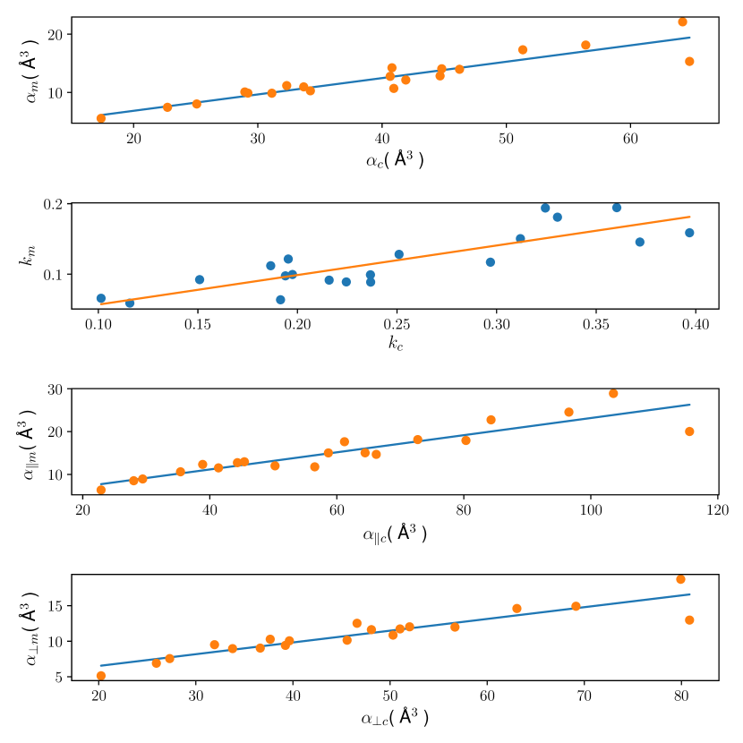
Figure 1: Correlations between a) the average molecular polarizabilities and the polarizabilities of same-shape conductors (in ų) for the 20 amino acids, b) the polarizability anisotropy, c) $\alpha_{\parallel}$, and d) $\alpha_{\perp}$. The raw data are presented in Tab. 1 ; see text for details, e. g., the parameters obtained from the linear regression.

The correlations between the molecular polarizability, e. g., computed quantum chemically, and the polarizability of a perfect conductor of the same shape, calculated with ZENO, for the 20 amino acids are shown in Fig. 1 for $\alpha$, $k$, $\alpha_{\parallel}$, and $\alpha_{\perp}$, respectively. The polarizabilities obtained from the quantum-chemistry calculations were significantly lower than the values for the perfect conductors, see Fig. 1 and Tab. 1 . However, the polarizability showed a strong correlation between the values from the two methods, which we analyzed through linear regressions of the individual pairs $(j_{m},j_{c})$ for $j=\alpha,k,\alpha_{\parallel},\alpha_{\perp}$. For the average polarizability $\alpha$ a slope $s_{\alpha}=0.28$ was obtained with a correlation coefficient $R_{\alpha}=0.92$ and, similarly, $s_{k}=0.42$ with $R_{k}=0.85$, $s_{\alpha_{\parallel}}=0.20$ with $R_{\alpha_{\parallel}}=0.92$, and $s_{\alpha_{\perp}}=0.42$ with $R_{\alpha_{\perp}}=0.93$. We crosschecked our model against the larger 6-311G($3df,3pd$) basis set for all amino acids and obtained practically the same correlation. According to (9) the slope $s_{\alpha}=(\epsilon_{r}-1)/(\epsilon_{r}+2)$ yields a dielectric constant $\epsilon_{r,\text{p}}=2.17$ averaged over the 20 amino acids.

Using the regression model that includes only the amino acids to predict the molecular polarizability of the Trp cage mini protein, using the PDB structure 1L2Y Neidigh, Fesinmeyer, and Andersen (2002), we predict a value of $\alpha_{p}=234$, which is 8 % larger than the value $\alpha_{m}=216$ from the quantum-chemistry calculation. Considering that this prediction takes a few seconds, in a single-core calculation, whereas the DFT quantum-chemistry calculations take more than 48 h on 24 cores on the same computer, this good agreement is extremely satisfying.

Adding the Trp cage data to the regression model of the average polarizability $\alpha$ the correlation coefficient increases to $R_{\alpha}=0.998$, the slope decreases to $s_{\alpha}=0.26$ and the resulting dielectric constant decreases to $\epsilon_{r,\text{p}}=2.05$. The predicted polarizabilities $\alpha_{\text{p}}$ and anisotropy components $k_{\text{p}},\alpha_{\parallel\text{p}},\alpha_{\perp\text{p}}$ based on the regression model are given in Tab. 1 .

To analyze the limits of our model, we used it to predicted the properties of C₆₀. The predicted $\epsilon_{r,\text{p}}=5.1$ is in fair agreement with the experimental value $\epsilon_{r,\text{exp}}=4.4(2)$ Hebard et al. (1991). However, there are large differences between the predicted $\alpha$, $\alpha_{\parallel}$ and $\alpha_{\perp}$ and the quantum-chemistry values for $C_{60}$. This can be attributed to the fact that our model basis does not contain similar molecules in terms of shape and composition and this comparison is instructive in setting the limitations of such a basis-set based model, i. e., it is clear that a different basis set is required to predict the properties of fullerenes.

protein	$\epsilon_{r,\text{exp}}$	$\epsilon_{r,\text{p}}$
ACBP	3.5 / 3.0	2.9
Av.Pc	2.5 / 3.0	3.3
P.1 Pc	2.0 / 2.5	2.9
hGRx	2.0 / 2.0	2.3

Table 2: Dielectric constants of different proteins from ref. Kukic et al., 2013, see text for specification, PDB numbers, and details. The two experimental values specify results from alternative analyses [Kukic et al., 2013]. Predicted values $\epsilon_{r,\text{p}}$ were obtained through (9).

For large proteins quantum-chemistry calculations of the polarizabilities are not feasible. Thus, we compare predictions from our model to experimental dielectric constant, see Tab. 2 . We have performed this comparison for the Acyl-CoA binding protein (ACBP), Plastocyanin from Anabaena variabilis (Av.Pc), Plastocyanin from Phormidium laminosum (P.1 Pc), and Human Glutaredoxin(hGRx); these structures were obtained from the protein data bank with PDB codes 1HB6 Van Aalten et al. (2001), 2GIM Schmidt, Christensen, and Harris (2006), 2Q5B Fromme et al. (2007), and 1JHB Sun, Berardi, and Bushweller (1998), respectively. The experimental values of $\epsilon_{r,\text{exp}}$ were obtained by solving the Poisson-Boltzmann equation (PBE) for an ensemble of crystal structures with the dielectric constant that reproduce the measured $pK_{a}$ values of a set of amino acids Kukic et al. (2013). The retrieved $\epsilon_{r}$ of these proteins varies with the number of structures used in solving the PBE and with the number of observed or absent NMR-chemical-shift perturbations (CSPs) associated with each ionizable group. In context, our predicted values are in a good agreement with these experiment-based values. This prediction of proper dielectric constants $\epsilon_{r}$ of proteins is essential for the understanding of electrostatic interactions inside proteins, which has substantial effects on the calculations of their physicochemical properties such as the refractive indices $n$ as well as their $pK_{a}$s and midpoint potentials $E_{m}$ Gilson et al. (1985). Thus, we point out that the accuracy of such protein properties could be explored using estimated dielectric constant according to the approach we present here, instead of using a constant value for all proteins Ullmann and Bombarda (2013).

Regarding laser alignment, e. g., for molecular-frame single-particle imaging, the molecular polarizability anisotropy defines the rotational dynamics in external electric fields. We have calculated the polarizability anisotropies $k$ and $\Delta\alpha$ as well as the parallel $\alpha_{\parallel}$ and perpendicular components $\alpha_{\perp}$ of the polarizability according to equations (2)–(4). The resulting values are given in Tab. 1 and Fig. 1 . Also for these properties there are strong correlations between the quantum-chemically calculated molecular properties and the values for a perfect conductor of the same shape. Utilizing the slopes determined from a linear regression we predict the values $k_{p}$, $\alpha_{\parallel_{p}}$, $\alpha_{\perp_{p}}$, and $\Delta\alpha$, see Tab. 1 . In comparison to quantum-chemistry values we obtained standard deviations of 0.02 Å³, 2.3 Å³, 1.1 Å³, and 2.7 Å³, respectively for the set of the 20 amino acids and Trp cage, which reflects the good agreement of our model to the DFT calculations. Furthermore, we checked the agreement of the angles between the MPA and the molecules’ inertial $a$ axis, see Tab. 1 , which also has a significant influence on the rotational dynamics in the laser alignment of complex molecules Hansen et al. (2013). The average of the angles between the predicted and the DFT MPA is $13\,^{\circ}$, with a standard deviation of $14\,^{\circ}$. In general, the largest deviations are observed for small amino acids, which we ascribe to their highly anisotropic distribution of atoms around the axes of inertia. However, for large molecules such as Trp cage this effect reduces significantly. Thus, for macromolecules, the polarizability tensors of the perfect conductors have orientations in the molecules’ inertial frame that are fairly similar to the quantum-chemically calculated once. This indicates that the calculated rotational/alignment dynamics using values predicted from our model will reflect the actual molecular dynamics well. We have started such calculations to predict achievable degrees of alignment for large macromolecules. These should reliably predict the achievable degrees of alignment of large and complex macromolecules and could be exploited for angular deconvolution of diffractive-imaging data.

In conclusion, we devised a simple model for the prediction of the static-polarizability tensors of large or complex molecules based on extremely fast and robust calculations of the polarizability tensor of the corresponding conductor of the same shape. We benchmarked this model for proteins as prototypical biological macromolecules using a basis set of 20 amino acids. Furthermore, using the Clausius-Mosotti equation these results were extended to predictions of the macromolecules’ dielectric constants. The accuracy of the predicted polarizabilities and anisotropies, compared to values from standard quantum-chemistry calculations, is better than 10 % and the predicted dielectric constants are within the error bounds of the experimental values.

These results have important applications in the computational prediction and the quantitative understanding of laser alignment of macromolecules, e. g., in single-molecule diffractive imaging experiments, as well as for calculations of the $pK_{a}$ and $E_{m}$ values of proteins.

References

- Ayyer et al. (2016) K. Ayyer, T.-Y. Lan, V. Elser, and N. D. Loh, “Dragonfly: an implementation of the expand–maximize–compress algorithm for single-particle imaging,” J. Appl. Cryst. 49, 1320–1335 (2016).
- Spence and Doak (2004) J. C. H. Spence and R. B. Doak, “Single molecule diffraction,” Phys. Rev. Lett. 92, 198102 (2004).
- Filsinger et al. (2011) F. Filsinger, G. Meijer, H. Stapelfeldt, H. Chapman, and J. Küpper, “State- and conformer-selected beams of aligned and oriented molecules for ultrafast diffraction studies,” Phys. Chem. Chem. Phys. 13, 2076–2087 (2011), arXiv:1009.0871 [physics] .
- Barty, Küpper, and Chapman (2013) A. Barty, J. Küpper, and H. N. Chapman, “Molecular imaging using x-ray free-electron lasers,” Annu. Rev. Phys. Chem. 64, 415–435 (2013).
- Hensley, Yang, and Centurion (2012) C. J. Hensley, J. Yang, and M. Centurion, “Imaging of isolated molecules with ultrafast electron pulses,” Phys. Rev. Lett. 109, 133202 (2012).
- Küpper et al. (2014) J. Küpper, S. Stern, L. Holmegaard, F. Filsinger, A. Rouzée, A. Rudenko, P. Johnsson, A. V. Martin, M. Adolph, A. Aquila, S. Bajt, A. Barty, C. Bostedt, J. Bozek, C. Caleman, R. Coffee, N. Coppola, T. Delmas, S. Epp, B. Erk, L. Foucar, T. Gorkhover, L. Gumprecht, A. Hartmann, R. Hartmann, G. Hauser, P. Holl, A. Hömke, N. Kimmel, F. Krasniqi, K.-U. Kühnel, J. Maurer, M. Messerschmidt, R. Moshammer, C. Reich, B. Rudek, R. Santra, I. Schlichting, C. Schmidt, S. Schorb, J. Schulz, H. Soltau, J. C. H. Spence, D. Starodub, L. Strüder, J. Thøgersen, M. J. J. Vrakking, G. Weidenspointner, T. A. White, C. Wunderer, G. Meijer, J. Ullrich, H. Stapelfeldt, D. Rolles, and H. N. Chapman, “X-ray diffraction from isolated and strongly aligned gas-phase molecules with a free-electron laser,” Phys. Rev. Lett. 112, 083002 (2014), arXiv:1307.4577 [physics] .
- Stern et al. (2014) S. Stern, L. Holmegaard, F. Filsinger, A. Rouzée, A. Rudenko, P. Johnsson, A. V. Martin, A. Barty, C. Bostedt, J. D. Bozek, R. N. Coffee, S. Epp, B. Erk, L. Foucar, R. Hartmann, N. Kimmel, K.-U. Kühnel, J. Maurer, M. Messerschmidt, B. Rudek, D. G. Starodub, J. Thøgersen, G. Weidenspointner, T. A. White, H. Stapelfeldt, D. Rolles, H. N. Chapman, and J. Küpper, “Toward atomic resolution diffractive imaging of isolated molecules with x-ray free-electron lasers,” Faraday Disc. 171, 393 (2014), arXiv:1403.2553 [physics] .
- Holmegaard et al. (2009) L. Holmegaard, J. H. Nielsen, I. Nevo, H. Stapelfeldt, F. Filsinger, J. Küpper, and G. Meijer, “Laser-induced alignment and orientation of quantum-state-selected large molecules,” Phys. Rev. Lett. 102, 023001 (2009), arXiv:0810.2307 [physics] .
- Nevo et al. (2009) I. Nevo, L. Holmegaard, J. H. Nielsen, J. L. Hansen, H. Stapelfeldt, F. Filsinger, G. Meijer, and J. Küpper, “Laser-induced 3D alignment and orientation of quantum state-selected molecules,” Phys. Chem. Chem. Phys. 11, 9912–9918 (2009), arXiv:0906.2971 [physics] .
- Chang et al. (2015) Y.-P. Chang, D. A. Horke, S. Trippel, and J. Küpper, “Spatially-controlled complex molecules and their applications,” Int. Rev. Phys. Chem. 34, 557–590 (2015), arXiv:1505.05632 [physics] .
- Karamatskos et al. (2018) E. T. Karamatskos, S. Raabe, T. Mullins, A. Trabattoni, P. Stammer, G. Goldsztejn, R. R. Johansen, K. Długołęcki, H. Stapelfeldt, M. J. J. Vrakking, S. Trippel, A. Rouzée, and J. Küpper, “Molecular movie of ultrafast coherent rotational dynamics,” (2018), arXiv:1807.01034 .
- Friedrich and Herschbach (1995a) B. Friedrich and D. Herschbach, “Alignment and trapping of molecules in intense laser fields,” Phys. Rev. Lett. 74, 4623–4626 (1995a).
- Stapelfeldt and Seideman (2003) H. Stapelfeldt and T. Seideman, “Colloquium: Aligning molecules with strong laser pulses,” Rev. Mod. Phys. 75, 543–557 (2003).
- Brinck, Murray, and Politzer (1993) T. Brinck, J. Murray, and P. Politzer, “Polarizability and volume,” J. Chem. Phys. 98, 4305–4306 (1993).
- Jansen (1958) L. Jansen, “Molecular theory of the dielectric constant,” Phys. Rev. 112, 434–444 (1958).
- Blair and Thakkar (2014) S. Blair and A. Thakkar, “Relating polarizability to volume, ionization energy, electronegativity, hardness, moments of momentum, and other molecular properties,” J. Chem. Phys. 141, 074306 (2014).
- Hohm and Thakkar (2011) U. Hohm and A. Thakkar, “New relationships connecting the dipole polarizability, radius, and second ionization potential for atoms,” J. Phys. Chem. A 116, 697–703 (2011).
- Miller (1990) K. J. Miller, “Calculation of the molecular polarizability tensor,” J. Am. Chem. Soc. 112, 8543–8551 (1990).
- Miller and Savchik (1979) K. J. Miller and J. Savchik, “A new empirical method to calculate average molecular polarizabilities,” J. Am. Chem. Soc. 112, 7206–7213 (1979).
- Mansfield, Douglas, and Garboczi (2001) M. L. Mansfield, J. F. Douglas, and E. J. Garboczi, “Intrinsic viscosity and the electrical polarizability of arbitrarily shaped objects,” Phys. Rev. A 64, 061401–061416 (2001).
- Kukic et al. (2013) P. Kukic, D. Farrell, L. P. McIntosh, B. G.-M. E., K. S. Jensen, Z. Toleikis, K. Teilum, and J. E. Nielsen, “Protein dielectric constants determined from NMR chemical shift perturbations,” J. Am. Chem. Soc. 135, 16968–16976 (2013).
- Friedrich and Herschbach (1995b) B. Friedrich and D. Herschbach, “Polarization of molecules induced by intense nonresonant laser fields,” J. Phys. Chem. 99, 15686 (1995b).
- NYU/ACF Scientific Visualization laboratory (2009) NYU/ACF Scientific Visualization laboratory, “MathMol (Mathematics and Molecules),” New York University (2009), URL: https://www.nyu.edu/pages/mathmol.
- (24) M. J. Frisch, G. W. Trucks, H. B. Schlegel, G. E. Scuseria, M. A. Robb, J. R. Cheeseman, G. Scalmani, V. Barone, B. Mennucci, G. A. Petersson, H. Nakatsuji, M. Caricato, X. Li, H. P. Hratchian, A. F. Izmaylov, J. Bloino, G. Zheng, J. L. Sonnenberg, M. Hada, M. Ehara, K. Toyota, R. Fukuda, J. Hasegawa, M. Ishida, T. Nakajima, Y. Honda, O. Kitao, H. Nakai, T. Vreven, J. A. Montgomery, Jr., J. E. Peralta, F. Ogliaro, M. Bearpark, J. J. Heyd, E. Brothers, K. N. Kudin, V. N. Staroverov, R. Kobayashi, J. Normand, K. Raghavachari, A. Rendell, J. C. Burant, S. S. Iyengar, J. Tomasi, M. Cossi, N. Rega, J. M. Millam, M. Klene, J. E. Knox, J. B. Cross, V. Bakken, C. Adamo, J. Jaramillo, R. Gomperts, R. E. Stratmann, O. Yazyev, A. J. Austin, R. Cammi, C. Pomelli, J. W. Ochterski, R. L. Martin, K. Morokuma, V. G. Zakrzewski, G. A. Voth, P. Salvador, J. J. Dannenberg, S. Dapprich, A. D. Daniels, Ö. Farkas, J. B. Foresman, J. V. Ortiz, J. Cioslowski, and D. J. Fox, “Gaussian 09 Revision A.02,” Gaussian Inc. Wallingford CT 2009.
- Juba et al. (2017) D. Juba, D. J. Audus, M. Mascagni, J. F. Douglas, and W. Keyrouz, “ZENO: Software for calculating hydrodynamic, electrical, and shape properties of polymer and particle suspensions,” J. Res. Nat. Inst. Stand. Tech. 122, 20 (2017).
- Neidigh, Fesinmeyer, and Andersen (2002) J. Neidigh, R. Fesinmeyer, and N. Andersen, “Designing a 20-residue protein,” Nat.Struct.Mol.Biol. 9, 425–430 (2002).
- Hebard et al. (1991) A. F. Hebard, R. C. Haddon, R. M. Fleming, and A. R. Kortan, “Deposition and characterization of fullerene films,” Appl Phys Lett 59, 2109–2111 (1991).
- Van Aalten et al. (2001) D. Van Aalten, K. Milne, J. Zou, G. Kleywegt, T. Bergfors, M. Ferguson, J. Knudsen, and T. Jones, “Binding site differences revealed by crystal structures of plasmodium falciparum and bovine acyl-coa binding protein,” J. Mol. Biol. 309, 181–192 (2001).
- Schmidt, Christensen, and Harris (2006) L. Schmidt, H. Christensen, and P. Harris, “Structure of plastocyanin from the cyanobacterium anabaena variabilis,” Acta Cryst. B 62, 1022–1029 (2006).
- Fromme et al. (2007) R. Fromme, Y. Bukhman-DeRuyter, I. Grotjohann, H. Mi, and P. Fromme, “High resolution structure of plastocyanin from phormidium laminosum,” (2007).
- Sun, Berardi, and Bushweller (1998) C. Sun, M. Berardi, and J. Bushweller, “The NMR solution structure of human glutaredoxin in the fully reduced form,” J. Mol. Biol. 280, 687–701 (1998).
- Gilson et al. (1985) M. K. Gilson, A. Rashin, R. Fine, and B. Honig, “On the calculation of electrostatic interactions in proteins,” J. Mol. Biol. 184, 503–516 (1985).
- Ullmann and Bombarda (2013) G. M. Ullmann and E. Bombarda, “ values and redox potentials of proteins. what do they mean?” J. Biol. Chem. 394, 611––619 (2013).
- Hansen et al. (2013) J. L. Hansen, J. J. Omiste, J. H. Nielsen, D. Pentlehner, J. Küpper, R. González-Férez, and H. Stapelfeldt, “Mixed-field orientation of molecules without rotational symmetry,” J. Chem. Phys. 139, 234313 (2013), arXiv:1308.1216 [physics] .