Unified formalism for entropy productions and fluctuation relations

Abstract

Stochastic entropy production, which quantifies the difference between the probabilities of trajectories of a stochastic dynamics and its time reversals, has a central role in nonequilibrium thermodynamics. In the theory of probability, the change in the statistical properties of observables due to reversals can be represented by a change in the probability measure. We consider operators on the space of probability measure that induce changes in the statistical properties of a process, and formulate entropy productions in terms of these change-of-probability-measure (CPM) operators. This mathematical underpinning of the origin of entropy productions allows us to achieve an organization of various forms of fluctuation relations: All entropy productions have a non-negative mean value, admit the integral fluctuation theorem, and satisfy a rather general fluctuation relation. Other results such as the transient fluctuation theorem and detailed fluctuation theorems then are derived from the general fluctuation relation with more constraints on the operator of a entropy production. We use a discrete-time, discrete-state-space Markov process to draw the contradistinction among three reversals of a process: time reversal, protocol reversal and the dual process. The properties of their corresponding CPM operators are examined, and the domains of validity of various fluctuation relations for entropy productions in physics and chemistry are revealed. We also show that our CPM operator formalism can help us rather easily extend other fluctuations relations for excess work and heat, discuss the martingale properties of entropy productions, and derive the stochastic integral formulas for entropy productions in constant-noise diffusion process with Girsanov theorem. Our formalism provides a general and concise way to study the properties of entropy-related quantities in stochastic thermodynamics and information theory.

I Introduction

Stochastic thermodynamics is a milestone extending equilibrium statistical physics to the nonequilibrium realm, and could provide a general theory for emergent phenomena in mesoscopic systems (Searles and Evans, 1999; Jiang et al., 2004; Seifert, 2012; Qian, 2016; Thompson and Qian, 2016). It studies entropy productions (EPs), their relations to work and heat done by the system of interest (Crooks, 1998), their statistical properties such as expectations and martingale properties, and also how their probability density functions change after time reversals, called fluctuation theorems or fluctuation relations (FRs) Jarzynski (1997); Crooks (1999); Maes (2004); Seifert (2012).

Various distinct FRs for different EPs have been studied in various settings including discrete-time Markov chains (Qian, 2001a; Crooks, 1998, 2000; Riechers and Crutchfield, 2017), continuous-time Markov chains (Markov jump processes) (Lebowitz and Spohn, 1999; Ge and Qian, 2010; Esposito and Van den Broeck, 2010; Rao and Esposito, 2018; Ge, 2009; Seifert, 2005), diffusion processes (as stochastic differential equations or Langevin equations) (Hatano and Sasa, 2001; Kurchan, 1998; Qian, 2001b, a; Ge, 2009; Seifert, 2005; Chernyak et al., 2006), and even general stochastic processes Crooks (1999); Jiang et al. (2004); Ge and Jiang (2007); Ge (2009); Shargel (2010); Chétrite and Gupta (2011). To discuss a few, in (Crooks, 1999), Crooks’ fluctuation theorem for the total entropy production was introduced for systems with detailed balance and the conditions for it to hold was illustrated; in (Ge and Jiang, 2007), the dissipation function from Evans and Searles Evans and Searles (2002) was rigorously shown to generally admit the transient fluctuation theorem (TFT); in (Esposito and Van den Broeck, 2010), a detailed fluctuation theorem related to the involutive property of the change in probability (iDFT) was introduced but the correct condition for total entropy production and non-adiabatic entropy production was not stated; in (Seifert, 2012), the generalized Crooks’ fluctuation theorem for non-detail balanced systems (rDFT) and TFT for different EPs were discussed thoroughly for diffusion processes. iDFT was also discussed briefly; and in (García-García et al., 2012), rDFT was thoroughly discussed in general Markov processes for the three entropy productions except dissipation function.

The extensiveness of FTs calls for an unifying formalism to derive all FTs mentioned above in one general theory, organize their domain of validity comprehensively, and open ways to reveal more properties of EPs. It is suggested in Jiang et al. (2004); Ge and Jiang (2007); Ge (2009); Wojtkowski (2009); Shargel (2010); Chétrite and Gupta (2011) that measure-theoretic probability theory pioneered by A. N. Komogorov (Kolmogorov, 2018) will do the trick. One key is the understanding that EPs in physics are the fluctuating relative entropy for trajectories between the original process and the reversed process, with different EPs given by different reversals or composite of reversals Crooks (1998, 1999); Seifert (2012). In the measure-theoretic formalism, EP is thus mathematically expressed as the negative logarithm of the Radon-Nikodym Derivative (RND), which is a re-weighting factor in taking expectation to change a probability measure from the original one to the other. It is this mathematical underpinning that enables us to arrive an organization of FRs and further derive/recover other properties with a deeper understanding of EPs, e.g. their martingale properties Chétrite and Gupta (2011); Neri et al. (2017); Chétrite et al. (2019).

Our paper thus serves as a comprehensive overview on how to understand EPs and their statistical properties, primarily FRs, from measure-theoretic probability theory and our change-of-probability-measure (CPM) operator theory. We revisit discussions on different time reversals, their associated EPs in physics and chemistry, and derive various FRs from our general and concise approach. Our goal is to demonstrate that by adopting this CPM operator formalism, one can neatly derive many known results in the literature with more rigor and generality, achieve new understanding on EPs and FRs, and reveal more properties of EPs.

The outline of this paper is summarized below. In Section II, we briefly introduce measure-theoretic probability theory, the notion of CPM operator, and present general statistical properties for a general EP as a fluctuating relative entropy in general stochastic processes without Markovian assumption. With more constraints on the properties of the CPM operator, we deduce the general conditions for various known FRs and reveal a hierarchy of the domain of validity for various FRs with new relations recognized between them such as TFT$\Rightarrow$iDFT. In Section III, we further use a discrete-time Markov chain to illustrate the contradistinction of three different time reversals of the dynamics that are prominent in physics and chemistry. The involutive and commutative properties of their corresponding CPM operators are discussed.

In Section IV, we apply the results in the previous two sections to discuss the properties of the four EPs commonly considered in physics and chemistry. Notably, we discuss the difference between dissipation function and total entropy production and show that the two EPs have non-zero difference in expectation for finite time interval in time homogeneous processes but have the same entropy production rate in infinitesimal time interval. The two seemly contradicting results are resolved by noting the non-additivity of the dissipation function when connecting time intervals.

We further demonstrate how properties of EPs other than their FRs can be derived and extended in a rather straightforward way with this CPM operator formalism. We discuss the martingale properties of the four EPs which can lead to more statistics on the EPs Chétrite and Gupta (2011); Neri et al. (2017); Chétrite et al. (2019), and extend the so-called differential FR for work and heat (Jarzynski, 2000; Maragakis et al., 2008) to non-equilibrium systems at the end of Section IV. We also show how to use our CPM operator formalism and Girsanov theorem Jiang et al. (2004) to derive the stochastic integral formulas of the four EPs for general time inhomogeneous constant-noise diffusion processes in Section V. The notations for the five heavily-discussed FRs and the EPs involved in them are summarized in Table 1.

FR	definition	the EP involved	validity and sufficient conditions
GFR	$\mathbb{P}\left\{S_{\nu}\in\mathrm{d}s\right\}=e^{s}\mathbb{P}^{\nu}\left\{S_{\nu}\in\mathrm{d}s\right\}$	$S_{\nu}(\omega)=\ln\frac{\mathrm{d}\mathbb{P}\ \thinspace}{\mathrm{d}\mathbb{P}^{\nu}}(\omega)$	generally valid
IFT	$\mathbb{E}\left[e^{-S_{\nu}}\right]=1$
rDFT	$\mathbb{P}\left\{S_{\nu}(\omega)\in\mathrm{d}s\right\}=e^{s}\mathbb{P}^{\nu}\left\{\bar{S}_{\nu}(r(\omega))\in-\mathrm{d}s\right\}$	$\bar{S}_{\nu}(\omega)=\ln\frac{\mathrm{d}\mathbb{P}^{\mathrm{R}}\ \thinspace}{\mathrm{d}\mathbb{P}^{\mathrm{R}\nu}}(\omega)$	$\bar{S}_{\nu}(r(\omega))=-S_{\nu}(\omega)$
iDFT	$\mathbb{P}\left\{S_{\nu}(\omega)\in\mathrm{d}s\right\}=e^{s}\mathbb{P}^{\nu}\left\{\tilde{S}_{\nu}(\omega)\in-\mathrm{d}s\right\}$	$\tilde{S}_{\nu}(\omega)=\ln\frac{\mathrm{d}\mathbb{P}^{\nu}\thinspace\ }{\mathrm{d}\mathbb{P}^{\nu\nu}}(\omega)$	$\nu$ involutive on $\mathcal{P}$
TFT	$\mathbb{P}\left\{S_{\nu}(\omega)\in\mathrm{d}s\right\}=e^{s}\mathbb{P}\left\{S_{\nu}(\omega)\in-\mathrm{d}s\right\}$	$S_{\nu}(\omega)=\ln\frac{\mathrm{d}\mathbb{P}\ \thinspace}{\mathrm{d}\mathbb{P}^{\nu}}(\omega)$	$\nu$ realized by an
			involutive map on $\Omega$

Table 1: The five fluctuation relations (FRs) of the EP, $S_{\nu}$, with the CPM operator $\nu$ discussed in this paper. IFT is the integral fluctuation theorem Jarzynski (1997); GFR is the general FR in Equation (8c); TFT is the transient fluctuation theorem in (Kurchan, 1998; Evans and Searles, 2002; Ge and Jiang, 2007; Seifert, 2012), iDFT is the detailed fluctuation theorem in (Esposito and Van den Broeck, 2010), and rDFT is the generalization of Crooks’ fluctuation theorem (Seifert, 2012; Crooks, 1999; Chernyak et al., 2006; García-García et al., 2012). We have shown in the text that TFT implies iDFT. This summarizes the hierarchical structure of the validity of the five FRs.

Properties of the four EPs we have discussed primarily in this paper are also summarized in Table 2,

EP	$=0$ when	$\mathbb{E}[\cdot]\geq 0$, IFT, GFR	TFT	iDFT	rDFT	additive in time	$e^{-\left[\cdot\right]}$ a martingale
$S_{\mathrm{T}}=\ln\frac{\mathrm{d}\mathbb{P}\ \thinspace}{\mathrm{d}\mathbb{P}^{\mathrm{T}}}$	TH+SS+DB	Yes	Yes	Yes	TH+SS	TH+SS	TH+SS
$S_{\mathrm{tot}}=\ln\frac{\mathrm{d}\mathbb{P}\ \ \ }{\mathrm{d}\mathbb{P}^{\mathrm{RT}}}$	TH+SS+DB	Yes	TH+SS	TH+SS	if $P_{0}=P_{t}^{\mathrm{R}}$	Yes	TH+SS
$Q_{\mathrm{hk}}=\ln\frac{\mathrm{d}\mathbb{P}\ }{\mathrm{d}\mathbb{P}^{\dagger}}$	TH+DB	Yes	TH+SS	Yes	Yes	Yes	Yes
$S_{\mathrm{na}}=\ln\frac{\mathrm{d}\mathbb{P}\ \ \ \ }{\mathrm{d}\mathbb{P}^{\mathrm{R}\dagger\mathrm{T}}}$	TH+SS	Yes	TH+SS	TH+SS	if $P_{0}=P_{t}^{\mathrm{R}}$	Yes	TH+SS

Table 2: Properties of the four entropy productions (EPs) for Markov Processes. $S_{\mathrm{T}}$ is the dissipation function (Evans and Searles, 2002; Seifert, 2012); $S_{\mathrm{tot}}$ is the total EP (Harris and Schutz, 2007; Esposito and Van den Broeck, 2010; Seifert, 2012; Ge and Qian, 2010); $Q_{\mathrm{hk}}$ is the housekeeping heat (Seifert, 2012; Ge and Qian, 2010) or called the adiabatic EP in (Esposito and Van den Broeck, 2010); and $S_{\mathrm{na}}$ is the non-adiabatic EP (Esposito and Van den Broeck, 2010). $\mathbb{E}[\cdot]$ denotes the expectation and the non-negative expectation of entropy production is the classical second law of thermodynamics. $P_{0}$ is the initial distribution of the original process. $P_{t}^{\mathrm{R}}$ is the terminal distribution of the protocol reversed process, i.e. the distribution one gets by starting with initial distribution $P_{t}$ and then marching with reversed order of transition proability matrices for $t$ steps. TH stands for time homogeneous; SS stands for steady state; and DB means the steady state has detailed balance. Note that when TH and SS, i.e. when the system is in nonequilibrium steady state, we have $S_{\mathrm{T}}\equiv S_{\mathrm{tot}}\equiv Q_{\mathrm{hk}}$ and $S_{\mathrm{na}}=0$.

. Finally, in Section VI, we discuss possible future extensions of our work.

II General Theory

To describe stochastic processes with a measure-theoretic probability theory, we start by specifying a tuple $\left(\Omega,\mathcal{F}\right)$ called measurable space where the sample space $\Omega$ collects all possible trajectories $\omega$ and the $\sigma$-algebra $\mathcal{F}$ collects all events of interest. Physical quantities, as observables, are then random variables defined on $\left(\Omega,\mathcal{F}\right)$ (Qian, 2001b). The statistical properties of a stochastic process are further specified by a probability space $\left(\Omega,\mathcal{F},\mathbb{P}\right)$ with a probability measure $\mathbb{P}$ that assigns probabilities to events of interest in $\mathcal{F}$. See Appendix A for more thorough introduction.

The collection of all possible probability measures on a given measurable space $\left(\Omega,\mathcal{F}\right)$ forms an affine space of probability measures $\mathcal{P}$ (Hong et al., 2019). Each probability measure $\mathbb{P}\in\mathcal{P}$ corresponds to a stochastic process with specific statistical properties . In this paper, we would assume $\mathcal{P}$ collects probability measures that are absolutely continuous to each other (also called equivalent in probability theory), i.e. if an event has zero probability for a stochastic process $\mathbb{P}\in\mathcal{P}$, the event has zero probability under all $\mathbb{P}$ in $\mathcal{P}$.

II.1 Change of Probability Measure

With the statistical properties of stochastic processes specified by probability measures $\mathbb{P}\in\mathcal{P}$, the difference between the statistical properties of two processes is characterized by a change of probability measure (CPM) $\mathbb{P}\rightarrow\mathbb{P}^{\nu}\in\mathcal{P}$, which induces changes in the statistical properties of observables. This change in statistical properties can be mathematically represented by a random variable called the Radon-Nikodym Derivative (RND), denoted as $\frac{\mathrm{d}\mathbb{P}^{\nu}}{\mathrm{d}\mathbb{P}\ }(\omega)$ (Hong et al., 2019; Qian et al., 2019). Intuitively, RND serves as a re-weighting factor in taking expectation. For an arbitrary random variable $Y(\omega)$ defined on $\left(\Omega,\mathcal{F}\right)$, it’s expectation under $\mathbb{P}^{\nu},$ denoted as $\mathbb{E}^{\nu}[Y(\omega)]$, can be expressed by the reweighting factor and the previous expectation $\mathbb{E}[\cdot]$,

$$\mathbb{E}^{\nu}[Y(\omega)]=\mathbb{E}[Y(\omega)\frac{\mathrm{d}\mathbb{P}^{\nu}}{\mathrm{d}\mathbb{P}\ \thinspace}(\omega)].$$ (1)

Note that to get the probability density function of a random variable $X(\omega)$, we can let $Y(\omega)$ to be an indicator function of $X(\omega)$ taking values in between $x$ and $x+\mathrm{d}x$ (denoted as $X(\omega)\in\mathrm{d}x$ for simplicity). That is,

$$\mathbb{P}^{\nu}\{X(\omega)\in\mathrm{d}x\} =\mathbb{E}^{\nu}[\mathbb{I}_{\left\{\omega:X(\omega)\in\mathrm{d}x\right\}}]$$ (2a)

$$=\mathbb{E}[\mathbb{I}_{\left\{\omega:X(\omega)\in\mathrm{d}x\right\}}\frac{\mathrm{d}\mathbb{P}^{\nu}}{\mathrm{d}\mathbb{P}\ \thinspace}(\omega)]$$ (2b)

with the indicator function $$\mathbb{I}_{A}(\omega) \omega A$$ returning 1 if is in the event and returning 0 otherwise. Throughout the paper, we use capitalized letters for random variables and their corresponding lower letters for their values for a specific realization.

CPM and RND are key concepts in the theory of fluctuating entropy and EP (Qian, 2001b; Seifert, 2005; Qian et al., 2019). For systems with a discrete sample space $\Omega$ (trajectory space when considering processes), RND reduces to the ratio of two probability mass functions, and for those with continuous sample spaces, it reduces to the ratio of two probability density functions. In either cases, the RND is obtained from the ratio, which is defined on the codomain of a random variable, with random variables plugged back in (Qian et al., 2019).

In stochastic thermodynamics, a physical operation such as a time reversal in the dynamics is an operation that changes the probability measure $\mathbb{P}\in\mathcal{P}$ to a new probability measure $\mathbb{P}^{\nu}\in\mathcal{P}$ based on $\mathbb{P}$ alone. This means we are interested in a transformation $\nu$ on the space of all probability measures $\mathcal{P}\to\mathcal{P}$, and for each given measure $\mathbb{P}\in\mathcal{P}$, a physical operation defines a RND that is dependent upon the current process $\left(\Omega,\mathcal{F},\mathbb{P}\right)$. Thus, we consider operators $\nu$ that operates on $\mathbb{P}$, giving every measure $\mathbb{P}\in\mathcal{P}$ an image $\mathbb{P}^{\nu}\in\mathcal{P}$ and a corresponding RND. The new probability measure $\mathbb{P}^{\nu}$ is obtained by

$$\mathbb{P}^{\nu}\left\{A\right\}\coloneqq\mathbb{E}\left[\frac{\mathrm{d}\mathbb{P}^{\nu}}{\mathrm{d}\mathbb{P}\ \thinspace}\mathbb{I}_{A}\right],$$ (3)

$\forall A\in\mathcal{F}$ and $\forall\mathbb{P}\in\mathcal{P}$.

As we shall show, only very special operator $\nu$ defined on $\mathcal{P}$ can be represented as a result of a map $\mu$ from $\Omega$ to $\Omega$. In those special cases, the map $\mu$ maps an event of interest $A\in\mathcal{F}$ to another, $\mu(A)\in\mathcal{F}$, which is obtained by replacing all the $\omega$s in $A$ by the $\mu(\omega)$s, e.g. if $A=\omega_{1}\cup\omega_{2}$, then $\mu(A)=$$\mu(\omega_{1})\cup\mu(\omega_{2}).$ The new measure is then given by

$$\mathbb{P}^{\nu}\left\{A\right\}=\mathbb{P}\left\{\mu(A)\right\}.$$ (4)

II.2 Fluctuating Entropy Production

In stochastic thermodynamics, fluctuating EP of a CPM operator $\nu$ is defined as the negative natural logarithm of the RND,

$$S_{\nu}(\omega)\coloneqq\ln\frac{\mathrm{d}\mathbb{P}\thinspace\ }{\mathrm{d}\mathbb{P}^{\nu}}(\omega),$$ (5)

which is also a random variable (Qian, 2001b; Seifert, 2005; Ge et al., 2006; Ge and Qian, 2007; Qian et al., 2019). The advantages of working with $S_{\nu}$ instead of the RND can be seen by its additivity, statistical properties and applications in information theory (Shannon, 1948; Khinchin, 1957; Cover and Thomas, 2006). We note that $S_{\nu}$ is always finite given our assumption that $\mathcal{P}$ collects $\mathbb{P}$s that are absolute continuous to each other, i.e. $0<\frac{\mathrm{d}\mathbb{P}\thinspace\ }{\mathrm{d}\mathbb{P}^{\nu}}(\omega)<\infty$.

The prominent role of the reference measure $\mathbb{P}^{\nu}$ in the very definition of EP has a clear physical meaning. As the concept of energy, both entropy and EP are relative to a reference state, for which the choice is often question dependent. It is well understood that various different “free energies”, as thermodynamic potentials, are determined by the physical settings of an equilibrium ensemble. In theories of dynamical systems, ergodic stationary measure, with a translational symmetry in time, has been widely used as a “natural” reference in physics and mathematics (Young, 2002). In stochastic dynamics, stationarity does not imply local time-reversal symmetry, which is often coupled to certain parity symmetry. In the work below, this is best illustrated as an involutive map on $\Omega$ and/or an involutive operation on $\mathcal{P}$.

The EP, $S_{\nu}(\omega)$, can be understood as the fluctuating relative entropy of trajectories $\omega$ with respect to the reference probability measure $\mathbb{P}^{\nu}.$ It reflects the difference between two probability measures. If the stochastic process is symmetric under the operator $\nu$, i.e. $\mathbb{P}^{\nu}=\mathbb{P}$, then $S_{\nu}(\omega)=0,\text{$\forall\omega\in\Omega$}$. With different $\nu$, we can have various different EPs that are physically important, e.g. the nonadiabatic EP that is related to work and heat. It is therefore desirable to find the general statistical properties of a given EP given it’s definition in Equation (5).

II.3 Fluctuation Relations

Directly from the definition of EP in Equation (5), the following three key statistical properties of $S_{\nu}$ can be derived rather straightforwardly.

(a) Non-negative expectation: By Jensen’s inequality, the expectation of $S_{\nu}$ w.r.t $\mathbb{P}$ is non-negative, $\mathbb{E}[S_{\nu}]\geq 0$, and equality only holds when $\mathbb{P}=\mathbb{P}^{\nu}$ due to the strict convexity of negative logarithm. This result for EPs in physical processes extends the classical second law of thermodynamics (Ge, 2009).

(b) Integral Fluctuation Theorem (IFT) or called Jarzynski’s equality (Jarzynski, 1997):

$$\mathbb{E}\left[e^{-S_{\nu}(\omega)}\right]=\mathbb{E}\left[\frac{\ \mathrm{d}\mathbb{P}^{\nu}}{\mathrm{d}\mathbb{P}}(\omega)\right]=\mathbb{E}^{\nu}[1]=1.$$ (6)

(c) General fluctuation relation (GFR):

$$\mathbb{P}\left\{S_{\nu}(\omega)\in\mathrm{d}s\right\}=e^{s}\mathbb{P}^{\nu}\left\{S_{\nu}(\omega)\in\mathrm{d}s\right\}$$ (7)

where $\mathrm{d}s$ is a shorthand for the infinitesimal interval $\left(s,s+\mathrm{d}s\right)$. This GFR states for the EP, $S_{\nu}=\ln\frac{\mathrm{d}\mathbb{P}\ }{\mathrm{d}\mathbb{P}^{\nu}}$, that quantifies the difference between $\mathbb{P}$ and $\mathbb{P}^{\nu}$, its probability densities under $\mathbb{P}$ and $\mathbb{P}^{\nu}$ are up to a exponential factor.

GFR can be derived by considering the probability density of $S_{\nu}$ under the new measure $\mathbb{P}^{\nu}$, characterizing the statistical properties of $S_{\nu}$ in the $\nu$ process:

$$\mathbb{P}^{\nu}\left\{S_{\nu}(\omega)\in\mathrm{d}s\right\} =\mathbb{E}\left[\frac{\mathrm{d}\mathbb{P}^{\nu}}{\mathrm{d}\mathbb{P}\thinspace\ }\mathbb{I}_{\left\{\omega:S_{\nu}(\omega)\in\mathrm{d}s\right\}}\right]$$ (8a)

$$=\mathbb{E}\left[e^{-S_{\nu}(\omega)}\mathbb{I}_{\left\{\omega:S_{\nu}(\omega)\in\mathrm{d}s\right\}}\right]$$ (8b)

$$=e^{-s}\mathbb{P}\left\{S_{\nu}(\omega)\in\mathrm{d}s\right\}.$$ (8c)

We will see below that most fluctuation relations discussed in the literature come directly from this GFR. We remark that the three properties above holds for any fluctuating relative entropy defined as the negative logarithm of a RND.

II.3.1 Detailed Fluctuation Theorems

The detailed fluctuation theorems that were considered in the literature (Crooks, 1999; Chernyak et al., 2006; Esposito and Van den Broeck, 2010; Seifert, 2012) have the form of

$$\mathbb{P}\left\{S_{\nu}(\omega)\in\mathrm{d}s\right\}=e^{s}\mathbb{P}^{\nu}\left\{\hat{S}_{\nu}(\omega)\in-\mathrm{d}s\right\}$$ (9)

where $\hat{S}_{\nu}$ can be various different random variables under different considerations. The DFT comes directly from GFR in Equation (8c) if there is an odd parity between the original random variable $S_{\nu}$ and the new random variable $\hat{S}_{\nu}$ under consideration,

$$\hat{S}_{\nu}(\omega)=-S_{\nu}(\omega).$$ (10)

Two choices of $\hat{S}_{\nu}$ were discussed in the past, which we will briefly summarize below.

Recall that $S_{\nu}$ serves as a random variable that quantifies the effect of the CPM operator $\nu$ acting on $\left(\Omega,\mathcal{F},\mathbb{P}\right)$. When considering a different process $\left(\Omega,\mathcal{F},\mathbb{P}^{\eta}\right)$, the EP that does the same for the $\eta$ process as $S_{\nu}$ does for the original process should be given by replacing $\mathbb{P}$ with $\mathbb{P}^{\eta}$,

$$S_{\eta\nu}^{\eta}(\omega)\coloneqq\ln\frac{\mathrm{d}\mathbb{P}^{\eta}\ \thinspace}{\mathrm{d}\mathbb{P}^{\eta\nu}}(\omega)$$ (11)

where $\mathbb{P}^{\eta\nu}=\left[\mathbb{P}^{\eta}\right]^{\nu}$ is operating $\eta$ on $\mathbb{P}$ first and then applying $\nu$ on $\mathbb{P}^{\eta}$. The two $\hat{S}_{\nu}$s considered in the past (Esposito and Van den Broeck, 2010; Seifert, 2012) correspond to two different $\eta$s.

A mathematically natural consideration for $\eta$ is to take $\eta$ as $\nu$, which will lead to Esposito and Van den Broeck’s detailed fluctuation theorem in (Esposito and Van den Broeck, 2010). In this setting, the odd parity requirement in Equation (10) becomes an involutive requirement of the operator $\nu$,

$$S_{\nu\nu}^{\nu}=\ln\frac{\mathrm{d}\mathbb{P}^{\nu}\ \thinspace}{\mathrm{d}\mathbb{P}^{\nu\nu}}=-S_{\nu}=\ln\frac{\mathrm{d}\mathbb{P}^{\nu}}{\mathrm{d}\mathbb{P}\ }\Leftrightarrow\mathbb{P}^{\nu\nu}=\mathbb{P}.$$ (12)

Denoting $S_{\nu\nu}^{\nu}$ as $\tilde{S}_{\nu}$, the detailed fluctuation theorem from the involutive property (iDFT) (Esposito and Van den Broeck, 2010) then reads

$$\mathbb{P}\left\{S_{\nu}(\omega)\in\mathrm{d}s\right\}=e^{s}\mathbb{P}^{\nu}\left\{\tilde{S}_{\nu}(\omega)\in-\mathrm{d}s\right\}.$$ (13)

In a physical process, the driving protocol of the system is determined by macroscopic thermodynamics parameters, and thermodynamics quantities such as heat and work are dependent upon the driving protocol. Therefore, in most of the physics literature, the $\hat{S}_{\nu}$ considered was given by first taking $\eta$ as the macroscopic, protocol reversal $\mathrm{R}$, as we will defined explicitly in Equation (23), and then evaluating $\hat{S}_{\nu}$ at the order reversed trajectory $r(\omega)$ where $r$ is a map from $\Omega$ to $\Omega$ that reverses the trajectory $\omega\in\Omega.$ By denoting $\bar{S}_{\nu}(\omega)\coloneqq S_{\mathrm{R}\nu}^{\mathrm{R}}(\omega)$ and using $\bar{S}_{\nu}(r(\omega))$ for $\hat{S}(\omega)$, we get the generalized Crooks’ fluctuation theorem (Crooks, 1999, 2000; Chernyak et al., 2006; Seifert, 2012; García-García et al., 2012),

$$\mathbb{P}\left\{S_{\nu}(\omega)\in\mathrm{d}s\right\}=e^{s}\mathbb{P}^{\mathrm{\nu}}\left\{\bar{S}_{\nu}(r(\omega))\in-\mathrm{d}s\right\}.$$ (14)

To fix the terminology, we would refer this detailed fluctuation theorem as the rDFT. The odd parity requirement $\bar{S}_{\nu}(r(\omega))=-S_{\nu}(\omega)$ turns out to be an involutive requirement on the operator $\mathrm{R}$ for the CPM operators we are interested in, as shown in Equation (39) and (58).

To check the validity of iDFT and rDFT, we should check the necessary and sufficient condition: for $S_{\nu}$ and $-\hat{S}_{\nu}$ to have the same probability density of under $\mathbb{P}^{\nu}$. The odd parity condition in Equation (10) is a stricter condition on $S_{\nu}$ and $\hat{S}_{\nu}$ and only a sufficient condition.. To prove a DFT to be valid, we can show this sufficient condition to be true, but to prove a DFT to be invalid, we would need to show a necessary condition of it to be false. For simplicity, we will only check the the sufficient condition in Equation (10) for a DFR in this paper. If an EP does not admit this odd-parity condition, we will leave its DFT inconclusive and leave it for future consideration.

II.3.2 Transient Fluctuation Theorem

If an operator $\nu$ is involutive, i.e. $\mathbb{P}^{\nu\nu}=\mathbb{P}$, then we already know that $S_{\nu}$ admits iDFT. Now, if the operator $\nu$ is further realized by an involutive map $\mu:\Omega\rightarrow\Omega$ on the trajectory space as we have shown in Equation (4), i.e. $\mu(\mu(\omega))=\omega$, we would have $S_{\nu}(\mu(\omega))=\ln\frac{\mathrm{d}\mathbb{P}^{\nu}\ }{\mathrm{d}\mathbb{P}^{\nu\nu}}(\omega)=\tilde{S}_{\nu}(\omega)=\ln\frac{\mathrm{d}\mathbb{P}^{\nu}}{\mathrm{d}\mathbb{P}\ }(\omega)=-S_{\nu}(\omega)$. Then, by Equation (4), we have $\mathbb{P}^{\nu}\left\{S_{\nu}(\omega)\in\mathrm{d}s\right\}=\mathbb{P}\left\{S_{\nu}(\mu(\omega))\in\mathrm{d}s\right\}$. With our GFR, we obtain the so-called transient fluctuation theorem (TFT) (Evans and Searles, 1994; Searles and Evans, 1999; Evans and Searles, 2002; Jiang et al., 2004; Ge and Jiang, 2007; Seifert, 2012),

$$\mathbb{P}\left\{S_{\nu}(\omega)\in\mathrm{d}s\right\}=e^{s}\mathbb{P}\left\{S_{\nu}(\omega)\in-\mathrm{d}s\right\}.$$ (15)

TFT is particularly important since it provides explicitly the asymmetry between having a positive and negative EP in the same process. The probability (density) of finding a positive EP is exponentially higher than the probability of finding a negative one.

The validity of TFT is easy to check since involutive property $\mathbb{P}^{\nu\nu}=\mathbb{P}$ is an necessary condition for TFT. If $\mathbb{P}^{\nu\nu}\neq\mathbb{P}$ then $\mathbb{E}[\ln\frac{\mathrm{d}\mathbb{P}\ \ }{\mathrm{d}\mathbb{P}^{\nu\nu}}]>0\Rightarrow\mathbb{E}[S_{\nu}]>\mathbb{E}[-S_{\nu\nu}^{\nu}]$ by Jensen’s inequality. We then know $S_{\nu}$ and $-S_{\nu\nu}^{\nu}$ have different probability densities w.r.t. $\mathbb{P}$ $\Rightarrow$ TFT is false. Here, we see that TFT is a sufficient condition for $S_{\nu}$ to have iDFT but not necessary. This is because not all involutive operator $\nu:\mathcal{P}\rightarrow\mathcal{P}$ can be realized by an involutive map $\mu:\Omega\rightarrow\Omega$ .

II.4 Summary

Treating a physical operation on stochastic processes as a CPM operator $\nu$ on probability space $\mathcal{P}$, we have characterized the change in the statistical properties of a physical operation via the negative natural logarithm of the RND, which one defines it as the EP $S_{\nu}$. In fact, a hierarchy of the validity for FRs in general stochastic processes is revealed from our work as summarized in Table 1:

(a) Non-negative expectation, IFT (Jarzynski, 1997; Seifert, 2012), and GFR are generally true from the definition of $S_{\nu}$.

(b) With $\hat{S}_{\nu}(\omega)=-S_{\nu}(\omega)$, we have DFTs. In the literature, $\hat{S}_{\nu}(\omega)$ was chosen to be $\tilde{S}_{\nu}(\omega)\coloneqq S_{\nu\nu}^{\nu}(\omega)$ to get iDFT (Esposito and Van den Broeck, 2010) if the CPM operator $\nu$ is involutive, or $\bar{S}_{\nu}(r(\omega))\coloneqq S_{\mathrm{R}\nu}^{\mathrm{R}}(r(\omega))$ to get rDFT (Crooks, 1999, 2000; Seifert, 2012) if the protocol reversal operator $\mathrm{R}$ is involutive (for the $\nu$ we considered).

(c) Further with the CPM operator $\nu$ as an involutive map on the trajectory space, from $\Omega\rightarrow\Omega$, we have TFT (Evans and Searles, 2002; Ge and Jiang, 2007; Seifert, 2012).

The results above are true no matter the stochastic process has discrete or continuous state space $\mathcal{X}$, is with discrete or continuous time, is time homogeneous or not, or has any specific initial distribution such as the invariant distribution. The Markovian assumption is not even imposed except the definition of the protocol reversal $\mathrm{R}$. Our derivation only relies on assuming all $\mathbb{P}\in\mathcal{P}$ to be absolute continuous to each other, the notation of CPM operator, the definition of EP, and conditions for more restricted FRs such as DFTs and TFT.

With these general results in hand, we shall consider EPs in physics and chemistry, the reversal operators they correspond to, and their fluctuation relations as examples in following sections. We will start by introducing different reversals in Section III and then various EPs with their fluctuation relations in Section IV. As we will see, our CPM operator notion clarifies the difference between different time reversals and between EPs, especially between the dissipation function and the total entropy production, which are easily confused quantities.

III Different Types of Reversal

EPs in nonequilibrium physics and chemistry are introduced by comparing the original process to its “time reversal” (Seifert, 2012). The definition of a time reversal, however, is inevitably based on our understanding of the physics of time. See (Qian, 2014) for a discussion of “overdamped” vs. “underdamped” thermodynamics.

Here, for general Markov processes, we would consider three different reversals. We use a discrete-time Markov chain with $t$ time steps and discrete state space $\mathcal{X}$ as a paradigm. Markov processes in continuous time and continuous space will be discussed in Section V.

We use the colon notation $X_{0:t}$ to represent a sequence of random variables $\left(X_{0},X_{1},\cdots,X_{t}\right)$ and a specific trajectory $x_{0:t}=\left(x_{0},x_{1},x_{2},\cdots,x_{t}\right)$. In our consideration, $\omega$ is a specific trajectory $x_{0:t}$ and our trajectory space $\Omega$ is given by the outer product of $\left(t+1\right)$ state spaces, $\mathcal{X}\otimes\mathcal{X}\otimes\cdots\otimes\mathcal{X}$ or simply $\mathcal{X}^{t+1}$. The full probabilistic description of the state variables $X_{0:t}$ is given by their joint probability denoted as

$$P_{0:t}(x_{0:t})\coloneqq\mathbb{P}\left\{X_{0}=x_{0},X_{1}=x_{1},\cdots,X_{t}=x_{t}\right\}.$$ (16)

The marginal probabilities $P_{n}(x_{n})\coloneqq\mathbb{P}\left\{X_{n}=x_{n}\right\}$ and the conditional probabilities $P_{m|n}(x_{m}|x_{n})\coloneqq\mathbb{P}\left\{X_{m}=x_{m}|X_{n}=x_{n}\right\}$ can be computed from the joint probability. We would denote the transition matrix at the $n$th time step as

$$M_{n}(x_{n}|x_{n-1})\coloneqq P_{n|n-1}(x_{n}|x_{n-1}).$$ (17)

With this notion, the joint probability for a time-inhomogeneous Markov process,

$$P_{0:t}(x_{0:t})=P_{0}(x_{0})\prod_{n=1}^{t}M_{n}(x_{n}|x_{n-1}),$$ (18)

is determined by the driving protocol, which constitutes the initial distribution $P_{0}$ and all the transition matrices $M_{n}$ for $n=1,2,\cdots,t$. For each transition matrix, we also assumed the existence of a unique invariant distribution $\pi_{n}$ satisfying $\sum_{i\in\mathcal{X}}\pi_{n}(i)M_{n}(j|i)=\pi_{n}(j).$

III.1 Time Reversal

The time reversal of a Markov Chain for $n=0,1,\cdots,t$ is conventionally defined by a change of random variable

$$X_{n}^{\mathrm{T}}(\omega)=X_{t-n}(\omega)$$ (19)

where we use superscript $\mathrm{T}$ to represent time reversal. This definition of $X_{n}^{\mathrm{T}}$ can be treated as the random variable induced by a map on the trajectory space, $r:\Omega\rightarrow\Omega$,

$$X_{n}^{\mathrm{T}}(\omega)=X_{n}(r(\omega)),$$ (20)

where the map $r$ reverses the order of a trajectory $\omega$, $r(x_{0:t})=x_{t:0}$. Given a specific trajectory $\omega=x_{0:t}$, the state variable $X_{n}(\omega)$ is understood as the observed state of the system at time $n$. We can then clearly see the equivalence between these two definitions,

$$X_{n}^{\mathrm{T}}(x_{0:t})=X_{t-n}(x_{0:t})=x_{t-n}=X_{n}(x_{t:0}).$$ (21)

By the equivalence between change of random variable and change of probability measure (Qian et al., 2019), instead of regarding time reversal as a change of random variable, we can also characterize the time reversal as a change of probability measure with a CPM operator $\mathrm{T}$. The CPM operator $\mathrm{T}$ is realized by the map $r:\Omega\rightarrow\Omega$ on the trajectory space. The joint probability after time reversal is thus given by

$$P_{0:t}^{\mathrm{T}}(x_{0:t}) =\mathbb{P}^{\mathrm{T}}\{X_{0}(\omega)=x_{0},\cdots,X_{t}(\omega)=x_{t}\}$$ (22a)

$$=\mathbb{P}\{X_{0}(r(\omega))=x_{0},\cdots X_{t}(r(\omega))=x_{t}\}$$ (22b)

$$=\mathbb{P}\{X_{t}(\omega)=x_{0},\cdots,X_{0}(\omega)=x_{t}\}$$ (22c)

$$=P_{t:0}(x_{0:t})$$ (22d)

$$=\mathbb{P}\{X_{0}(\omega)=x_{t},\cdots X_{t}(\omega)=x_{0}\}$$ (22e)

$$=P_{0:t}(x_{t:0}).$$ (22f)

We see that the joint probability of finding $$x_{0:t} x_{t:0}$$ in the time reversed process is the same as the joint probability of finding the order-reversed trajectory in the original process. The assumption that the order-reversed trajectory has a nonzero probability in the original process is the microscopic reversible assumption required in (Crooks, 1999).

When using a change of probability measure perspective, the meaning of the random variables $X_{n}$ is preserved as the $n$th state of the process. The changes in its statistical properties are due to the change in probability measure. An interesting analog to these two equivalence ways of characterizing the change is the Schrödinger’s and Heisenberg’s pictures of quantum mechanics (Qian et al., 2019). We also note that, from the results above, it can be mathematically shown that the time reversed Markov chain is still Markovian but will be time inhomogeneous even if the original process is time homogeneous.

III.2 Protocol Reversal

The joint probability of a Markov Chain is determined by the driving protocol, $P_{0}$ and $M_{n}$, $n=1,2,\cdots,t$. Thus, we can consider the process where we used the terminal distribution $P_{t}$ as our new initial distribution and reverse the temporal order of the transition matrices. We shall call this reversal the protocol reversal of the process and denote the corresponding CPM operator as $\mathrm{R}$. The new joint distribution is then given by

$$P_{0:t}^{\mathrm{R}}(x_{0:t})=P_{t}(x_{0})\prod_{n=1}^{t}M_{t+1-n}(x_{n}|x_{n-1}).$$ (23)

Compare to the time reversal $\mathrm{T}$ which is a “time reversal” at the microscopic/trajectory level, protocol reversal $\mathrm{R}$ is rather a “time reversal” at the macroscopic/thermodynamics level.

The “time reversal” that was considered by most of the previous studies on fluctuation relations (Seifert, 2005; Chernyak et al., 2006; Esposito and Van den Broeck, 2010) is in fact the composition of the two reversals we have just introduced: $$\mathrm{R} \mathrm{T} \mathbb{P}^{\mathrm{R}\mathrm{T}}$$ and , denoted as . The joint distribution is given by

$$\left[P_{0:t}^{\mathrm{R}}\right]^{\mathrm{T}}(x_{0:t}) =P_{0:t}^{\mathrm{R}}(x_{t:0})$$ (24a)

$$=P_{t}(x_{t})\prod_{n=1}^{t}M_{t+1-n}(x_{t-n}|x_{t-n+1})$$ (24b)

This computation in Equation (24b) actually gives us a convenient result when working on composite CPMs with time reversal as the last operation, $\mathbb{P}\rightarrow\mathbb{P}^{\nu\mathrm{T}}$. The joint probability for such composite operators is given by evaluating at the order-reversed trajectory,

$$P_{0:t}^{\nu\mathrm{T}}(x_{0:t})=P_{0:t}^{\nu}(x_{t:0}).$$ (25)

Note that the two operators $\mathrm{R}$ and $\mathrm{T}$ do not generally commute, $P_{0:t}^{\mathrm{RT}}\neq P_{0:t}^{\mathrm{TR}}$.

III.3 the Dual Process

The last reversal we consider in this paper is by introducing the driving protocol that reverses the probability flux in the invariant steady state at each time step. This new process is called the dual process (Seifert, 2012; Crooks, 2000) of the original process. For a time homogeneous process, the dual process is equivalent to the time reversal of the process if the process starts and stays in the invariant steady state. However, for a general time inhomogeneous process, the correspondence between the dual and the time reversal can only be drawn within each given time step.

For the $n$th time step where the transition matrix is $M_{n}$ and the invariant distribution is $\pi_{n}$, the probability flux from state $i$ to state $j$ is given by the joint probability difference between $i\rightarrow j$ and $j\rightarrow i$,

$$J_{n}(i,j)\coloneqq\pi_{n}(i)M_{n}(j|i)-\pi_{n}(j)M_{n}(i|j).$$ (26)

The probability flux can then be reversed, $J_{n}^{\dagger}(i,j)=-J_{n}(i,j)$, by replacing $M_{n}$ with its dual matrix

$$M_{n}^{\dagger}(j|i)=\frac{\pi_{n}(j)}{\pi_{n}(i)}M_{n}(i|j).$$ (27)

The definition of a dual process is thus given by replacing all the $M_{n}$ with $M_{n}^{\dagger},$

$$P_{0:t}^{\dagger}(x_{0:t})=P_{0}(x_{0})\prod_{n=1}^{t}M_{n}^{\dagger}\left(x_{n}|x_{n-1}\right).$$ (28)

It can be shown from Equation (27) that $M_{n}$ and $M_{n}^{\dagger}$ have the same invariant distribution $\pi_{n}$.

Recall the detailed balance condition is given by

$$\pi_{n}(i)M_{n}(j|i)=\pi_{n}(j)M_{n}(i|j),\forall i,j\in\mathcal{X},$$ (29)

which is equivalent to $J_{n}^{\dagger}=J_{n}=0$ and $M_{n}^{\dagger}=M_{n}$. Therefore, comparing the dual process to the original one directly reveals whether the system possesses detailed balance or not. Detailed balance systems are invariant under the CPM operator $\dagger$.

III.4 Involutive Properties of the Reversals

Considering reversals of a process, it is natural to ask whether we can recover the original process by applying the reversal twice or not, i.e. in mathematical terms, whether the operator is involutive or not. As we have shown above, the involutive properties of the CPM operator for a EP are the keys for the EP to have FRs.

It is rather straightforward to show that both $\mathrm{T}$ and $\dagger$ are involutive. The time reversal $\mathrm{T}$ is involutive since the map $r:\Omega\rightarrow\Omega$ is involutive. We can verify this by computing $P_{0:t}^{\mathrm{TT}}(x_{0:t})=P_{0:t}^{\mathrm{T}}(x_{t:0})=P_{0:t}(x_{0:t}).$ The dual reversal $\dagger$ is involutive by computing $P_{0:t}^{\dagger\dagger}(x_{0:t})=P_{0}^{\dagger}(x_{0})\prod_{n=1}^{t}M_{n}^{\dagger\dagger}(x_{n}|x_{n-1}).$ From the joint probability in Equation (28), we get $P_{0}^{\dagger}=P_{0}$ and one can show $M_{n}^{\dagger\dagger}=M_{n}$ by $\pi_{n}^{\dagger}=\pi_{n}$.

Finally, the protocol reversal $\mathrm{R}$ is not involutive in general. To see this, we start by

$$P_{0:t}^{\mathrm{RR}}(x_{0:t})= P_{t}^{\mathrm{R}}(x_{0})\prod_{n=1}^{t}M_{t+1-n}^{\mathrm{R}}(x_{n}|x_{n-1}).$$ (30)

We thus need to compute $P_{t}^{\mathrm{R}}$ and $M_{t+1-n}^{\mathrm{R}}$ from the joint probability given in Equation (23). It is straightforward to check that the latter is given simply by

$$M_{t+1-n}^{\mathrm{R}}(j|i)=M_{n}(j|i).$$ (31)

However, the terminal distribution of the protocol reversed process is generally not the initial distribution of the original process, $P_{t}^{\mathrm{R}}\neq P_{0}$ (Rao and Esposito, 2018). This can be seen by a time homogeneous Markov Chain where $P_{t}^{\mathrm{R}}$ is given by $P_{t}$ further evolved by $t$ more steps, which gives us $P_{2t}$ not $P_{0}$. Thus, we have

$$P_{0:t}^{\mathrm{RR}}(x_{0:t}) =\frac{P_{t}^{\mathrm{R}}(x_{0})}{P_{0}(x_{0})}P_{0:t}(x_{0:t}).$$ (32)

From this, it is also clear that if $P_{t}^{\mathrm{R}}=P_{0}$, then the protocol reversal $\mathrm{R}$ becomes involutive .

IV Entropy Productions in Physics and Chemistry

With different reversals and their corresponding CPM operators introduced, we are now ready to consider different EPs in physics and chemistry and their fluctuation relations. We already knew that every EP as a fluctuating relative entropy has a non-negative expectation and admit both IFT and GFR. Thus, we would mainly discuss the rDFT, iDFT, and TFT for various different EPs in physics and chemistry.

IV.1 Dissipation Function $S_{\mathrm{T}}$

The EP that corresponds to the time reversal $\mathrm{T}$ is historically called the dissipation function by Evans and Searles (Seifert, 2012; Evans and Searles, 2002), a term goes back to Onsager,

$$S_{\mathrm{T}}(\omega)\coloneqq\ln\frac{\mathrm{d}\mathbb{P}\ \thinspace}{\mathrm{d}\mathbb{P}^{\mathrm{T}}}(\omega)=\ln\frac{P_{0:t}(X_{0:t}(\omega))}{P_{0:t}(X_{t:0}(\omega))}.$$ (33)

We note that the dissipation function does not satisfy additive properties when connecting two time intervals, i.e. for $0<s<t$, we have

$$S_{\mathrm{T}}(x_{0:t})\neq S_{\mathrm{T}}(x_{0:s})+S_{\mathrm{T}}(x_{s:t})$$ (34)

Since the CPM operator $\mathrm{T}$ is realized by an involutive map $r:\Omega\rightarrow\Omega$. We thus know $S_{\mathrm{T}}$ admits both TFT and iDFT. The TFT of $S_{\mathrm{T}}$ has been discussed in (Seifert, 2012; Ge and Jiang, 2007; Evans and Searles, 2002). However, $S_{\mathrm{T}}$ does not satisfy the odd-parity, sufficient condition for rDFT. We note that the dissipation function $S_{\mathrm{T}}$ on the protocol reversed process $\mathrm{R}$ is given by $\bar{S}_{\mathrm{T}}(\omega)=\ln\frac{\mathrm{d}\mathbb{P}^{\mathrm{R}}\ \thinspace}{\mathrm{d}\mathbb{P}^{\mathrm{RT}}}(\omega)$ which gives

$$\bar{S}_{\mathrm{T}}(r(\omega)) =\ln\frac{\mathrm{d}\mathbb{P}^{\mathrm{RT}}\ \thinspace}{\mathrm{d}\mathbb{P}^{\mathrm{RTT}}}(\omega)=\ln\frac{\mathrm{d}\mathbb{P}^{\mathrm{RT}}}{\mathrm{d}\mathbb{P}^{\mathrm{R}}\ \thinspace}(\omega)$$ (35a)

$$=-\bar{S}_{\mathrm{T}}(\omega)\neq-S_{\mathrm{T}}(\omega).$$ (35b)

Unless pathologically $$\bar{S}_{\mathrm{T}}(r(\omega))\neq-S_{\mathrm{T}}(\omega) \mathbb{P}^{\mathrm{\mathrm{T}}}\left\{\bar{S}_{\mathrm{T}}(r(\omega))\in-\mathrm{d}s\right\}=\mathbb{P}^{\mathrm{T}}\{S_{\mathrm{T}}(\omega)\in-\mathrm{d}s\} S_{\mathrm{T}}$$ but , the dissipation function would not admit rDFT.

IV.2 Total Entropy Production $S_{\mathrm{tot}}$

The total entropy production discussed in (Harris and Schutz, 2007; Ge and Qian, 2010; Seifert, 2012; Esposito and Van den Broeck, 2010) is given by composing protocol reversal $\mathrm{R}$ and then the time reversal $\mathrm{T}$,

$$S_{\mathrm{tot}}(x_{0:t}) =\ln\frac{\mathrm{d}\mathbb{P}\ \ \ }{\mathrm{d}\mathbb{P}^{\mathrm{RT}}}(x_{0:t})=\ln\frac{\mathrm{d}\mathbb{P}\ \thinspace}{\mathrm{d}\mathbb{P}^{\mathrm{C}}}(x_{0:t})$$ (36a)

$$=\ln\frac{P_{0}(x_{0})M_{1}(x_{1}|x_{0})\cdots M_{t}\left(x_{t}|x_{t-1}\right)}{P_{t}(x_{t})M_{t}(x_{t-1}|x_{t})\cdots M_{1}\left(x_{0}|x_{1}\right)}$$ (36b)

where we have denoted the composition of $\mathrm{R}$ and $\mathrm{T}$ as a composite operator $\mathrm{C}$, i.e. $\mathbb{P}^{\mathrm{C}}=\left[\mathbb{P}^{\mathrm{R}}\right]^{\mathrm{T}}.$ We note that the total entropy production satisfies additive property when connecting two time intervals, i.e., for $0<s<t$,

$$S_{\mathrm{tot}}(x_{0:t})=S_{\mathrm{tot}}(x_{0:s})+S_{\mathrm{tot}}(x_{s:t}).$$ (37)

The composite operator $\mathrm{C}$ is generally not involutive . Thus, $S_{\mathrm{tot}}$ does not admit TFT and the odd-parity, sufficient condition for iDFT. For rDFT, we note

$$\bar{S}_{\mathrm{tot}}(\omega) \coloneqq\ln\frac{\mathrm{d}\mathbb{P}^{\mathrm{R}}\ \thinspace}{\mathrm{d}\mathbb{P}^{\mathrm{RC}}}(\omega)=\ln\frac{\mathrm{d}\mathbb{P}^{\mathrm{R}}\ \ \ }{\mathrm{d}\mathbb{P}^{\mathrm{RRT}}}(\omega).$$ (38)

and thus

$$\bar{S}_{\mathrm{tot}}(r(\omega))=\ln\frac{\mathrm{d}\mathbb{P}^{\mathrm{RT}}\ \ \ }{\mathrm{d}\mathbb{P}^{\mathrm{RRTT}}}(\omega)=\ln\frac{\mathrm{d}\mathbb{P}^{\mathrm{RT}}}{\mathrm{d}\mathbb{P}^{\mathrm{RR}}}(\omega)$$ (39)

which becomes $-S_{\mathrm{tot}}(\omega)$ if $\mathrm{R}$ is involutive, i.e. $\mathbb{P}^{\mathrm{RR}}=\mathbb{P}.$ Hence, if $\mathrm{R}$ is involutive, $S_{\mathrm{tot}}$ admits rDFT. Recall that the requirement for $\mathrm{R}$ to be involutive is the terminal distribution of the protocol reversed process to recover the initial distribution of the original process, i.e. $P_{t}^{\mathrm{R}}=P_{0}$. This condition was discussed in (Crooks, 1999; Seifert, 2005, 2012).

IV.3 Difference between $S_{\mathrm{T}}$ and $S_{\mathrm{tot}}$

The physical meanings of the two EPs discussed above are clearly different. For a given trajectory $\omega=x_{0:t}$, the dissipation function $S_{\mathrm{T}}$ quantifies the probability difference between observing the trajectory $\omega=x_{0:t}$ and the order reversal of it $r(\omega)=x_{t:0}$ in the original process. On the other hand, the total EP, $S_{\mathrm{tot}}$, quantifies the probability difference between observing a trajectory $x_{0:t}$ in the original process and observing the order-reversed trajectory $x_{t:0}$ in the protocol-reversed process $\mathrm{R}$.

In time homogeneous processes where all $M_{n}=M$, $\forall n=1,2,\cdots,t$, their difference gives another EP,

$$D \coloneqq S_{\mathrm{T}}-S_{\mathrm{tot}}=\ln\frac{\mathrm{d}\mathbb{P}^{\mathrm{RT}}}{\mathrm{d}\mathbb{P}^{\mathrm{T}}\ \thinspace}$$ (40a)

$$=\ln\frac{P_{t}(X_{t})M_{t}(X_{t-1}|X_{t})\cdots M_{1}(X_{0}|X_{1})}{P_{0}(X_{t})M_{1}(X_{t-1}|X_{t})\cdots M_{t}(X_{0}|X_{1})}$$ (40b)

$$=\ln\frac{P_{t}(X_{t})}{P_{0}(X_{t})}=\ln\frac{\mathrm{d}\mathbb{P}\ \ }{\mathrm{d}\mathbb{P}^{\mathrm{D}}}$$ (40c)

where the time homogeneous assumption kicks in to eliminate all the $M$s. The corresponding joint probability in the measure $\mathbb{P}^{\mathrm{D}}$ would be

$$P_{0:t}^{\mathrm{D}}(x_{0:t})=\frac{P_{0}(x_{t})}{P_{t}(x_{t})}P_{0:t}(x_{0:t}).$$ (41)

This implies that the expectation of the dissipation function is bigger than the total EP,

$$\mathbb{E}[D]\geq 0\Leftrightarrow\mathbb{E}[S_{\mathrm{T}}]\geq\mathbb{E}[S_{\mathrm{tot}}],$$ (42)

for time homogeneous processes. By Jensen’s inequality, we also know the equality holds if and only if $P_{t}=P_{0}.$

In the time homogeneous cases, the expectation of $D$ is actually the Kullback-Leibler divergence between the terminal distribution $P_{t}$ and initial distribution $P_{0}$. Without time homogeneity, $D$ is generally not an EP since $\frac{P_{0}(x_{t})M_{1}(x_{t-1}|x_{t})\cdots M_{t}(x_{0}|x_{1})}{P_{t}(x_{t})M_{t}(x_{t-1}|x_{t})\cdots M_{1}(x_{0}|x_{1})}P_{0:t}(x_{0:t})$ is not generally normalizable and thus not a joint probability. This also indicates that the expectation of $D$ in time inhomogeneous systems does not generally have a definite sign.

The infinitesimal time interval limit $t\rightarrow 0$ can be taken to consider the entropy production rate (EPR) (Ge, 2009; Ge and Qian, 2010). In such limit, we see that $\mathbb{E}[D]$ is in $O(t^{2})$ whereas both $\mathbb{E}[S_{\mathrm{T}}]$ and $\mathbb{E}[S_{\mathrm{tot}}]$ are $e_{\mathrm{p}}t+O(t^{2})$ with the same entropy production rate, $e_{\mathrm{p}}$. This is one of the reason why the contradistinction between $S_{\mathrm{T}}$ and $S_{\mathrm{tot}}$ was not clear in the past literature. See Appendix B for derivation.

Recall that when connecting two time intervals, $S_{\mathrm{tot}}$ satisfies the additive property whereas $S_{\mathrm{T}}$ does not! Thus, when one integrate the EPR of $S_{\mathrm{T}}$ and $S_{\mathrm{tot}}$ over time, the value one gets is $\mathbb{E}[S_{\mathrm{tot}}]$ not $\mathbb{E}[S_{\mathrm{T}}]$. This resolves the seemly contradicting results that the expectations of the two EPs are different for any finite time interval but with the same rate in infinitesimal time interval.

IV.4 Total Heat, Excess Heat and Housekeeping Heat Dissipation

One of the most important breakthrough in nonequilibrium thermodynamics is the discovery of the heat dissipation in nonequilibrium steady state (NESS) and its statistical properties (Evans and Searles, 1994; Gallavotti and Cohen, 1995; Oono and Paniconi, 1998; Kurchan, 1998; Lebowitz and Spohn, 1999; Qian, 2001a; Hatano and Sasa, 2001; Jiang et al., 2004; Ge and Jiang, 2007; Ge and Qian, 2010). By the energy conservation, this amount is also the amount of energy required to sustain the NESS, historically called the housekeeping heat $Q_{\mathrm{hk}}$ and is conventionally chosen to be positive as a heat dissipated by the system.

To understand the housekeeping heat with our Markov chain paradigm, we consider a time inhomogeneous $t$-step Markov chain with a transition matrix $M_{n}$. The total heat dissipation for a trajectory $\omega=x_{0:t}$ is given by the transition matrices,

$$Q(\omega)=\ln\prod_{n=1}^{t}\frac{M_{n}(x_{n}|x_{n-1})}{M_{n}(x_{n-1}|x_{n})},$$ (43)

for general systems even non-detailed balanced (Crooks, 1999; Qian, 2001a). Without detailed balance, the probability flux between two states $i,j$ at NESS at time $n$ is nonzero,

$$0\neq J_{n}(j|i)=\pi_{n}(i)M_{n}(j|i)-\pi_{n}(j)M_{n}(i|j).$$ (44)

This is physically originated from the non-conservative force that sustains NESS (Seifert, 2012). With the invariant distribution $\pi_{n}$ in non-detailed balanced systems, we can use the so called (fluctuating) nonequilibrium potential $\Phi_{n}(x)$ based on the invariant distribution at each time step Seifert (2012),

$$\Phi_{n}(x)=-\ln\pi_{n}(x),$$ (45)

which would be the potential of mean force if one chooses the free energy of the entire system (the system of interest and the environment) as the zero potential energy reference point (Thompson and Qian, 2016). It is worth noting that for time homogeneous diffusion processes in the thermodynamic limit, this definition of the nonequilibrium potential, with proper scaling, gives us a Lyapunov function of the emerged, dissipative deterministic dynamics Qian (2017).

The changes of the nonequilibrium energy due to a transition in microstate would then be the excess heat dissipation,

$$Q_{\mathrm{ex}}(x_{0:t}) =\sum_{n=1}^{t}\Phi_{n}(x_{n-1})-\Phi_{n}(x_{n})$$ (46a)

$$=\ln\prod_{n=1}^{t}\frac{\pi_{n}(x_{n})}{\pi_{n}(x_{n-1})}.$$ (46b)

The housekeeping heat (dissipation) is given by the difference between the total heat dissipation $Q$ and the excess heat dissipation $Q_{\mathrm{ex}}$,

$$Q_{\mathrm{hk}}=Q-Q_{\mathrm{ex}}$$ (47)

This will become

$$Q_{\mathrm{hk}}(\omega) =\sum_{n=1}^{t}\ln\frac{M_{n}(X_{n}|X_{n-1})}{M_{n}^{\dagger}(X_{n}|X_{n-1})}$$ (48a)

$$=\ln\frac{P_{0}(X_{0})}{P_{0}(X_{0})}\prod_{n=1}^{t}\frac{M_{n}(X_{n}|X_{n-1})}{M_{n}^{\dagger}(X_{n}|X_{n-1})}$$ (48b)

$$=\ln\frac{\mathrm{d}\mathbb{P}\ }{\mathrm{d}\mathbb{P}^{\dagger}}(\omega)$$ (48c)

which shows that it is an EP with corresponding the CPM operator $\dagger$, thus has a non-negative expectation, and admits both IFT and GFR. If the system possesses detailed balance, then $Q_{\mathrm{hk}}=0$. Straight from the definition in Equation (48a) that, similar to $S_{\mathrm{tot}}$, the housekeeping heat is also additive when connecting time intervals,

$$Q_{\mathrm{hk}}(x_{0:t})=Q_{\mathrm{hk}}(x_{0:s})+Q_{\mathrm{hk}}(x_{s:t}).$$ (49)

With detailed balance, $Q_{\mathrm{hk}}=0$ and the excess heat dissipation $Q_{\mathrm{ex}}$ reduces to the total heat dissipation $Q$ (Hatano and Sasa, 2001).

Since $\dagger$ is involutive, the housekeeping heat $Q_{\mathrm{hk}}$ generally admits iDFT. To show whether it admits rDFT or not, we compute the housekeeping heat in the protocol-reversed process evaluated at the order-reversed trajectory,

$$\bar{Q}_{\mathrm{hk}}(r(\omega)) =\ln\frac{\mathrm{d}\mathbb{P}^{\mathrm{RT}}\ }{\mathrm{d}\mathbb{P}^{\mathrm{R}\dagger\mathrm{T}}}(\omega)$$ (50a)

$$=\ln\prod_{n=1}^{t}\frac{M_{t+1-n}\left(X_{t-n}|X_{t+1-n}\right)}{M_{t+1-n}^{\dagger}\left(X_{t-n}|X_{t+1-n}\right)}$$ (50b)

$$=\ln\prod_{n=1}^{t}\frac{M_{t+1-n}^{\dagger}\left(X_{t+1-n}|X_{t-n}\right)}{M_{t+1-n}\left(X_{t+1-n}|X_{t-n}\right)}$$ (50c)

$$=-Q_{\mathrm{hk}}(\omega).$$ (50d)

where we have used $\frac{M_{k}\left(j|i\right)}{M_{k}^{\dagger}\left(j|i\right)}=\frac{M_{k}^{\dagger}\left(i|j\right)}{M_{k}\left(i|j\right)}$. Hence, the housekeeping heat $Q_{\mathrm{hk}}(\omega)$ generally admits rDFT.

Lastly, for time homogeneous processes, the housekeeping heat is the dissipation function $S_{\mathrm{T}}$ starting at the invariant distribution $\pi$ since, as we have discussed, the dual process is equivalent to the time reversal if the system reaches the invariant state. Since $S_{\mathrm{T}}$ admits TFT for arbitrary initial distribution, this also means that $Q_{\mathrm{hk}}$ also admits TFT for time homogeneous processes starting at the invariant steady state (Gallavotti and Cohen, 1995; Kurchan, 1998; Lebowitz and Spohn, 1999; Jiang et al., 2004; Ge and Jiang, 2007).

IV.5 Exergy, Excess Work, and the Non-adiabatic Entropy Production

With the notion of the nonequilibrium energy $\Phi_{n}$ defined in Equation (45) at each step for general non-detailed balance systems, the excess work done by the system for a trajectory $x_{0:t}$ is then the difference between the nonequilibrium potential dissipation $-\Delta\Phi$ and the excess heat dissipated $Q_{\mathrm{ex}}$ as illustrated in Figure 1,

$$W_{\mathrm{ex}}(x_{0:t}) =-\Delta\Phi(x_{0:t})-Q_{\mathrm{ex}}(x_{0:t})$$ (51a)

$$=\ln\prod_{n=0}^{t-1}\frac{\pi_{n+1}(x_{n})}{\pi_{n}(x_{n})},$$ (51b)

which is the change in the nonequilibrium potential due to change in the transition matrices (and thus the corresponding invariant distribution).

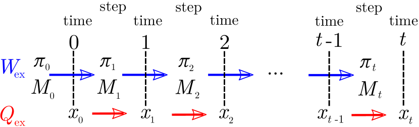
Figure 1: Excess Heat and excess work definition in a discrete time Markov Chain. $x_{n}$ are the state of the system at time $n$. $M_{n}$ are the transition matrices at the $n$th time step and $\pi_{n}$ are the corresponding unique invariant distribution.

The fluctuating relative entropy between $P_{n}$ and $\pi_{n}$ is given by

$$F_{n}(x)=\Phi_{n}(x)-S_{n}(x)=\ln\frac{P_{n}(x)}{\pi_{n}(x)}.$$ (52)

For systems with detailed balance, the sum of this fluctuating relative entropy and the free energy defined in classical equilibrium thermodynamics was called nonequilibrium free energy in Parrondo et al. (2015). For this reason, the relative entropy also got a name nonsteady-state addition (to free energy) in Riechers and Crutchfield (2017). Furthermore, it was shown in Qian (2001c) that this relative entropy itself could be understood physically as a “free energy” as well. To avoid possible confusion on the terminology in this paper, we would follow Altaner (2017) and call this (fluctuating) exergy from now on.. For a trajectory $\omega=x_{0:t}$, the exergy that got absorbed by the system is then

$$\Delta F(x_{0:t})=\ln\frac{P_{t}(x_{t})}{\pi_{t}(x_{t})}-\ln\frac{P_{0}(x_{0})}{\pi_{0}(x_{0})}.$$ (53)

The difference between the exergy dissipation $-\Delta F$ and the excess work done by the system $W_{\mathrm{ex}}$ then gives us the non-adiabatic EP, $S_{\mathrm{na}}$, defined in (Esposito and Van den Broeck, 2010),

$$S_{\mathrm{na}}(\omega) =-\Delta F(\omega)-W_{\mathrm{ex}}(\omega)$$ (54a)

$$=Q_{\mathrm{ex}}(\omega)+\Delta S(\omega)$$ (54b)

$$=\ln\frac{\mathrm{d}\mathbb{P}\ \ \ \ \thinspace}{\mathrm{d}\mathbb{P}^{\mathrm{R}\dagger\mathrm{T}}}(\omega).$$ (54c)

The equivalence between the last two lines can be seen by a direct computation of $P_{0:t}^{\mathrm{R}\dagger\mathrm{T}}(x_{0:t})$. We note that $S_{\mathrm{na}}$ becomes the exergy dissipation $-\Delta F$ in time homogeneous processes since $W_{\mathrm{ex}}=0$ in time homogeneous processes. We also note that the non-adiabatic EP is also additive when connecting time interval,

$$S_{\mathrm{na}}(x_{0:t})=S_{\mathrm{na}}(x_{0:s})+S_{\mathrm{na}}(x_{s:t})$$ (55)

which is obvious from its relation to $W_{\mathrm{ex}}$ and $\Delta F$. Note that $S_{\mathrm{na}}$ reduces to the dissipative work $W_{\mathrm{d}}$ defined in (Jarzynski, 1997; Crooks, 1998) for systems with detailed balance.

Similar to the total EP $S_{\mathrm{tot}}$, the non-adiabatic EP $S_{\mathrm{na}}$ admit neither the TFT nor the odd-parity, sufficient condition for iDFT since the composite operator $\mathrm{R\dagger T}$ is not involutive in general. For rDFT, we compute

$$\bar{S}_{\mathrm{na}}(r(\omega)) =\ln\frac{\mathrm{d}\mathbb{P}^{\mathrm{RT}}\ }{\mathrm{d}\mathbb{P}^{\mathrm{RR}\dagger}}(\omega)$$ (56a)

$$=\ln\frac{P_{t}(X_{t})}{P_{t}^{\mathrm{R}}(X_{0})}\prod_{n=1}^{t}\frac{M_{n}(X_{n-1}|X_{n})}{M_{n}^{\dagger}(X_{n}|X_{n-1})}$$ (56b)

where the denominator can be obtained by using Equation (32) for $\mathbb{P}^{\mathrm{RR}}$ and apply $\dagger$ on it. Now, since

$$\frac{M_{n}(X_{n-1}|X_{n})}{M_{n}^{\dagger}(X_{n}|X_{n-1})}=\frac{\pi_{n}(X_{n-1})}{\pi_{n}(X_{n})},$$ (57)

we get

$$\bar{S}_{\mathrm{na}}(r(\omega))=\ln\frac{P_{0}(X_{0})}{P_{t}^{\mathrm{R}}(X_{0})}-S_{\mathrm{na}}(\omega).$$ (58)

We see that the condition for the odd parity to hold, $\bar{S}_{\mathrm{na}}(r(\omega))=-S_{\mathrm{na}}(\omega)$, is $P_{0}=P_{t}^{\mathrm{R}},$ i.e., $\mathrm{R}$ to be involutive! Hence, similar to the total EP $S_{\mathrm{tot}}$, the non-adiabatic EP $S_{\mathrm{na}}$ admits rDFT if the CPM operator $\mathrm{R}$ is involutive. The rDFT of $S_{\mathrm{na}}$ is an extension to Crooks’ fluctuation theorem (Crooks, 1998, 1999, 2000).

IV.6 Martingale Properties of Entropy Productions

With our measure-theoretic understanding of EPs, more statistical properties of EPs could be found by revealing more on the mathematical properties of their corresponding RNDs and CPM operators. For example, by recognizing the RND of $Q_{\mathrm{hk}}$, $\exp(-Q_{\mathrm{hk}})$, is a martingale, a statistics of the infimum of $Q_{\mathrm{hk}}$ is introduced in Chétrite and Gupta (2011); Neri et al. (2017); Chétrite et al. (2019). Here, we shall discuss the martingale properties of the four EPs and the conditions for the exponential of the negative of them to be a martingale.

In our discrete time Markov chain paradigm, a functional $M(X_{0:t})$ is a martingale if it satisfies

$$\mathbb{E}[M(X_{0:t})|X_{0:s}]=M(X_{0:s})$$ (59)

$\forall s\in\left\{0,1,\cdots,t\right\}$. It can be shown rather straightforwardly that since $S_{\mathrm{T}}$ is not additive in time, $\exp(-S_{\mathrm{T}})$ would not generally be a martingale. Thus, in the following discussion, we will focus on $S_{\mathrm{tot}}$, $Q_{\mathrm{hk}}$, and $S_{\mathrm{na}}$.

We note that all of $S_{\mathrm{tot}}$, $Q_{\mathrm{hk}}$, and $S_{\mathrm{na}}$ are additive in time. Therefore, for $\exp(-S_{\nu})$ to be a martingale where $\nu=\mathrm{RT},\dagger,$or $\mathrm{R\dagger\mathrm{T}}$, we need

$$\mathbb{E}[e^{-S_{\nu}(X_{0:t})}|X_{0:s}] =e^{-S_{\nu}(X_{0:s})}\mathbb{E}[e^{-S_{\nu}(X_{s:t})}|X_{0:s}]$$ (60a)

$$=e^{-S_{\nu}(X_{0:s})}\mathbb{E}[e^{-S_{\nu}(X_{s:t})}|X_{s}]$$ (60b)

$$\stackrel{{\scriptstyle!}}{{=}}e^{-S_{\nu}(X_{0:s})}.$$ (60c)

We thus want to have

$$\mathbb{E}[e^{-S_{\nu}(X_{s:t})}|X_{s}]=1,$$ (61)

$\forall s\in\left\{0,1,\cdots,t\right\}$.

By using the definition for $\nu=\mathrm{RT},\dagger$, and $\mathrm{R}\dagger\mathrm{T}$, one will find

$$\mathbb{E}[e^{-S_{\mathrm{tot}}(X_{s:t})}|X_{s}] =\frac{P_{\mathrm{end}}^{\mathrm{R}}(X_{s})}{P_{s}(X_{s})},$$ (62a)

$$\mathbb{E}[e^{-Q_{\mathrm{hk}}(X_{s:t})}|X_{s}] =1,\text{ and }$$ (62b)

$$\mathbb{E}[e^{-S_{\mathrm{na}}(X_{s:t})}|X_{s}] =\frac{P_{\mathrm{end}}^{\mathrm{R}\dagger}(X_{s})}{P_{s}(X_{s})}$$ (62c)

where

$$P_{\mathrm{end}}^{\mathrm{R}}(x_{s}) =\sum_{x_{s+1:t}}P_{t}(x_{t})\prod_{n=0}^{t-s-1}M_{t-n}(x_{t-n-1}|x_{t-n})\text{ and }$$

$$P_{\mathrm{end}}^{\mathrm{R\dagger}}(x_{s}) =\sum_{x_{s+1:t}}P_{t}(x_{t})\prod_{n=0}^{t-s-1}M_{t-n}^{\dagger}(x_{t-n-1}|x_{t-n})$$ (63)

are the terminal distributions of the processes $\mathrm{R}$ and $\mathrm{R}\dagger$ defined on the time interval $s:t$.

This shows that $\exp(-Q_{\mathrm{hk}})$ is always a martingale which implies that $Q_{\mathrm{hk}}$ is a submartingale satisfying

$$\mathbb{E}[Q_{\mathrm{hk}}(X_{0:t})|X_{0:s}]\geq Q_{\mathrm{hk}}(X_{0:s})$$ (64)

by the convexity of negative logarithm. Since $s$ is arbitrary in $0:t$, the RHS of Equation (62a) and (62c) needs to be 1 for all $x_{s}$ and $s$. This means that $\exp(-S_{\mathrm{tot}})$ or $\exp(-S_{\mathrm{na}})$ are only martingale when the reversal $\mathrm{R}$ or $\mathrm{R\dagger}$ recovers all the marginal distributions in a reversed order: $P_{t}\rightarrow P_{t-1}\rightarrow\cdots\rightarrow P_{0}$ in the reversed process, which is not generally true. One exception is when the dynamics is time homogeneous and also starts with the invariant distribution such that $P_{n}=\pi$, $\forall n\in\left\{0,1,\cdots,t\right\}$.

IV.7 Summary

The properties of the four EPs in physics and chemistry including various FRs we have discussed above have been summarized in Table 2. Here, we note that the three reversals $\mathrm{T}$, $\mathrm{R}$, and $\dagger$ are actually related. By direct computation, one can get

$$\frac{\mathrm{d}\mathbb{P}\ \ \ }{\mathrm{d}\mathbb{P}^{\mathrm{RT}}}=\frac{\mathrm{d}\mathbb{P}\ }{\mathrm{d}\mathbb{P}^{\dagger}}\frac{\mathrm{d}\mathbb{P}\ \ \ \ \thinspace}{\mathrm{d}\mathbb{P}^{\mathrm{R}\dagger\mathrm{T}}}$$ (65)

which leads to the famous decomposition of the total EP introduced in (Ge, 2009),

$$S_{\mathrm{tot}}=S_{\mathrm{na}}+Q_{\mathrm{hk}}.$$ (66)

Since $Q_{\mathrm{hk}}=0$ when the system possesses detailed balance, we also see that $S_{\mathrm{tot}}\equiv S_{\mathrm{na}}$ in detailed balance systems.

IV.8 Two Fluctuation Relations for Heat and Work

As an another demonstration on how the formalism can help us obtain statistical properties of EP-related quantities, we note that there is another generally valid FR called differential fluctuation theorem for the work done by the system $W$, derived in (Jarzynski, 2000; Maragakis et al., 2008) and experimental verified in (Hoang et al., 2018) for detailed balanced systems. Here we provide a more general derivation to extend it to non-detailed balanced systems. The key observation is that the excess work defined in Equation (51b) always has odd parity under the composite CPM operator $\mathrm{C}\equiv\mathrm{RT}$, i.e. $\bar{W}_{\mathrm{ex}}(r(\omega))=-W_{\mathrm{ex}}(\omega)$. Knowing this, we can consider the joint probability of the work $W_{\mathrm{ex}}$, initial state $X_{0}$, and the terminal state $X_{t}$,

$$P_{W_{\mathrm{ex}},X_{0},X_{t}}(w,x_{0},x_{t}) =\mathbb{E}[\mathbb{I}_{\{W_{\mathrm{ex}}\in\mathrm{d}w,X_{0}=x_{0},X_{t}=x_{t}\}}].$$ (67)

The joint probability under the measure $\mathbb{P}^{\mathrm{R}\dagger\mathrm{T}}$ is then given by

$$P_{W_{\mathrm{ex}},X_{0},X_{t}}^{\mathrm{R}\dagger\mathrm{T}}(w,x_{0},x_{t})$$

$$=\mathbb{E}[e^{-S_{\mathrm{na}}}\mathbb{I}_{\{W_{\mathrm{ex}}\in\mathrm{d}w,X_{0}=x_{0},X_{t}=x_{t}\}}]$$ (68a)

$$=e^{w+\Delta F(x_{0},x_{t})}\mathbb{E}[\mathbb{I}_{\{W_{\mathrm{ex}}\in\mathrm{d}w,X_{0}=x_{0},X_{t}=x_{t}\}}]$$ (68b)

$$=e^{w+\Delta F(x_{0},x_{t})}P_{W_{\mathrm{ex}},X_{0},X_{t}}(w,x_{0},x_{t})$$ (68c)

where we have used the fact that the exergy increment $\Delta F(\omega)=\ln\frac{P_{t}(X_{t})}{\pi_{t}(X_{t})}-\ln\frac{P_{0}(X_{0})}{\pi_{0}(X_{0})}$ is a function of $X_{0}$ and $X_{t}$.

By using $\bar{W}_{\mathrm{ex}}(r(\omega))=-W_{\mathrm{ex}}(\omega)$, we thus have

$$\frac{P_{W_{\mathrm{ex}},X_{0},X_{t}}(w,x_{0},x_{t})}{P_{\bar{W}_{\mathrm{ex}},X_{0}^{\mathrm{T}},X_{t}^{\mathrm{T}}}^{\mathrm{R}\dagger}(-w,x_{t},x_{0})}=e^{-\Delta F(x_{0},x_{t})-w}.$$ (69)

Also, a similar differential fluctuation theorem for the excess heat dissipated $Q_{\mathrm{ex}}(\omega)$ can also be derived,

$$\frac{P_{Q_{\mathrm{ex}},X_{0},X_{t}}(q,x_{0},x_{t})}{P_{\bar{Q}_{\mathrm{ex}},X_{0}^{\mathrm{T}},X_{t}^{\mathrm{T}}}^{\mathrm{R}\dagger}(-q,x_{t},x_{0})}=e^{q+\Delta S(x_{0},x_{t})}$$ (70)

since $\bar{Q}_{\mathrm{ex}}(r(\omega))=-Q_{\mathrm{ex}}(\omega)$ and $S_{\mathrm{na}}=-\Delta F-W_{\mathrm{ex}}=Q_{\mathrm{ex}}+\Delta S$.

V Entropy Productions in Constant-noise Diffusion Processes

We will now briefly go through how to use measure-theoretic probability theory and the CPM operator formalism to derive the stochastic integral formulas for the four EPs in time inhomogeneous constant-noise diffusion processes. With the formulas, one can further derive the expression for the moments of EPs with Ito calculus. In a constant-noise diffusion process in $\mathbb{R}^{n}$, the probability density of the microstate variable $\mathbf{X}_{t}$, $p(\mathbf{x},t)$, is governed by the Fokker-Planck Equation,

$$\frac{\partial}{\partial t}p(\mathbf{x},t)=-\nabla\cdot\mathbf{J}[p(\mathbf{x},t)]$$ (71)

with probability flux given by

$$\mathbf{J}[p(\mathbf{x},t)]=\mathbf{b}(\mathbf{x},t)p(\mathbf{x},t)-\mathbf{D}\nabla p(\mathbf{x},t).$$ (72)

and the stochastic trajectory governed by the stochastic differential equation,

$$\mathrm{d}\mathbf{X}_{t}=\mathbf{b}(\mathbf{X}_{t},t)\mathrm{d}t+\mathbf{\Gamma}\mathrm{d}\mathbf{W}_{t},$$ (73)

where $\mathbf{D}=\mathbf{\Gamma}\mathbf{\Gamma}^{\mathsf{T}}/2$ is a constant diffusion matrix ($\mathsf{T}$ denoting transpose) and $\mathbf{W}_{t}$ is the $n$ dimensional Wiener processes (Brownian motions) with each component independent and having unit strength of noise.

To derive the stochastic integral formula for the four EPs from their RND definitions, we rely on Girsanov theorem Jiang et al. (2004) to give us the RND to “kill” the drift $\mathbf{b}(\mathbf{X}_{t},t)$ in the dynamics of $\mathbf{X}_{t}$. Given a time interval $t\in\left[0,\tau\right]$ and the RND

$$\frac{\mathrm{d}\mathbb{P}^{\mathrm{B}}}{\mathrm{d}\mathbb{P}_{\ \thinspace}} =e^{-\frac{1}{2}\int_{0}^{\tau}\mathbf{D}^{-1}\mathbf{b}\cdot\mathrm{d}\mathbf{X}_{t}+\frac{1}{4}\int_{0}^{\tau}\mathbf{b}\cdot\mathbf{D}^{-1}\mathbf{b}\mathrm{d}t}$$ (74a)

$$=e^{-\frac{1}{2}\int_{0}^{\tau}\mathbf{D}^{-1}\mathbf{b}\circ\mathrm{d}\mathbf{X}_{t}+\frac{1}{2}\int_{0}^{\tau}\nabla\cdot\mathbf{b}\mathrm{d}t+\frac{1}{4}\int_{0}^{\tau}\mathbf{b}\cdot\mathbf{D}^{-1}\mathbf{b}\mathrm{d}t},$$ (74b)

the probability density of the process $\mathbf{X}_{t}$ under the measure $\mathbb{P}^{\mathrm{B}}$ satisfies $\frac{\partial}{\partial t}p^{\mathrm{B}}(\mathbf{x},t)=\nabla\cdot\mathbf{D}\nabla p^{\mathrm{B}}(\mathbf{x},t)$, i.e. $\mathbf{X}_{t}$ is a Brownian motion with strength $\mathbf{\Gamma}$ under $\mathbb{P}^{\mathrm{B}}$. The CPM operator B “kills” the drift by changing of the probability measure from $\mathbb{P}$ to $\mathbb{P}^{\mathrm{B}}$. We note that the first stochastic integral in Equation (74a) is an Ito integral and the first stochastic integral in Equation (74b) is a Stratonovich integral. We rewrote the stochastic integral into a Stratonovich form for later convenience when considering time reversals.

V.1 Dissipation Function

To use Equation (74b) to get $S_{\mathrm{T}}$, we perform the decomposition of its corresponding RND,

$$\frac{\mathrm{d}\mathbb{P}\ \thinspace}{\mathrm{d}\mathbb{P}^{\mathrm{T}}}=\frac{\mathrm{d}\mathbb{P}\ \ }{\mathrm{d}\mathbb{P}^{\mathrm{B}}}\frac{\mathrm{d}\mathbb{P}^{\mathrm{B}}\ \thinspace}{\mathrm{d}\mathbb{P}^{\mathrm{BT}}}\frac{\mathrm{d}\mathbb{P}^{\mathrm{BT}}}{\mathrm{d}\mathbb{P}^{\mathrm{T}}\ \thinspace}.$$ (75)

We already have the first term $\frac{\mathrm{d}\mathbb{P}\ \ }{\mathrm{d}\mathbb{P}^{\mathrm{B}}}=-\frac{\mathrm{d}\mathbb{P}^{\mathrm{B}}}{\mathrm{d}\mathbb{P}_{\ \thinspace}}$ by Equation (74b). For the third term, it can be rewritten as

$$\frac{\mathrm{d}\mathbb{P}^{\mathrm{B}}}{\mathrm{d}\mathbb{P}_{\ \thinspace}}(r(\omega))= \exp\{\frac{1}{2}\int_{0}^{\tau}\mathbf{D}^{-1}\mathbf{b}(\mathbf{X}_{t},\tau-t)\circ\mathrm{d}\mathbf{X}_{t}$$

$$+\frac{1}{2}\int_{0}^{\tau}\nabla\cdot\mathbf{b}(\mathbf{X}_{t},\tau-t)\mathrm{d}t$$

$$+\frac{1}{4}\int_{0}^{\tau}\mathbf{b}\cdot\mathbf{D}^{-1}\mathbf{b}(\mathbf{X}_{t},\tau-t)\mathrm{d}t\}$$ (76)

where I have used the change of integration variable for the three integrals in the exponent using

$$\int_{0}^{\tau}\mathbf{b}(\mathbf{X}_{\tau-t},t)\circ\mathrm{d}\mathbf{X}_{\tau-t} =-\int_{0}^{\tau}\mathbf{b}(\mathbf{X}_{t},\tau-t)\circ\mathrm{d}\mathbf{X}_{t}\text{ and }$$

$$\int_{0}^{\tau}f(\mathbf{X}_{\tau-t},t)\mathrm{d}t =\int_{0}^{\tau}f(\mathbf{X}_{t},\tau-t)\mathrm{d}t.$$ (77)

We note that the first equality in Equation (77) is true since it is a Stratonovich integral. If the stochastic integral is in any other integration scheme, the change of integration variable will lead to a change of integral scheme.

The second term in Equation (75) is the RND of the dissipation function in Brownian motion. Since $\mathbf{X}_{t}$ is drift-free under $\mathbb{P}^{\mathrm{B}}$ and the noise strength is a constant, the conditional probability for having a path $\omega=x_{0:t}$ conditioning that it starts at $x_{0}$ is the same as the one for the reversed path $r(\omega)=x_{t:0}$ conditioning that it starts at $x_{t}$ due to the symmetry of Brownian motion. We thus see that the $\mathrm{T}$ operator only changes $\mathbb{P}^{\mathrm{B}}$ by the initial probability density $p_{0}$ from evaluating at $\mathbf{X}_{0}$, $p_{0}(\mathbf{X}_{0})$, to evaluating at $\mathbf{X}_{\tau}$, $p_{0}(\mathbf{X}_{\tau})$, and the change of measure is completed by

$$\frac{\mathrm{d}\mathbb{P}^{\mathrm{B}}\ \thinspace}{\mathrm{d}\mathbb{P}^{\mathrm{BT}}}=\frac{p_{0}(\mathbf{X}_{0})}{p_{0}(\mathbf{X}_{\tau})}$$ (78)

where I have also used that the operator B leaves the initial probability density invariant, $p_{0}^{\mathrm{B}}=p_{0}$.

Putting Equation (75-78) together, we arrive the dissipation function for a time inhomogeneous constant-noise diffusion:

$$S_{\mathrm{T}}= \ln\frac{p_{0}(\mathbf{X}_{0})}{p_{0}(\mathbf{X}_{\tau})}+\int_{0}^{\tau}\mathbf{D}^{-1}\bar{\mathbf{b}}\circ\mathrm{d}\mathbf{X}_{t}$$

$$+\frac{1}{2}\int_{0}^{\tau}\delta\left(\nabla\cdot\mathbf{b}\right)\mathrm{d}t+\frac{1}{4}\int_{0}^{\tau}\delta\left(\mathbf{b}\cdot\mathbf{D}^{-1}\mathbf{b}\right)\mathrm{d}t$$ (79)

where we have used the notation

$$\bar{\mathbf{b}}(\mathbf{X}_{t},t) =\left[\mathbf{b}(\mathbf{X}_{t},t)+\mathbf{b}(\mathbf{X}_{t},\tau-t)\right]/2,\text{ and}$$ (80a)

$$\delta f(\mathbf{X}_{t},t) =f(\mathbf{X}_{t},\tau-t)-f(\mathbf{X}_{t},t).$$ (80b)

The stochastic integral expression of the dissipation function $S_{\mathrm{T}}$ in Equation (79) in general time inhomogeneous constant-noise diffusion process, as far as we know, is a new result.

We note that if the drift is symmetric in the interval $t\in\left[0,\tau\right]$, i.e. $\mathbf{b}(\cdot,t)=\mathbf{b}(\cdot,\tau-t)$, then the two terms with $\delta$ become zero. The expression for dissipation function then reduces to

$$S_{\mathrm{T}}=\ln\frac{p_{0}(\mathbf{X}_{0})}{p_{0}(\mathbf{X}_{\tau})}+Q$$ (81)

where $Q=\int_{0}^{\tau}\mathbf{D}^{-1}\mathbf{b}\circ\mathrm{d}\mathbf{X}_{t}$ is the heat dissipation. As time homogeneous process being symmetric in the interval, this is consistent with Seifert (2012). It can also be seen from this expression that, consistent with our understanding in our Markov chain paradigm, $S_{\mathrm{T}}$ is not generally additive when connecting time intervals.

V.2 Total Entropy Production

With $S_{\mathrm{tot}}=\ln\frac{\mathrm{d}\mathbb{P}\ \ \ }{\mathrm{d}\mathbb{P}^{\mathrm{RT}}}$, we derive the formula of it in a similar decomposition of the corresponding RND,

$$\frac{\mathrm{d}\mathbb{P}\ \ \ }{\mathrm{d}\mathbb{P}^{\mathrm{RT}}}(\omega)=\frac{\mathrm{d}\mathbb{P}\ \ }{\mathrm{d}\mathbb{P}^{\mathrm{B}}}\frac{\mathrm{d}\mathbb{P}^{\mathrm{B}}\ \ \ }{\mathrm{d}\mathbb{P}^{\mathrm{BRT}}}\frac{\mathrm{d}\mathbb{P}^{\mathrm{BRT}}}{\mathrm{d}\mathbb{P}^{\mathrm{RBT}}}\frac{\mathrm{d}\mathbb{P}^{\mathrm{RBT}}}{\mathrm{d}\mathbb{P}^{\mathrm{RT}}\ \thinspace}.$$ (82)

We can find the second and the fourth RNDs in a similar way. One has

$$\frac{\mathrm{d}\mathbb{P}^{\mathrm{B}}\ \ \ }{\mathrm{d}\mathbb{P}^{\mathrm{BRT}}} =\frac{p_{0}(\mathbf{X}_{0})}{p_{\tau}(\mathbf{X}_{\tau})}$$ (83)

since $\mathrm{RT}$ only changes the initial distribution for $\mathbb{P}^{\mathrm{B}}$ and

$$\frac{\mathrm{d}\mathbb{P}^{\mathrm{RBT}}}{\mathrm{d}\mathbb{P}^{\mathrm{RT}}\ \thinspace}(\omega)= \exp\{\frac{1}{2}\int_{0}^{\tau}\mathbf{D}^{-1}\mathbf{b}(\mathbf{X}_{t},t)\circ\mathrm{d}\mathbf{X}_{t}$$

$$+\frac{1}{2}\int_{0}^{\tau}\nabla\cdot\mathbf{b}(\mathbf{X}_{t},t)\mathrm{d}t$$

$$+\frac{1}{4}\int_{0}^{\tau}\mathbf{b}\cdot\mathbf{D}^{-1}\mathbf{b}(\mathbf{X}_{t},t)\mathrm{d}t\}.$$ (84)

by replacing $\mathbf{b}(\cdot,t)$ with $\mathbf{b}^{\mathrm{R}}(\cdot,t)=\mathbf{b}(\cdot,\tau-t)$ in Equation (76).

Now, for the third term in Equation (82), since B kills the drift for both $\mathbf{b}$ and $\mathbf{b}^{\mathrm{R}}$, the effect of R after composed with B, regardless of the order, is just a change in the initial distribution. BR is thus the same as RB since B doesn’t change the initial distribution. This means the operator B commutes with R, and thus the third term actually equals to one! Putting these together, we can get the famous entropy change decomposition in time inhomogeneous constant-noise diffusion processes,

$$S_{\mathrm{tot}}=\ln\frac{p_{0}(\mathbf{X}_{0})}{p_{\tau}(\mathbf{X}_{\tau})}+Q=\Delta S+Q.$$ (85)

With this, it is obvious that $S_{\mathrm{tot}}$ is additive in time.

We also note that the difference between $S_{\mathrm{T}}$ and $S_{\mathrm{tot}}$ in processes with time symmetric $\mathbf{b}$, i.e. when $\mathbf{b}^{\mathrm{R}}=\mathbf{b}$, is

$$S_{\mathrm{T}}-S_{\mathrm{tot}}=\ln\frac{p_{\tau}(\mathbf{X}_{\tau})}{p_{0}(\mathbf{X}_{\tau})}.$$ (86)

This is consistent with what we had in Equation (40c), leading one to conclude $\mathbb{E}[S_{\mathrm{T}}]\geq\mathbb{E}[S_{\mathrm{tot}}]$ when $\mathbf{b}^{\mathrm{R}}=\mathbf{b}$.

V.3 Housekeeping heat and Non-adiabatic Entropy Production

Using the CPM perspective to get $Q_{\mathrm{hk}}$ has already been rigorously studied in Jiang et al. (2004), here we shall briefly revisit the derivation and rely on the relation $S_{\mathrm{tot}}=Q_{\mathrm{hk}}+S_{\mathrm{na}}$ to get the formula for $S_{\mathrm{na}}$.

In time inhomogeneous diffusion process, we could consider the instantaneous stationary probability density $\pi_{t}$ such that

$$\nabla\cdot\mathbf{J}[\pi_{t}]=0$$ (87)

where $\mathbf{J}[\pi_{t}]=\mathbf{b}(\mathbf{X}_{t},t)\pi_{t}-\mathbf{D}\nabla\pi_{t}$. From the fact that the adjoint process is given by reversing $\mathbf{J}[\pi_{t}]$, we see that the effect of the operator $\dagger$ on $\mathbf{b}$ is given by

$$\mathbf{b}^{\dagger}=-\mathbf{b}-2\mathbf{D}\nabla\left(-\ln\pi_{t}\right).$$ (88)

Then, we use the decomposition

$$\frac{\mathrm{d}\mathbb{P}\ }{\mathrm{d}\mathbb{P}^{\dagger}}=\frac{\mathrm{d}\mathbb{P}\ \ }{\mathrm{d}\mathbb{P}^{\mathrm{B}}}\frac{\mathrm{d}\mathbb{P}^{\mathrm{B}}\ }{\mathrm{d}\mathbb{P}^{\dagger\mathrm{B}}}\frac{\mathrm{d}\mathbb{P}^{\dagger\mathrm{B}}}{\mathrm{d}\mathbb{P}^{\dagger}\ }$$ (89)

and note that the second term is 1 since neither $\dagger$ nor B changes the initial distribution and B kills the drift no matter it is $\mathbf{b}$ or $\mathbf{b}^{\dagger}$. Also, the third term can be evaluated by Equation (74b) by substituting $\mathbf{b}$ with $\mathbf{b}^{\dagger}$. Further using Equation (87) to simplify the expression one got from above, one would arrive

$$Q_{\mathrm{hk}} =\int_{0}^{\tau}\left[\mathbf{D}^{-1}\mathbf{b}+\nabla\left(-\ln\pi_{t}\right)\right]\circ\mathrm{d}\mathbf{X}_{t}$$

$$=Q-Q_{\mathrm{ex}}$$ (90)

where $Q_{\mathrm{ex}}=-\int_{0}^{\tau}\nabla\left(-\ln\pi_{t}\right)\circ\mathrm{d}\mathbf{X}_{t}$ is the excess heat dissipation in diffusion. The non-adiabatic entropy production $S_{\mathrm{na}}$ would then be given by

$$S_{\mathrm{na}} =S_{\mathrm{tot}}-Q_{\mathrm{hk}}=W_{\mathrm{ex}}-\Delta F$$

$$=\int_{0}^{\tau}\frac{\partial\left(-\ln\pi_{t}\right)}{\partial t}\mathrm{d}t-\ln\frac{p_{\tau}(X_{\tau})\pi_{0}(X_{0})}{\pi_{\tau}(X_{\tau})p_{0}(X_{0})}.$$ (91)

VI Discussion

In this paper, we characterize the difference between the statistical properties of the original stochastic process and the one after reversal by a change of probability measure, an analog to Schrödinger’s picture on Quantum Mechanics (Qian et al., 2019). A change in statistical properties from a physical operation is represented by an operator $\nu$ operating on a probability measure $\mathbb{P}$ in the probability measure space $\mathcal{P}$. With our mathematically more general and concise CPM formalism, we have presented a comprehensive study of the properties of EPs including FRs. Sufficient conditions for the FRs of the four EPs are summarized in Table 2. Importantly, a hierarchy of the generality for FRs in general stochastic processes can be revealed from our work: both IFT and GFR are generally true; rDFT and iDFT require odd parity symmetry with different $\hat{S}_{\nu}$ as stated in (Seifert, 2012); and TFT further requires the CPM operator to be realized by an involutive map on the trajectory space $\Omega$. This hierarchical structure of the domain of validity for FRs reveals relation between FRs such as TFT implies iDFT.

We further demonstrate how to obtain other properties of EPs from their logarithm RND definitions such as their martingale properties and distinguish the difference between dissipation function introduced by Evans and Searles Evans and Searles (2002) and the total entropy production. The “paradox” that the two EPs have the same entropy production rate but with non-negative difference in expectation for finite time interval in time homogeneous processes is resolved by noting the failure of time additivity for the dissipation function. Stochastic integration expressions for the two EPs are also derived in general time inhomogeneous constant-noise diffusion to better see the contradistinction of their physical meaning and properties.

It is important to note that throughout this paper, we have assumed the state variables $X_{n}$ to have even parity under the time reversal, i.e. they are position-like physical quantities. One extension to our work is to consider variables that have odd parity under time reversal such as velocity (Spinney and Ford, 2012; Ge, 2014; Li and Tu, 2019).

The unit of EP $S_{\nu}$ is chosen to be in the natural unit of information (nat) throughout the paper (Crooks, 1999; Cover and Thomas, 2006). And temperature of the heat reservoir is assumed to be constant. When considering diffusion processes in Section V, we have also restricted ourselves to constant-noise diffusion processes. If the strength of noise $\mathbf{\Gamma}$ varies in spacetime, then the use of Girsanov theorem to derive the formula for $S_{\mathrm{T}}$ and $S_{\mathrm{tot}}$ becomes more involved since $\frac{\mathrm{d}\mathbb{P}_{0}}{\mathrm{d}\mathbb{P}_{0}^{\nu}}$ where $\nu=\mathrm{T}$ or $\mathrm{RT}$ becomes less straightforward. We note that Jiang, Qian, and Qian have used Girsanov theorem to derive the housekeeping heat $Q_{\mathrm{hk}}$ for autonomous, non-constant noise diffusion in Jiang et al. (2004). With this and replying on the fact that the formula of $S_{\mathrm{na}}$ does not depend on $\mathbf{\Gamma}$, we can use the relation $S_{\mathrm{tot}}=Q_{\mathrm{hk}}+S_{\mathrm{na}}$ to argue that Equation (85) still holds for autonomous, non-constant noise diffusion processes. To obtain the integral equation for $S_{\mathrm{T}}$, however, will need other methods. One may need the path integral formalism to obtain the probability “density” of a diffusion path Onsager and Machlup (1953), or make use of the Riemann geometry introduced by $\mathbf{\Gamma}$ and $\mathbf{D}$ to consider a constant-noise diffusion on a curved space Fujita and Kotani (1982).

The general theory we presented in Section II is in fact a general result for fluctuating relative entropy and its statistical properties. It can also be applied to entropies defined in information theory (Cover and Thomas, 2006). For example, suppose we have a finite state space $\mathcal{X}\equiv\Omega$, i.e. there is a fundamental state random variable $X$ that labels every $\omega\in\Omega$ with a unique real number, we can then choose $P_{X}^{\nu}$ to be the uniform distribution, i.e. $\mathbb{P}^{\nu}$ as the Lebesgue measure, to get an entropy corresponding to the maximum entropy $\ln\|\Omega\|$ minuses the fluctuating Shannon entropy of the system,

$$H(\omega)=\ln\|\Omega\|-\left[-\ln P_{X}(X(\omega))\right]$$ (92)

where $\|\Omega\|$ represents the size of the sample space. Another example would be to have $\Omega=\mathcal{X}\otimes\mathcal{Y}$ and consider the fluctuating mutual information between two random variables $X$ and $Y$,

$$I(\omega)=\ln\frac{P_{X,Y}(X(\omega),Y(\omega))}{P_{X}(X(\omega))P_{Y}(Y(\omega))}.$$ (93)

Our theory immediately implies that both $H(\omega)$ and $I(\omega)$ have non-negative expectation, and admit IFT and GFR.

The combination of information theory and stochastic thermodynamics is a natural application and extension to the theory (Landauer, 1961; Bennett, 1982; Still et al., 2012; Parrondo et al., 2015). One example would be to consider random transition matrices for stochastic driving protocol. With randomness in transition matrices, the second law of thermodynamics is refined by incorporating the mutual information between the past and present, and the mutual information between the present and the future, giving us a thermodynamics of prediction (Still et al., 2012). In our change-of-measure formalism, we could extend $\left(\Omega,\mathcal{F}\right)$ to include all possible transition matrices. Such future work could be conducted by considering the theories of random dynamical system for Markov chains (Ye et al., 2016; X. F. Ye and Qian, 2019).

Appendix

A. Modern Probability Theory and Radon-Nikodym Derivative

Here we briefly introduce several key concepts of modern measure-theoretic probability theory pioneered by A. N. Kolmogorov (Kolmogorov, 2018). For recent textbook introductions, see (Durrett, 2010; Grimmett and Stirzaker, 2001). One of the most important concept in the theory is that one specifies the sample space $\Omega$, the $\sigma$-algebra $\mathcal{F},$ and a probability (measure) $\mathbb{P}$ to start any probabilistic discussion on stochastic processes.

An outcome $\omega$ is a particular result of a random trial. A sample space $\Omega$ is the collection of all possible outcomes. We can think of $\Omega$ as the state space of our system of interest. In this paper, a “state” of the system of interest would be a trajectory of a given finite time interval $t$ in a stochastic process. $\Omega$ then becomes the space of trajectories.

An event of interest $A$ is a subset of the sample space that we seek the probability of. For example, in this paper, it can be the set of periodic trajectories $\omega\in\Omega$, i.e. we might ask “what is the probability of having a periodic trajectory”. The collection of all event of interests of $\Omega$ is called $\sigma$-algebra , usually denoted as $\mathcal{F}$.

Note that when we are interested in an event, the complement of it, $A^{c}$, i.e. when $A$ does not happen, is also under our interest. Moreover, if we are already interested in a bunch of events $A_{1},A_{2}^{c},\dots$, then the countable union of them, i.e. the event when at least one of it happen, is also interesting to us. Note that with complement and countable union, the countable intersections are automatically included in $\mathcal{F}$.

As a result, a $\sigma$-algebra of $\Omega$ as a collection of all events of interest must have the following three properties in its very definition: (1) containing the empty set $\emptyset$ where nothing happen, (2) being closed under countable union, and (3) being closed under complement. One of the many reasons to introduce $\sigma$-algebra $\mathcal{F}$ along with the sample space $\Omega$ is that since we are interested in knowing the probability of every events of interest, which is given by a probability measure $\mathbb{P}$, we need the collection of all events of interest $\mathcal{F}$ to actually define a $\mathbb{P}$.

A probability measure $\mathbb{P}$ measures the probability of an event of interest $A\in\mathcal{F}$ by assigning the event a real value, $\mathbb{P}\{A\}$, between 0 and 1. Since an event $A\in\mathcal{F}$ is a subset of $\Omega$, the probability of an event $A$ can also be represented as an expectation of the indicator function of an event $A$, $\mathbb{I}_{A}(\omega)$, i.e.

$$\mathbb{P}\{A\}=\mathbb{E}[\mathbb{I}_{A}(\omega)]$$ (A1)

where $\mathbb{I}_{A}(\omega)$ gives $1$ if $\omega\in A$ and $0$ otherwise, and $\mathbb{E}[\cdot]$ denotes the expectation. This expectation expression of $\mathbb{P}\{A\}$ is convenient in many calculations, especially when we consider a change of probability measure as shown in Equation (2b) and (3).

Physical observable as a random variable $X(\omega)$ is not just a function from $\Omega$ to $\mathbb{R}$. Since we are interested in the statistical properties of $X(\omega)$, we would like to use the probability measure $\mathbb{P}$ defined on the $\mathcal{F}$ of $\Omega$ to get the probability of an event such as $\left\{X(\omega)\in(a,b);a,b\in\mathbb{R}\right\}$ or for $X(\omega)$ in any countable union/complements of open intervals. The collection of any set that can be formed from open intervals in $\mathbb{R}$, complement of them, and/or countable union of them is called the Borel sets of $\mathbb{R}$, denoted as $\mathcal{B}(\mathbb{R})$. The requirement of being able to use a probability measure $\mathbb{P}$ to get that statistical properties of $X(\omega)$ is then the requirement of measurability. That is, for $\mathbb{P}\{X(\omega)\in B\}$ to make sense, we need that $\forall B\in\mathcal{B}(\mathbb{R})$, $\left\{X(\omega)\in B\right\}$ as a set of $\omega$ to be in $\mathcal{F}$. Hence, a random variable is not a function of $\Omega$ but a measurable function $X(\omega):\Omega\mapsto\mathbb{R}$ defined on $\left(\Omega,\mathcal{F}\right)$ so that $\left\{X(\omega)\in B\right\}\in\mathcal{F}$, $\forall B\in\mathcal{B}(\mathbb{R})$.

The very fact that $X$ is defined on a pair $\left(\Omega,\mathcal{F}\right)$, without a specific $\mathbb{P}$, is a manifestation of the Schrödinger’s picture of changes in statistical properties. For two different stochastic processes, the change in the statistical properties of a random variable $X(\omega)$, the difference in its distribution $P_{X}$ and $P_{X}^{\nu}$, is due to the change of probability measure $\mathbb{P}\rightarrow\mathbb{P}^{\nu}$ (Qian et al., 2019). Without $\mathbb{P}$, the pair $\left(\Omega,\mathcal{F}\right)$ is called measurable space. With a $\mathbb{P}$ defined, the triple $\left(\Omega,\mathcal{F},\mathbb{P}\right)$ is called the probability space. In this paper, a stochastic process is specified by a probability space.

With a given measurable space $\left(\Omega,\mathcal{F}\right)$, there are many $\mathbb{P}$ that can be considered. Radon-Nikodym derivative (RND) is a special random variable that can be used to change one probability measure $\mathbb{P}$ to another $\mathbb{P}^{\nu}$, denoted as $\frac{\mathrm{d}\mathbb{P}^{\nu}}{\mathrm{d}\mathbb{P}\ }(\omega)$. As explained in the main context, the probability of a event $A\in\mathcal{F}$ in the new probability measure is given by the expectation representation shown in Equation (A1),

$$\mathbb{P}^{\nu}\{A\}=\mathbb{E}^{\nu}[\mathbb{I}_{A}(\omega)]=\mathbb{E}[\frac{\mathrm{d}\mathbb{P}^{\nu}}{\mathrm{d}\mathbb{P}\ }(\omega)\mathbb{I}_{A}(\omega)].$$ (A2)

For $\Omega$ whose $\omega$ in $\Omega$ can be 1-1 labeled by $x\in\mathbb{Z}$, we have the RND reduced to the ratio of probability mass functions $P^{\nu}(x)/P(x)$ since

$$\mathbb{P}^{\nu}\{A\} =\mathbb{E}^{\nu}[\mathbb{I}_{A}]=\sum_{x\in\mathbb{Z}}\mathbb{I}_{A}(x)P^{\nu}(x)$$ (A3a)

$$=\sum_{x\in\mathbb{Z}}\mathbb{I}_{A}(x)\frac{P^{\nu}(x)}{P(x)}P(x)$$ (A3b)

$$=\mathbb{E}[\mathbb{I}_{A}(x)\frac{P^{\nu}(x)}{P(x)}].$$ (A3c)

For those $\Omega$ whose $\omega$ in $\Omega$ can be 1-1 labeled by $x\in\mathbb{R}$ such as diffusion processes, we have the RND reduced to the ratio of probability density functions $\rho^{\nu}(x)/\rho(x)$ since

$$\mathbb{P}^{\nu}\{A\} =\mathbb{E}^{\nu}[\mathbb{I}_{A}]=\int_{\mathbb{R}}\mathbb{I}_{A}(x)\rho^{\nu}(x)\mathrm{d}x$$

$$=\int_{\mathbb{R}}\mathbb{I}_{A}(x)\frac{\rho^{\nu}(x)}{\rho(x)}\rho(x)\mathrm{d}x$$

$$=\mathbb{E}[\mathbb{I}_{A}(x)\frac{\rho^{\nu}(x)}{\rho(x)}].$$ (A4c)

B. Entropy Production Rates for $S_{\mathrm{T}}$ and $S_{\mathrm{tot}}$

With our trajectory-based definitions for dissipation function $S_{\mathrm{T}}$ and total entropy production $S_{\mathrm{tot}}$ given as

$$S_{\mathrm{T}}(\omega)=\ln\frac{\mathrm{d}\mathbb{P}\ \thinspace}{\mathrm{d}\mathbb{P}^{\mathrm{T}}}(\omega)\text{ and }S_{\mathrm{tot}}(\omega)=\ln\frac{\mathrm{d}\mathbb{P}\ \ \ }{\mathrm{d}\mathbb{P}^{\mathrm{RT}}}(\omega)$$ (B1)

where $\omega=x_{0}x_{1}\cdots x_{t}$, here we show that although the two EPs differ in finite time interval as shown in our main context, they have the same rate in expectation in infinitesimal time interval $t\rightarrow 0$.

With an infinitesimal time interval $t\rightarrow 0$, we only need to consider one infinitesimal time step where the system state goes from $i$ to $j$,

$$S_{\mathrm{T}}(i,j)=\ln\frac{P_{0}(i)M(j|i)}{P_{0}(j)M(i|j)}$$ (B2)

and

$$S_{\mathrm{tot}}(i,j)=\ln\frac{P_{0}(i)M(j|i)}{P_{t}(j)M(i|j)}.$$ (B3)

The difference between the two EPs is

$$D(i,j)\coloneqq S_{\mathrm{T}}(i,j)-S_{\mathrm{tot}}(i,j)=\ln\frac{P_{t}(j)}{P_{0}(j)}.$$ (B4)

With $t\rightarrow 0$, $M$ is approaching to an identity matrix,

$$M(j|i)=\delta_{i,j}+q(j|i)\cdot t+O(t^{2}).$$ (B5)

Up to the linear order, we can write

$$P_{t}(j) =\sum_{k}P_{0}(k)M(j|k)$$

$$=P_{0}(j)+t\sum_{k}P_{0}(k)q(j|k)+O(t^{2}).$$ (B6b)

In the literature, entropy production rate of $S_{\mathrm{T}}$ and $S_{\mathrm{tot}}$ is defined as their limiting re-scaled expectation: $\lim_{t\rightarrow 0}\frac{\mathbb{E}[S_{\mathrm{T}}]}{t}$ and $\lim_{t\rightarrow 0}\frac{\mathbb{E}[S_{\mathrm{tot}}]}{t}$. Therefore, let us compute the expectation of $S_{\mathrm{T}}$, $S_{\mathrm{tot}}$, and $D$ as an asymptotic series of small $t$. Since $D=S_{\mathrm{T}}-S_{\mathrm{tot}}$, we have

$$\mathbb{E}[D]=\mathbb{E}[S_{\mathrm{T}}]-\mathbb{E}[S_{\mathrm{tot}}]$$ (B7)

and we will compute $\mathbb{E}[D]$ and $\mathbb{E}[S_{\mathrm{T}}]$.

For $\mathbb{E}[S_{\mathrm{T}}]$, we have

$$\mathbb{E}[S_{\mathrm{T}}] =\sum_{i,j}P_{0}(i)M(j|i)\ln\frac{P_{0}(i)M(j|i)}{P_{0}(j)M(j|i)}$$ (B8a)

$$=0+t\sum_{i,j;i\neq j}P_{0}(i)q(j|i)\ln\frac{P_{0}(i)q(j|i)}{P_{0}(j)q(j|i)}$$ (B8b)

And for $\mathbb{E}[D]$, we have

$$\mathbb{E}[D] =\sum_{i,j}P_{0}(i)M(j|i)\ln\frac{P_{t}(j)}{P_{0}(j)}$$

$$=\sum_{j}P_{t}(j)\ln\frac{P_{t}(j)}{P_{0}(j)}.$$ (B9b)

With $P_{t}(j)=P_{0}(j)+t\sum_{k}P_{0}(k)q(j|k)+O(t^{2})$, we compute

$$\ln\frac{P_{t}(j)}{P_{0}(j)} =\ln\frac{P_{0}(j)+t\sum_{k}P_{0}(k)q(j|k)+O(t^{2})}{P_{0}(j)}$$

$$=t\frac{\sum_{k}P_{0}(k)q(j|k)}{P_{0}(j)}+O(t^{2}).$$ (B10b)

We thus see that

$$\mathbb{E}[D] =t\sum_{j}P_{t}(j)\frac{\sum_{k}P_{0}(k)q(j|k)}{P_{0}(j)}+O(t^{2})$$

$$=t\sum_{k}P_{0}(k)\sum_{j}q(j|k)+O(t^{2})$$

$$=0+O(t^{2}).$$ (B11c)

Hence, the two EPs have the same entropy production rate

$$\mathrm{e_{p}} =\lim_{t\rightarrow 0}\frac{\mathbb{E}[S_{\mathrm{T}}]}{t}$$

$$=\lim_{t\rightarrow 0}\frac{\mathbb{E}[S_{\mathrm{tot}}]+\mathbb{E}[D]}{t}=\lim_{t\rightarrow 0}\frac{\mathbb{E}[S_{\mathrm{tot}}]}{t}.$$ (B12b)

in the infinitesimal time interval limit.

References

- Searles and Evans (1999) D. J. Searles and D. J. Evans, “Fluctuation theorem for stochastic systems,” Phys. Rev. E 60, 159–164 (1999).
- Jiang et al. (2004) D.-Q. Jiang, M. Qian, and M.-P. Qian, Mathematical Theory of Nonequilibrium Steady States: On the Frontier of Probability and Dynamical Systems, 2004th ed. (Springer, Berlin ; New York, 2004).
- Seifert (2012) U. Seifert, “Stochastic thermodynamics, fluctuation theorems and molecular machines,” Rep. Prog. Phys. 75, 126001 (2012).
- Qian (2016) H. Qian, “Nonlinear Stochastic Dynamics of Complex Systems, I: A Chemical Reaction Kinetic Perspective with Mesoscopic Nonequilibrium Thermodynamics,” arXiv:1605.08070 (2016).
- Thompson and Qian (2016) L. F. Thompson and H. Qian, “Nonlinear Stochastic Dynamics of Complex Systems, II: Potential of Entropic Force in Markov Systems with Nonequilibrium Steady State, Generalized Gibbs Function and Criticality,” Entropy 18, 309 (2016).
- Crooks (1998) G. E. Crooks, “Nonequilibrium Measurements of Free Energy Differences for Microscopically Reversible Markovian Systems,” J. Stat. Phys. 90, 1481–1487 (1998).
- Jarzynski (1997) C. Jarzynski, “Nonequilibrium Equality for Free Energy Differences,” Phys. Rev. Lett. 78, 2690–2693 (1997).
- Crooks (1999) G. E. Crooks, “Entropy production fluctuation theorem and the nonequilibrium work relation for free energy differences,” Phys. Rev. E 60, 2721–2726 (1999).
- Maes (2004) C. Maes, “On the Origin and the Use of Fluctuation Relations for the Entropy,” in Poincaré Seminar 2003, Progress in Mathematical Physics, Vol. 38 (Birkhäuser Verlag, 2004) p. 145.
- Qian (2001a) H. Qian, “Nonequilibrium steady-state circulation and heat dissipation functional,” Phys. Rev. E 64, 022101 (2001a).
- Crooks (2000) G. E. Crooks, “Path-ensemble averages in systems driven far from equilibrium,” Phys. Rev. E 61, 2361–2366 (2000).
- Riechers and Crutchfield (2017) P. M. Riechers and J. P. Crutchfield, “Fluctuations When Driving Between Nonequilibrium Steady States,” J. Stat. Phys. 168, 873–918 (2017).
- Lebowitz and Spohn (1999) J. L. Lebowitz and H. Spohn, “A Gallavotti–Cohen-Type Symmetry in the Large Deviation Functional for Stochastic Dynamics,” J. Stat. Phys. 95, 333–365 (1999).
- Ge and Qian (2010) H. Ge and H. Qian, “Physical origins of entropy production, free energy dissipation, and their mathematical representations,” Phys. Rev. E 81, 051133 (2010).
- Esposito and Van den Broeck (2010) M. Esposito and C. Van den Broeck, “Three Detailed Fluctuation Theorems,” Phys. Rev. Lett. 104 (2010).
- Rao and Esposito (2018) R. Rao and M. Esposito, “Detailed Fluctuation Theorems: A Unifying Perspective,” Entropy 20, 635 (2018).
- Ge (2009) H. Ge, “Extended forms of the second law for general time-dependent stochastic processes,” Phys. Rev. E 80, 021137 (2009).
- Seifert (2005) U. Seifert, “Entropy Production along a Stochastic Trajectory and an Integral Fluctuation Theorem,” Phys. Rev. Lett. 95, 040602 (2005).
- Hatano and Sasa (2001) T. Hatano and S. I. Sasa, “Steady-State Thermodynamics of Langevin Systems,” Phys. Rev. Lett. 86, 3463–3466 (2001).
- Kurchan (1998) J. Kurchan, “Fluctuation theorem for stochastic dynamics,” J. Phys. A 31, 3719–3729 (1998).
- Qian (2001b) H. Qian, “Mesoscopic nonequilibrium thermodynamics of single macromolecules and dynamic entropy-energy compensation,” Phys. Rev. E 65, 016102 (2001b).
- Chernyak et al. (2006) V. Y. Chernyak, M. Chertkov, and C. Jarzynski, “Path-integral analysis of fluctuation theorems for general Langevin processes,” J. Stat. Mech. 2006, P08001–P08001 (2006).
- Ge and Jiang (2007) H. Ge and D.-Q. Jiang, “The transient fluctuation theorem of sample entropy production for general stochastic processes,” J. Phys. A 40, F713–F723 (2007).
- Shargel (2010) B. H. Shargel, “The measure-theoretic identity underlying transient fluctuation theorems,” J. Phys. A: Math. Theor. 43, 135002 (2010).
- Chétrite and Gupta (2011) R. Chétrite and S. Gupta, “Two Refreshing Views of Fluctuation Theorems Through Kinematics Elements and Exponential Martingale,” J Stat Phys 143, 543 (2011).
- Evans and Searles (2002) D. J. Evans and D. J. Searles, “The Fluctuation Theorem,” Adv. Phys. 51, 1529–1585 (2002).
- García-García et al. (2012) R. García-García, V. Lecomte, A. B. Kolton, and D. Domínguez, “Joint probability distributions and fluctuation theorems,” J. Stat. Mech. 2012, P02009 (2012).
- Wojtkowski (2009) M. P. Wojtkowski, “Abstract fluctuation theorem,” Ergod. Th. Dynam. Sys. 29, 273–279 (2009).
- Kolmogorov (2018) A. N. Kolmogorov, Foundations of the Theory of Probability: Second English Edition, 2nd ed. (Dover Publications, Muneola, New York, 2018).
- Neri et al. (2017) I. Neri, É. Roldán, and F. Jülicher, “Statistics of Infima and Stopping Times of Entropy Production and Applications to Active Molecular Processes,” Phys. Rev. X 7, 011019 (2017).
- Chétrite et al. (2019) R. Chétrite, S. Gupta, I. Neri, and É. Roldán, “Martingale theory for housekeeping heat,” EPL 124, 60006 (2019).
- Jarzynski (2000) C. Jarzynski, “Hamiltonian Derivation of a Detailed Fluctuation Theorem,” J. Stat. Phys. 98, 77–102 (2000).
- Maragakis et al. (2008) P. Maragakis, M. Spichty, and M. Karplus, “A Differential Fluctuation Theorem,” J. Phys. Chem. B 112, 6168–6174 (2008).
- Harris and Schutz (2007) R. J. Harris and G. M. Schutz, “Fluctuation theorems for stochastic dynamics,” J. Stat. Mech. 2007, P07020 (2007).
- Hong et al. (2019) L. Hong, H. Qian, and L. F. Thompson, “Representations and Metrics in the Space of Probability Measures and Stochastic Thermodynamics,” arXiv:1902.09766 (2019).
- Note (1) Strictly speaking, a stochastic process can be defined without a probability measure (Nutz, 2012). However, in this paper, we are interested in the statistical properties of observables in the process. We thus say processes with different statistical properties are different processes.
- Qian et al. (2019) H. Qian, Y.-C. Cheng, and L. F. Thompson, “Ternary Representation of Stochastic Change and the Origin of Entropy and Its Fluctuations,” arXiv:1902.09536 (2019).
- Ge et al. (2006) H. Ge, D.-Q. Jiang, and M. Qian, “Reversibility and Entropy Production of Inhomogeneous Markov Chains,” J. Appl. Probab. 43, 1028–1043 (2006).
- Ge and Qian (2007) H. Ge and M. Qian, “Generalized Jarzynski equality in inhomogeneous Markov chains,” J. Math. Phys. 48, 053302 (2007).
- Shannon (1948) C. E. Shannon, “A Mathematical Theory of Communication,” Bell Syst. Tech. J. 27, 379–423 (1948).
- Khinchin (1957) A. Ya Khinchin, Mathematical Foundations of Information Theory, 1st ed. (Dover Publications, Mineola, N.Y, 1957).
- Cover and Thomas (2006) T. M. Cover and J. A. Thomas, Elements of Information Theory 2nd Edition, 2nd ed. (Wiley-Interscience, Hoboken, N.J, 2006).
- Young (2002) L.-S. Young, “What Are SRB Measures, and Which Dynamical Systems Have Them?” J. Stat. Phys. 108, 733–754 (2002).
- Note (2) Note that saying two random variables to be the same usually means that they return the same value for every . This is a stronger statement than saying two random variables and to have the same probability distribution.
- Evans and Searles (1994) D. J. Evans and D. J. Searles, “Equilibrium microstates which generate second law violating steady states,” Phys. Rev. E 50, 1645–1648 (1994).
- Note (3) Here is an explicit example for an involutive operator not realized by an involutive map . Consider two binary random variables and that can take values or . Suppose the joint probabilities for four possible realizations are where . The joint probabilities in the new measure is given by . One can show that . And clearly the involutive operator can not be realized by an involutive map .
- Qian (2014) H. Qian, “The zeroth law of thermodynamics and volume-preserving conservative system in equilibrium with stochastic damping,” Phys. Lett. A 378, 609–616 (2014).
- Note (4) From definition, is . From the fact that changes the random variable, we get the RHS equals to and becomes by Bayes’ rule.
- Note (5) An example for an involutive is to start at and to fix the driving protocol at for enough time steps so that the protocol reversed process have enough time to relax back to by the end of the reversed process.
- Note (6) This can be easily seen by considering the case for only one time step. We have from Equation (24b). Thus, we have equal to . With given above, we get and . Therefore, which is not unless all , , and are the invariant distribution of the transition matrix .
- Gallavotti and Cohen (1995) G. Gallavotti and E. G. D. Cohen, “Dynamical ensembles in stationary states,” J. Stat. Phys. 80, 931–970 (1995).
- Oono and Paniconi (1998) Y. Oono and M. Paniconi, “Steady State Thermodynamics,” Prog. Theor. Phys. 130, 29–44 (1998).
- Qian (2017) H. Qian, “Kinematic Basis of Emergent Energetic Descriptions of General Stochastic Dynamics,” arXiv:1704.01828 (2017).
- Parrondo et al. (2015) J. M. R. Parrondo, J. M. Horowitz, and T. Sagawa, “Thermodynamics of information,” Nat Phys 11, 131–139 (2015).
- Qian (2001c) H. Qian, “Relative entropy: Free energy associated with equilibrium fluctuations and nonequilibrium deviations,” Phys. Rev. E 63, 042103 (2001c).
- Altaner (2017) B. Altaner, “Nonequilibrium thermodynamics and information theory: basic concepts and relaxing dynamics,” J. Phys. A: Math. Theor. 50, 454001 (2017).
- Hoang et al. (2018) T. M. Hoang, R. Pan, J. Ahn, J. Bang, H. T. Quan, and T. Li, “Experimental Test of the Differential Fluctuation Theorem and a Generalized Jarzynski Equality for Arbitrary Initial States,” Phys. Rev. Lett. 120, 080602 (2018).
- Spinney and Ford (2012) R. E. Spinney and I. J. Ford, “Nonequilibrium Thermodynamics of Stochastic Systems with Odd and Even Variables,” Phys. Rev. Lett. 108, 170603 (2012).
- Ge (2014) H. Ge, “Time reversibility and nonequilibrium thermodynamics of second-order stochastic processes,” Phys. Rev. E 89, 022127 (2014).
- Li and Tu (2019) G. Li and Z. C. Tu, “Stochastic thermodynamics with odd controlling parameters,” Phys. Rev. E 100, 012127 (2019).
- Onsager and Machlup (1953) L. Onsager and S. Machlup, “Fluctuations and Irreversible Processes,” Phys. Rev. 91, 1505–1512 (1953).
- Fujita and Kotani (1982) T. Fujita and S. Kotani, “The Onsager-Machlup function for diffusion processes,” J Math Kyoto Univ 22, 115–130 (1982).
- Landauer (1961) R. Landauer, “Irreversibility and Heat Generation in the Computing Process,” IBM J. Res. Dev. 5, 183–191 (1961).
- Bennett (1982) C. H. Bennett, “The thermodynamics of computation—a review,” Int J Theor Phys 21, 905–940 (1982).
- Still et al. (2012) S. Still, D. A. Sivak, A. J. Bell, and G. E. Crooks, “Thermodynamics of Prediction,” Phys. Rev. Lett. 109, 120604 (2012).
- Ye et al. (2016) F. X.-F. Ye, Y. Wang, and H. Qian, “Stochastic dynamics: Markov chains and random transformations,” Discrete Contin. Dyn. Syst. Ser. B 21, 2337–2361 (2016).
- X. F. Ye and Qian (2019) F. X. F. Ye and H. Qian, “Stochastic Dynamics II: Finite Random Dynamical Systems, Linear Representation, and Entropy Production,” Discrete Contin. Dyn. Syst. Ser. B 24, 4341–4366 (2019).
- Durrett (2010) R. Durrett, Probability: Theory and Examples, 4th ed. (Cambridge University Press, Cambridge, 2010).
- Grimmett and Stirzaker (2001) G. R. Grimmett and D. R. Stirzaker, Probability and Random Processes, 3rd ed. (Oxford University Press, Oxford ; New York, 2001).
- Note (7) It is called -algebra because it considers countable union instead of union of a finite number of sets. If the latter case, it is called an algebra instead of an -algebra.
- Nutz (2012) M. Nutz, “Pathwise construction of stochastic integrals,” Electron. Commun. Probab. 17 (2012), 10.1214/ECP.v17-2099.