Optimal Obfuscation Mechanisms via Machine Learning

Abstract

We consider the problem of obfuscating sensitive information while preserving utility, and we propose a machine-learning approach inspired by the generative adversarial networks paradigm. The idea is to set up two nets: the generator, that tries to produce an optimal obfuscation mechanism to protect the data, and the classifier, that tries to de-obfuscate the data. By letting the two nets compete against each other, the mechanism improves its degree of protection, until an equilibrium is reached. We apply our method to the case of location privacy, and we perform experiments on synthetic data and on real data from the Gowalla dataset. We evaluate the privacy of the mechanism not only by its capacity to defeat the classifier, but also in terms of the Bayes error, which represents the strongest possible adversary. We compare the privacy-utility tradeoff of our method with that of the planar Laplace mechanism used in geo-indistinguishability, showing favorable results. Like the Laplace mechanism, our system can be deployed at the user end for protecting his location.

I Introduction

Data analytics are crucial for modern companies and, consequently, there is an enormous interest in collecting and processing all sort of personal information. Individuals, on the other hand, are often willing to provide their data in exchange of improved services and experiences. However there is the risk that such disclosure of personal information could be used against them. The rise of machine learning, with its capability of performing powerful analytics on massive amounts of data, has further exacerbated the risks. Several researchers have pointed out possible threats such as the model inversion attacks [1] and the membership inference attacks [2, 3, 4, 5].

Nonetheless, if machine learning can be a threat, it can also be a powerful means to build good privacy protection mechanisms, as we will demonstrate in this paper. We focus on mechanisms that obfuscate data by adding controlled noise. Usually the quality of service (QoS) that the user receives in exchange of his obfuscated data degrades with the amount of obfuscation, hence the challenge is to find a good trade-off between privacy and utility. Following the approach of [6], we aim at maximizing the privacy protection while preserving the desired QoS. We consider the case of location privacy and in particular the re-identification of the user from his location, but the framework that we develop is general and can be applied to any situation in which an attacker might infer sensitive information from accessible correlated data.

Utility is typically expressed as a bound on the expected distance between the real location and the obfuscated one [6, 9, 7, 10], capturing the fact that location based services usually offer a better QoS when they receive a more accurate location. If also privacy is expressed as a linear function, then the optimal trade-off can in principle be achieved with linear programming [6, 7, 11, 12]. The limitation of this approach, however, is that it does not scale to large datasets. The problem is that the linear program needs one variable for every pair $(w,z)$ of real and obfuscated locations. Such variables represent the probability of producing the obfuscated location $z$ when the real one is $w$. For a $50\times 50$ grid this is more than six million variables, which is already at the limit of what modern solvers can do. For a $260\times 260$ grid, the program has 4.5 billion variables, making it completely intractable (we could not even launch such a program due to the huge memory requirements). Furthermore, the background knowledge and the correlation between data points affect privacy and are usually difficult to determine and express formally.

Our position is that machine learning can help to solve this problem. Inspired by the GANs paradigm [13], we propose a system consisting of two adversarial neural networks, $\mathit{G}$ (generator) and $\mathit{C}$ (classifier). The idea is that $\mathit{G}$ generates noise so to confuse the adversary as much as possible, within the boundaries of the utility constraints, while $\mathit{C}$ inputs the noisy locations produced by $\mathit{G}$ and tries to re-identify (classify) the corresponding user. While fighting against $\mathit{C}$, $\mathit{G}$ refines its strategy, until a point where it cannot improve any longer. Note that a significant difference from the standard GANs is that, in the latter, the generator has to learn to reproduce an existing distribution from samples. In our case, instead, the generator has to “invent” a distribution from scratch.

The interplay between $\mathit{G}$ and $\mathit{C}$ can be seen as an instance of a zero-sum Stackelberg game [6], where $\mathit{G}$ is the leader, and $\mathit{C}$ is the follower, and the payoff function $f$ is the privacy loss. Finding the optimal point of equilibrium between $\mathit{G}$ and $\mathit{C}$ corresponds to solving a minimax problem on $f$ with $\mathit{G}$ being the minimizer and $\mathit{C}$ the maximizer.

A major challenge in our setting is represented by the choice of $f$. A first idea would be to measure it in terms of $\mathit{C}$’s capability to re-associate a location to the right user. Hence we could define $f$ as the expected success probability of $\mathit{C}$’s classification. Such function $f$ would be convex/concave with respect to the strategies of $\mathit{G}$ and $\mathit{C}$ respectively, so from game theory we would derive the existence of a saddle point corresponding to the optimal obfuscation-re-identification pair. The problem, however, is that it is difficult to reach the saddle point via the typical alternation between the two nets. Let us clarify this point with a simple example:

		$\mathit{C}$
		$\begin{array}[]{c}\scriptstyle\mathit{a\shortrightarrow A}\\ \scriptstyle\mathit{b\shortrightarrow B}\end{array}$	$\begin{array}[]{c}\scriptstyle\mathit{a\shortrightarrow A}\\ \scriptstyle\mathit{b\shortrightarrow A}\end{array}$	$\begin{array}[]{c}\scriptstyle\mathit{a\shortrightarrow B}\\ \scriptstyle\mathit{b\shortrightarrow B}\end{array}$	$\begin{array}[]{c}\scriptstyle\mathit{a\shortrightarrow B}\\ \scriptstyle\mathit{b\shortrightarrow A}\end{array}$
$\color[rgb]{1,0,0}\mathit{G}$	$\begin{array}[]{c}\scriptstyle A\shortrightarrow a\\ \scriptstyle B\shortrightarrow b\end{array}$	${1}$	${0.5}$	${0.5}$	${0}$
	…	…	…	…	…
$G$	$\begin{array}[]{c}\scriptstyle A{\shortrightarrow}{a}\\ \scriptstyle B{\shortrightarrow}{a}\end{array}$	${0.5}$	${0.5}$	${0.5}$	${0.5}$
	…	…	…	…	…
	$\begin{array}[]{c}\scriptstyle A\shortrightarrow b\\ \scriptstyle B\shortrightarrow a\end{array}$	${0}$	${0.5}$	${0.5}$	${1}$

(a) $f=$ Expected success probability of the classification.

		$\mathit{C}$
		$\begin{array}[]{c}\scriptstyle\mathit{a\shortrightarrow A}\\ \scriptstyle\mathit{b\shortrightarrow B}\end{array}$	$\begin{array}[]{c}\scriptstyle\mathit{a\shortrightarrow A}\\ \scriptstyle\mathit{b\shortrightarrow A}\end{array}$	$\begin{array}[]{c}\scriptstyle\mathit{a\shortrightarrow B}\\ \scriptstyle\mathit{b\shortrightarrow B}\end{array}$	$\begin{array}[]{c}\scriptstyle\mathit{a\shortrightarrow B}\\ \scriptstyle\mathit{b\shortrightarrow A}\end{array}$
$\mathit{G}$	$\begin{array}[]{c}\scriptstyle A\shortrightarrow a\\ \scriptstyle B\shortrightarrow b\end{array}$	$\mathbf{1}$     $\mathbb{1}$	$\mathbf{0}$     $\mathbb{0.5}$	$\mathbf{0}$     $\mathbb{0.5}$	$\color[rgb]{1,0,0}{\mathbf{1}}$    $\color[rgb]{1,0,0}{\mathbb{1}}$
	…	…	…	…	…
$G$	$\begin{array}[]{c}\scriptstyle A{\shortrightarrow}{a}\\ \scriptstyle B{\shortrightarrow}{a}\end{array}$	$\mathbf{0}$     $\mathbb{0.5}$	$\mathbf{0}$     $\mathbb{0.5}$	$\mathbf{0}$     $\mathbb{0.5}$	$\mathbf{0}$     $\mathbb{0.5}$
	…	…	…	…	…
	$\begin{array}[]{c}\scriptstyle A\shortrightarrow b\\ \scriptstyle B\shortrightarrow a\end{array}$	$\color[rgb]{1,0,0}{\mathbf{1}}$     $\color[rgb]{1,0,0}{\mathbb{1}}$	$\mathbf{0}$     $\mathbb{0.5}$	$\mathbf{0}$     $\mathbb{0.5}$	${\mathbf{1}}$    $\mathbb{1}$

(b) Bold: $f=I(X;Y)$.    $\mathbb{Hollow}$: $f=1-B(X|Y)$.

Figure 1: Payoff tables of the games in Example 1, for various payoff functions $f$. $\mathit{A}$ stands for $\mathit{Alice}$ and $\mathit{B}$ for $\mathit{Bob}$.

Example 1.

Consider two users, Alice and Bob, in locations $a$ and $b$ respectively. Assume that at first $\mathit{G}$ reports their true locations (no noise). Then $\mathit{C}$ learns that $a$ corresponds to $\mathit{Alice}$ and $b$ to $\mathit{Bob}$. At the next round, $\mathit{G}$ will figure that to maximize the misclassification error (given the prediction of $\mathit{C}$) it should swap the locations, i.e., report $a$ for $\mathit{Alice}$ and $b$ for $\mathit{Bob}$. Then, on its turn, $\mathit{C}$ will have to “unlearn” the previous classification and learn the new one. But then, at the next round, $\mathit{G}$ will again swap the locations, and bring the situation back to the starting point, and so on, without ever reaching an equilibrium. Note that a possible equilibrium point for $\mathit{G}$ would be the mixed strategy that reports $a$ for both $\mathit{Alice}$ and $\mathit{Bob}$ (so that $\mathit{C}$ could only make a bling guess), but $\mathit{G}$ may not stop there. The problem is that it is difficult to calibrate the training of $\mathit{G}$ so that it stops in proximity of the saddle point rather than continuing all the way to reach its relative optimum. The situation is illustrated in Fig.1(a).

In order to address this issue we adopt a different target function, less sensitive to the particular labeling strategy of $\mathit{C}$. The idea is to consider not just the precision of the classification, but, rather, the information contained in it. There are two main ways of formalizing this intuition: the mutual information $I(X;Y)$ and the Bayes error $B(X|Y)$, where $X,Y$ are respectively the random variable associated to the true ids, and to the ids resulting from the classification (predicted ids). We recall that $I(X;Y)=H(X)-H(X|Y)$, where $H(X)$ is the entropy of $X$ and $H(X|Y)$ is the residual entropy of $X$ given $Y$, while $B(X|Y)$ is the probability of error when we select the value of X with maximum aposteriori probability, given $Y$. Mutual information and Bayes error are related by the Santhi-Vardy bound [15]: $B(X|Y)\leq 1-2^{-H(X|Y)}.$

If we set $f$ to be $I(X;Y)$ or $1-B(X|Y)$, we obtain the payoff table illustrated in Fig.1(b). Note that the mimimum $f$ in the first and last columns corresponds now to a point of equilibrium for any choice of $\mathit{C}$. This is not always the case, but in general it is closer to the equilibrium and makes the training of $\mathit{G}$ more stable: training $\mathit{G}$ for a longer time does not risk to increase the distance from the equilibrium point.

In this paper we use the mutual information to generate the noise, but we evaluate the level of privacy also in terms of the Bayes error, which represents the probability of error of the strongest possible adversary. Both notions have been used in the literature as privacy measures, for instance mutual information has been applied to quantify anonymity [16, 17]. The Bayes error has been considered in [17, 18, 19, 20], and indirectly as min-entropy leakage in [21]. Oya et al. advocate in [12] that to guarantee a good level of location privacy a mechanism should measure well in terms of both the Bayes error and the residual entropy (which is strictly related to mutual information). Fig. 2 anticipates some of the experimental results of Sections IV and V. We note that the performance of our mechanism is much better than the planar Laplace, and comparable to that of the optimal solution in all the three cases in which we can determine the latter. Of course, this comparison is not completely fair, because the planar Laplace was designed to satisfies a different notion of privacy, called geo-indistinguishability [9] (see next paragraph). Our mechanism on the contrary does not satisfy this notion.

Synthetic data, low utility
Laplace	Ours	Optimal
$0.39$	$0.74$	$0.75$

Synthetic data, high utility
Laplace	Ours	Optimal
$0.23$	$0.42$	$0.50$

Gowalla data, low utility
Laplace	Ours	Optimal
$0.33$	$0.80$	$0.83$

Gowalla data, high utility
Laplace	Ours	Optimal
$0.28$	$0.38$	?

Figure 2: Bayes error on synthetic and Gowalla data, for the Laplace mechanism, our mechanism, and the optimal one, on a grid of $260\times 260$ cells. In the last table the Bayes error of the optimal mechanism is unknown: the linear program contains 4.5 billion variables, making it intractable in practice.

Other popular privacy metrics are differential privacy (DP) [22], local differential privacy (LPD) [23], and $d$-privacy [24], of which geo-indistinguishability is an instance. The main difference between these and the notions used in this paper is that they are worst-case measures, while ours are average. In other words, ours refer to the expected level of privacy over all sensitive data, while the others are concerned with the protection of each individual datum. Clearly, the latter is stronger, as proved in [25] and [26], although [27] has proved that a conditional version of mutual information correspond to a relaxed form of differential privacy called $(\varepsilon,\delta)$-differential privacy. We regard the individual protection as an important issue, and we plan to investigate the possibility of generating worst-case mechanisms via ML in future work. This paper is a preliminary exploration of the applicability of ML to privacy, and as a starting point we focus on the average notions that have been considered in location privacy [6, 11, 12].

From a practical point of view our method belongs to the local privacy category, like LDP and geo-indistinguishability, in the sense that it can be deployed at the user’s end, with no need of a trusted third party. Once the training is done the system can be used as a personal device that, each time the user needs to report his location to a LBS, generates a sanitized version of it by adding noise to the real location.

I-A Contribution

The contributions of the paper are the following:

• We propose an approach based on adversarial nets to generate obfuscation mechanisms with a good privacy-utility tradeoff. The advantage of our method is twofold:

  • wrt linear programming methods, we can work on a continuous domain instead of a small grid;

  • wrt analytic methods (such as the Planar Laplace mechanism) our approach is data-driven, taking into account prior knowledge about the users.

• Although our approach is inspired by the GANs paradigm, it departs significantly from it: In our case, the distribution has to be “invented” rather than “imitated”. Hence we need different techniques for evaluating a distribution. To achieve our goal, we propose a new method based on the mutual information between the supervised and the predicted class labels.

• We show that the use of the use of mutual information (instead of the cross entropy) for the generator is crucial for convergence. On the other hand for the classifier it is possible to use cross entropy and it is more efficient.

• We evaluate the obfuscation mechanism produced by our method on real location data from the Gowalla dataset.

• We compare our mechanism with the planar Laplace [9] and with the optimal one, when it is possible to compute or determine theoretically the latter. We show that the performance of our mechanism is much better than Laplace, and not so far from the optimal.

• We have made publicly available the implementation and the experiments at https://gitlab.com/MIPAN/mipan.

I-B Related work

Optimal mechanisms, namely mechanisms providing an optimal compromise between utility and privacy, have attracted the interest of many researchers. Many of the studies so far have focused on optimization methods based on linear programming [6, 7, 11, 12]. Although they can provide exact solutions, the huge size of the corresponding linear programs limits the scalability of these methods. Our approach, in contrast, using the efficient optimization process of neural networks (the gradient descent), does not suffer from this drawback. All the experiments were done on grid sizes for which linear programming is completely intractable.

Adversarial networks to construct privacy-protection mechanisms have been also proposed by [14, 28, 29], with applications on image data (the MNIST and the GENKI datasets). The authors of [28, 29] have also developed a theoretical framework similar to ours. From the methodological point of view the main difference is that in the implementation they use as target function the cross entropy rather than the mutual information. Hence in our setting the convergence of their method may be problematic, due to the “swapping effect” described in Example 1. We have actually experimented the use of cross entropy as target function on our examples in Section  IV, and we could not achieve convergence. The intermediate mechanisms were unstable and the level of privacy was poor. Another related paper is [30], which uses an adversarial network to produce mechanisms against attribute inference attacks. The target function is the Kullback-Liebler divergence, which, in this particular context where the distribution of the secrets is fixed, reduces to cross entropy. Hence in our setting we would get the same swapping effect explained above.

Other works that have proposed the use of minimax learning to preserve privacy are [31, 32, 33, 34]. The author of [31] introduces the notion of minimax filter as a solution to the optimization problem between privacy as expected risk and utility as distortion, and propose various learning-based methods to approximate such solution. The authors of [32] consider multi-party machine learning, and use adversarial training to mitigate privacy-related attacks such as party membership inference of individual records. The authors of [33] propose the minimax technique to remove private information from personal images. Their approach is to use a stochastic gradient alternate min-max optimizer, but since they express the objective in terms of cross entropy, they may incur in the same problem as described above, i.e., they cannot guarantee convergence. The authors of [34] consider personal images, and in particular the problem of preventing their re-identification while preserving their utility, such as the the discernibility of the actions in the images. They use the angular softmax loss as objective function, and do not analyze the problem of convergence, but their experimental results are impressive.

Another related line of work is the generation of synthetic data via machine learning. An example is [35], where the authors use an adversarial network to generate artificial medical records that closely resemble participants of the Systolic Blood Pressure Trial dataset. In this case, the paradigm they use is the same as the original GAN: the discriminator takes in input both the records produced by the generator and samples from the original dataset, and tries to distinguish them. The original dataset is also obfuscated with differential privacy techniques to prevent membership attacks.

One of the side contributions of our paper is a method to compute mutual information in neural network (cfr. Section III). Recently, Belghazi et al. have proposed MINE, an efficient method to neural estimation of mutual information [36], inspired by the framework of [37] for the estimation of a general class of functions representable as $f$-divergencies. These methods work also in the continuous case and for high-dimensional data. In our case, however, we are dealing with a discrete domain, and we can compute directly and exactly the mutual information. Another reason for developing our own method is that we need to deal with a loss function that contains not only the mutual information, but also a component representing utility, and depending on the notion of utility the result may not be an $f$-divergence.

Our paradigm has been inspired by the GANs [13], but it comes with some fundamental differences:

• $\mathit{C}$ is a classifier performing re-identification while in the GANs there is a discriminator able to distinguish a real data distribution from a generated one;

• in the GANs paradigm the generator network tries to reproduce the original data distribution to fool the discriminator. A huge difference is that, in our adversarial scenario, $\mathit{G}$ does not have a model distribution to refer to. The final data distribution only depends on the evolution of the two networks over time and it is driven by the constraints imposed in the loss functions that rule the learning process.

• We still adopt a training algorithm which alternates the training of $\mathit{G}$ and of $\mathit{C}$, but as we will show in Section III, it is different from the one adopted for GANs.

II Our setting

Symbol	Description
$\mathit{C}$	15cmClassifier network (attacker).
$\mathit{G}$	15cmGenerator network.
$X,{\cal X}$	15cm Sensitive information. (Random var. and domain.)
$W,{\cal W}$	15cmUseful information with respect to
the intended notion of utility.
$Z,{\cal Z}$	15cmObfuscated information accessible
to the service provider and to the attacker.
$Y,{\cal Y}$	15cmInformation inferred by the attacker.
$P_{\cdot,\cdot}$	15cmJoint probability of two random variables.
$P_{\cdot|\cdot}$	15cmConditional probability.
$P_{Z|W}$	15cmObfuscation mechanism.
$B(\cdot\mid\cdot)$	15cmBayes error.
$\mathbb{L}[Z\mid W]$	15cmUtility loss induced by the obfuscation mechanism.
$L$	15cmThreshold on the utility loss.
$H(\cdot)$	15cmEntropy of a random variable.
$H(\cdot|\cdot)$	15cmConditional entropy.
$I(\cdot;\cdot)$	15cmMutual information between two random variables.

TABLE I: Table of symbols

We formulate the privacy-utility optimization problem using a framework similar to that of [38]. We consider four random variables, $X,Y,Z,W$, ranging over the sets ${{\cal X}},{{\cal Y}},{{\cal Z}}$ and ${{\cal W}}$ respectively, with the following meaning:

• $X$: the sensitive information that the users wishes to conceal,

• $W$: the useful information with respect to some service provider and the intended notion of utility,

• $Z$: the information made visible to the service provider, which may be intercepted by some attacker, and

• $Y$: the information inferred by the attacker.

We assume a fixed joint distribution (data model) $P_{X,W}$ over the users’ data ${\cal X}\times{\cal W}$. We present our framework assuming that the variables are discrete, but all results and definitions can be transferred to the continuous case, by replacing the distributions with probability density functions, and the summations with integrals. For the initial definitions and results of this section ${{\cal X}}$ and ${{\cal Y}}$ may be different sets. Starting from Section III we will assume that ${{\cal X}}={{\cal Y}}$.

An obfuscation mechanism can be represented as a conditional probability distribution $P_{Z|W}$, where $P_{Z|W}(z|w)$ indicates the probability that the mechanism transform the data point $w$ into the noisy data point $z$. We assume that $Z$ are the only attributes visible to the attacker and to the service provider. The goal of the defender $G$ is to optimize the data release mechanism $P_{Z|W}$ so to achieve a desired level of utility while minimizing the leakage of the sensitive attributes $X$. The goal of the attacker $C$ is to retrieve $X$ from $Z$ as precisely as possible. In doing so, it produces a classification $P_{Y|Z}$ (prediction).

Note that the four random variables form a Markov chain:

$$X\leftrightarrow W\leftrightarrow Z\leftrightarrow Y.$$ (1)

Their joint distribution is completely determined by the data model, the obfuscation mechanism and the classification:

$$\mbox{\small$P_{X,W,Z,Y}(x,w,z,y)\;=\;P_{X,W}(x,w)P_{Z|W}(z\mid w)P_{Y|Z}(y\mid z)$}.$$

From $P_{X,W,Z,Y}$ we can derive the marginals, the conditional probabilities of any two variables, etc. For instance:

$$P_{X}(x) = \sum_{w}P_{X,W}(x,w).$$ (2)

$$P_{Z}(z) = \sum_{xw}P_{X,W}(x,w)P_{Z|W}(z\mid w).$$ (3)

$$P_{Z|X}(z|x) = \frac{\sum_{w}P_{X,W}(x,w)P_{Z|W}(z\mid w)}{P_{X}(x)}.$$ (4)

$$P_{X|Z}(x|z) = \frac{P_{Z|X}(z|x)P_{X}(x)}{P_{Z}(z)}.$$ (5)

The latter distribution, $P_{X|Z}$, is the posterior distribution of $X$ given $Z$, and plays an important role in the following sections.

II-A Quantifying utility

Concerning the utility, we consider a loss function $\ell:W\times Z\rightarrow[0,\infty)$, where $\ell(w,z)$ represents the utility loss caused by reporting $z$ when the true value is $w$.

Definition 1 (Utility loss).

The utility loss from the original data $W$ to the noisy data $Z$, given the loss function $\ell$, is defined as the expectation of $\ell$:

$${\mathbb{L}}[Z\mid W,\ell]\;=\;{\mathbb{E}}[\ell\mid W,Z]\;=\;\sum_{wz}P_{W,Z}(w,z)\ell(w,z).$$ (6)

We will omit $\ell$ when it is clear from the context. Note that, given a data model $P_{X,W}$, the utility loss can be expressed in terms of the mechanism $P_{Z|W}$:

$${\mathbb{L}}[Z\mid W]\;=\;\sum_{xwz}P_{X,W}(x,w)P_{Z|W}(z|w)\ell(w,z).$$ (7)

Our goal is to build a privacy-protection mechanism that keeps the loss below a certain threshold $L$. We denote by $M_{L}$ the set of such mechanisms, namely:

$$M_{L}\;\stackrel{{\scriptstyle\rm def}}{{=}}\;\{P_{Z|W}\mid{\mathbb{L}}[Z\mid W]\leq L\}.$$ (8)

The following property is immediate:

Proposition 1 (Convexity of $M_{L}$).

The set $M_{L}$ is convex and closed.

II-B Quantifying privacy as mutual information

We recall the basic information-theoretic definitions that will be used in the paper:
Entropy of $X$:

$$H(X)=-\sum_{x}P_{X}(x)\log P_{X}(x).$$ (9)

Residual Entropy of $X$ given $Y$:

$$H(X|Y)=-\sum_{xy}P_{X,Y}(x,y)\log P_{X|Y}(x|y).$$ (10)

Mutual Information between $X$ and $Y$:

$$I(X;Y)=H(X)-H(X|Y).$$ (11)

Cross entropy between the posterior and the prediction:

$$\small\mathit{CE}(X,Y)=-\sum_{z}P_{Z}(z)\sum_{x}P_{X\mid Z}(x|z)\log P_{Y\mid Z}(y|z).$$ (12)

We recall that the more correlated $X$ and $Y$ are, the larger is $I(X;Y)$, and viceversa. The minimum $I(X;Y)=0$ is when $X$ and $Y$ are independent; the maximum is when the value of $X$ determines uniquely the value of $Y$ and viceversa. In contrast, $\mathit{CE}(X,Y)$, that represents the precision loss in the classification prediction, is not related to the correlation between $X$ and $Y$, but rather to the similarity between $P_{X\mid Z}$ and $P_{Y\mid Z}$: the more similar they are, the smaller is $\mathit{CE}(X,Y)$. In particular, the minimum $\mathit{CE}(X,Y)$ is when $P_{X\mid Z}=P_{Y\mid Z}$.

The privacy leakage of a mechanism $P_{Z\mid W}$ with respect to an attacker $C$, characterized by the prediction $P_{Y\mid Z}$, will be quantified by the mutual information $I(X;Y)$. This notion of privacy will be used as objective function, rather than the more typical cross entropy $\mathit{CE}(X,Y)$. As explained in the introduction, this choice makes the training of $G$ more stable because, in order to reduce $I(X;Y)$, $G$ cannot simply swap around the labels of the classification learned by $C$, it must reduce the correlation between $X$ and $Z$ (via suitable modifications of $P_{Z\mid W}$), and in doing so it limits the amount of information that any adversary can infer about $X$ from $Z$. We will come back on this point in more detail in subsection III-A.

II-C Formulation of the game

The game that $\mathit{G}$ and $\mathit{C}$ play corresponds to the following minimax formulation:

$$\min_{\mathit{G}}\;\max_{\mathit{C}}\;I(X;Y)$$ (13)

where the minimization by $\mathit{G}$ is on the mechanisms $P_{Z\mid W}$ ranging over $M_{L}$, while the maximization by $\mathit{C}$ is on the classifications $P_{Y\mid Z}$.

Note that $P_{Z|W}$ can be seen as a stochastic matrix and therefore as an element of a vector space. An important property for our purposes is that the mutual information is convex with respect to $P_{Z|W}$:

Proposition 2 (Convexity of $I$).

Given $P_{X,W}$ and $P_{Y|Z}$, let $f(P_{Z|W})=I(X;Y)$. Then $f$ is convex.

Proposition 1 and 2 show that this problem is well defined: for any choice of $C$, $I(X;Y)$ has a global minimum in $M_{L}$, and no strictly-local minima.

On the use of the the classifier

We note that, in principle, one could avoid using the GAN paradigm, and try to achieve the optimal mechanism by solving, instead, the following minimization problem:

$$\min_{G}\;I(X;Z)$$ (14)

where $\min_{G}\;I(X;Z)$ is meant, as before, as a minimization over the mechanisms $P_{Z\mid W}$ ranging over $M_{L}$. This approach would have the advantage that it is independent from the attacker, so one would need to reason only about $G$ (and there would be no need for a GAN).

The main difference between $I(X;Y)$ and $I(X;Z)$ is that the latter represents the information about $X$ available to any adversary, not only those that are trying to retrieve $X$ by building a classifier. This fact reflects in the following relation between the two formulations:

Proposition 3.

$$\min_{G}\;\max_{C}\;I(X;Y)\;\leq\;\min_{G}\;I(X;Z)$$

Note that, since $\min_{G}\;I(X;Z)$ is an upper bound of our target, it imposes a limit on $\max_{C}\;I(X;Y)$.

On the other hand, there are some advantages in considering $\min_{G}\;\max_{C}\;I(X;Y)$ instead than $\min_{G}\;I(X;Z)$: first of all, $Z$ may have a much larger and more complicated domain than $Y$, so performing the gradient descent on $I(X;Z)$ could be infeasible. Second, if we are interested in considering only classification-based attacks, then $\min_{G}\;\max_{C}\;I(X;Y)$ should give a better result than $\min_{G}\;I(X;Z)$. In this paper we focus on the former, and leave the exploration of an approach based on $\min_{G}\;I(X;Z)$ as future work.

II-D Measuring privacy as Bayes error

As explained in the introduction, we intend to evaluate the resulting mechanism also in terms of Bayes error. Here we give the relevant definitions and properties.

Definition 2 (Bayes error).

The Bayes error of $X$ given $Y$ is:

$$B(X\mid Y)\;=\;\sum_{y}P_{Y}(y)(1-\max_{x}P_{X|Y}(x\mid y)).$$

Namely, the Bayes error is the expected probability of “guessing the wrong id” of an adversary that, when he sees that $C$ produces the id $y$, it guesses the id $x$ that has the highest posterior probability given $y$.

The definition of $B(X\mid Z)$ is analogous. Given a mechanism $P_{Z|W}$, we regard $B(X\mid Y)$ as a measure of the privacy of $P_{Z|W}$ w.r.t. one-try [21] classification-based attacks, whereas $B(X\mid Z)$ is w.r.t. any one-try attack. The following proposition shows the relation between the two notions.

Proposition 4.

$B(X\mid Z)\;\leq\;B(X\mid Y)$

III Implementation in Neural Networks

In this section we describe the implementation of our adversarial game between $\mathit{G}$ and $\mathit{C}$ in terms of alternate training of neural networks. The scheme of our game is illustrated in Fig. 3, where:

Figure 3: Scheme of the adversarial nets for our setting.

• $x,y,z$ and $w$ are instances of the random variables $X$,$Y$, $Z$ and $W$ respectively, whose meaning is described in previous section. We assume that the domains of $X$ and $Y$ coincide.

• ${s}$ (seed) is a randomly-generated number in $[0,1)$.

• $\mathit{g}$ is the function learnt by $\mathit{G}$, and it represents an obfuscation mechanism $P_{Z\mid W}$. The input $s$ provides the randomness needed to generate random noise. It is necessary because a neural network in itself is deterministic.

• $\mathit{c}$ is the classification learnt by $\mathit{C}$, corresponding to $P_{Y\mid Z}$.

Models: $\mathit{G}_{i}$ generator evolution at the $i$–th step;
$\mathit{C}_{i}$ classifier evolution at the $i$–th step.

$\mathit{train(n,d)}$ trains the network $n$ on the data $d$.

$\mathit{G_{i}(data)}$ outputs a noisy version of $\mathit{data}$.

$C_{0}$ = base classifier model

$G_{0}$ = base generator model

i = 0

while True do

      

      i += 1

      // Train class. from scratch

      

      $C_{i}$ = $train(C_{0},G_{i-1}(\mathit{train\_data}))$

      $A=G_{i-1}$ and $C_{i}$ in cascade

      $A$ = $train(A,\mathit{train\_data})$

      $G_{i}$ = generator layer in $A$

end while

Algorithm 1 Adversarial algorithm with classifier reset.

The evolution of the adversarial network is described in Algorithm 1. $\mathit{C}$ and $\mathit{G}$ are trained at two different moments within the same adversarial training iteration. In particular $\mathit{C_{i}}$ is obtained by training the network $\mathit{C}$ against the noise generated by $\mathit{G_{i-1}}$ and $\mathit{G_{i}}$ is obtained by fighting against $\mathit{C_{i}}$.

Note that in our method each $\mathit{C_{i}}$ is trained on the output of $\mathit{G_{i-1}}$. This is a main difference with respect to the GANs paradigm, where the discriminator is trained both on the output of the generator and on samples from the target distribution generated by an external source. Another particularity of our method is that at the end of the $i$-th iteration, while $\mathit{G_{i}}$ is retained for the next iteration, $\mathit{C_{i}}$ is discarded and the classifier for iteration $i+1$ is reinitialized to the base one $\mathit{C}_{0}$. The reason is that restarting from $\mathit{C}_{0}$ is more efficient than starting from the last trained classifier $\mathit{C_{i}}$. This is because $\mathit{G_{i}}$ may have changed at step $i$ the noise mechanism $P_{Z\mid W}$ and therefore the association between $X$ and $Z$ expressed by $P_{X\mid Z}$. The predictions $P_{Y\mid Z}(x\mid z)$ that $\mathit{C_{i}}$ had produced during its training (trying to match the $P_{X\mid Z}(x\mid z)$ previously produced by $\mathit{G_{i-1}}$ as closely as possible), not only is not optimal anymore: for some $z$’s it may have become completely wrong, and starting from a wrong prediction is a drawback that slows down the learning of the new prediction. There may be several $z$’s for which the old prediction is a good approximation of the new one to be learned, but according to our experiments the net effect is negative: the training of the new classifier is usually faster if we restart from scratch. It is worth noting that this is only a matter of efficiency though: eventually, even if we started from $\mathit{C_{i}}$, the new classifier would “unlearn” the old, wrong predictions and learn the correct new ones.

At the end of each training iteration we evaluate the quality of the produced noise by checking the performance of the $\mathit{C}$ network. In particular we make sure that the noise produced by the $\mathit{G}$ network affects the training, validation and test data in a similar way. In fact, in case the performances were good on the training data but not on the the other data, this would be a result of overfitting rather than of a quality indicator of the injected noise.

We describe now in more detail some key implementation choices of our proposal.

III-A Mutual information vs cross entropy

Based on the formulation of our game (13), the alternate training of both $G$ and $C$ is performed using the mutual information $I(X;Y)$ as the loss function. The goal of $\mathit{G}$ is to minimize $I(X;Y)$ by refining the mechanism $P_{Z\mid W}$, while $\mathit{C}$ aims at maximizing it by refining the classifier $P_{Y\mid Z}$.

We remark that the use of mutual information as loss function is not standard. A more typical function for training a classifier is the cross entropy $\mathit{CE}(X,Y)$, which is more efficient to implement. $\mathit{CE}(X,Y)$ is minimized when $P_{X\mid Z}$ and $P_{Y\mid Z}$ coincide. Such outcome would correspond to the perfect classifier, that predicts the exact probability $P_{X\mid Z}(x|z)$ that a given sample $z$ belongs to the class $x$. One could then think of reformulating the game in terms of the cross entropy $\mathit{CE}(X,Y)$, where $\mathit{C}$ would be the minimizer (trying to infer probabilistic information about the secret $x$ from a given observation $z$) and $\mathit{G}$ the maximizer (trying to prevent the adversary $\mathit{C}$ from achieving this knowledge). However, as already observed in Example 1 in the introduction, training $G$ via $\mathit{CE}(X,Y)$ does not allow to reach an equilibrium, because it takes into account only one adversarial strategy (i.e., one particular classification). Indeed, a maximum $\mathit{CE}(X,Y)$ can be achieved with a $P_{Z\mid W}$ that simply causes a swapping of the associations between the labels $x$’s and the corresponding noisy locations $z$’s. This would change $P_{X\mid Z}$ and therefore fool the present classifier (because the prediction $P_{Y\mid Z}$ would not be equal anymore to $P_{X\mid Z}$), but at the next round, when $C$ will be trained on the new data, it will learn the new classification $P_{X\mid Z}$ and obtain, again, the maximum information about $x$ that can be inferred from $z$. The possibility of ending up in such cyclic behavior is experimentally proved in Section IV-A1. Note that this problem does not happen with mutual information, because swapping the labels does not affect $I(X;Y)$ at all.

Since $G$ can only change the mechanism $P_{Z\mid W}$, the only way for $G$ to reduce the mutual information $I(X;Y)$ is to reduce $I(X;Z)$ by reducing the correlation between $W$ and $Z$ ($X$ is correlated to $Z$ only via $W$) . This limits the information about $X$ that can be inferred from $Z$, for any possible adversary, i.e., for any possible prediction $P_{Y\mid Z}$, hence also for the optimal one. Still, if $Z$ is very large $I(X;Z)$ cannot be reduced directly in an efficient way, and this is the reason why $G$ needs the feedback of the optimal prediction $P_{Y\mid Z}$: in contrast to $I(X;Z)$, minimizing $I(X;Y)$ can be done effectively in neural networks via the gradient descent when ${\cal X}$ (the domain of $X$ and $Y$) is “reasonably small”.

The above discussion about $I(X;Y)$ vs $\mathit{CE}(X,Y)$ holds for the generator $G$, but what about the adversary $C$? Namely, for a given $P_{Z\mid W}$, is it still necessary to train $C$ on $I(X;Y)$, or could we equivalently train it on $\mathit{CE}(X,Y)$? The following result answers this question positively.

Proposition 5.

$$\operatorname*{argmin}_{\mathit{G}}\max_{\mathit{C}}\;I(X;Y)=\operatorname*{argmin}_{\mathit{G}}I(X,Y^{\prime})~{},$$

with $Y^{\prime}$ defined by $P_{Y^{\prime}\mid Z}={\displaystyle\operatorname*{argmin}_{\mathit{C}}}\;\mathit{CE}(X,Y^{\prime})=P_{X\mid Z}$.

Given the above result, and since minimizing $\mathit{CE}(X,Y)$ is more efficient than maximizing $I(X;Y)$, in our implementation we have used $\mathit{CE}(X,Y)$ for the training of $C$. Of course, we cannot do the same for $G$: as discussed above, the generator needs to be trained by using $I(X;Y)$.

A consequence of 5 is that the adversary represented by $C$ at the point of equilibrium is at least as strong as the Bayesian adversary, namely the adversary that minimizes the expected probability of error in the $1$-try attack (which consists in guessing a single secret $x$ given a single observable $z$ [21].) Indeed, from $P_{Y\mid Z}$ one can derive the following decision function (deterministic classifier) $f^{*}:{\cal Z}\rightarrow{\cal X}$, which assigns to any $z$ the class $y$ with highest predicted probability:

$$f^{*}(z)\;=\;\operatorname*{argmax}_{y}P_{Y\mid Z}(y|z)$$ (15)

To state formally the property of the optimality of $f^{*}$ w.r.t. $1$-try attacks, let us recall the definition of the expected error $R(f)$ for a generic decision function $f:{\cal Z}\rightarrow{\cal X}$:

$$R(f)\;=\;\sum_{xz}P_{X,Z}(x,z)\overline{\mathbb{1}}_{f}(x,z)$$ (16)

where

$$\overline{\mathbb{1}}_{f}(x,z)\;=\;\begin{cases}1\quad\text{if }f(z)\neq x\\ 0\quad\text{otherwise}\end{cases}$$ (17)

We can now state the following result, that relates the error of the attacker $f^{*}$ (induced by the $C$ at the equilibrium point) and the minimum Bayes error of any adversary for the $G$ at the equilibrium point (cfr. 2 and 4):

Proposition 6.

If $P_{Y\mid Z}=\operatorname*{argmin}_{\mathit{C}}\;\mathit{CE}(X,Y)$, and $f^{*}$ is defined as in (15), then:

$$R(f^{*})=B(X,Z)$$

III-B Implementing Mutual Information

In order to describe the implementation of the mutual information loss function, we will consider the training on a specific batch of data. This technique is based on the idea that the whole training set of cardinality $N$ can be split into subsets of cardinality $N^{\prime}$ with $N^{\prime}\leq N$. This is useful to to fit data in the memory and, since during each epoch the network is trained on all the batches, this corresponds to using all the training data (provided that the data distribution in each batch is a high fidelity representation of the training set distribution, otherwise the learning could be unstable).

To obtain the mutual information between $X$ and $Y$ we estimate the distributions $P_{X}$, $P_{Y}$ and $P_{X,Y}$. Then we can compute $I(X;Y)$ using (11), or equivalently as the formula:

$$\small\sum_{x}P_{X}(x)\log P_{X}(x)-\sum_{x,y}P_{X,Y}(x,y)\log\frac{P_{X,Y}(x,y)}{P_{Y}(y)}.$$ (18)

Let us consider a batch consisting of $N^{\prime}$ samples of type $(z,x)$ in the context of the classification problem, and let $|{\cal X}|$ represents the cardinality of ${\cal X}$, i.e., the total number of classes. In the following we denote by $\mathit{T}$ and $\mathit{Q}$, respectively, the target and the prediction matrices for the batch. Namely, $\mathit{T}$ and $\mathit{Q}$ are $N^{\prime}\times{|{\cal X}|}$ matrices, whose rows correspond to samples and whose columns to classes, defined as follows. $T$ represents the class one-hot encoding: the element in row $i$ and column $x$, $T(i,x)$, is $1$ if $x$ is the target class for the sample $i$, and $0$ otherwise. $\mathit{Q}$, on the other hand, reports the probability distribution over the classes computed by the classifier: $Q(i,x)$ is the predicted probability that sample $i$ be in class $x$.

The estimation of $P_{X}(x)$ for the given batch can be obtained by computing the frequency of $x$ among the samples, namely:

$$P_{X}(x)=\frac{1}{N^{\prime}}\sum_{i=1}^{N^{\prime}}T(i,x).$$ (19)

Similarly, $P_{Y}(y)$ is estimated as the expected prediction of $y$:

$$P_{Y}(y)=\frac{1}{N^{\prime}}\sum_{i=1}^{N^{\prime}}Q(i,y).$$ (20)

The joint distribution $P_{X,Y}$ can be estimated by considering the correlation of $X$ and $Y$ through the samples. Indeed, the probability that sample $i$ has target class $x$ and predicted class $y$ can be computed as the product $T(i,x)\,Q(i,y)$, and by summing up the contributions of all samples (where each sample contributes for $\nicefrac{{1}}{{N^{\prime}}}$) we obtain $P_{X,Y}(x,y)$.

More precisely, for a sample $i\in\{1,...,N^{\prime}\}$ let us define the $|{\cal X}|\times|{\cal X}|$ matrix $\mathit{J_{i}}$ as $J_{i}(x,y)=T(i,x)\,Q(i,y)$. Then we can estimate $P_{X,Y}(x,y)$ as:

$$P_{X,Y}(x,y)=\frac{1}{N^{\prime}}\sum_{i=1}^{N^{\prime}}J_{i}(x,y).$$ (21)

The estimation of the mutual information relies on the estimation of the probabilities, which is based on the computation of the frequencies. Hence, in order to obtain a good estimation, the batches should be large enough to represent well the true distributions. Furthermore, if the batch size is too small, the gradient descent is unstable since the representation of the distribution changes from one batch to the other. In the ML literature there are standard validation techniques (such as the cross validation) that provide guidelines to achieve a “good enough” estimation of the probabilities.

III-C Base models

The base model $C_{0}$ is simply the “blank” classifier that has not learnt anything yet (i.e. the weights are initialized according to the Glorot initialization, which is a standard initialization technique [39]). As for $G_{0}$, we have found out experimentally that it is convenient to start with a noise function pretty much spread out. This is because in this way the generator has more data points with non-null probability to consider, and can figure out faster which way to go to minimize the mutual information.

III-D Utility

The utility constraint is incorporated in the loss function of $G$ in the following way:

$$\mathit{Loss}_{\mathit{G}}=\alpha\times\mathit{Loss}_{\mathit{utility}}+\beta\times I(X;Y),$$ (22)

where $\alpha$ and $\beta$ are parameters that allow us to tune the trade-off between utility and privacy. The purpose of $\mathit{Loss}_{\mathit{utility}}$ is to ensure that the constraint on utility is respected, i.e., that the obfuscation mechanism that $G$ is trying to produce stays within the domain $M_{L}$. We recall that $M_{L}$ represents the constraint $\mathbb{L}[Z\mid W]\leq L$ (cfr. (8)). Since we need to compute the gradient on the loss, we need a derivable function for $\mathit{Loss}_{\mathit{utility}}$. We propose to implement it using $\mathrm{softplus}$, which is a function of two arguments in $\mathbb{R}$ defined as: $\mathrm{softplus}(a,b)=\ln(1+e^{(a-b)}).$ This function is non negative, monotonically increasing, and its value is close to $0$ for $a<b$, while it grows very quickly for $a>b$. Hence, we define

$$\mathit{Loss}_{\mathit{utility}}(P_{Z|W})=\mathrm{softplus}(\mathbb{L}[Z\mid W],L).$$ (23)

With this definition, $\mathit{Loss}_{\mathit{utility}}$ does not interfere with $I(X;Y)$ when the constraint $\mathbb{L}[Z\mid W]\leq L$ is respected, and it forces $G$ to stay within the constraint because its growth when the constraints is not respected is very steep.

III-E On the convergence of our method

In principle, at a each iteration $i$, our method relies on the ability of the network $\mathit{G}_{i}$ to improve the obfuscation mechanism starting from the one produced by $\mathit{G}_{i-1}$, and given only the original locations and the model $\mathit{C}_{i}$, which are used to determine the direction of the gradient for $\mathit{Loss}_{\mathit{G}}$. The classifier $\mathit{C}_{i}$ is a particular adversary modeled by its weights and its biases. However, thanks to the fact that the main component of $\mathit{Loss}_{\mathit{G}}$ is $I(X;Y)$ and not the the cross entropy, $\mathit{G}_{i}$ takes into account all the attacks that would be possible from $\mathit{C}_{i}$’s information. We have experimentally verified that indeed, using the mutual information rather than the cross entropy, determines a substantial improvement on the convergence process, and the resulting mechanisms provide a better privacy (for the same utility level). Again, the reason is that the the cross entropy would be subject to the “swapping effect” illustrated by Example 1 in the introduction.

Another improvement on the convergence is due the fact that, as explained before, we reset the classifier to the initial weight setting ($\mathit{C}_{0}$) at each iteration, instead than letting $\mathit{C}_{i}$ evolve from $\mathit{C}_{i-1}$.

The function that $G$ has to minimize, $\mathit{Loss}_{\mathit{G}}$, is convex wrt $P_{Z\mid W}$. This means that there are only global minima, although there can be many of them, all equivalent. Hence for sufficiently small updates the noise distribution modeled by $P_{Z\mid W}$ converges to one of these optima, provided that the involved network has enough capacity to compute the gradient descent involved in the training algorithm. In practice, however, the network $\mathit{G}$ represents a limited family of noise distributions, and instead of optimizing the noise distribution itself we optimize the weights of this network, which introduces multiple critical points in the parameter space.

Number of epochs and batch size

The convergence of the game can be quite sensitive to the number of epochs and batch size. We just give two hints here, referring to literature [40] for a general discussion about the impact they have on learning.

First, choosing a batch too small for training $\mathit{G}$ might result in too strict a constraint on the utility. In fact, since the utility loss is an expectation, a larger number of samples makes it more likely that some points are pushed further than the threshold, taking advantage of the fact that their loss may be compensated by other data points for which the loss is small.

Second, training $\mathit{C}$ for too few epochs might result into a too weak adversary. On the other hand if it is trained for a long time we should make sure that the classification performances do not drop over the validation and test set because that might indicate an overfitting problem.

IV Cross Entropy vs Mutual Information: demonstration on synthetic data

In this section we perform experiments on a synthetic dataset to obtain an intuition about the behaviour of our method. The dataset is constructed with the explicit purpose of being simple, to facilitate the interpretation of the results. The main outcome of these experiments is confirming the fact that, as discussed in Sec III-A, training the generator $G$ wrt cross entropy is not sound. Even in our simple synthetic case, training $G$ with $\mathit{CE}(X,Y)$ as the loss function fails to converge: $G$ is just “moving points around”, temporarily fooling the current classifier, but failing to really hide the correlation between the secrets and the reported locations.

On the other hand, training $G$ with mutual information behaves as expected: the resulting network generates noise that mixes all classes together, making the classification problem hard for any adversary, not only for the current one. Note that cross entropy is still used, but only for $C$ (cfr. Sec III-A).

The dataset

We consider a simple location privacy problem; $4$ users ${\cal X}={\cal Y}=\{blue,red,green,yellow\}$ want to disclose their location while protecting their identities. Both the real locations ${\cal W}$ as well as the reported locations ${\cal Z}$ are taken to be all locations in a squared region of $6.5\times 6.5$ sq km centered in 5, Boulevard de Sébastopol, Paris. Each location entry is defined by a pair of coordinates normalized in $[-1,1]$.

The synthetic dataset consists of $600$ real locations for each of the $4$ users (classes), for a total of $2400$ entries. The locations of each user are placed around one of the vertices of a square of $300\times 300$ sq meters centered in $5$, Boulevard de Sébastopol, Paris. (Each user corresponds to a different vertex.) They are randomly generated so to form a cloud of $600$ entries around each vertex and in such a way that no locations falls further than about $45$m from the corresponding vertex. These sets are represented in Fig. 4 ((a) and (b), left): it is evident from the figure that the four classes are easily distinguishable; without noise a linear classifier could predict the class of each location with no error at all.

Of the total $2400$ entries of the dataset we use $1920$ for training and validation ($480$ for each user) and $480$ for testing ($120$ for each user).

Network architecture

A relatively simple architecture is used for both $\mathit{G}$ and $\mathit{C}$ networks. They consist of three fully connected hidden layers of neuron with ReLU function. In particular $\mathit{C}$ has 60, 100 and 51 hidden neurons respectively in the first, second and third hidden layers. The $\mathit{G}$ network has 100 neurons in each hidden layer; such an architecture has proved to be enough to learn how to reproduce the Laplace noise distribution ($\epsilon=\ln(2)/100$) with a negligible loss.

Bayes error estimation

As explained in Section II, we use the Bayes error $B(X\mid Z)$ to evaluate the level of protection offered by a mechanism. To this purpose, we discretize ${\cal Z}$ into a grid over the $6.5\times 6.5$ sq km region, thus determining a partition of the region into a number of disjoint cells. We will create different grid settings to see how the partition affects the Bayes error. In particular, we will consider the cases where the side of a cell is $25$m, $50$m, $100$m and $500$m long, which corresponds to $260\times 260=67600$, $130\times 130=16900$, $65\times 65=4225$ and $13\times 13=169$ cells, respectively.

We run experiments with different numbers of obfuscated locations (hits). Specifically, for each grid we consider $10$, $100$, $200$ and $500$ obfuscated hits for each original one.

Each hit falls in exactly one cell. Hence, we can estimate the probability that a hit is in cell $i$ as:

$$P(cell_{i})\;=\;\frac{\text{number of hits in }cell_{i}}{\text{total number of hits}},$$ (24)

and the probability that a hit in cell ${i}$ belong to class $j$:

$$P(Class_{j}|cell_{i})\;=\;\frac{\text{number of hits of }class_{j}\text{ in }cell_{i}}{\text{number of hits in }cell_{i}},$$ (25)

We can now estimate of the Bayes error as follows:

$$B(X\mid Z)=1-\sum_{i=0}^{k-1}\max_{j}\,P(Class_{j}|cell_{i})P(cell_{i})$$ (26)

where $k$ is the total number of cells.

Note that these computations are influenced by the chosen grid. In particular we have two extreme cases:

• when the grid consists of only one cell the Bayes error is $1-\nicefrac{{1}}{{k}}=\nicefrac{{k-1}}{{k}}$ for any obfuscation mechanism $P_{Z\mid W}$.

• when the number of cells is large enough so that each cell contains at most one hit, then the Bayes error is $0$ for any obfuscation mechanism.

In general, we expects a finer granularity to give higher discrimination power and to decrease the Bayes error, especially with methods that scatter the obfuscated locations far away.

We estimate the Bayes error on the testing data in order to evaluate how well the obfuscation mechanisms protect new data samples never seen during the training phase. Moreover we evaluate the Bayes error on the same data we used for training and we compare the results with those obtained for the testing data. We notice that, in general, the difference between the two results is not large, meaning that the deployed mechanisms efficiently protect the new samples as well.

The planar Laplace mechanism

We compare our method against the planar Laplace mechanism[9], whose probability density to report $z$, when the true location is $w$, is:

$${\cal L}^{\epsilon}_{w}(z)=\frac{\epsilon^{2}}{2\pi}\,e^{-\epsilon\,d(w,z)}\,,$$ (27)

where $d(w,z)$ is the Euclidean distance between $w$ and $z$.

In order to compare the the Laplace mechanism with ours, we need to tune the privacy parameter $\epsilon$ so that the expected distortion of ${\cal L}^{\epsilon}$ is the same as the upper bound on the utility loss applied in our method, i.e. $L$. To this purpose, we recall that the expected distortion $\mathbb{L}[Z\mid W]$ of the planar Laplace depends only on $\epsilon$ (not on the prior $P_{W}$), and it is given by:

$$\mathbb{L}[Z\mid W]\;=\;\frac{2}{\epsilon}.$$ (28)

IV-A Experiment 1: relaxed utility constraint

As a first experiment, we choose for the upper bound $L$ on the expected distortion a value high enough so that in principle we can achieve the highest possible privacy, which is obtained when the observed obfuscated location gives no information about the true location, which means that $I(X;Y)=0$. In this case, the attacker can only do random guessing. Since we have $4$ users, the Bayes error is $B(X\mid Y)=1-\nicefrac{{1}}{{4}}=0.75$.

For the distortion, we take $\ell(w,z)$ to be the geographical distance between $w$ and $z$. One way to achieve the maximum privacy is to map all locations into the middle point. To compute a sufficient $L$, note that the vertices of the original locations form a square of side $300$m, hence each vertex is at a distance $300\times\nicefrac{{\sqrt{2}}}{{2}}\approx 212$m from the center. Taking into account that the locations can be as much as $45$m away from the corresponding vertex, we conclude that any value of $L$ larger than $212+45=247$m should be enough to allow us to obtain the maximum privacy. We set the upper bound on the distortion a little higher:

$$L\;=\;270\mbox{m},$$ (29)

but we will see from the experiments that a much smaller value of $L$ would have been sufficient.

We now need to tune the planar Laplace so that the expected distortion is at least $L$. We decide to set:

$$\epsilon=\frac{\ln 2}{100}$$ (30)

which, using Equation (28), gives us a value

$$\mathbb{L}[Z\mid W]\approx 288\mbox{m}>L.$$ (31)

We have used this instance of the planar Laplace also as a starting point of our method: we have defined $G_{0}$ as ${\cal L}^{\epsilon}$ with $\epsilon=\nicefrac{{\ln 2}}{{100}}$. For the next steps, $\mathit{G}_{i}$ and $\mathit{C}_{i}$ are constructed as explained in Algorithm 1. In particular, we train the generator with a batch size of $128$ samples for $100$ epochs during each iteration. The learning rate is set to $0.0001$. For this particular experiment we set the weight for the utility loss to $1$ and the weight for the mutual information to $2$. The classifier is trained with a batch size of $512$ samples and $3000$ epochs for each iteration. The learning rate for the classifier is set to $0.001$.

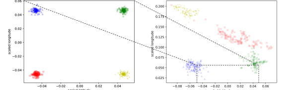
(a) Iteration 30

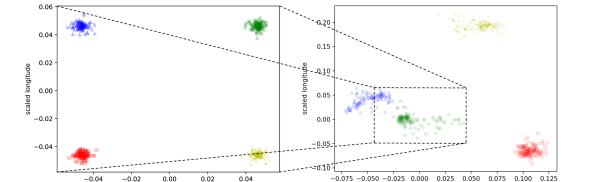
(b) Iteration 40

Figure 4: Using cross entropy for producing the noise does not make the system converge. The left sides of Figures (a) and (b) show the original synthetic data without noise. The right sides show the noisy data at different iterations. $L=270$m.

Figure 5: Synthetic testing data. From left to right: Laplace noise, no noise, our noise produced using mutual information. $L=270$m.

Number of cells
$13\times 13$	$65\times 65$	$130\times 130$	$260\times 260$
$0.75$	$0.00$	$0.00$	$0.00$

(a) Training data.

Number of cells
$13\times 13$	$65\times 65$	$130\times 130$	$260\times 260$
$0.75$	$0.00$	$0.00$	$0.00$

(b) Testing data.

Figure 6: Estimation of $B(X\mid Z)$ on the original version of the synthetic data.

	Number of cells
	$13\times 13$		$65\times 65$		$130\times 130$		$260\times 260$
Obf	Lap	Our	Lap	Our	Lap	Our	Lap	Our
$10$	$\pagecolor{lightgray}0.60$	$0.75$	$\pagecolor{lightgray}0.40$	$0.75$	$\pagecolor{lightgray}0.38$	$0.75$	$\pagecolor{lightgray}0.35$	$0.73$
$100$	$\pagecolor{lightgray}0.60$	$0.75$	$\pagecolor{lightgray}0.41$	$0.75$	$\pagecolor{lightgray}0.40$	$0.75$	$\pagecolor{lightgray}0.39$	$0.74$
$200$	$\pagecolor{lightgray}0.60$	$0.75$	$\pagecolor{lightgray}0.41$	$0.75$	$\pagecolor{lightgray}0.40$	$0.75$	$\pagecolor{lightgray}0.39$	$0.74$
$500$	$\pagecolor{lightgray}0.60$	$0.75$	$\pagecolor{lightgray}0.41$	$0.75$	$\pagecolor{lightgray}0.40$	$0.75$	$\pagecolor{lightgray}0.40$	$0.74$

(a) Training data.

	Number of cells
	$13\times 13$		$65\times 65$		$130\times 130$		$260\times 260$
Obf	Lap	Our	Lap	Our	Lap	Our	Lap	Our
$10$	$\pagecolor{lightgray}0.59$	$0.75$	$\pagecolor{lightgray}0.38$	$0.75$	$\pagecolor{lightgray}0.36$	$0.75$	$\pagecolor{lightgray}0.26$	$0.73$
$100$	$\pagecolor{lightgray}0.60$	$0.75$	$\pagecolor{lightgray}0.40$	$0.75$	$\pagecolor{lightgray}0.39$	$0.75$	$\pagecolor{lightgray}0.37$	$0.74$
$200$	$\pagecolor{lightgray}0.60$	$0.75$	$\pagecolor{lightgray}0.41$	$0.75$	$\pagecolor{lightgray}0.39$	$0.75$	$\pagecolor{lightgray}0.38$	$0.74$
$500$	$\pagecolor{lightgray}0.60$	$0.75$	$\pagecolor{lightgray}0.41$	$0.75$	$\pagecolor{lightgray}0.40$	$0.75$	$\pagecolor{lightgray}0.39$	$0.74$

(b) Testing data.

Figure 7: Estimation of $B(X\mid Z)$ on synthetic data for the Laplace and our mechanisms, with $L=270$m. The empirical utility loss for training and testing data is $\approx 282.07\mbox{m}-298.40$m respectively for the Laplace and $\approx 219.70\mbox{m}-219.26$m for ours. The optimal mechanism gives ${B(X\mid Z)}=1-\nicefrac{{1}}{{4}}=0.75$.

IV-A1 Training $G$ wrt cross entropy

As discussed in Sec III-A, training $G$ wrt $\mathit{CE}(X,Y)$ is not sound. This is confirmed in the experiments by the fact that $G$ is failing to converge. Fig. 4 shows the distribution generated by $G$ in two different iterations of the game. We observe that, trying to fool the classifier $C$, the generator on the right-hand side has simply moved locations around, so that each class has been placed in a different area. This clearly confuses a classifier trained on the distribution of the left-hand side, however the correlation between labels and location is still evident. A classifier trained on the new $G$ can infer the labels as accurately as before.

As a consequence, after each iteration, the accuracy of the newly trained $C_{i}$ is always $1$, while the Bayes error $B(X|Z)$ is $0$. The generator fails to converge to a distribution that effectively protects the users’ privacy. We can hence conclude that the use of cross entropy is unsound for training $G$.

IV-A2 Training $G$ wrt mutual information

Using now $I(X;Y)$ for training $G$ (while still using the more efficient cross entropy for $C$, as explained in Sec III-A), we observe a totally different behaviour. After each iteration the accuracy of the classifier drops, showing that the generator produces meaningful noise. Around iteration $i=149$ the accuracy of $\mathit{C}_{i}$ becomes $\approx 0.25$ both over the training and the validation set. This means that $\mathit{C}_{i}$ just randomly predicts one of the four classes. We conclude that the noise injection is maximally effective, since $0.75$ is the maximum possible Bayes error. Hence we know that we can stop.

The result of our method, i.e., the final generator $G_{i}$, to the testing set is reported in Fig. 5(c). The empirical distortion is $\approx 219.26$m. This is way below the limit of $270$m set in (29), and it is due to the fact that to achieve the optimum privacy we probably do not need more than $\approx 220$m. In fact, the distance of the vertices from the center is $\approx 212$m, and even though some locations are further away (up to $45$m more), there are also locations that are closer, and that compensate the utility loss (which is a linear average measure).

For comparison, the result of the application of the planar Laplace to the testing set is illustrated in Fig. 5(a). The empirical distortion (i.e., the distortion computed on the sampled obfuscated locations) is $\approx 298.40$m, which is in line with the theoretical distortion formulated in (31).

From Fig. 5 we can see that, while the Laplace tends to “spread out” the obfuscated locations, our method tends to concentrate them into a single point (mode collapse), i.e., the mechanism is almost deterministic. This is due to the fact that the utility constraint is sufficiently loose to allow the noisy locations to be displaced enough so to overlap all in the same point. When the utility constraint is stricter, the mechanism is forced to be probabilistic (and the mode collapse does not happen anymore). For example, consider two individuals, $A$ and $B$, in locations $a$ and $b$ respectively, at distance $100$m, assume that $L=40$m. Assume also, for simplicity, that there are no other locations available. Then the optimal solution maps $a$ into $b$ with probability $\nicefrac{{2}}{{5}}$, and into itself with probability $\nicefrac{{3}}{{5}}$ and vice versa for $b$). Nevertheless, we can expect that our mechanism will tend to overlap the obfuscated locations of different classes, as much as allowed by the utility constraint. With the Laplace, on the contrary, the areas of the various classes remain pretty separated. This is reflected by the Bayes error estimation reported in Fig. 7.

We note that the Bayes error of the planar Laplace tend to decrease as the grid becomes finer. We believe that this is due to the fact that, with a coarse grid, there is an effect of confusion simply due to the large size of each cell. We remark that the behavior of our noise, on the contrary, is quite stable. Note that, when the grid is very coarse ($13\times 13$ cells) the Bayes error is $0.75$ already on the original data (cfr. Fig. 6), which must be due to the fact that all the vertices are in the same cell. While the Bayes error remains $0.75$ also with our obfuscation mechanism, with Laplace it decreases to $0.60$. The reason is that the noise scatters the locations in different cells, and they become, therefore distinguishable.

Figure 8: Synthetic testing data. From left to right: Laplace noise, no noise, our noise produced using mutual information. $L=173$m.

	Number of cells
	$13\times 13$		$65\times 65$		$130\times 130$		$260\times 260$
Obf	Lap	Our	Lap	Our	Lap	Our	Lap	Our
$10$	$\pagecolor{lightgray}0.64$	$\pagecolor{white}0.74$	$\pagecolor{lightgray}0.26$	$0.45$	$\pagecolor{lightgray}0.23$	$0.43$	$\pagecolor{lightgray}0.22$	$0.41$
$100$	$\pagecolor{lightgray}0.64$	$\pagecolor{white}0.74$	$\pagecolor{lightgray}0.26$	$0.45$	$\pagecolor{lightgray}0.24$	$0.43$	$\pagecolor{lightgray}0.23$	$0.42$
$200$	$\pagecolor{lightgray}0.64$	$\pagecolor{white}0.74$	$\pagecolor{lightgray}0.26$	$0.45$	$\pagecolor{lightgray}0.24$	$0.43$	$\pagecolor{lightgray}0.24$	$0.42$
$500$	$\pagecolor{lightgray}0.64$	$\pagecolor{white}0.74$	$\pagecolor{lightgray}0.26$	$0.45$	$\pagecolor{lightgray}0.24$	$0.43$	$\pagecolor{lightgray}0.24$	$0.42$

(a) Training data.

	Number of cells
	$13\times 13$		$65\times 65$		$130\times 130$		$260\times 260$
Obf	Lap	Our	Lap	Our	Lap	Our	Lap	Our
$10$	$\pagecolor{lightgray}0.63$	$\pagecolor{white}0.74$	$\pagecolor{lightgray}0.25$	$0.44$	$\pagecolor{lightgray}0.23$	$0.42$	$\pagecolor{lightgray}0.19$	$0.39$
$100$	$\pagecolor{lightgray}0.64$	$\pagecolor{white}0.74$	$\pagecolor{lightgray}0.26$	$0.45$	$\pagecolor{lightgray}0.24$	$0.43$	$\pagecolor{lightgray}0.23$	$0.42$
$200$	$\pagecolor{lightgray}0.64$	$\pagecolor{white}0.74$	$\pagecolor{lightgray}0.26$	$0.45$	$\pagecolor{lightgray}0.23$	$0.43$	$\pagecolor{lightgray}0.23$	$0.42$
$500$	$\pagecolor{lightgray}0.64$	$\pagecolor{white}0.74$	$\pagecolor{lightgray}0.26$	$0.45$	$\pagecolor{lightgray}0.23$	$0.43$	$\pagecolor{lightgray}0.23$	$0.42$

(b) Testing data

Figure 9: Estimation of $B(X\mid Z)$ on the synthetic data for the Laplace and for our mechanisms, with $L=173$m. The empirical utility loss for training and testing data is $\approx 170.53$m – $172.35$m respectively for the Laplace and $\approx 166.78$m – $171.50$m for ours. The optimal mechanism gives $B(X\mid Z)=0.50$, since the utility bound is large enough to let mixing the red and blue points, as well as the green and the yellow, but does not allow more confusion than that.

IV-B Experiment 2: stricter utility constraint

We are now interested in investigating how our method behaves when a stricter constraint on the utility loss is imposed. In order to do so, we run an experiment similar to the one in Section IV-A. We repeat the same steps but now we set $L$ and the privacy parameter (and consequently the distortion rate) of the planar Laplace as follows:

$$L=173\mbox{m}\qquad\epsilon=\frac{\ln 2}{60}\qquad\mathbb{L}[Z\mid W]\approx 173.12\mbox{m}$$ (32)

Similarly to the previous section, training $G$ wrt cross entropy fails to converge, producing generators that achieve no privacy protection. As a consequence, we only show the results of training $G$ wrt mutual information.

The result of the application of the Laplace mechanism is illustrated in Fig. 8(a). The empirical distortion is $\approx 172.35$m.

Following the same pattern as in Section IV-A, we train $\mathit{G}$ and $\mathit{C}$. The training of $\mathit{G}$ is performed for 30 epochs during each iteration with a batch size of 512 samples and a learning rate of 0.0001. The classifier $\mathit{C}$ is trained for 3000 epochs with a batch size of 512 samples and 0.001 as the value for the learning rate during each iteration. We are particularly interested in the 24th iteration where $\mathit{C}$’s performance is degraded by the obfuscation performed by $\mathit{G}$ trained during the previous iteration. Training $\mathit{C}$ with 32 samples batch size and learning rate set to 0.001 for 100 epochs with the obfuscated data gives the results reported in Table II.

Data	Accuracy	F1_score
Training data	$\approx 0.55$	$\approx 0.54$
Validation data	$\approx 0.53$	$\approx 0.53$
Test data	$\approx 0.52$	$\approx 0.51$

TABLE II: Summary of the experiment with our noise.

In this case, increasing the number of epochs does not improve the classification precision and makes $\mathit{C}$ more prone to overfitting.

The obfuscation provided by $\mathit{G}$ at the 24th iteration produces the distributions on the testing illustrated in Fig. 8(c). The empirical distortion is $\approx 171.50$m. The estimated Bayes error for the two mechanisms is reported in Fig. 9.

V Experiments on the Gowalla dataset

In the previous section we saw that our method behaves as expected in a simple synthetic dataset, producing an obfuscation mechanism that is close to the optimal one (when $G$ is trained wrt mutual information). We now study the behaviour of our method to real location data from the Gowalla dataset. Since cross entropy was shown to be unsound, we only present results using mutual information for training $G$.

The dataset

The dataset consists of data extracted from the Gowalla dataset [41], a collection of check-ins made available by the Gowalla location-based social network. Among all the provided features, only the users’ identifiers (classes), the latitude and longitude of the check-in locations are considered. The data are selected as follows:

1. we consider a squared region centered in 5, Boulevard de Sébastopol, Paris, France with 4500m long side;

2. we select the 6 users who checked in the region most frequently, we retain their locations and discard the rest;

3. we filter the obtained locations to reduce the overlapping of the data belonging to different classes by randomly selecting for each class 82 location samples for training and validation purpose, and 20 samples for the test.

We obtain $492$ pairs $(\mathit{locations},\mathit{id})$ to train and validate the model, and $120$ to test it. For each of these, the generator creates 10 pairs with noisy locations using different seeds. As usual, $G_{0}$ does it using the Laplace function, the other $G_{i}$’s use the mechanism learnt at the previous step $i-1$. Thus in total we obtain 4920 pairs for training and 1200 for testing. Fig.10 shows the result of the mechanism applied to the testing data, where each color corresponds to a different user.

Figure 10: Gowalla testing data. From left to right: Laplace noise, no noise, our noise produced using mutual information. $L=1150$m.

Number of cells
$13\times 13$	$65\times 65$	$130\times 130$	$260\times 260$
$0.12$	$0.06$	$0.04$	$0.03$

(a) Training data.

Number of cells
$13\times 13$	$65\times 65$	$130\times 130$	$260\times 260$
$0.11$	$0.04$	$0.03$	$0.03$

(b) Testing data.

Figure 11: Estimation of $B(X\mid Z)$ on the original version of the data from Gowalla.

	Number of cells
	$13\times 13$		$65\times 65$		$130\times 130$		$260\times 260$
Obf	Lap	Our	Lap	Our	Lap	Our	Lap	Our
$10$	$\pagecolor{lightgray}0.56$	$0.83$	$\pagecolor{lightgray}0.37$	$0.83$	$\pagecolor{lightgray}0.19$	$0.82$	$\pagecolor{lightgray}0.06$	$0.80$
$100$	$\pagecolor{lightgray}0.57$	$0.83$	$\pagecolor{lightgray}0.53$	$0.83$	$\pagecolor{lightgray}0.46$	$0.82$	$\pagecolor{lightgray}0.31$	$0.81$
$200$	$\pagecolor{lightgray}0.57$	$0.83$	$\pagecolor{lightgray}0.55$	$0.83$	$\pagecolor{lightgray}0.50$	$0.82$	$\pagecolor{lightgray}0.40$	$0.81$
$500$	$\pagecolor{lightgray}0.57$	$0.83$	$\pagecolor{lightgray}0.56$	$0.83$	$\pagecolor{lightgray}0.54$	$0.82$	$\pagecolor{lightgray}0.48$	$0.81$

(a) Training data.

	Number of cells
	$13\times 13$		$65\times 65$		$130\times 130$		$260\times 260$
Obf	Lap	Our	Lap	Our	Lap	Our	Lap	Our
$10$	$\pagecolor{lightgray}0.51$	$0.83$	$\pagecolor{lightgray}0.18$	$0.82$	$\pagecolor{lightgray}0.07$	$0.80$	$\pagecolor{lightgray}0.01$	$0.79$
$100$	$\pagecolor{lightgray}0.56$	$0.83$	$\pagecolor{lightgray}0.45$	$0.82$	$\pagecolor{lightgray}0.30$	$0.81$	$\pagecolor{lightgray}0.13$	$0.80$
$200$	$\pagecolor{lightgray}0.56$	$0.83$	$\pagecolor{lightgray}0.49$	$0.82$	$\pagecolor{lightgray}0.38$	$0.81$	$\pagecolor{lightgray}0.21$	$0.80$
$500$	$\pagecolor{lightgray}0.56$	$0.83$	$\pagecolor{lightgray}0.53$	$0.82$	$\pagecolor{lightgray}0.46$	$0.81$	$\pagecolor{lightgray}0.33$	$0.80$

(b) Testing data.

Figure 12: Estimation of $B(X\mid Z)$ on the Gowalla data for the Laplace and for our mechanisms, with $L=1150$m. The utility loss for training and testing data is $\approx 1127.83\mbox{m}-1132.63$m respectively for the Laplace and $\approx 961.38\mbox{m}-979.40$m for ours. The optimal mechanism gives $B(X\mid Z)=1-\nicefrac{{1}}{{6}}=0.83$.

Figure 13: Gowalla testing data. From left to right: Laplace noise, no noise, our noise produced using mutual information. $L=518$m.

V-A Experiment 3: relaxed utility constraint

In this experiment we study the case of a large upper bound on the utility loss, which would potentially allow to achieve the maximum utility. We set $L$ and the privacy parameter (and consequently $\mathbb{L}[Z\mid W]$) of the planar Laplace as follows:

$$L=1150\mbox{m}\qquad\epsilon=\frac{\ln 2}{400}\qquad\mathbb{L}[Z\mid W]\approx 1154.15\mbox{m}$$ (33)

The results for the Laplace and our method are illustrated in Fig.10. As we can see, the utility constraint is relaxed enough to allow our method to achieve the maximum privacy. As reported in Fig.12, indeed, the Bayes error is close to that of random guess, namely $1-\nicefrac{{1}}{{6}}\approx 0.83$. Fig. 11 shows the part of the Bayes error due to the discretization of the domain ${\cal Z}$. The planar Laplace, on the other hand, confirms the relatively limited level of privacy as observed in the synthetic data.

V-B Experiment 4: stricter utility constraint

We consider now a much tighter utility constraint, and we set the parameters of the planar Laplace as follows:

$$L=518\mbox{m}\qquad\epsilon=\frac{\ln 2}{180}\qquad\mathbb{L}[Z\mid W]\approx 519.37\mbox{m}$$ (34)

The results of the application of the Laplace and of our method to the testing data are shown in Fig. 13, and the Bayes error is reported in Fig. 14.

	Number of cells
	$13\times 13$		$65\times 65$		$130\times 130$		$260\times 260$
Obf	Lap	Our	Lap	Our	Lap	Our	Lap	Our
$10$	$\pagecolor{lightgray}0.38$	$0.50$	$\pagecolor{lightgray}0.29$	$0.42$	$\pagecolor{lightgray}0.20$	$0.37$	$\pagecolor{lightgray}0.27$	$0.08$
$100$	$\pagecolor{lightgray}0.39$	$0.51$	$\pagecolor{lightgray}0.36$	$0.44$	$\pagecolor{lightgray}0.34$	$0.43$	$\pagecolor{lightgray}0.27$	$0.40$
$200$	$\pagecolor{lightgray}0.39$	$0.51$	$\pagecolor{lightgray}0.36$	$0.44$	$\pagecolor{lightgray}0.35$	$0.43$	$\pagecolor{lightgray}0.31$	$0.41$
$500$	$\pagecolor{lightgray}0.38$	$0.51$	$\pagecolor{lightgray}0.37$	$0.44$	$\pagecolor{lightgray}0.36$	$0.43$	$\pagecolor{lightgray}0.34$	$0.42$

(a) Training data.

	Number of cells
	$13\times 13$		$65\times 65$		$130\times 130$		$260\times 260$
Obf	Lap	Our	Lap	Our	Lap	Our	Lap	Our
$10$	$\pagecolor{lightgray}0.34$	$0.47$	$\pagecolor{lightgray}0.20$	$0.36$	$\pagecolor{lightgray}0.08$	$0.35$	$\pagecolor{lightgray}0.03$	$0.12$
$100$	$\pagecolor{lightgray}0.37$	$0.49$	$\pagecolor{lightgray}0.32$	$0.41$	$\pagecolor{lightgray}0.25$	$0.38$	$\pagecolor{lightgray}0.15$	$0.32$
$200$	$\pagecolor{lightgray}0.37$	$0.48$	$\pagecolor{lightgray}0.33$	$0.41$	$\pagecolor{lightgray}0.30$	$0.39$	$\pagecolor{lightgray}0.21$	$0.35$
$500$	$\pagecolor{lightgray}0.37$	$0.49$	$\pagecolor{lightgray}0.35$	$0.42$	$\pagecolor{lightgray}0.32$	$0.40$	$\pagecolor{lightgray}0.28$	$0.38$

(b) Testing data.

Figure 14: Estimation of $B(X\mid Z)$ on the Gowalla data for the Laplace and for our mechanisms, with $L=518$m. The utility loss fort training and testing data is $\approx 523.40\mbox{m}-535.21$m respectively for the Laplace and $\approx 487.34\mbox{m}-502.89$m for ours. We could not compute the optimal mechanism due to the high complexity of the linear program.

As the grid becomes finer, both the planar Laplace and our method become more sensitive to the number of samples, in the sense that the (approximation of) the Bayes error grows considerably as the number of samples increases. This is not surprising: when the cells are small they tend to have a limited number of hits. Therefore the number of hits whose class is in minority (in a given cell), and hence not selected as the best guess, is limited. Note that these minority hits are those that contribute to the Bayes error.

VI Conclusion and future work

We have proposed a method based on adversarial nets to generate obfuscation mechanisms with a good tradeoff between privacy and utility. The crucial feature of our approach is that the target function to minimize is the mutual information rather than the cross entropy. We have applied our method to the case of location privacy, and experimented with a set of synthetic data and with data from Gowalla. We have compared the mechanism obtained via our approach with the planar Laplace, the typical mechanism used for geo-indistinguishability, obtaining favorable results.

Although the experiments here were limited to the case of location privacy, our setting is very general and can in principle be applied to any kind of sensitive and public data with finite domain. The same holds for the notion of utility: in this paper we have considered the distortion, i.e. the expected distance between the original value $w$ and its corresponding noisy version $z$, but our framework can accommodate any notion of loss on which the gradient descent is applicable. In the future we plan to explore the validity of our approach to other privacy scenarios and other loss utility functions. We also plan to study the estimation of mutual information by means of other functions which are more suitable for neural networks training in order to reduce the computational burden.

We also plan to explore the possibility of using other notions of privacy. In particular, we are considering using directly the Bayes error $B(X,Z)$ in the objective function. The main challenge is when the domain of $Z$ is too large, as it makes unfeasible to estimate accurately $B(X,Z)$. We are currently exploring an approach based on partitioning the domain of $Z$, so to reduce its cardinality. We are also interested in considering the notion $g$-vulnerability [42] which generalizes (the converse of) the Bayes error to the case in which the adversary’s attack is rewarded by a generic gain functions $g$. Our main challenge, however, is to extend our framework to deal with worst-case notions of privacy, such as differential privacy and geo-indistinguishability. To this end, we plan to start with a variant of differential privacy called Rényi differential privacy [43], which is formulated in terms of divergence, and explore the applicability of the learning-based method for estimating $f$-divergences proposed in [44].

Moreover we plan to enhance the flexibility of the constraint on distortion (in the loss function), by requiring it to be per user rather than global. More specifically, we aim at producing obfuscation mechanisms that satisfy constraints stating that the expected displacement for each user is at most up to a certain threshold. The motivation is that different users may have different requirements. Another potential application is to encompass a notion of fairness, that can be obtained by requiring that the threshold is the same for everybody.

VI-A Acknowledgement

This research was supported by DATAIA Convergence Institute as part of the “Programme d’Investissement d’Avenir” (ANR-17-CONV-0003), operated by Inria and CentraleSupélec. It was also supported by the ANR project REPAS, and by the Inria/DRI project LOGIS. The work of Palamidessi was supported by the project HYPATIA, funded by the European Research Council (ERC) under the European Union’s Horizon 2020 research and innovation program, grant agreement n. 835294.

VII Appendix

VII-A Proofs of the results in the paper

See 2

Proof.

Let us recall that

$$X\leftrightarrow W\leftrightarrow Z\leftrightarrow Y.$$ (35)

represents a Markov chain where:

• the relation between the two random variables $X$ and $W$ is defined by the data distribution $P_{X,W}$,

• the relation between $Z$ and $Y$ depends only on the chosen classifier according to $P_{Y|Z}$,

• the relation between $Z$ and $W$ can be described by the variable $P_{Z|W}$

If we consider $X$ as the secret input and $Y$ as the observable output of a stochastic channel, the mutual information between the two random variable can be expressed as

$$I(X;Y)=g(P_{Y|X}).$$ (36)

We know from [8] that $g(\cdot)$ is a convex function wrt $P_{Y|X}$. We can express $P_{Y|X}$ as:

$$P_{Y|X}(y|x)=\frac{\sum_{zw}P_{X,W}(x,w)P_{Z|W}(z|w)P_{Y|Z}(y|z)}{\sum_{w}P_{X,W}(x,w)}.$$ (37)

Eq. (37) represents a linear function of the variable $P_{Z|W}$ (all the other probabilities are constant). Hence $f(P_{Z|W})=g(h(P_{Z|W}))$ where $g(\cdot)$ is convex and $h(\cdot)$ is linear. The composition of a convex function with a linear one is a convex function and this concludes the proof. ∎

See 3

Proof.

Given that eq. 1 represents a Markov chain, $X\leftrightarrow Z\leftrightarrow Y$ represents one as well. From the data processing inequality it follows that:

$$I(X;Y)\leq I(X;Z)\,.$$ (38)

Hence we have:

$$\max_{C}I(X;Y)\leq I(X;Z)\,,$$ (39)

and therefore:

$$\min_{G}\max_{C}I(X;Y)\leq\min_{G}I(X;Z)\,.$$ (40)

∎

See 4

Proof.

$$B(X\mid Z)=$$

$$\sum_{z}P_{Z}(z)(1-\max_{x}P_{X|Z}(x\mid z))$$

$$=1-\sum_{z}P_{Z}(z)\max_{x}P_{X|Z}(x\mid z)$$

$$=1-\sum_{y}P_{Y}(y)\sum_{z}P_{Z|Y}(z|y)\max_{x}P_{X|Z}(x\mid z)$$

$$\leq 1-\sum_{y}P_{Y}(y)\max_{x}\sum_{z}P_{Z|Y}(z|y)P_{X|Z}(x\mid z)$$

$$=1-\sum_{y}P_{Y}(y)\max_{x}P_{X|Y}(x\mid y)$$

$$=B(X\mid Y)$$

∎

See 5

Proof.

$P_{XW}$ is fixed, and therefore $H(X)$ is fixed as well. Hence the goal of $C$ of maximizing $I(X;Y)$ reduces to maximizing $-H(X|Y)$. Consider two mechanisms, $P_{Z_{1}|W}$ and $P_{Z_{2}|W}$, and the distributions induced on $X$ by $Z_{1}$ and $Z_{2}$ respectively, namely $P_{X|Z_{1}}$ and $P_{X|Z_{2}}$. Consider the predictions $P_{Y_{1}|Z_{1}}$ and $P_{Y_{1}|Z_{2}}$ that $C$ obtains by minimizing the cross entropy with $P_{X|Z_{1}}$ and $P_{X|Z_{2}}$ respectively.

It is well known that $\operatorname*{argmin}_{Q}\mathit{CE}(P,Q)=P$, hence we have $P_{Y_{1}|Z_{1}}=P_{X|Z_{1}}$ and $P_{Y_{2}|Z_{2}}=P_{X|Z_{2}}$. (Note that $X$, $Y_{1}$ and $Y_{2}$ all have the same domain ${\cal X}$.) Hence, taking into account that $X\leftrightarrow Z_{1}\leftrightarrow Y_{1}$ and $X\leftrightarrow Z_{2}\leftrightarrow Y_{2}$ (i.e., they are Markov chains), we have:

$$\scriptsize\begin{array}[]{c}-H(X|Y_{1})\leq-H(X|Y_{2})\\ \\[-3.01389pt] \mbox{iff}\\ \\[-3.01389pt] \sum_{z}P_{Z_{1}}(z)\sum_{xy}\,P_{X|Z_{1}=z}(x|z)P_{Y_{1}|Z_{1}=z}(y|z)\log P_{Y_{1}|Z_{1}=z}(y|z)\\ \leq\\ \sum_{z}P_{Z_{2}}(z)\sum_{xy}\,P_{X|Z_{2}=z}(x|z)P_{Y_{2}|Z_{2}=z}(y|z)\log P_{Y_{2}|Z_{2}=z}(y|z)\\ \\[-3.01389pt] \mbox{iff}\\ \\[-3.01389pt] \sum_{z}P_{Z_{1}}(z)\sum_{xy}\,P_{X|Z_{1}=z}(x|z)P_{X|Z_{1}=z}(y|z)\log P_{X|Z_{1}=z}(x|z)\\ \leq\\ \sum_{z}P_{Z_{2}}(z)\sum_{xy}\,P_{X|Z_{2}=z}(x|z)P_{X|Z_{2}=z}(y|z)\log P_{X|Z_{2}=z}(x|z)\\ \\[-3.01389pt] \mbox{iff}\\ \\[-3.01389pt] -H(X|Z_{1})\leq-H(X|Z_{2}).\end{array}$$

Finally, observe that

$$\scriptsize-H(X|Z_{1})\,\leq\,-H(X|Z_{2})\quad\mbox{implies}\quad\max_{P_{Y_{1}|Z}}I(X;Y_{1})\,\leq\,\max_{P_{Y_{2}|Z}}I(X;Y_{2})$$ (41)

and recall that $P_{Y_{i}|Z}$ is the prediction produced by $C$. ∎

See 6

Proof.

Let $P_{Y\mid Z}=\operatorname*{argmin}_{\mathit{C}}\;\mathit{CE}(X,Y)$ and let $f^{*}$ be defined as in (15). We note that, for every $z\in{\cal Z}$:

$$\begin{array}[]{l}\sum_{x}P_{X\mid Z}(x|z)\overline{\mathbb{1}}_{f^{*}}(x,z)\\ \begin{array}[]{cl}=&{\displaystyle\sum_{x\neq f^{*}(z)}P_{X|Z}(x,z)}\\ =&{\displaystyle\sum_{x\neq\operatorname*{argmax}_{y}P_{Y|Z}(y|z)}P_{X|Z}(x,z)}\\ =&1-{\displaystyle\sum_{x=\operatorname*{argmax}_{y}P_{Y|Z}(y|z)}P_{X|Z}(x,z)}\\ =&1-P_{X|Z}(\operatorname*{argmax}_{x}P_{X|Z}(x|z)\mid z))\\ =&1-\max_{x}P_{X|Z}(x\mid z))\\ \end{array}\end{array}$$

where the first equality is due to the definition of $\overline{\mathbb{1}}_{f^{*}}$, the second one is due to the definition of $f^{*}$, and the last but one follows from the fact that $P_{Y\mid Z}=\operatorname*{argmin}_{\mathit{C}}\;\mathit{CE}(X,Y)$ and therefore, by 5, $P_{Y\mid Z}=P_{X\mid Z}$. Hence, we have:

$$\begin{array}[]{l}{R(f^{*})}\\ \begin{array}[]{cl}=&\sum_{xz}P_{X,Z}(x,z)\overline{\mathbb{1}}_{f}^{*}(x,z)\\ =&\sum_{xz}P_{Z}(z)P_{X|Z}(x|z)\overline{\mathbb{1}}_{f}^{*}(x,z)\\ =&\sum_{z}P_{Z}(z)\sum_{x}P_{X|Z}(x|z)\overline{\mathbb{1}}_{f}^{*}(x,z)\\ =&\sum_{z}P_{Z}(z)(1-\max_{x}P_{X|Z}(x\mid z))\\ =&B(X\mid Z)\qquad\mbox{(cfr. \autoref{def:BayesError})}\end{array}\end{array}$$

∎

References

- [1] M. Fredrikson, S. Jha, and T. Ristenpart, “Model inversion attacks that exploit confidence information and basic countermeasures,” in Proc. of CCS, ser. CCS ’15. ACM, 2015, pp. 1322–1333.
- [2] R. Shokri, M. Stronati, C. Song, and V. Shmatikov, “Membership inference attacks against machine learning models,” in Proc. of S&P. IEEE Computer Society, 2017, pp. 3–18.
- [3] A. Pyrgelis, C. Troncoso, and E. D. Cristofaro, “Knock knock, who’s there? membership inference on aggregate location data,” in Proc. of NDSS. The Internet Society, 2018.
- [4] J. Hayes, L. Melis, G. Danezis, and E. D. Cristofaro, “LOGAN: membership inference attacks against generative models,” PoPETs, vol. 2019, no. 1, pp. 133–152, 2019.
- [5] L. Melis, C. Song, E. D. Cristofaro, and V. Shmatikov, “Exploiting unintended feature leakage in collaborative learning,” in Proc. of S&P. IEEE, 2019, pp. 497–512.
- [6] R. Shokri, G. Theodorakopoulos, and C. Troncoso, “Privacy games along location traces: A game-theoretic framework for optimizing location privacy,” ACM Trans. on Privacy and Security, vol. 19, no. 4, pp. 11:1–11:31, 2017.
- [7] N. E. Bordenabe, K. Chatzikokolakis, and C. Palamidessi, “Optimal geo-indistinguishable mechanisms for location privacy,” in Proc. of CCS, 2014.
- [8] T. M. Cover and J. A. Thomas, Elements of Information Theory, 2nd ed. J. Wiley & Sons, Inc., 2006.
- [9] M. E. Andrés, N. E. Bordenabe, K. Chatzikokolakis, and C. Palamidessi, “Geo-indistinguishability: differential privacy for location-based systems,” in Proc. of CCS. ACM, 2013, pp. 901–914.
- [10] K. Chatzikokolakis, E. ElSalamouny, and C. Palamidessi, “Efficient utility improvement for location privacy,” Proceedings on Privacy Enhancing Technologies (PoPETs), vol. 2017, no. 4, pp. 308–328, 2017.
- [11] R. Shokri, “Privacy games: Optimal user-centric data obfuscation,” Proceedings on Privacy Enhancing Technologies, vol. 2015, no. 2, pp. 299–315, 2015.
- [12] S. Oya, C. Troncoso, and F. Pérez-González, “Back to the drawing board: Revisiting the design of optimal location privacy-preserving mechanisms,” in Proc. of CCS. ACM, 2017, pp. 1959–1972.
- [13] I. Goodfellow, J. Pouget-Abadie, M. Mirza, B. Xu, D. Warde-Farley, S. Ozair, A. Courville, and Y. Bengio, “Generative adversarial nets,” in Advances in Neural Information Processing Systems 27. Curran Associates, Inc., 2014, pp. 2672–2680.
- [14] M. Abadi and D. G. Andersen, “Learning to protect communications with adversarial neural cryptography,” CoRR, vol. abs/1610.06918, 2016.
- [15] N. Santhi and A. Vardy, “On an improvement over Rényi’s equivocation bound,” 2006, presented at the 44-th Annual Allerton Conf. on Communication, Control, and Computing, September 2006. Available at http://arxiv.org/abs/cs/0608087.
- [16] Y. Zhu and R. Bettati, “Anonymity vs. information leakage in anonymity systems,” in Proc. of ICDCS. IEEE, 2005, pp. 514–524.
- [17] K. Chatzikokolakis, C. Palamidessi, and P. Panangaden, “On the Bayes risk in information-hiding protocols,” J. of Comp. Security, vol. 16, no. 5, pp. 531–571, 2008.
- [18] A. McIver, L. Meinicke, and C. Morgan, “Compositional Closure for Bayes Risk in Probabilistic Noninterference,” in Proc. of ICALP, ser. LNCS, vol. 6199. Springer, 2010, pp. 223–235.
- [19] G. Cherubin, “Bayes, not naïve: Security bounds on website fingerprinting defenses,” PoPETs, vol. 2017, no. 4, pp. 215–231, 2017.
- [20] M. S. Alvim, K. Chatzikokolakis, A. McIver, C. Morgan, C. Palamidessi, and G. Smith, “Axioms for information leakage,” in Proc. of CSF, 2016, pp. 77–92.
- [21] G. Smith, “On the foundations of quantitative information flow,” in Proc. of FOSSACS, ser. LNCS, vol. 5504. Springer, 2009, pp. 288–302.
- [22] C. Dwork, F. Mcsherry, K. Nissim, and A. Smith, “Calibrating noise to sensitivity in private data analysis,” in Proc. of TCC, ser. LNCS, vol. 3876. Springer, 2006, pp. 265–284.
- [23] J. C. Duchi, M. I. Jordan, and M. J. Wainwright, “Local privacy and statistical minimax rates,” in Proc. of FOCS. IEEE Computer Society, 2013, pp. 429–438.
- [24] K. Chatzikokolakis, M. E. Andrés, N. E. Bordenabe, and C. Palamidessi, “Broadening the scope of Differential Privacy using metrics,” in Proc. of PETS, ser. LNCS, vol. 7981. Springer, 2013, pp. 82–102.
- [25] M. S. Alvim, M. E. Andrés, K. Chatzikokolakis, and C. Palamidessi, “On the relation between Differential Privacy and Quantitative Information Flow,” in Proc. of ICALP, ser. LNCS, vol. 6756. Springer, 2011, pp. 60–76.
- [26] A. De, “Lower bounds in differential privacy,” in Proc. of TCC. Springer, 2012, pp. 321–338.
- [27] P. Cuff and L. Yu, “Differential privacy as a mutual information constraint,” in Proc. of CCS, ser. CCS ’16. ACM, 2016, pp. 43–54.
- [28] A. Tripathy, Y. Wang, and P. Ishwar, “Privacy-preserving adversarial networks,” CoRR, vol. abs/1712.07008, 2017.
- [29] C. Huang, P. Kairouz, X. Chen, L. Sankar, and R. Rajagopal, “Context-aware generative adversarial privacy,” Entropy, vol. 19, no. 12, 2017.
- [30] J. Jia and N. Z. Gong, “Attriguard: A practical defense against attribute inference attacks via adversarial machine learning,” in 27th USENIX Security Symposium (USENIX Security 18). USENIX Association, 2018, pp. 513–529.
- [31] J. Hamm, “Minimax filter: Learning to preserve privacy from inference attacks,” J. Mach. Learn. Res., vol. 18, no. 1, pp. 4704–4734, 2017.
- [32] J. Hayes and O. Ohrimenko, “Contamination attacks and mitigation in multi-party machine learning,” in Proc. of NIPS. Curran Associates Inc., 2018, pp. 6604–6616.
- [33] H. Edwards and A. J. Storkey, “Censoring representations with an adversary,” in Proc. of ICLR, 2016.
- [34] Z. Ren, Y. J. Lee, and M. S. Ryoo, “Learning to anonymize faces for privacy preserving action detection,” in Proc. of ECCV, ser. LNCS, vol. 11205. Springer, 2018, pp. 639–655.
- [35] B. K. Beaulieu-Jones, Z. S. Wu, C. Williams, R. Lee, S. P. Bhavnani, J. B. Byrd, and C. S. Greene, “Privacy-preserving generative deep neural networks support clinical data sharing,” Circulation: Cardiovascular Quality and Outcomes, vol. 12, no. 7, p. e005122, 2019.
- [36] M. I. Belghazi, A. Baratin, S. Rajeshwar, S. Ozair, Y. Bengio, A. Courville, and D. Hjelm, “Mutual information neural estimation,” in Proceedings of the 35th Int. Conf. on Machine Learning, ser. Proceedings of Machine Learning Research, vol. 80. PMLR, 2018, pp. 531–540.
- [37] S. Nowozin, B. Cseke, and R. Tomioka, “f-gan: Training generative neural samplers using variational divergence minimization,” in Proc. of NIPS, 2016, pp. 271–279.
- [38] Y. O. Basciftci, Y. Wang, and P. Ishwar, “On privacy-utility tradeoffs for constrained data release mechanisms,” in Proc. of ITA. IEEE, 2016, pp. 1–6.
- [39] X. Glorot and Y. Bengio, “Understanding the difficulty of training deep feedforward neural networks,” in Proceedings of the Thirteenth Int. Conf. on AI and Statistics, ser. Proceedings of Machine Learning Research, vol. 9. PMLR, 2010, pp. 249–256.
- [40] N. S. Keskar, D. Mudigere, J. Nocedal, M. Smelyanskiy, and P. T. P. Tang, “On large-batch training for deep learning: Generalization gap and sharp minima,” CoRR, vol. abs/1609.04836, 2016.
- [41] J. Leskovec and A. Krevl, “The Gowalla dataset (Part of the SNAP collection),” https://snap.stanford.edu/data/loc-gowalla.html.
- [42] M. S. Alvim, K. Chatzikokolakis, C. Palamidessi, and G. Smith, “Measuring information leakage using generalized gain functions,” in Proc. of CSF, 2012, pp. 265–279.
- [43] I. Mironov, “Rényi differential privacy,” in Proc. of CSF, 2017, pp. 263–275.
- [44] P. K. Rubenstein, O. Bousquet, J. Djolonga, C. Riquelme, and I. O. Tolstikhin, “Practical and consistent estimation of f-divergences,” in Proc. of NIPS, 2019, pp. 4072–4082.