Tree Boosted Varying Coefficient Models

Abstract

This paper investigates the integration of gradient boosted decision trees and varying coefficient models. We introduce the tree boosted varying coefficient framework which justifies the implementation of decision tree boosting as the nonparametric effect modifiers in varying coefficient models. This framework requires no structural assumptions in the space containing the varying coefficient covariates, is easy to implement, and keeps a balance between model complexity and interpretability. To provide statistical guarantees, we prove the asymptotic consistency of the proposed method under the regression settings with $L^{2}$ loss. We further conduct a thorough empirical study to show that the proposed method is capable of providing accurate predictions as well as intelligible visual explanations.

1 Introduction

In this paper we study the amalgamation of gradient boosting, especially gradient boosted decision trees (GBDT or GBM: Friedman, 2001), and varying coefficient models (VCM: Hastie and Tibshirani, 1993). A varying coefficient model is a semi-parametric model with coefficients that change along with each input. Under a general statistical learning setting with a set of covariates and some response of interest, a VCM isolates part of those covariates as effect modifiers based on which model coefficients are determined through a few varying coefficient mappings. These coefficients then get joined with the remaining covariates to generate a parametric prediction. To elaborate, consider performing least square regression on $(X,Z,Y)\in\mathbb{R}^{p}\times\mathbb{A}\times\mathbb{R},i=1,\dots,n$ where $X=(X^{1},\dots,X^{p})$, $X$ and $Z$ are the covariates and $Y$ the response. One VCM regression can take the form of

$$g(\mathbb{E}\left[{Y|X,Z}\right])=\beta^{0}(Z)+\sum_{i=1}^{p}\beta^{i}(Z)X^{i},$$ (1)

with the parametric part being a generalized linear model with the link function $g$. In this context we would like to refer to $X$ as the predictive covariates and $Z$ the action covariates (effect modifiers) which are drawn from $\mathbb{A}$ the action space. $\beta^{i}(\cdot):\mathbb{A}\to\mathbb{R},i=0,1,\dots,p$ are, conventionally nonparametric, varying coefficient mappings. While (1) maintains the linear structure, due to the dependence of $\beta$ on any given $Z$, the model belongs to a more complicated and flexible model space rather than the corresponding generalized linear model.

Our proposed model, tree boosted VCM, utilizes ensembles of gradient boosted decision trees as the varying coefficient mappings $\beta$. To demonstrate, for each $\beta^{i},i=0,\dots,p$, let

$$\beta^{i}(z)=\sum_{j=1}^{b}t^{i}_{j}(z),$$

an additive boosted tree ensemble of size $b$ with each $t_{j}^{i}$ a decision tree constructed sequentially through gradient boosting. We will postpone the details of model construction to Section 2. This strategy yields a model of

$$g(\mathbb{E}\left[{Y|X,Z}\right])=\sum_{j=1}^{b}t^{0}_{j}(Z)+\sum_{i=1}^{p}\left(\sum_{j=1}^{b}t^{i}_{j}(Z)\right)X^{i}.$$ (2)

Introducing VCM aligns with our attempt to answer the rising concern about model intelligibility and transparency, around which there are two branches of methods. We can either apply post hoc methods such that state-of-the-art “black box” models are constructed before we grant them meanings through analyzing their results. There is a sizable literature on this topic, from the appearance of local methods (Ribeiro et al., 2016) to recent applications on neural nets (Zhang and Zhu, 2018), random forests (Mentch and Hooker, 2016; Basu et al., 2018) and complex model distillation (Lou et al., 2012, 2013; Tan et al., 2017). However, objectivity is one inevitable challenge of tying explanations to models, especially in the presence of plentiful universal local methods capable of dealing with most models. Any use of post hoc analysis may be subject to justify the chosen explanatory method over the others, which is likely to add an additional explanation selection phase on top of the existing model selection.

On the other hand, another branch of methods attempts to build interpretability into model structures, meaning that models should be the integration of simple and intelligible building blocks that they become accountable by human inspection once trained. Examples of this range from simple models as generalized linear models and decision trees, to models that guarantee monotonicity (You et al., 2017; Chipman et al., 2016) or have identifiable components (Melis and Jaakkola, 2018). Although having the advantage of not requiring post hoc examination, in contrast to the aforementioned methods, self-explanatory models are restricted by their possible model complexity and flexibility, potentially limiting their accuracy. This lack of flexibility also implies that such a model, unless possessing a granular structure, may only provide global interpretation because all observations are reasoned via an identical procedure. Such behavior prevents us from zooming into a small region in the sample space.

Following this discussion, VCM belongs to the second category as long as the involved parametric models are intelligible. It is an instant generalization of parametric methods to allow the use of local coefficients, which leads to improvements in model complexity and accuracy, whereas the predictions are still produced through parametric relations between predictive covariates and coefficients. This combination demonstrates a feasible means to balance the trade-off between flexibility and intelligibility.

A great amount of research has been conducted to study the asymptotic properties of different VCMs when splines or kernel smoothers are implemented as the nonparametric varying coefficient mappings. We refer the readers to Park et al. (2015) for a comprehensive review. In this paper we intend to conclude similar results regarding the asymptotics of tree boosted VCM.

1.1 Models under VCM

Under the settings of (1), Hastie and Tibshirani (1993) pointed out that VCM is the generalization of generalized linear models, generalized additive models, and various other semi-parametric models with careful choices of the varying coefficient mapping $\beta$.

We would like to mention two special cases that have drawn our attention. One is the functional trees introduced in Gama (2004). A functional tree segments the action space into disjoint regions, after which a parametric model gets fitted within each region using sample points inside. Logistic regression trees, for which there is a sophisticated building algorithm (LOTUS: Chan and Loh, 2004), belong to such model family. Their prediction on $(x_{0},z_{0})$ is

$$P(\hat{y}_{0}=1)=\sum_{i=1}^{K}\frac{1}{1+e^{-x_{0}^{T}\beta_{i}}}\cdot I\left(z_{0}\in A_{i}\right)=\frac{1}{1+e^{-x_{0}^{T}\beta_{k}}},$$

provided $\mathbb{A}=\coprod_{i=1}^{K}A_{i}$ the tree segmentation, $z_{0}\in A_{k}$ and $\beta_{k}=\beta(z),\forall z\in A_{k}$. The conventional approach to determine functional tree structure is to recursively enumerate through candidate splits and choose the one that reduces the training loss the most between before and after splitting. Despite of the guaranteed stepwise improvement, such greedy strategy has the side effect of being both time consuming and mathematically intractable.

Another case is the partially linear regression that assumes

$$Y=X^{T}\beta+f(Z)+\epsilon_{Z},\quad\epsilon_{Z}\sim N(0,\sigma^{2}(Z)),$$

where $\beta$ is a global linear coefficient (see Härdle et al., 2012). It is equivalent to a least square VCM with all varying coefficient mappings except the intercept being constant.

1.2 Trees and VCM

While popular choices of varying coefficient mappings are either splines or kernel smoothers, it is a natural transition to consider exercising decision trees (CART: Breiman et al., 1984) and decision tree ensembles to serve as these nonparametric mappings. Using trees enables us to work adaptively with any action space $\mathbb{A}$ compatible with decision tree splitting logic, for example an arbitrary high dimensional mixture of continuous and discrete quantities, whereas traditional methods require to craft model structures case by case depending on the given $\mathbb{A}$.

We start with the straightforward attempts to utilize a single decision tree as varying coefficient mappings (Buergin and Ritschard, 2017; Berger et al., 2017). Although having a simple form, these implementations are also subject to the instability caused by the greedy tree building algorithm. Moreover, the mathematical intractability of decision trees prevents these single-tree based varying coefficient mappings from provable optimality. This instead suggests implementations through tree ensembles of either random forests or gradient boosting. One example is to use the linear local forests introduced in Friedberg et al. (2018) that perform local linear regression with an honest random forest kernel, while the predictive covariates $X$ are reused as the action covariates $Z$. In terms of boosting methods, Wang and Hastie (2014) proposed the first tree boosted VCM algorithm. They reduced the empirical risk by boosting using functional trees to fit the residuals to improve model coefficients, resulting in models of

$$g(\mathbb{E}\left[{Y|X,Z}\right])=\left(\sum_{j=1}^{b}t_{j}(Z)\right)^{T}(1,X),$$

where each $t_{j}$ returns a $(p+1)$ dimensional response. However, building a functional tree ensemble requires the construction and comparison of massive amounts of submodels and the joint optimization of all coefficients. In contrast, we aim to perform gradient boosting down on the coefficient level to comply with the standard boosting framework in order to separate the coefficients and to make tree boosted VCM coherent with existing boosting theories.

In the following sections, we explore the feasibility and statistical properties of adopting generic gradient boosted decision trees to serve as the nonparametric varying coefficient mappings for VCM. In Section 2, we share the perspective of analyzing such models as local gradient descent which creates functional coefficients and optimizes using local information. We will prove the consistency of this method in Section 3 and present a few empirical study results in Section 4. Further discussions on potential variations of this method follow in Section 5.

2 Tree Boosted Varying Coefficient Models

2.1 Notations

We will use the following notations in our discussion. We use superscripts $0,\dots,p$ to indicate individual components, i.e. $\beta=(\beta^{0},\dots,\beta^{p})^{T}$, and subscripts $1,\dots,n$ to indicate sample points or boosting iterations. For any $X$ when there is no ambiguity we assume $X$ contains the intercept column, i.e. $X=(1,X^{1},\dots,X^{p})$, so that $X^{T}\beta=\beta^{0}+\sum_{i=1}^{p}X^{i}\beta^{i}$ can be used to specify a linear regression.

2.2 Boosting Framework

We start by looking at a parametric generalized linear model with coefficients $\beta\in\mathbb{R}^{p+1}$ using gradient descent. Given sample $(x_{1},z_{1},y_{1}),\dots,(x_{n},z_{n},y_{n})$ and a loss function $l$, gradient descent minimizes the empirical risk to search for the optimal $\hat{\beta}^{*}$ as

$$L(\hat{\beta})=\frac{1}{n}\sum_{i=1}^{n}l(y_{i},x_{i}^{T}\hat{\beta}),\quad\hat{\beta}^{*}=\arg\min_{\hat{\beta}}L(\hat{\beta}).$$

To improve an interim $\hat{\beta}$, we move it in the negative gradient direction

$$\Delta_{\hat{\beta}}=\nabla_{\beta}L=-\nabla_{\beta}\left(\frac{1}{n}\sum_{i=1}^{n}l(y_{i},x_{i}^{T}\beta)\Big{|}_{\beta=\hat{\beta}}\right),$$

to obtain a new iteration $\hat{\beta}^{\prime}=\hat{\beta}+\lambda\Delta_{\hat{\beta}}$ for a positive and small learning rate $\lambda\ll 1$.

In order to extend this setting to varying coefficient models, we instead consider $\beta$ to be a mapping $\beta=\beta(z):\mathbb{A}\to\mathbb{R}^{p+1}$ so that it will apply to the covariates based on their values in the action space. Writing estimate of $\beta$ by $\hat{\beta}:\mathbb{A}\to\mathbb{R}^{p+1}$, the empirical risk remains a similar form

$$L(\hat{\beta})=\frac{1}{n}\sum_{i=1}^{n}l(y_{i},x_{i}^{T}\hat{\beta}(z)).$$

We perform the same gradient calculation as above, but only pointwisely for now. It produces the negative gradient direction at the point $z_{i}$

$$\Delta_{\beta}(z_{i})=-\nabla_{\beta}l(y_{i},x_{i}^{T}\beta)\Big{|}_{\beta=\hat{\beta}(z_{i})}.$$ (3)

As a result, we get the functional improvement of $\hat{\beta}$ captured at each of the sample points, i.e. $(z_{1},\Delta_{\beta}(z_{1})),\dots,(z_{n},\Delta_{\beta}(z_{n}))$. This observation leads us to employ gradient descent in functional space, also known as boosting (Friedman, 2001). For any function family $\mathcal{T}$ capable of regressing $\Delta_{\beta}(z_{1}),\dots,\Delta_{\beta}(z_{n})$ on $z_{1},\dots,z_{n}$, the corresponding ordinary boosting framework works as follows.

1. Start with an initial guess of $\hat{\beta}_{0}(\cdot)$.

2. For each component $j=0,\dots,p$ of $\hat{\beta}_{b},b\geq 0$, we calculate the pseudo gradient at each point as

   $$\Delta^{j}_{\beta_{i}}=-\frac{\partial{l(y_{i},x_{i}^{T}\beta)}}{\partial{\beta^{j}}}\Big{|}_{\beta=\hat{\beta}_{b}(z_{i})},$$

   for $i=1,\dots,n$.

3. For each $j$, find a good fit $t_{b+1}^{j}\in\mathcal{T}:\mathbb{A}\to\mathbb{R}$ on $(z_{i},\Delta^{j}_{\beta_{i}}),i=1,\dots,n$.

4. Update $\hat{\beta}_{b}$ with learning rate $\lambda\ll 1$.

   $$\hat{\beta}_{b+1}(\cdot)=\hat{\beta}_{b}(\cdot)+\lambda\begin{bmatrix}t_{b+1}^{0}(\cdot)\\ \vdots\\ t_{b+1}^{p}(\cdot)\end{bmatrix}.$$

When the spline method is implemented, $\mathcal{T}$ is closed under addition so that we will expect the result of (B4) to be expressed as a set of coefficients of basis functions for $\mathcal{T}$. On the other hand, when we apply decision trees in place of (B3):

1. For each $j$, build a decision tree $t_{b+1}^{j}:\mathbb{A}\to\mathbb{R}$ on $(z_{i},\Delta^{j}_{\beta_{i}}),i=1,\dots,n$,

the resulting varying coefficient mapping will be an additive tree ensemble, whose model space varies based on the ensemble size. We will refer to this method as tree boosted VCM.

Notice that the strategy of building a decision tree in (B3’) influences the properties of the obtained tree boosted VCM. The standard CART strategy executes as follows.

1. Start at the root node.

2. Given a node, numerate candidate splits and evaluate them using all $(z_{i},\Delta^{j}_{\beta_{i}})$ such that $z_{i}$ is contained in the node.

3. Split on the best candidate split.

4. Keep splitting until stopping rules are met to form terminal nodes.

5. Calculate fitted terminal values in each terminal node using all $(z_{i},\Delta^{j}_{\beta_{i}})$ such that $z_{i}$ is contained in the terminal node.

Recent developments on decision trees also suggest alternative strategies that produce better theoretical guarantees. We may consider subsampling that generates a subset $w\subset\{1,\dots,n\}$ and only uses sample points indexed by $w$ in (D2).

1. Given a node, numerate candidate splits and evaluate them using all $(z_{i},\Delta^{j}_{\beta_{i}})$ such that $i\in w$ and $z_{i}$ is contained in the node.

We may also consider honesty (Wager and Athey, 2018) which avoids using the responses, in our case $\Delta^{j}_{\beta_{i}}$, twice during both deciding the tree structure and deciding terminal values. For instance, a version of completely random trees discussed in Zhou and Hooker (2018) chooses the splits using solely $z_{i}$ without evaluating the splits by the responses $\Delta^{j}_{\beta_{i}}$ in place of steps (D2) and (D3).

1. Given a node, choose a random split based on $z_{i}$’s contained in the node.

2.3 Local Gradient Descent with Tree Kernels

Decision tree fits in (B3’) generate local linear combinations of pseudo-gradients thanks to the grouping effect carried by decision tree terminal nodes. To elaborate from a generic viewpoint, for all tree building strategy we discussed above we can introduce a kernel smoother $K:\mathbb{A}\times\mathbb{A}\to\mathbb{R}$ such that the estimated gradient at any new $z$ is given by

$$\Delta_{\beta}(z)=-\sum_{i=1}^{n}\left(\nabla_{\beta}l(y_{i},x_{i}^{T}\beta)\Big{|}_{\beta=\hat{\beta}(z_{i})}\right)\cdot\frac{K(z,z_{i})}{\sum_{j=1}^{n}K(z,z_{j})}.$$ (4)

In other words, with a fast decaying $K$, (4) can estimate the gradient at $z$ locally using weights given by

$$S(z,z_{i})=\frac{K(z,z_{i})}{\sum_{j=1}^{n}K(z,z_{j})}.$$

We would like to define such method as local gradient descent.

During standard tree boosting employing CART strategy, after a decision tree is constructed each iteration, its induced smoother $K$ assigns equal weights to all sample points in the same terminal node. If we write $A(z_{i})\subset\mathbb{A}$ the region in the action space corresponding to the terminal node containing $z_{i}$, we have $K(z,z_{i})=I(z\in A(z_{i}))$ and we define the following

$$\mathbf{K}(z,z_{i})\triangleq S(z,z_{i})=\frac{I\left(z\in A(z_{i})\right)}{\sum_{j=1}^{n}I(z_{j}\in A(z_{i}))}$$

to be the tree structure function where we also use the convention that $0/0=0$. The denominator is the size of $z_{i}$’s terminal node and is equal to $\sum_{j=1}^{n}I(z_{j}\in A(z))$ when $z$ and $z_{i}$ fall in the same terminal node. In the cases where subsampling or completely random trees are employed for the purpose of variance reduction, $\mathbf{K}$ will be taken to be the expectation such that

$$\mathbf{K}(z,z_{i})\triangleq\mathbb{E}\left[{S(z,z_{i})}\right]=\mathbb{E}\left[{\frac{I(z\in A(z_{i}))I(i\in w)}{\sum_{j=1}^{n}I(z_{j}\in A(z_{i}))I(i\in w)I(j\in w)}}\right].$$

whose properties have been studied by Zhou and Hooker (2018). This expectation is taken over all possible tree structures and, if subsampling is applied, all possible subsamples $w$ of a fixed size, and the denominator in the expectation is again the size of $z_{i}$’s terminal node.

In particular, by carefully choosing the rates for tree construction, this tree structure function is related to the random forest kernel introduced in Scornet (2016) that takes the expectation of the numerator and the denominator separately as

$$\mathbf{K}_{RF}(z,z_{i})=\frac{\mathbb{E}\left[{I\left(z\in A(z_{i})\right)}\right]}{\mathbb{E}\left[{\sum_{j=1}^{n}I\left(z_{j}\in A(z_{i})\right)}\right]},$$

in the sense that the deviations from these expectations are mutually bounded by constants.

Gradient boosting applied under nonparametric regression setting has to be accompanied by regularization such as using a complexity penalty or early stopping to prevent overfitting. When decision trees are implemented as the base learners, the complexity penalty is implicitly embedded in the tree parameters such as tree depth and terminal node size, while early stopping can be enforced during training. In fact, while we keep the parametric linear structure in VCM, local neighborhood weighting used for fitting the nonparametric coefficient mappings still adds to the model complexity. Therefore moderate restrictions, especially growth rates, have to be applied to avoid building saturated models with respect to the action space.

2.4 Examples

Tree boosted VCM generates a two-phase model such that the varying coefficient mappings generate effect modifiers and these effect modifiers join with predictive covariates linearly. In order to understand the varying coefficient mappings on the actions space, we provide a visualized example here by considering the following data generating process:

$$X\sim\mbox{Unif}[0,1]^{3},Z=(Z^{1},Z^{2})\sim\mbox{Unif}[0,1]^{2},\epsilon\sim N(0,0.25),$$

$$Y=X^{T}\begin{bmatrix}1\\ 3\\ -5\end{bmatrix}\cdot I(Z^{1}+Z^{2}<1)+X^{T}\begin{bmatrix}0\\ 10\\ 0\end{bmatrix}\cdot I(Z^{1}+Z^{2}\geq 1)+\epsilon.$$

We generate a sample of size 1,000 from the above distribution, apply the tree boosted VCM with 400 trees, and obtain the following estimation of the varying coefficient mappings $\beta$ on $Z$ in Figure 1. Our fitted values accurately capture the true coefficients.

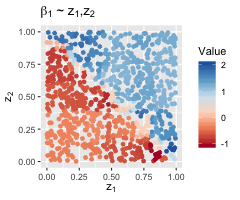
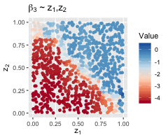
Figure 1: Example of varying coefficient mappings on the action space under the OLS settings.

Switching to logistic regression setting and assuming similarly that

$$\mbox{logit}P(Y=1)=\exp\left(X^{T}\begin{bmatrix}1\\ 3\\ -5\end{bmatrix}\cdot I(Z^{1}+Z^{2}<1)+X^{T}\begin{bmatrix}0\\ 10\\ 0\end{bmatrix}\cdot I(Z^{1}+Z^{2}\geq 1)\right),$$

with a sample of size 1,000, Figure 2 presents equivalent plots for our tree boosted VCM. These results are less clear since logistic regression produces more volatile gradients.

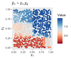
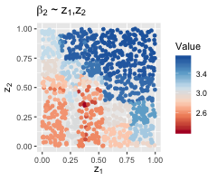
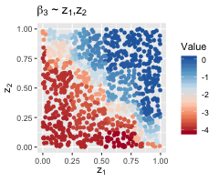
Figure 2: Example of varying coefficient mappings on the action space under the logistic regression settings.

In both cases our methods correctly identify $\beta(z)$ as segmenting along the diagonal in $z$, providing clear visual identification of the behavior of $\beta(z)$. These figures are evidence of the capability of tree boosted VCM to find the varying coefficients without posting structural assumptions on the action space. Further empirical studies are presented in Section 4.

3 Tree Boosted VCM Asymptotics

There is a large literature providing statistical guarantees and asymptotic analyses of different versions of VCM with varying coefficient mappings obtained via splines or local smoothers (Park et al., 2015; Fan et al., 1999, 2005). In this section we will demonstrate the asymptotic analyses of tree boosted VCM under mild conditions.

3.1 Tree Boosted VCM with $L^{2}$ Loss

Consider $L^{2}$ boosting setting for regression. Given the relationship

$$Y=f(X,Z)+\epsilon_{Z},\quad\epsilon_{Z}\sim N(0,\sigma^{2}_{Z}),$$

we work with the following assumptions.

1. Unit support of $X$ that $\mbox{supp }X=\{1\}\times[-1,1]^{p}$, which is achievable by standardizing without loss of generality for any finitely supported $X$.

2. Uniform bounded noise variance that $\sigma_{Z}\leq\sigma^{*}$.

3. $L^{2}$ loss that $L(u,y)=\frac{1}{2}(u-y)^{2}.$

Under these conditions, evaluating the pseudo-gradient given in (3) yields

$$\Delta_{\beta}(z_{i})=-\nabla_{\beta}l(y_{i},x_{i}^{T}\beta)\Big{|}_{\beta=\hat{\beta}(z_{i})}=(y_{i}-x_{i}^{T}\hat{\beta}(z_{i}))\cdot x_{i}.$$

For an existing terminal node $R\subseteq\mathbb{A}$, as per (4), the decision tree update in $R$ is

$$\Delta_{\beta}(z\in R)=\frac{\sum_{i=1}^{n}(y_{i}-x_{i}^{T}\hat{\beta}(z_{i}))\cdot x_{i}\cdot I\left(z_{i}\in R\right)}{\sum_{i=1}^{n}I\left(z_{i}\in R\right)},$$ (5)

and should subsample $w$ be present

$$\Delta_{\beta}(z\in R;w)=\frac{\sum_{i=1}^{n}(y_{i}-x_{i}^{T}\hat{\beta}(z_{i}))\cdot x_{i}\cdot I\left(z_{i}\in R\right)I\left(i\in w\right)}{\sum_{i=1}^{n}I\left(z_{i}\in R\right)I\left(i\in w\right)}.$$

3.2 Decomposing Decision Trees

We assume the action space $\mathbb{A}$ involves only continuous and categorical covariates, therefore we will consider its embedding into a Euclidean space $\mathbb{R}^{d}$ where $d=\mbox{dim}(\mathbb{A})$ is the dimension of the embedding. Denote $\mathcal{R}=\{(a_{1},b_{1}]\times\cdots\times(a_{d},b_{d}]|-\infty\leq a_{i}\leq b_{i}\leq\infty\}$ the collection of all hyper rectangles in $\mathbb{A}$. This set includes all possible terminal nodes of any decision tree built on $\mathbb{A}$. Given the distribution $(Z,1,X)\sim\mathbb{P}$, we define the inner product $\left\langle f_{1},f_{2}\right\rangle=\mathbb{E}_{\mathbb{P}}\left[{f_{1}f_{2}}\right],$ and the norm $\left\|\cdot\right\|=\left\|\cdot\right\|_{\mathbb{P},2}$ on the sample space $\mathbb{A}\times\{1\}\times[-1,1]^{p}$. For a sample of size $n$, we write the (unscaled) empirical counterpart by $\left\langle f_{1},f_{2}\right\rangle_{n}=\sum_{i=1}^{n}f_{1}(x_{i},z_{i})f_{2}(x_{i},z_{i}),$ such that $n^{-1}\left\langle f_{1},f_{2}\right\rangle_{n}\to\left\langle f_{1},f_{2}\right\rangle$ by the law of large numbers, with a corresponding norm $\left\|\cdot\right\|_{n}$.

Consider the following classes of functions on $\mathbb{A}\times\{1\}\times[-1,1]^{p}$.

• $\mathcal{H}=\left\{h_{R}(x,z)=I\left(z\in R\right)|R\in\mathcal{R}\right\}$, indicators of hyper rectangles.

• $\mathcal{G}=\left\{g_{R,j}(x,z)=I\left(z\in R\right)\cdot x^{j}|R\in\mathcal{R},j=0,\dots,p\right\}$ constants and coordinate mappings in hyper rectangles in $\mathcal{R}$. In particular we write $1=x^{0}$ so that $g_{R,0}=h_{R}$.

Bühlmann (2002) established a consistency guarantee for tree-type basis functions for $L^{2}$ boosting, in which the key point is to bound the gap between the boosting procedure and its population version by the uniform convergence in distribution of the family of indicators for hyper rectangles. We take a similar approach, for which we have to extend the uniform convergence to a broader function class defined as $\mathcal{G}$ as defined above. The following lemma provides uniform bounds on the asymptotic variability pertaining to $\mathcal{G}$ using Donsker’s theorem (see van der Vaart and Wellner, 1996).

Lemma 3.1.

For given $L^{2}$ function $f$ and random sub-Gaussian noise $\epsilon$, the following empirical gaps

1. $\xi_{n,1}=\sup_{R\in\mathcal{R}}\left|\left\|h_{R}\right\|^{2}-\frac{1}{n}\left\|h_{R}\right\|_{n}^{2}\right|,$

2. $\xi_{n,2}=\sup_{R\in\mathcal{R},j=0,\dots,p}\left|\left\|g_{R,j}\right\|^{2}-\frac{1}{n}\left\|g_{R,j}\right\|_{n}^{2}\right|,$

3. $\xi_{n,3}=\sup_{R\in\mathcal{R},j=0,\dots,p}\left|\left\langle f,g_{R,j}\right\rangle-\frac{1}{n}\left\langle f,g_{R,j}\right\rangle_{n}\right|,$

4. $\xi_{n,4}=\sup_{R\in\mathcal{R},j=0,\dots,p}\left|\frac{1}{n}\left\langle\epsilon,g_{R,j}\right\rangle_{n}\right|,$

5. $\xi_{n,5}=\sup_{R_{1},R_{2}\in\mathcal{R},j,k=0,\dots,p}\left|\left\langle g_{R_{1},j},g_{R_{2},k}\right\rangle-\frac{1}{n}\left\langle g_{R_{1},j},g_{R_{2},k}\right\rangle_{n}\right|,$

6. $\xi_{n,6}=\left|\frac{1}{n}\left\|f+\epsilon\right\|_{n}^{2}-\left\|f+\epsilon\right\|^{2}\right|,$

satisfy that $\xi_{n}=\max_{i=1}^{6}\xi_{n,i}=O_{p}\left(n^{-\frac{1}{2}}\right).$

Introduce the empirical remainder function $\hat{r}_{b}$ such that

$$\hat{r}_{0}(x,z)=f(x,z)+\epsilon,\quad\hat{r}_{b}(x,z)=f(x,z)+\epsilon-\hat{\beta}_{b}(z)^{T}x,b>0,$$

i.e. the remainder term after $b$-th boosting iteration. Further, consider the $b$-th iteration utilizing $p+1$ decision trees whose disjoint terminal nodes are $R^{j}_{1},\dots,R^{j}_{m}\in\mathcal{R}$ for $j=0,\dots,p$ respectively. (5) is equivalent to the following expression for the boosting update of the remainder $\hat{r}_{b}$

$$\hat{r}_{b+1}=\hat{r}_{b}-\lambda\sum_{i=1}^{m}\sum_{j=0}^{p}\frac{n^{-1}\left\langle\hat{r}_{b},g_{{R^{j}_{i}},j}\right\rangle_{n}}{n^{-1}\left\|h_{R^{j}_{i}}\right\|_{n}^{2}}g_{{R^{j}_{i}},j},$$ (6)

or, for simplicity, we flatten the subscripts when there is no ambiguity such that

$$\hat{r}_{b+1}=\hat{r}_{b}-\lambda\sum_{i=1}^{m(p+1)}\frac{n^{-1}\left\langle\hat{r}_{b},g_{b,i}\right\rangle_{n}}{n^{-1}\left\|h_{b,i}\right\|_{n}^{2}}g_{b,i},$$

where as defined above, $g_{b,i}=g_{{R^{j}_{i}},j}=I\left(z\in R^{j}_{i}\right)\cdot x^{j}$. Although the update involves $m(p+1)$ terms, only $p+1$ of them are applicable for a given $(x,z)$ pair as the result of using disjoint terminal nodes.

Further, Mallat and Zhang (1993) and Bühlmann (2002) suggested that we consider the population counterparts of these processes defined by the remainder functions starting with $r_{0}=f$ and

$$r_{b+1}=r_{b}-\lambda\sum_{i=1}^{m(p+1)}\frac{\left\langle r_{b},g_{b,i}\right\rangle}{\left\|h_{b,i}\right\|^{2}}g_{b,i},$$ (7)

with the same boosted trees used. They concluded that these processes converge to the consistent estimate in the completion of the decision tree family $\mathcal{T}$. As a result, we can achieve asymptotic consistency as long as the gap between the sample process and this population process diminishes fast enough along with the increase of sample size.

3.3 Consistency

Lemma 3.1 helps to quantify the discrepancy between tree boosted VCM fits and their population versions conditioned on the sequence of trees used during boosting by decomposing a decision tree having terminal nodes in $\mathcal{R}$ into several hyper rectangles. This strategy also applies to tree boosted VCM. To further achieve consistency, we pose several additional conditions.

1. In practice we require the learning rate $\lambda$ to satisfy that $\lambda\leq(1+p)^{-1}$, while in proofs we use $\lambda=(1+p)^{-1}$.

2. All terminal nodes of the trees in the ensemble should have at least $N_{n}$ observations such that $N_{n}\geq O\left(n^{\frac{3}{4}+\eta}\right)$ for some small $\eta>0$, in which case we will have

   $$\frac{1}{n}\left\|h_{R}\right\|^{2}_{n}=\frac{1}{n}\sum_{i=1}^{n}I\left(z_{i}\in R\right)\geq O\left(n^{-\frac{1}{4}+\eta}\right)$$

   for all $R\in\mathcal{R}$ that appear as terminal nodes in the ensemble.

3. We apply early stopping, allowing at most $B=B(n)=o(\log n)$ iterations during boosting.

4. From the optimization perspective, we also require that trees in the ensemble have terminal nodes that effectively reduce the empirical risk. Consider the best functional rectangular fit during the $b$-th population iteration

   $$g^{*}=\arg\max_{g\in\mathcal{G}}\frac{|\left\langle r_{b},g\right\rangle|}{\left\|g\right\|^{2}}.$$

   We expect to empirically select at least one $(R^{*},j)$ pair during the iteration to approximate $g^{*}$ such that

   $$\frac{|\left\langle r_{b},g_{R^{*},j}\right\rangle|}{\left\|g_{R^{*},j}\right\|^{2}}>\nu\cdot\frac{|\left\langle r_{b},g^{*}\right\rangle|}{\left\|g^{*}\right\|^{2}},$$

   for some $0<\nu<1$. Lemma 3.1 indicates that by choosing the sample version optimum

   $$\hat{g}^{*}=\arg\max_{g\in\mathcal{G}}\frac{|\left\langle r_{b},g\right\rangle_{n}|}{\left\|g\right\|_{n}^{2}},$$

   the above requirement can be hold true in probability for a fixed number of iterations.

5. $\left\|f\right\|^{2}=M\leq\infty$. In addition, due to the linear models in the VCM, to achieve consistency we require that $f\in\mbox{span}(\mathcal{G})$.

6. We also require the identifiability of linear models such that the distribution of $X$ conditioned on any choice of $Z=z$ should spread uniformly, i.e.

   $$\inf_{R\in\mathcal{R},j=0,\dots,p}\frac{\left\|g_{R,j}\right\|}{\left\|h_{R}\right\|}=\alpha_{0}>0.$$

7. A stronger version of (C6) is to assume the existence of $s>0,c>0$ s.t. $\forall z$ a.e., there exists an open ball $B_{z}(x_{0},s)\in[-1,1]^{p}$ centered at $x_{0}=x_{0}(z)$ inside of which $P(X=(1,x)|Z=z)$ is bounded below by $c$. In other words, conditioned on any choice of $Z=z$ there is enough spreading sample points in an open region of $X$ that assures model identifiability.

During local gradient descent, unwanted behaviors can take place when there is local dependent relation between $X$ and $Z$ in the vicinity of some $Z=z$. Extreme cases include $P(X^{1}=X^{2}|Z=z)=1$, two covariates being collinear, or $P(X^{1}=x|Z=z)=1$, some covariates having degenerate conditional distributions. These cases prevent the local parametric model from being identifiable, and the introduction of (C6) and (C7) avoids those cases.

Theorem 3.1.

Under conditions (C1)-(C5), consider function $f\in\mbox{span}(\mathcal{G})$,

$$\mathbb{E}_{(x^{*},z^{*})}\left[{|\hat{\beta}_{B}(z^{*})^{T}x^{*}-f(x^{*},z^{*})|^{2}}\right]=o_{p}(1),n\to\infty,$$

for making predictions at a random point $(x^{*},z^{*})$ which are independent from but identically distributed as the training data.

Corollary 3.1.1.

If we further assume (C6),

$$\hat{\beta}_{B}(z^{*})\xlongrightarrow{p}\beta(z^{*}),n\to\infty.$$

Corollary 3.1.1 justifies the varying coefficient mappings as valid estimators for the true varying linear relationship. Although we have not explicitly introduced any continuity condition on $\beta$, it is worth noticing that (C5) requires $\beta$ to have relatively invariant local behavior. Although one region in $\mathbb{A}$ of any size can be eventually detected by the growing $n$ to fit into a terminal node with sufficient sample points required by (C2), such rate is too loose to guarantee the detection of a small area with a small sample. As a result, tree boosted VCM should be the most ideal when $\mathbb{A}$ is heterogeneous with a few big and flat regions. When we consider the interpretability of tree boosted VCM, consistency is also the sufficient theoretical guarantee for local fidelity discussed in Ribeiro et al. (2016) that an interpretable local method should also yield accurate local relation between covariates and responses.

4 More Empirical Study

4.1 Identifying Signals

Our theory suggests that tree boosted VCM is capable of identifying local linear structures and their coefficients accurately. To demonstrate this in practice, we apply it to the following regression problem with higher order feature interaction on the action space.

$$z=(z^{1},z^{2},z^{3},z^{4}),\quad z^{1},z^{2}\sim\mbox{Unif}\{1,\dots,10\},\quad z^{3},z^{4}\sim\mbox{Unif}[0,1].$$

$$x\in\mathbb{R}^{7},\quad x\sim N(0,I_{7}),\quad\epsilon\sim N(0,0.25).$$

The data generating process is describe by the following pseudo code.

$$\mbox{if }z^{1}<4: y=1+3x^{1}+7x^{2}$$

$$\mbox{else if }z^{1}>8: y=-5+2x^{1}+4x^{2}+6x^{3}$$

$$\mbox{else if }z^{2}=1,3\mbox{ or }5: y=5+5x^{2}+5x^{3}$$

$$\mbox{else if }z^{3}<0.5: y=10+10x^{4}$$

$$\mbox{else if }z^{4}<0.4: y=10+10x^{5}$$

$$\mbox{else if }z^{3}<z^{4}: y=5-5x^{2}-10x^{3}$$

$$\mbox{else}: y=-10x^{1}+10x^{3}$$

We utilize a sample of size $10,000$ and use 100 trees of maximal depth of 6 for boosting with constant learning rate of $0.2$. Figure 3 plots the fitted distribution of each coefficient in red against the ground truth in grey, with reported MSE 3.28. We observe that all peaks and their intensities properly reflect the coefficient distributions on the action space. Despite the linear expressions, we have tested interaction among all four action covariates of a tree depth of 6 and have not yet achieved convergence, which we conclude as the reasons for large MSE. It manifests the effectiveness of our straightforward implementation of decision trees segmenting the action space.

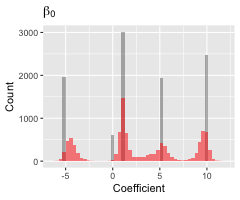
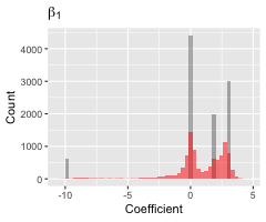
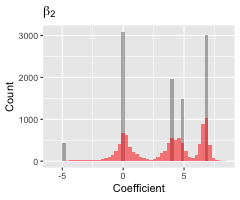
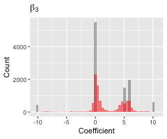
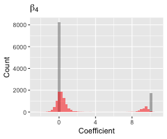
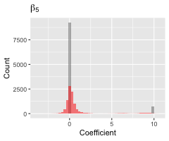
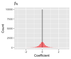
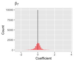
Figure 3: Histograms of distributions of fitted coefficient values. Color code: ground truth (grey) and tree boosted VCM (red).

4.2 Model Accuracy

To show the accuracy of our proposed methods, we have selected 12 real world datasets and run tree boosted VCM (marked as TVCM) against other benchmark methods. Table 1 demonstrates the results under classification settings with three benchmarks: GLM as logistic regression, GLM(S) as a partially saturated logistic regression model where each combination of discrete action covariates acts as fixed effect with its own level, and AdaBoost. Table 2 demonstrates the results under regression settings. The three benchmarks we choose here are: LM as linear model, LM(S) as a partially saturated linear model, and GBM as the gradient boosted trees. Although with additional structural assumptions, tree boosted VCM performs nearly on a par with both GBM and AdaBoost. It benefits from its capability of modeling the action space without structural conditions to outperform the fixed effect linear model in certain cases.

NAME	GLM	GLM(S)	ADABOOST	TVCM
MAGIC04	0.208(0.007)	0.209(0.0065)	0.13(0.0076)	0.209(0.0072)
BANK	0.111(0.0044)	0.1(0.0044)	0.098(0.0035)	0.114(0.0043)
OCCUPANCY	0.014(0.0042)	0.0129(0.0034)	0.00567(0.0016)	0.0126(0.0048)
SPAMBASE	0.0749(0.011)	0.0732(0.012)	0.0564(0.0098)	0.0616(0.0097)
ADULT	0.188(0.004)	0.155(0.0046)	0.136(0.0049)	0.154(0.0028)
EGRIDSTAB	0.289(0.014)	0.227(0.018)	0.179(0.009)	0.177(0.015)

Table 1: Prediction accuracy of classification and 0-1 loss for six UCI data sets through tenfold cross validation. Results are shown as mean(sd). Sources of some datasets are: BANK(Moro et al., 2014) and OCCUPANCY(Candanedo and Feldheim, 2016).

NAME	LM	LM(S)	GBM	TVCM
BEIJINGPM	6478(227)	5041(203)	3465(176)	3942(178)
BIKEHOUR	24590(1630)	12190(818)	5791(419)	6596(597)
STARCRAFT	1.135(0.0622)	1.116(0.0645)	1.045(0.0594)	1.161(0.0596)
ONLINENEWS	0.8544(0.0331)	0.8377(0.0328)	0.7826(0.0298)	0.8183(0.0337)
ENERGY	18.01(4.42)	9.801(2.16)	0.5633(0.162)	9.864(2.27)
EGRIDSTAB	1.01e-03(4.5e-05)	6.92e-04(3e-05)	4.31e-04(1.4e-05)	4.27e-04(8.3e-06)

Table 2: Prediction accuracy of regression and mean square error for six UCI data sets through tenfold cross validation. Results are shown as mean(sd). Sources of some datasets are: BEIJINGPM(Liang et al., 2015), BIKEHOUR(Fanaee-T and Gama, 2014), ONLINENEWS(Fernandes et al., 2015) and ENERGY(Tsanas and Xifara, 2012).

4.3 Visual Interpretability: Beijing Housing Price

Here we show the results of applying tree boosted VCM on the Beijing housing data (Kaggle, 2018). We take the housing unit price as the target regressed on covariates of location, floor, number of living rooms and bathrooms, whether the unit has an elevator and whether the unit has been refurbished. Specially, location has been treated as the action space represented in pairs of longitude and latitude. Location specific linear coefficients of other covariates are displayed in Figure 4. We allow 200 trees of depth of 5 in the ensemble with a constant learning rate of 0.05.

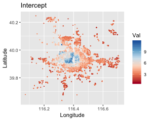
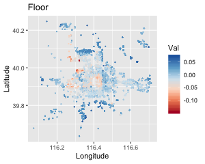
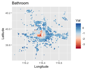
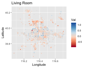
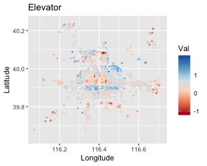
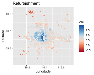
Figure 4: Beijing housing unit price broken down on several factors.

The urban landscape of Beijing is pictured by its old inner circle with a low skyline gradually transitioning to its modern outskirt rim of skyscrapers housing a young and new workforce. Our model intercept provides the baseline of the unit housing prices in each area. Despite their high values, most buildings inside the inner circle are old and not suitable for replanning, so elevators and number of bathrooms are of low contribution to the final price, while their refurbishment gets more attention. In contrast, outskirt housing gains more value if the unit has a complementary elevator and is on higher floor.

Figure 4 provides clear visualization of the fitted tree boosted VCM. Usually these irregular patterns are more likely to be outputs of nonparametric models, while behind each point on our plot is a location-specific linear model predicting the housing price breaking down to different factors.

4.4 Fitting Other Model Class

As mentioned, since VCM is the generalization of many specific models, our proposed fitting algorithm and analysis should apply to them as well. We take partially linear models as an example and consider the following data set from Cornell Lab of Ornithology consisting of the recorded observations of four species of vireos along with the location and surrounding terran types. We apply a tree boosted VCM under logistic regression setting using the longitude and the latitude as the action space and all rest covariates as linear effects, obtaining the model demonstrated by Table 3. The intercept plot suggests the trend of observed vireos favoring cold climate and inland environment, while the slopes of different territory types indicate a strong preference towards the low elevation between deciduous forests and evergreen needles.

Covariate	Slope	Covariate	Slope
Elevation	9.65e-04	Barren	-1.59e+03
Shallow Ocean	-1.88e+03	Evergreen Broad	2.77e+02
CoastShore Lines	-6.51e+01	Deciduous Needle	2.57e+02
Shallow Inland	9.39e+01	Deciduous Broad	2.72e+02
Moderate Ocean	-1.18e+03	Mixed Forest	7.32e+01
Deep Ocean	-5.12e+03	Closed Shrubland	-1.19e+03
Evergreen Needle	-4.54e+02	Open Shrubland	8.60e+01
Grasslands	-4.49e+02	Woody Savannas	-5.75e+02
Croplands	-4.29e+02	Savannas	-7.46e+02
Urban Built	-6.62e+02

Table 3: Fitting a partially linear model using tree boosted VCM. Plot on the left shows the nonparametric intercept. Table on the right shows the coefficients of predictive covariates.

5 Shrinkage, Selection and Serialization

Tree boosted VCM is compatible with any alternative boosting strategy in place of the boosting steps (B3) and (B4), such as the use of subsampled trees (Friedman, 2002; Zhou and Hooker, 2018), univariate or bivariate trees (Lou et al., 2012; Hothorn et al., 2013) or adaptive shrinkage (dropout) (Rashmi and Gilad-Bachrach, 2015; Rogozhnikov and Likhomanenko, 2017; Zhou and Hooker, 2018). While these alternative approaches have been empirically shown to help avoid overfitting or provide more model interpretability, we also anticipate that the corresponding varying coefficient mappings would inherit certain theoretical properties. For instance, Zhou and Hooker (2018) introduced a regularized boosting framework named Boulevard that guarantees finite sample convergence and asymptotic normality of its predictions. Incorporating Boulevard into our tree boosted VCM framework requires the changes to (B3) and (B4) such that

1. For each $j$, find a good fit $t_{b+1}^{j}\in\mathcal{T}:\mathbb{A}\to\mathbb{R}$ on $(z_{i},\Delta^{j}_{\beta_{i}})$ for $i\in w\subset\{1,\dots,n\}$ a random subsample.

2. Update $\hat{\beta}_{b}$ with learning rate $\lambda<1$.

   $$\hat{\beta}_{b+1}(\cdot)=\frac{b}{b+1}\hat{\beta}_{b}(\cdot)+\frac{\lambda}{b+1}\Gamma_{M}\left(\begin{bmatrix}t_{b+1}^{0}(\cdot)\\ \vdots\\ t_{b+1}^{p}(\cdot)\end{bmatrix}\right),$$

   where $\Gamma_{M}$ truncates the absolute value at some $M>0$.

By taking the same approach in the original paper, we can show that boosting VCM with Boulevard will also yield finite sample convergence to a fixed point.

Boulevard modifies the standard boosting strategy to the extent that new theoretical results have to be developed specifically. In contrast, there are other boosting variations that fall directly under the theoretical umbrella of tree boosted VCM. Our discussion so far assumes we run boosting iterations with a distinct tree built for each coefficient component while these trees are simultaneously constructed using the same batch of pseudo-residuals. Despite the possibility to utilize a single decision tree with multidimensional response to produce all components, as long as we build separate trees sequentially, the question arises that whether we should update the pseudo-residuals on the fly.

One advantage of doing so is the minimized boosting iteration from $(1+p)$ trees down to one tree, allowing us to use much larger learning rate $\lambda\leq 1/2$ instead of $\lambda\leq(1+p)^{-1}$ without changing the arguments we used to establish the consistency. We also anticipate that doing so in practice moderately reduces the cost as the gradients become more accurate for each tree. Here we will consider two approaches to conduct the on-the-fly updates.

In Hothorn et al. (2013) the authors proposed the component-wise linear least squares for boosting where they select which $\beta$ to update using the stepwise optimal strategy, i.e., choose $j_{b}$ and update $\beta^{j_{b}}$ if

$$j_{b}=\arg\min_{j=0,\dots,p}\sum_{i=1}^{n}l(y_{i},x_{i}^{T}(\hat{\beta}_{b}+\lambda t_{b}^{j}e_{j})(z_{i})),$$

the component tree that reduces the empirical risk the most. As a result, (B4) in Algorithm now updates

$$\hat{\beta}_{b+1}=\hat{\beta}_{b}+\lambda t_{b+1}^{j_{b}}e_{j_{b}}.$$

Notice that finding this optimum still requires the comparison among all components, therefore does not save any training cost when there are no better means or prior knowledge to help detect which component stands out. That being said, the optimal move is compatible with the key condition (C4) we posed to ensure consistency. Namely, it still guarantees that the population counterpart of boosting is efficient in reducing the gap between the estimate and the truth. However, this greedy strategy also complicates the pattern of the sequence in which $\beta$’s get updated.

Serialization refers to the cases when the $\beta$’s are being updated in some predetermined order. A similar model is covered by Lou et al. (2012, 2013) where the authors applied univariate generalized additive models (GAM) to perform model distillation, which was refined in Tan et al. (2017) using decision trees. Their models can either be built through backfitting which eventually produces one additive component for each covariate, or through boosting that generates a sequence of additive terms.

Applying the rotation of coordinates to tree boosted VCM, we can break each of the original boosting iterations into (p+1) micro steps to write

$$\hat{\beta}_{b,j}=\hat{\beta}_{b,j-1}-\lambda\nabla_{\beta^{j}}l(y,x^{T}\beta)\Big{|}_{\beta=\hat{\beta}_{b,j-1}(z)},$$

with j rotating through $0,\dots,p$. This procedure immediately updates the pseudo-residuals after each component tree is built. There are two feasible approaches if we intend to employ tree boosted VCM to achieve the same univariate GAM model. Either we can place all covariates into the action space and use only univariate decision trees to perform the serialized boosting, or we can directly apply tree boosted VCM to get additive models that are univariate with respect to the predictive covariates.

However, this procedure is not compatible with our consistency conclusion as the serialized boosting fails to guarantee (C4): each micro boosting step on a single coordinate relies on the current pseudo gradients instead of the gradients before the entire rotation. One solution is to consider an alternative to the determined updating sequence by randomly and uniformly proposing the coordinate to boost. In this regard,

$$\hat{\beta}_{b}=\hat{\beta}_{b}-\lambda\nabla_{\beta^{j}}l(y,x^{T}\beta)\Big{|}_{\beta=\hat{\beta_{b}}(z)},$$

where $j\sim\mbox{Unif}\{0,\dots,p\}$. This stochastic sequence solves the compatibility issue by satisfying (C4) with a probability bounded from below.

6 Conclusion

In this paper we studied the combination of gradient boosting and varying coefficient models. We introduced the algorithm of fitting tree boosted VCM under generalized linear model setting. We have proved the consistency of its coefficient estimators with an early stopping strategy. We have also demonstrated the performance of this method through diverse types of empirical studies. As a result we are confident to add gradient boosted decision trees into the collection of apt varying coefficient mappings.

We also discussed the model interpretability of tree boosted VCM, especially its parametric part as a self-explanatory component of reasoning about the covariates. Consistency guarantees the effectiveness of the interpretation. We also demonstrated a few visual aid for explaining tree boosted VCM.

There are a few future directions of this research. The performance of tree boosted VCM depends on boosting scheme as well as the component decision trees involved. It is worth analyzing the discrepancies between different approaches of building the boosting tree ensemble. Also, our discussions in the paper so far concentrate on the generic VCM. As mentioned, multiple regression and additive models can be considered as specifications of generic VCM, hence we expect model-specific conclusions and training algorithms.

Appendix A Proofs

A.1 Proof to Lemma 3.1

Proof.

$\xi_{n,6}$ is simply CLT. For the rest, we will conclude the corresponding function classes are $P-$Donsker. The collection of indicators for hyper rectangles $(-\infty,a_{1}]\times\dots,(-\infty,a_{p}]\subseteq\mathbb{R}^{p}$ is Donsker. By taking difference at most $p$ times we get all elements in $\mathcal{H}$, therefore $\mathcal{G}$, the indicators of $\mathcal{R}$, is Donsker. Thus $\xi_{n,1}=O_{p}\left(n^{-\frac{1}{2}}\right)$.

The basis functions $\mathcal{E}=\{1,x^{j},j=1,\dots,p\}$ is Donsker since all elements are monotonic and bounded since $x\in[-1,1]^{p}$. So $\mathcal{G}=\mathcal{H}\times\mathcal{E}$ is Donsker, which gives $\xi_{n,2}=O_{p}\left(n^{-\frac{1}{2}}\right)$ and $\xi_{n,4}=O_{p}\left(n^{-\frac{1}{2}}\right)$.

In addition, for fixed $f$, $f\mathcal{G}$ is therefore Donsker, which gives $\xi_{n,3}=O_{p}\left(n^{-\frac{1}{2}}\right)$. And $\mathcal{G}\times\mathcal{G}$ is Donsker, which gives $\xi_{n,5}=O_{p}\left(n^{-\frac{1}{2}}\right)$.

∎

A.2 Proof to Theorem 3.1

To supplement our discussion of norms, it is immediate that $\left\|g_{R,j}\right\|\leq\left\|h_{R}\right\|\leq 1.$ Another key relation is $\left\|g_{R,j}\right\|_{n,1}\leq\left\|h_{R}\right\|_{n,1}=\left\|h_{R}\right\|_{n}^{2}.$ We also assume that all $R$’s satisfy the terminal node condition.

Lemma A.1.

$\left\|\hat{r}_{b+1}\right\|_{n}\leq\left\|\hat{r}_{b}\right\|_{n}$, $\left\|r_{b+1}\right\|\leq\left\|r_{b}\right\|$.

Proof.

Consider the $p+1$ trees used for one boosting iteration with the terminal nodes denoted as $R^{j}_{i},0=1,\dots,p,i=1,\dots,m$, write $I_{R}=I\left(z\in R\right)$.

$$\left\|\hat{r}_{b+1}\right\|_{n} =\left\|\hat{r}_{b}-\lambda\sum_{j=0}^{p}\sum_{i=1}^{m}\frac{n^{-1}\left\langle\hat{r}_{b},g_{R^{j}_{i},j}\right\rangle_{n}}{n^{-1}\left\|h_{R^{j}_{i}}\right\|_{n}^{2}}g_{R^{j}_{i},j}\right\|_{n}$$

$$\leq\sum_{j=0}^{p}\left\|\sum_{i=1}^{m}\left(\lambda\hat{r}_{b}I_{R^{j}_{i}}-\frac{n^{-1}\left\langle\lambda\hat{r}_{b}I_{R^{j}_{i}},g_{R^{j}_{i},j}\right\rangle_{n}}{n^{-1}\left\|h_{R^{j}_{i}}\right\|_{n}^{2}}g_{R^{j}_{i},j}\right)\right\|_{n}$$

$$=\sum_{j=0}^{p}\left(\left\|\sum_{i=1}^{m}\left(\lambda\hat{r}_{b}I_{R^{j}_{i}}-\frac{n^{-1}\left\langle\lambda\hat{r}_{b}I_{R^{j}_{i}},g_{R^{j}_{i},j}\right\rangle_{n}}{n^{-1}\left\|h_{R^{j}_{i}}\right\|_{n}^{2}}g_{R^{j}_{i},j}\right)\right\|_{n}^{2}\right)^{\frac{1}{2}}$$

$$=\sum_{j=0}^{p}\left(\sum_{i=1}^{m}\left\|\lambda\hat{r}_{b}I_{R^{j}_{i}}-\frac{n^{-1}\left\langle\lambda\hat{r}_{b}I_{R^{j}_{i}},g_{R^{j}_{i},j}\right\rangle_{n}}{n^{-1}\left\|h_{R^{j}_{i}}\right\|_{n}^{2}}g_{R^{j}_{i},j}\right\|_{n}^{2}\right)^{\frac{1}{2}}$$

$$\leq\sum_{j=0}^{p}\left(\sum_{i=1}^{m}\left\|\lambda\hat{r}_{b}I_{R^{j}_{i}}\right\|_{n}^{2}\right)^{\frac{1}{2}}=\sum_{j=0}^{p}\left\|\lambda\hat{r}_{b}\right\|_{n}=\left\|\hat{r}_{b}\right\|_{n},$$

given $\left\|h_{R^{j}_{i}}\right\|_{n}^{2}\geq\left\|g_{R^{j}_{i},j}\right\|_{n}^{2}$. Same argument can be applied to the population version hence we get the second part.

∎

Lemma A.2.

For any $b\leq 0$, as defined in (7),

$$\sup_{x,z}|r_{b+1}(x,z)|\leq 2\sup_{x,z}|r_{b}(x,z)|.$$

Proof.

As implied by (6), for $(x,z)$ such that $z\in R$,

$$r_{b+1}(x,z)=r_{b}(x,z)-\lambda\sum_{i=0}^{p}\frac{\left\langle r_{b},g_{R,j}\right\rangle}{\left\|h_{R}\right\|^{2}}g_{R,j}(x,z).$$

The key observation is that

$$\left|\frac{\left\langle r_{b},g_{R,i}\right\rangle}{\left\|h_{R}\right\|^{2}}\right|=\left|\frac{\int r_{b}I\left(z\in R\right)x^{j}dP}{\int I\left(z\in R\right)^{2}dP}\right|\leq\sup_{x,z}|r_{b}(x,z)|.$$

Therefore, provided $|g_{R,i}|\leq 1$ and write $z\in R_{z}$,

$$\sup_{x,z}|r_{b+1}| \leq\sup_{x,z}|r_{b}|+\lambda\sup_{x,z}\sum_{i=0}^{p}\left|\frac{\left\langle r_{b},g_{R_{z},i}\right\rangle}{\left\|h_{R_{z}}\right\|^{2}}\right|\left|g_{R_{z},i}\right|$$

$$\leq\sup|r_{b}|+\lambda\sum_{i=0}^{p}\sup|r_{b}|\cdot 1$$

$$=2\sup_{x,z}|r_{b}|.$$

Recursively we can conclude that $\sup_{x,z}|r_{b}|\leq 2^{b}\sup_{x,z}|r_{0}|$. ∎

Lemma A.3.

Under conditions (C1)-(C6),

$$\left\|\hat{r}_{B}\right\|^{2}=\left\|r_{B}\right\|^{2}+\sigma_{\epsilon}^{2}+o_{p}\left(1\right),$$

where $\sigma^{2}_{\epsilon}=\left\|\epsilon\right\|^{2}$.

Proof.

Recall that

$$\hat{r}_{b+1}=\hat{r}_{b}-\lambda\sum_{j=0}^{p}\sum_{i=1}^{m}\frac{n^{-1}\left\langle\hat{r}_{b},g_{R^{j}_{i},j}\right\rangle_{n}}{n^{-1}\left\|h_{R^{j}_{i}}\right\|_{n}^{2}}g_{R^{j}_{i},j}=\hat{r}_{b}-\lambda\sum_{i=1}^{m(p+1)}\frac{n^{-1}\left\langle\hat{r}_{b},g_{b,i}\right\rangle_{n}}{n^{-1}\left\|h_{b,i}\right\|_{n}^{2}}g_{b,i},$$

and

$$r_{b+1}=r_{b}-\lambda\sum_{j=0}^{p}\sum_{i=1}^{m}\frac{\left\langle r_{b},g_{R^{j}_{i},j}\right\rangle}{\left\|h_{R^{j}_{i}}\right\|^{2}}g_{R^{j}_{i},j}=r_{b}-\lambda\sum_{i=1}^{m(p+1)}\frac{\left\langle r_{b},g_{b,i}\right\rangle}{\left\|h_{b,i}\right\|^{2}}g_{b,i}.$$

Therefore

$$\hat{r}_{b+1}-r_{b+1} =(\hat{r}_{b}-r_{b})+\lambda\sum_{j=0}^{p}\sum_{i=1}^{m}\left(\frac{\left\langle r_{b},g_{R^{j}_{i},j}\right\rangle}{\left\|h_{R^{j}_{i}}\right\|^{2}}-\frac{n^{-1}\left\langle\hat{r}_{b},g_{R^{j}_{i},j}\right\rangle_{n}}{n^{-1}\left\|h_{R^{j}_{i}}\right\|_{n}^{2}}\right)g_{R^{j}_{i},j}$$

$$=(\hat{r}_{b}-r_{b})+\lambda\sum_{i=1}^{m(p+1)}\left(\frac{\left\langle r_{b},g_{b,i}\right\rangle}{\left\|h_{b,i}\right\|^{2}}-\frac{n^{-1}\left\langle\hat{r}_{b},g_{b,i}\right\rangle_{n}}{n^{-1}\left\|h_{b,i}\right\|_{n}^{2}}\right)g_{b,i}$$

$$\triangleq(\hat{r}_{b}-r_{b})+\lambda\delta_{b}$$

$$=(\hat{r}_{0}-r_{0})+\lambda\sum_{j=0}^{b}\delta_{j}=\epsilon+\lambda\sum_{j=0}^{b}\delta_{j}.$$

Since for each fixed $j$, all $R_{i}^{j}$ are disjoint, we therefore define that

$$\gamma_{b}=\sum_{j=0}^{p}\sup_{i=1,\dots,m}\left|\frac{\left\langle r_{b},g_{R^{j}_{i},j}\right\rangle}{\left\|h_{R^{j}_{i}}\right\|^{2}}-\frac{n^{-1}\left\langle\hat{r}_{b},g_{R^{j}_{i},j}\right\rangle_{n}}{n^{-1}\left\|h_{R^{j}_{i}}\right\|_{n}^{2}}\right|,$$

which guarantees $\sup_{x,z}|\delta_{b}|\leq\gamma_{b}$. To bound $\gamma_{b}$, without loss of generality, we consider a single term involved such that

$$\frac{\left\langle r_{b},g_{b}\right\rangle}{\left\|h_{b}\right\|^{2}}-\frac{n^{-1}\left\langle\hat{r}_{b},g_{b}\right\rangle_{n}}{n^{-1}\left\|h_{b}\right\|_{n}^{2}} \triangleq\left(\frac{u}{v}-\frac{\hat{u}}{\hat{v}}\right)$$

$$=\left(\frac{u-\hat{u}}{v}+\left(\frac{1}{v}-\frac{1}{\hat{v}}\right)\hat{u}\right).$$

First consider

$$\hat{u}-u =\frac{1}{n}\left\langle\hat{r}_{b},g_{b}\right\rangle_{n}-\left\langle r_{b},g_{b}\right\rangle$$

$$=\frac{1}{n}\left\langle\epsilon+r_{b}+\sum_{j=0}^{b-1}\delta_{j},g_{b}\right\rangle_{n}-\left\langle r_{b},g_{b}\right\rangle$$

$$=\frac{1}{n}\left\langle\epsilon,g_{b}\right\rangle_{n}+\left(\frac{1}{n}\left\langle r_{b},g_{b}\right\rangle_{n}-\left\langle r_{b},g_{b}\right\rangle\right)+\left(\sum_{j=0}^{b-1}\frac{1}{n}\left\langle\delta_{j},g_{b}\right\rangle_{n}\right).$$

Per Lemma A.2, we have

$$\left|\frac{1}{n}\left\langle\epsilon,g_{b}\right\rangle_{n}\right|\leq\xi_{n}$$

and, by iteratively applying Lemma A.2 and setting $C_{0}=\max(\sup_{x,z}|f|,1),$

$$\left|\frac{1}{n}\left\langle r_{b},g_{b}\right\rangle_{n}-\left\langle r_{b},g_{b}\right\rangle\right|$$

$$= \left|\frac{1}{n}\left\langle f-\lambda\sum_{j=0}^{b-1}\sum_{i=1}^{m(p+1)}\frac{\left\langle r_{j},g_{j,i}\right\rangle}{\left\|h_{j,i}\right\|^{2}}g_{j,i},g_{b}\right\rangle_{n}-\left\langle f-\lambda\sum_{j=0}^{b-1}\sum_{i=1}^{m(p+1)}\frac{\left\langle r_{j},g_{j,i}\right\rangle}{\left\|h_{j,i}\right\|^{2}}g_{j,i},g_{b}\right\rangle\right|$$

$$\leq \left|\frac{1}{n}\left\langle f,g_{b}\right\rangle_{n}-\left\langle f,g_{b}\right\rangle\right|+\lambda\sum_{j=0}^{b-1}\sum_{i=1}^{m(p+1)}\left|\frac{1}{n}\left\langle\frac{\left\langle r_{j},g_{j,i}\right\rangle}{\left\|h_{j,i}\right\|^{2}}g_{j,i},g_{b}\right\rangle_{n}-\left\langle\frac{\left\langle r_{j},g_{j,i}\right\rangle}{\left\|h_{j,i}\right\|^{2}}g_{j,i},g_{b}\right\rangle\right|$$

$$\leq \left|\frac{1}{n}\left\langle f,g_{b}\right\rangle_{n}-\left\langle f,g_{b}\right\rangle\right|+\lambda\sum_{j=0}^{b-1}\sum_{i=1}^{m(p+1)}\left|\frac{\left\langle r_{j},g_{j,i}\right\rangle}{\left\|h_{j,i}\right\|^{2}}\right|\left|\frac{1}{n}\left\langle g_{j,i},g_{b}\right\rangle_{n}-\left\langle g_{j,i},g_{b}\right\rangle\right|$$

$$\leq \xi_{n}+\lambda\sum_{j=0}^{b-1}\sup|r_{j}|m(p+1)\xi_{n}$$

$$\leq \xi_{n}+C_{0}\sum_{j=0}^{b-1}2^{j}m\xi_{n}$$

$$\leq C_{0}2^{b}m\xi_{n}.$$

The last term could be bounded by

$$\left|\sum_{j=0}^{b-1}\frac{1}{n}\left\langle\delta_{j},g_{b}\right\rangle_{n}\right| \leq\frac{1}{n}\sum_{j=0}^{b-1}\left\|\delta_{j}\right\|_{n,\infty}\left\|g_{b}\right\|_{n,1}\leq\frac{1}{n}\sum_{j=0}^{b-1}\gamma_{j}\left\|h_{b}\right\|_{n}^{2},$$

where

$$\left\|g_{b}\right\|_{n,1}=\sum_{i=1}^{n}|g_{b}(x_{i})|,\quad\left\|\delta_{j}\right\|_{n,\infty}=\sup_{i=1,\dots,n}|\delta_{j}(x_{i})|.$$

Hence

$$|\hat{u}-u|\leq C_{0}2^{b}m\xi_{n}+\frac{1}{n}\sum_{j=0}^{b-1}\gamma_{j}\left\|h_{b}\right\|_{n}^{2}.$$

In order to bound $|\hat{u}|$, we notice

$$|\hat{u}|=\left|\frac{1}{n}\left\langle\hat{r}_{b},g_{b}\right\rangle_{n}\right| \leq\left(\frac{1}{n}\left\|\hat{r}_{n}\right\|_{n}^{2}\right)^{\frac{1}{2}}\cdot\left(\frac{1}{n}\left\|g_{b}\right\|_{n}^{2}\right)^{\frac{1}{2}}$$

$$\leq\left(\frac{1}{n}\left\|\hat{r}_{0}\right\|_{n}^{2}\right)^{\frac{1}{2}}\cdot\left(\frac{1}{n}\left\|g_{b}\right\|_{n}^{2}\right)^{\frac{1}{2}}$$

$$=\left(\frac{1}{n}\left\|f+\epsilon\right\|_{n}^{2}\right)^{\frac{1}{2}}\cdot\left(\frac{1}{n}\left\|g_{b}\right\|_{n}^{2}\right)^{\frac{1}{2}}$$

$$\leq(M+\sigma^{2}_{\epsilon}+\xi_{n})\cdot\left\|g_{b}\right\|$$

$$\leq(M_{0}+\xi_{n})\cdot\left\|h_{b}\right\|.$$

Therefore, we get an upper bound for

$$\left|\frac{\left\langle r_{b},g_{b}\right\rangle}{\left\|h_{b}\right\|^{2}}-\frac{n^{-1}\left\langle\hat{r}_{b},g_{b}\right\rangle_{n}}{n^{-1}\left\|h_{b}\right\|_{n}^{2}}\right| \leq\frac{|\hat{u}-u|}{|v|}+\left|\frac{1}{v}-\frac{1}{\hat{v}}\right||\hat{u}|$$

$$=\frac{C_{0}2^{b}m\xi_{n}+n^{-1}\sum_{j=0}^{b-1}\gamma_{j}\left\|h_{b}\right\|_{n}^{2}}{\left\|h_{b}\right\|^{2}}+\frac{\xi_{n}\cdot(M_{0}+\xi_{n})\cdot\left\|h_{b}\right\|}{\left\|h_{b}\right\|^{2}\cdot n^{-1}\left\|h_{b}\right\|_{n}^{2}}$$

$$\leq\frac{C_{0}2^{b}m\xi_{n}}{\left\|h_{b}\right\|^{2}}+\sum_{j=0}^{b-1}\gamma_{j}\left(1+\frac{\xi_{n}}{\left\|h_{b}\right\|^{2}}\right)+\frac{\xi_{n}(M_{0}+\xi_{n})}{\left\|h_{b}\right\|(\left\|h_{b}\right\|^{2}-\xi_{n})}.$$

Denote $h$ be the global minimum of the ensemble that $h=\min_{b,i,j}\left\|h_{R^{j}_{i}}\right\|$, since $m\leq(h^{2}-\xi_{n})^{-1}$, we obtain

$$\gamma_{b} \leq(p+1)\left(\frac{C_{0}2^{b}\xi_{n}}{h^{2}(h^{2}-\xi_{n})}+\sum_{j=0}^{b-1}\gamma_{j}\left(1+\frac{\xi_{n}}{h^{2}}\right)+\frac{\xi_{n}(M_{0}+\xi_{n})}{h(h^{2}-\xi_{n})}\right).$$

We would like to mention the elementary result that for a series $\{x_{n}\}$ satisfying

$$x_{n}\leq 2^{n}a+\sum_{i=0}^{n-1}bx_{i}+c,$$

the partial sums satisfy

$$\sum_{i=0}^{n}x_{n}\leq a\left(\frac{1-\left(\frac{2}{1+b}\right)^{n+1}}{1-\frac{2}{1+b}}\right)(1+b)^{n}-\frac{c}{b}.$$

Hence, we can verify this upper bound that

$$\sum_{j=0}^{B-1}\gamma_{j} \leq(1+p)^{B}\left(\frac{C_{0}}{h^{2}-\xi_{n}}\left(2+\frac{\xi_{n}}{h^{2}}\right)^{B}\left(1-\left(1-\frac{\frac{\xi_{n}}{h^{2}}}{2+\frac{\xi_{n}}{h^{2}}}\right)^{B-1}\right)-\frac{\xi_{n}(M_{0}+\xi_{n})}{h(h^{2}-\xi_{n})\left(1+\frac{\xi_{n}}{h^{2}}\right)}\right)$$

Recall the rates that $B=o(\log n),h^{2}=O_{p}\left(n^{-\frac{1}{4}+\eta}\right),\xi_{n}=O_{p}\left(n^{-\frac{1}{2}}\right)$, thus

$$\left(2+\frac{\xi_{n}}{h^{2}}\right)^{B}=2^{B}\cdot O_{p}\left(1\right),\quad 1-\left(1-\frac{\frac{\xi_{n}}{h^{2}}}{2+\frac{\xi_{n}}{h^{2}}}\right)^{B-1}=\frac{\xi_{n}}{h^{2}}\cdot O_{p}\left(1\right),$$

$$\frac{\xi_{n}(M_{0}+\xi_{n})}{h(h^{2}-\xi_{n})\left(1+\frac{\xi_{n}}{h^{2}}\right)}=\frac{\xi_{n}}{h^{3}}\cdot O_{p}\left(1\right).$$

Hence,

$$\sum_{j=0}^{B-1}\gamma_{j} \leq(1+p)^{B}\left(\frac{C_{0}}{h^{2}}\cdot 2^{B}\cdot\frac{\xi_{n}}{h^{2}}-\frac{\xi_{n}}{h^{3}}\right)O_{p}\left(1\right)=o_{p}(1),$$

which is equivalent to

$$\left\|\sum_{j=0}^{B-1}\delta_{j}\right\|\leq\sum_{j=0}^{B-1}\left\|\delta_{j}\right\|\leq\sum_{j=0}^{B-1}\gamma_{j}=o_{p}\left(1\right).$$

Combining all above we have

$$\left\|\hat{r}_{B}\right\|^{2} =\left\|r_{B}+\epsilon+\lambda\sum_{j=0}^{B-1}\delta{j}\right\|^{2}$$

$$\leq\left\|\epsilon\right\|^{2}+\left\|r_{B}\right\|^{2}+\lambda^{2}\left\|\sum_{j=0}^{B-1}\delta_{j}\right\|^{2}+2\lambda\left\|r_{B}+\epsilon\right\|\left\|\sum_{j=0}^{B-1}\delta_{j}\right\|$$

$$=\sigma_{\epsilon}^{2}+\left\|r_{B}\right\|^{2}+o_{p}\left(1\right).$$

∎

Lemma A.4.

Under condition (C1)-(C6), for any $\rho>0$ there exists $B_{0}=B_{0}(\rho)$ and $n_{0}=n_{0}(\rho)$ such that for all $n>n_{0}$,

$$P(\left\|r_{B_{0}}\right\|\leq\rho)\geq 1-\rho.$$

Proof.

Lemma 3 in Bühlmann (2002) proves this statement for rectangular indicators. By fixing $\lambda=(1+p)^{-1}$ and introducing conditions (C3) and (C4), formula (11) in Bühlmann (2002) still holds in terms of the single terminal node in each of the trees that corresponds to our defined $R^{*}$. Therefore cited Lemma 3 holds for our boosted trees. The conclusion is therefore reached by the assumption that $f\in\mbox{span}(\mathcal{G})$. ∎

Proof to main Theorem.

For a given $\rho>0$, since $\hat{r}_{B}(x^{*},z^{*})-f(x^{*},z^{*})$ is independent of $\epsilon$,

$$\mathbb{E}_{(x^{*},z^{*})}\left[{|\hat{\beta}_{B}(z^{*})^{T}x^{*}-f(x^{*},z^{*})|^{2}}\right] =\mathbb{E}_{(x^{*},z^{*})}\left[{|\hat{r}_{B}(x^{*},z^{*})-f(x^{*},z^{*})-\epsilon|^{2}}\right]-\left\|\epsilon\right\|^{2}$$

$$=\left\|\hat{r}_{B}\right\|^{2}-\left\|\epsilon\right\|^{2}$$

$$\leq\left\|r_{B}\right\|^{2}+o_{p}\left(1\right)$$

$$\leq\left\|r_{B_{0}}\right\|^{2}+o_{p}\left(1\right)$$

$$\leq\rho O_{p}\left(1\right)+o_{p}\left(1\right).$$

We reach the conclusion by sending $\rho\to 0$. ∎

A.3 Proof to Corollary 3.1.1

Proof.

We prove by contradiction. Assume there exists $0<\epsilon_{0}<s,c_{0}>0$ s.t.

$$P(\left\|\beta_{B}(z^{*})-\beta(z^{*})\right\|^{2}>\epsilon_{0})\geq c_{0}$$

for any sufficiently large $n$. Fix $n$ and consider any $z_{0}$ s.t. $\left\|\beta_{B}(z_{0})-\beta(z_{0})\right\|>\epsilon_{0}$. The corresponding open ball $B(x_{0},s)$ has volume $v_{0}=O(s^{p})$. Write $\beta=\begin{bmatrix}\beta^{0}\\ \beta^{-0}\end{bmatrix},$

$$\int_{B(x_{0},s)}\left\langle\begin{bmatrix}1\\ x\end{bmatrix},\beta_{B}(z_{0})-\beta(z_{0})\right\rangle^{2}dP_{x|z_{0}}$$

$$\geq c\int_{B(x_{0},s)}\left\langle\begin{bmatrix}1\\ x\end{bmatrix},\beta_{B}(z_{0})-\beta(z_{0})\right\rangle^{2}dx$$

$$\geq cv_{0}\left\langle\begin{bmatrix}1\\ x_{0}\end{bmatrix},\beta_{B}(z_{0})-\beta(z_{0})\right\rangle^{2}+c\int_{B(0,s)}\left\langle\begin{bmatrix}1\\ x\end{bmatrix},\beta_{B}(z_{0})-\beta(z_{0})\right\rangle^{2}dx$$

$$\geq cv_{0}(\beta_{B}(z_{0})^{0}-\beta(z_{0})^{0})^{2}+ct_{0}\left\|\beta_{B}(z_{0})^{-0}-\beta(z_{0})^{-0}\right\|^{2}$$

$$\geq c\min(v_{0},t_{0})\epsilon_{0}.$$

where $t_{0}=\int_{B(0,s)}x_{1}^{2}dx=O(s^{p}).$ That is equivalent to

$$\mathbb{E}_{(x^{*},z^{*})}\left[{|\hat{\beta}_{B}(z^{*})^{T}x^{*}-f(x^{*},z^{*})|^{2}}\right]>c\min(v_{0},t_{0})\epsilon_{0},$$

contradicting Theorem 3.1. ∎

References

• Basu et al. (2018) Basu, S., K. Kumbier, J. B. Brown, and B. Yu (2018). Iterative random forests to discover predictive and stable high-order interactions. Proceedings of the National Academy of Sciences, 201711236.
• Berger et al. (2017) Berger, M., G. Tutz, and M. Schmid (2017). Tree-structured modelling of varying coefficients. Statistics and Computing, 1–13.
• Breiman et al. (1984) Breiman, L., J. H. Friedman, R. A. Olshen, and C. J. Stone (1984). Classification and regression trees.
• Buergin and Ritschard (2017) Buergin, R. A. and G. Ritschard (2017). Coefficient-wise tree-based varying coefficient regression with vcrpart. Journal of Statistical Software 80(6), 1–33.
• Bühlmann (2002) Bühlmann, P. L. (2002). Consistency for l₂boosting and matching pursuit with trees and tree-type basis functions. In Research report/Seminar für Statistik, Eidgenössische Technische Hochschule (ETH), Volume 109. Seminar für Statistik, Eidgenössische Technische Hochschule (ETH).
• Candanedo and Feldheim (2016) Candanedo, L. M. and V. Feldheim (2016). Accurate occupancy detection of an office room from light, temperature, humidity and co2 measurements using statistical learning models. Energy and Buildings 112, 28–39.
• Chan and Loh (2004) Chan, K.-Y. and W.-Y. Loh (2004). Lotus: An algorithm for building accurate and comprehensible logistic regression trees. Journal of Computational and Graphical Statistics 13(4), 826–852.
• Chipman et al. (2016) Chipman, H. A., E. I. George, R. E. McCulloch, and T. S. Shively (2016). High-dimensional nonparametric monotone function estimation using bart. arXiv preprint arXiv:1612.01619.
• Fan et al. (2005) Fan, J., T. Huang, et al. (2005). Profile likelihood inferences on semiparametric varying-coefficient partially linear models. Bernoulli 11(6), 1031–1057.
• Fan et al. (1999) Fan, J., W. Zhang, et al. (1999). Statistical estimation in varying coefficient models. The annals of Statistics 27(5), 1491–1518.
• Fanaee-T and Gama (2014) Fanaee-T, H. and J. Gama (2014). Event labeling combining ensemble detectors and background knowledge. Progress in Artificial Intelligence 2(2-3), 113–127.
• Fernandes et al. (2015) Fernandes, K., P. Vinagre, and P. Cortez (2015). A proactive intelligent decision support system for predicting the popularity of online news. In Portuguese Conference on Artificial Intelligence, pp. 535–546. Springer.
• Friedberg et al. (2018) Friedberg, R., J. Tibshirani, S. Athey, and S. Wager (2018). Local linear forests. arXiv preprint arXiv:1807.11408.
• Friedman (2001) Friedman, J. H. (2001). Greedy function approximation: a gradient boosting machine. Annals of statistics, 1189–1232.
• Friedman (2002) Friedman, J. H. (2002). Stochastic gradient boosting. Computational Statistics & Data Analysis 38(4), 367–378.
• Gama (2004) Gama, J. (2004). Functional trees. Machine Learning 55(3), 219–250.
• Härdle et al. (2012) Härdle, W., H. Liang, and J. Gao (2012). Partially linear models. Springer Science & Business Media.
• Hastie and Tibshirani (1993) Hastie, T. and R. Tibshirani (1993). Varying-coefficient models. Journal of the Royal Statistical Society. Series B (Methodological), 757–796.
• Hothorn et al. (2013) Hothorn, T., P. Bühlmann, T. Kneib, M. Schmid, and B. Hofner (2013). mboost: Model-based boosting, 2012. URL http://CRAN. R-project. org/package= mboost. R package version, 2–1.
• Kaggle (2018) Kaggle (2018). Housing price in beijing. https://www.kaggle.com/ruiqurm/lianjia/home.
• Liang et al. (2015) Liang, X., T. Zou, B. Guo, S. Li, H. Zhang, S. Zhang, H. Huang, and S. X. Chen (2015). Assessing beijing’s pm2. 5 pollution: severity, weather impact, apec and winter heating. Proceedings of the Royal Society A: Mathematical, Physical and Engineering Sciences 471(2182), 20150257.
• Lou et al. (2012) Lou, Y., R. Caruana, and J. Gehrke (2012). Intelligible models for classification and regression. In Proceedings of the 18th ACM SIGKDD international conference on Knowledge discovery and data mining, pp.  150–158. ACM.
• Lou et al. (2013) Lou, Y., R. Caruana, J. Gehrke, and G. Hooker (2013). Accurate intelligible models with pairwise interactions. In Proceedings of the 19th ACM SIGKDD international conference on Knowledge discovery and data mining, pp.  623–631. ACM.
• Mallat and Zhang (1993) Mallat, S. and Z. Zhang (1993). Matching pursuit with time-frequency dictionaries. Technical report, Courant Institute of Mathematical Sciences New York United States.
• Melis and Jaakkola (2018) Melis, D. A. and T. Jaakkola (2018). Towards robust interpretability with self-explaining neural networks. In Advances in Neural Information Processing Systems, pp. 7786–7795.
• Mentch and Hooker (2016) Mentch, L. and G. Hooker (2016). Quantifying uncertainty in random forests via confidence intervals and hypothesis tests. The Journal of Machine Learning Research 17(1), 841–881.
• Moro et al. (2014) Moro, S., P. Cortez, and P. Rita (2014). A data-driven approach to predict the success of bank telemarketing. Decision Support Systems 62, 22–31.
• Park et al. (2015) Park, B. U., E. Mammen, Y. K. Lee, and E. R. Lee (2015). Varying coefficient regression models: a review and new developments. International Statistical Review 83(1), 36–64.
• Rashmi and Gilad-Bachrach (2015) Rashmi, K. and R. Gilad-Bachrach (2015). Dart: Dropouts meet multiple additive regression trees. In International Conference on Artificial Intelligence and Statistics, pp.  489–497.
• Ribeiro et al. (2016) Ribeiro, M. T., S. Singh, and C. Guestrin (2016). Why should i trust you?: Explaining the predictions of any classifier. In Proceedings of the 22nd ACM SIGKDD international conference on knowledge discovery and data mining, pp.  1135–1144. ACM.
• Rogozhnikov and Likhomanenko (2017) Rogozhnikov, A. and T. Likhomanenko (2017). Infiniteboost: building infinite ensembles with gradient descent. arXiv preprint arXiv:1706.01109.
• Scornet (2016) Scornet, E. (2016). Random forests and kernel methods. IEEE Transactions on Information Theory 62(3), 1485–1500.
• Tan et al. (2017) Tan, S., R. Caruana, G. Hooker, and Y. Lou (2017). Distill-and-compare: Auditing black-box models using transparent model distillation.
• Tsanas and Xifara (2012) Tsanas, A. and A. Xifara (2012). Accurate quantitative estimation of energy performance of residential buildings using statistical machine learning tools. Energy and Buildings 49, 560–567.
• van der Vaart and Wellner (1996) van der Vaart, A. W. and J. A. Wellner (1996). Weak convergence and empirical processes with applications to statistics. Springer.
• Wager and Athey (2018) Wager, S. and S. Athey (2018). Estimation and inference of heterogeneous treatment effects using random forests. Journal of the American Statistical Association 113(523), 1228–1242.
• Wang and Hastie (2014) Wang, J. C. and T. Hastie (2014). Boosted varying-coefficient regression models for product demand prediction. Journal of Computational and Graphical Statistics 23(2), 361–382.
• You et al. (2017) You, S., D. Ding, K. Canini, J. Pfeifer, and M. Gupta (2017). Deep lattice networks and partial monotonic functions. In Advances in Neural Information Processing Systems, pp. 2981–2989.
• Zhang and Zhu (2018) Zhang, Q.-s. and S.-C. Zhu (2018). Visual interpretability for deep learning: a survey. Frontiers of Information Technology & Electronic Engineering 19(1), 27–39.
• Zhou and Hooker (2018) Zhou, Y. and G. Hooker (2018). Boulevard: Regularized stochastic gradient boosted trees and their limiting distribution. arXiv preprint arXiv:1806.09762.