Dynamically optimal treatment allocation using Reinforcement Learning

Abstract.

Dynamic decisions are pivotal to economic policy making. We show how existing evidence from randomized control trials can be utilized to guide personalized decisions in challenging dynamic environments with constraints such as limited budget or queues. Recent developments in reinforcement learning make it possible to solve many realistically complex settings for the first time. We allow for restricted policy functions and prove that their regret decays at rate $n^{-0.5}$, the same as in the static case. We illustrate our methods with an application to job training. The approach scales to a wide range of important problems faced by policy makers.

Keywords. Policy learning, Reinforcement learning, Program evaluation

1. Introduction

Many important and challenging policy problems involve dynamic decision making. A healthcare system may need to manage queues in emergency situations or prioritize specific treatments under capacity constraints, an aid agency may want to distribute funds over time while facing borrowing constraints, a policy maker may need to assign job-training under limited budget to people who become unemployed sequentially. These settings are dynamic programming problems. A policy maker needs to make sequential decisions to maximize welfare, and her decisions affect future states (e.g. deplete a budget or increase queue length). If allocations in these problems could be improved, welfare gains for societies would be substantial. Yet, in real world applications, the number of potential state variables is often very large. A lot of information is available for individualizing decisions and should be taken into account. For instance, it is clearly beneficial for a medical administrator to induce different waiting times for patients with numerous different characteristics, symptoms, and medical histories.

This paper provides a framework for obtaining individualized treatment rules in dynamic settings. We describe both theoretical and computational tools for attacking these problems. Recent advances in reinforcement learning (RL) allow us to solve many realistically complicated decision problems for the first time. Like other methods, RL is a tool to obtain policy functions for dynamic programming problems. Yet, it can find policy functions for state spaces otherwise entirely out of reach (e.g., the policy function in Degrave et al (2022) has around 150 continuous state variables). As a result, RL has been the driving force behind many very prominent recent advances in artificial intelligence, e.g. mastering Go and Chess at previously unseen levels and without human knowledge, or controlling plasma in a nuclear fusion reactor (Silver et al, 2017; Silver et al, 2018; Degrave et al, 2022).

The contribution of the paper is twofold: (1) It is the first to show that it is possible to combine RL with RCT data to characterize optimal decisions in many highly relevant and challenging dynamic problems faced by economic policy makers. This has the potential to be a powerful aid. In addition, the combination of RL and causal inference developed in this paper is a deep necessity for the applications we consider. An important reason why RL breakthroughs so far have been seen in games, physical systems, or theoretical models is that in these environments the effects of a policy’s actions are known (e.g. through a physical model). We are able to expand the use of this technology into other real world domains only because tools from causal inference allow us to estimate the causal effect of the policy’s actions on its environment. In other words, we can only build our simulation to train an RL policy based on empirical data, because the RCT allows us to estimate the causal effect of the policy’s actions. (2) We provide the necessary theoretical support that our policy rule approaches the optimal welfare as the sample size of the RCT data grows (and approaches it relatively fast, which is important in practice). To obtain this, we study a suitable limiting version of the dynamic programming problem by following recent literature and taking the rate of arrivals to infinity (Wager and Xu, 2021; Fan and Glynn, 2021; Adusumilli, 2022), resulting in a continuous time approximation of the problem. Exploiting Partial Differential Equation (PDE) methods in a novel manner, we are able to prove that regret decays at a $n^{-1/2}$ rate, where $n$ is the sample size of the RCT. This is the same rate as in the setting without dynamics though it is not obvious a priori that the rate should continue to apply, since, under dynamics there is a great deal of dependence - the covariates of any individual affect the actions for all subsequently arriving individuals (e.g., by depleting the budget).

Our methodology is based on offline learning of the policy function (i.e., training the algorithm on existing data rather than experimenting live/online). There is a large and important literature on bandit algorithms for online learning, see e.g., Agarwal et al (2014), Russo and van Roy (2016), and Lattimore and Szepesvari (2021). This literature aims to learn the (heterogenous) treatment effects sequentially. However, our setup is different in that resource constraints evolve dynamically, e.g., the budget is depleted as more individuals are treated. These constraints do not affect the outcomes but constrain future actions, and standard bandit algorithms do not account for such variables. The focus of this paper is on devising algorithms that are dynamically optimal under resource constraints. To make headway on this problem we start with offline learning, though many of our insights extend to online learning as well (see Appendix E.2).

There are also good reasons why it is important to study offline learning in its own right. First, a large literature in RL has argued that sample efficient algorithms need to involve aspects of both online and offline learning, see e.g., Sutton and Barto (2018, Chapter 8), Yu et al, (2020) and Kidambi et al (2020). Online learning by itself is not welfare efficient; it would require prohibitively many rounds of experimentation to visit all states (e.g., all possible budgets) and it would not even be welfare optimal to do so. In our setting, the law of motion for state variables (i.e., how the budget changes) is known beforehand, so we can combine this with offline data to simulate dynamic environments. In fact, some of the best performing RL algorithms use techniques such as experience replay (Mnih et al, 2015), which is a form of offline learning. Second, online learning is not feasible if the outcomes are only known after a long gap (in our empirical example it is 3 years). Third, government agencies often need to be transparent about the rules being used and dynamically updating them in view of new data in real time might not be a realistic possibility. Finally, if subsequent online learning is desired to fine-tune the policy with newer data, our algorithm can be modified for this purpose as well. Still, a key feature of the approach is its ability to utilize large amounts of readily existing RCT data. If such RCT data already exists, at least initialising the training of policy parameters with it can reduce welfare costs of new experimentation.

With dynamic constraints being common across governmental and non-governmental settings, the following examples illustrate the generality of our approach:

Example 1.1.

(Finite budget) A social planner has received a one-off outlay of funds for providing treatment to individuals. Since the planner’s actions influence future states, in this case budget, this is a dynamic programming problem. The planner faces a trade-off in terms of using some of the funds to treat an individual immediately, or holding off until a more deserving individual arrives in the future. The future individuals’ utility is discounted. The planner would like a policy rule for treating individuals as a function of the individual covariates and current budget.

Two aspects of this example are worth highlighting: First, existing methods cannot be applied here even if the planner restricts consideration to stationary policy rules that are only a function of individual’s characteristics (by contrast, we call a policy non-stationary if it changes with budget or time). Techniques such as Empirical Welfare Maximization (EWM, Kitagawa and Tetenov, 2018), solve a simultaneous allocation problem where the policy rule is meant to be applied simultaneously on the population. Here, budget or capacity constraints are modeled as a constraint on the fraction of the population that can be treated. But in the present example, there is no set number to the population as individuals arrive sequentially, and hence no notion of a population fraction. Even more importantly, these methods cannot take into account the effect of discounting (see, Section 2.1 for a formal discussion). If the discount factor is small, it is optimal to wait for the people having the highest expected outcomes (based on their covariates) to turn up. If the discount factor is high, it would be optimal to treat anyone who is expected to benefit from the treatment. Discounting is an inherently dynamic consideration that has no counterpart in a fixed sample.

Second, stationary rules are inferior in terms of welfare to non-stationary rules that change with budget. When the budget is low, it is optimal to be more selective in treatment as opposed to when budget is high. A policy rule that changes continuously with budget can therefore deliver higher welfare. In an empirical illustration of this example in Section 6, we find that a non-stationary rule can deliver a welfare gain as high as 24% over a stationary one. Administratively, stationary rules are easier to communicate, so policy makers might favor stationary policies if the welfare loss is relatively small. Our method allows us to compute both and assess whether the additional welfare gain is worth having to justify the use of non-stationary rules which imply different policies at different points in time.

Example 1.2.

(Borrowing constraints) A social planner receives a steady flow of revenue, with individuals arriving at a constant rate. The planner is subject to a borrowing constraint. The optimal stationary policy maximizes welfare subject to the constraint that expected costs equal expected revenue. Under such a stationary policy, the budget would set off on a random walk, since the individuals are i.i.d. draws from a distribution, and the expected change to budget is 0 only on average. This implies the budget may accumulate to high levels, or hit the borrowing constraints over extended periods, both of which are sub-optimal. In fact, it is easy to verify that to achieve optimal welfare, the budget process needs to be controlled so it always takes on a constant value that is close to the borrowing constraint. Our methods enable us to solve for such a policy rule.

Example 1.3.

(Finite horizon) A planner receives an operating budget for each period, e.g. a year. Any unused funds will be sent back at the end of the year (this could be an approximation for how some governmental programs are run, with a budget outlay legislated at the beginning of each fiscal year). The planner would like to know the optimal policy rule for allocating treatments.

Example 1.4.

(Queues) Suppose the amount of time needed to treat an individual is longer than the average waiting time between the arrivals of two individuals. For instance, the treatment could be a medical procedure that takes time, or an unemployment service that requires the individual to meet with a caseworker. The social planner thus places the individuals selected for treatment in a queue. It is then useful to turn people away from treatment if the length of the queue is too long. Given some known or estimable cost of waiting, the planner would like to determine the optimal rule for whether or not to place an individual in a queue, as a function of the individual characteristics and the current waiting times. Generalizing the above, the planner may also want to allow for multiple queues, with the shorter queues reserved for individuals deemed more at risk.

In all these examples, we show how one can leverage RCT data to estimate the policy function that maximizes expected welfare. Beyond the issues highlighted above, our methods also allow for time varying rates of arrivals, time varying distributions of covariates, and uncertainty in arrival rates.

We discuss algorithms to minimize regret within a pre-specified policy class. As explained by Kitagawa and Tetenov (2018), one may wish to do this for ethical or legal reasons. Another reason is incentive compatibility - the planner may prefer a stationary policy (that depends only on covariates) to prevent manipulation of arrival times. For non-stationary policies, we assume the policy does not affect the arrival rates and the covariate distribution of individuals. This is reasonable in settings like unemployment, arrivals to emergency rooms etc., where the time of arrival is determined by factors exogenous to the provision of treatment.

In simple settings - see, e.g., Section 6 - the optimal policies can be estimated exactly (i.e., without numerical error) using PDE methods. But even with a moderate number of state variables, this quickly becomes infeasible. Hence, for computation, we utilise RL, namely an Actor-Critic (AC) algorithm (e.g., Sutton et al, 2000) with a parallel implementation - known as A3C (Mnih et al, 2016) - that can solve for the optimal policy within a pre-specified policy class. Our implementation of the algorithm is informed by our PDE theory, which enables us to achieve dimension reduction in the value function.

We illustrate the feasibility of our methodology using data from the Job Training Partnership Act (hereafter JTPA). We incorporate dynamic considerations into this setting in two ways: (1) a finite budget constraint as in Example 1.1; and (2) a finite budget and time constraint as in Example 1.3.

1.1. Literature review

If the dynamic aspect can be ignored, there exist a number of methods for estimating an optimal policy function that maximizes social welfare, starting from the seminal contribution of Manski (2004), and extended by Hirano and Porter (2009), Stoye (2009, 2012), Chamberlain (2011), Bhattacharya and Dupas (2012), and Tetenov (2012), among others. More recently, Kitagawa and Tetenov (2018), and Athey and Wager (2018) proposed and extended Empirical Welfare Maximization in this context.

Bandits with knapsacks (Slivkins, 2019; Chapter 10) are a variant of standard bandits with resource constraints. Example 1.1 falls into this category. Compared to knapsack algorithms, our methodology amounts to solving the full dynamic programming problem; Section 6 shows that this can be solved efficiently using PDE techniques. For this reason, we expect our techniques to deliver higher welfare, though a formal comparison is difficult as knapsack algorithms are devised for online learning. Other advantages of our approach include a more natural handling of continuous covariates, and the ability to optimize within a constrained policy class.

Dynamic Treatment Regimes (DTRs) are another related literature, see e.g., Laber et al (2014) for an overview. DTRs consist of a sequence of individualized treatment decisions. The data in these studies is a sequence of dynamic paths for each individual. By contrast, the dynamics in our setting are faced by the social planner, not the individual.

There is a vast literature on the computation of optimal policy functions. Previous work in economics has often used Monte-Carlo methods or non-stochastic grid-based methods such as generalized policy iteration (e.g., Benitez-Silva et al, 2000). The AC approach is conceptually related to Monte Carlo methods. However, it incorporates additional ingredients such as ‘bootstrapping’, stochastic gradients and parallelization, which translates to substantial computational gains. We also prefer AC methods over other RL algorithms such as Q-learning, as they are known to be more stable, and, importantly for us, can also solve for the optimal policy within a chosen functional class. AC has been one of the default methods of choice for RL applications in recent years. In our application, we use 12 continuous terms (five continuous covariates with various interactions) in the policy function. The dimensionality can be challenging with grid based approaches, but the RL algorithm reaches a solution with relative ease.

In making use of the knowledge of dynamics, our methods fall under the banner of model-based RL. Recent studies (Yu et al, 2020; Kidambi et al, 2020) have argued that model based methods greatly expand the sample efficiency and applicability of RL. Compared to these works, our methods are narrowly tailored to the specific setup studied here, but for this same reason are more efficient. For instance, in Example 1.1, our algorithm does not need to visit all budget values to learn the optimal policy. But generic model-based RL methods behave conservatively when not all the states are reached, and typically minimize only a lower bound to regret.

2. Setup

Consider a social planner who is faced with making treatment decisions for a sequence of individuals under different institutional constraints. The state variables are denoted by $s:=(x,z,t),$ where $x$ denotes the vector of individual covariates, $z$ is the institutional variable (e.g., current budget), and $t$ is time. For convenience, we take $z$ to be scalar for the rest of this paper.

The arrivals are determined by an inhomogeneous Poisson point process with parameter $\lambda(t)N$. Here, $N$ is a scale parameter that determines the rate at which individuals arrive, while $\lambda(t)$ itself is normalized via $\lambda(t_{0})=1$. Thus $\lambda(t)$ is the relative frequency of arrivals at time $t$ compared to that at time $t_{0}$. Following recent literature (Wager and Xu, 2021; Fan and Glynn, 2021; Adusumilli, 2022) we take $N\to\infty$ to end up with a PDE for characterizing welfare. Any approach to determine policy rules must use one or more forecasts (or estimates) of the arrival function $\lambda(t)$ and use this as optimally as possible. Therefore, for the most part of this paper, we take $\lambda(t)$ as given (density forecasts are also possible, and discussed in the appendix).

Based on the state $s$, the planner makes a decision on whether to provide a treatment ($a=1)$ or not $(a=0$). The decision is governed by the policy rule, $\pi$, that specifies the probability of choosing action $a$ given state $s$:

$$\pi(a|\cdot):\mathcal{S}\longrightarrow[0,1];\ a\in\{0,1\}.$$

The set of all policy classes under consideration is denoted by $\Pi$. The policies are indexed by some (possibly infinite dimensional) parameter $\theta\in\Theta$. We discuss policy classes in Section 2.3.

Once an action, $a$, has been chosen, the planner receives a felicity/instantaneous utility of $Y(a,z,t)/N$ that is equivalent to the potential outcome of the individual under action $a$ and state $(z,t)$. The felicities are divided by $N$ to rescale them to a ‘per-person’ quantity, which will be convenient when we take $N\to\infty$. The definition of $Y(\cdot)$ allows, e.g., the cost of treatment to vary with $(z,t)$. The covariates and the set of potential outcomes for each individual are assumed to be drawn from a joint distribution $F$ that is independent of $z,t$ (see, however, Appendix E.1 for extensions to time-varying $F$).

We focus on utilitarian social welfare criteria: the welfare from administering actions $\{a_{i}\}_{i=1}^{\infty}$, when a sequence of individuals with potential outcomes $\{Y_{i}(1,z_{i},t_{i}),Y_{i}(0,z_{i},t_{i})\}_{i=1}^{\infty}$ arrives at times $\{t_{i}\}_{i=1}^{\infty}$ into the future, is given by $N^{-1}\sum_{i=1}^{\infty}e^{-\beta t_{i}}(Y_{i}(a_{i},z_{i},t_{i})-Y_{i}(0,z_{i},t_{i}))$. Note that we always define welfare relative to not treating anyone. This is a convenient normalization that ensures the welfare is $0$ if the budget is $0$.

Define $r(s,a)=E[Y(a,z,t)|s]$, where the expectation is taken under the distribution $F$, as the (unscaled) ‘reward’, i.e., the expected felicity, for the social planner from choosing action $a$ for an individual when the state variable is $s$. Given our relative welfare criterion, it will be convenient to normalize $r(s,0)=0$, and set $r(s,1):=E[Y(1,z,t)-Y(0,z,t)|s]$.

Conditional on $(a,s)$, the evolution of $z$ to $z^{\prime}$ is governed by the ‘law of motion’:

$$z^{\prime}-z=G_{a}(s)/N,$$

where $G_{a}(\cdot);a\in\{0,1\}$ is a known function. For instance, in Example 1.1, if the cost the cost of treatment were $c$, we would have

(2.1) $$G_{a}(s)=-c\cdot\mathbb{I}\{a=1\ \cap\ z>0\}.$$

We can interpret $G_{a}(s)$ as the flow rate of $z$, when the flow is defined with respect to the number of arrivals $\int_{t_{0}}^{t}\lambda(w)dw$. This implies $\lambda(t)G_{a}(s)$ is the flow rate of $z$ over time. For instance, if the planner receives interest income at the rate $bz$, where $b$ is the saving/borrowing rate and $z$ is current endowment, then $G_{a}(s)=bz/\lambda(t)$.

Let $V_{\theta,N}(s)$ denote the value function at some state $s$ under policy $\pi_{\theta}(\cdot)$, defined as the expected social welfare from implementing this policy when the initial state is $s$. In the fixed $N$ setting, we can characterize this recursively as

(2.2) $$V_{\theta,N}(s)=\frac{r_{\theta}(s)\pi_{\theta}(1|s)}{N}+E_{\theta}\left[e^{-\beta(t^{\prime}-t)}V_{\theta,N}\left(s^{\prime}\right)|s\right],$$

where $s^{\prime}\equiv(x^{\prime},z^{\prime},t^{\prime})$ denotes the state variable for the next arrival immediately following $s$, and $E_{\theta}[\cdot|s]$ is the expectation jointly over (i) the new covariate $x^{\prime}\sim F$, (ii) the waiting time $t^{\prime}-t\sim\textrm{Exponential}(N\lambda(t))$, and (iii) the randomized policy $\pi_{\theta}(\cdot)$, which influences the value of $z^{\prime}$ via $z^{\prime}=z+G_{A}(s)/N;\ A\sim\textrm{Bernoulli}(\pi_{\theta}(s))$. Unfortunately, the dependence of $V_{\theta,N}(s)$ on $x$ makes it hard to characterize its properties (for one, $V_{\theta,N}(\cdot)$ does not have a stable limit as $N\to\infty$). Furthermore, the iid nature of arrivals implies $x^{\prime}$ is independent of $s$, so it would be convenient to integrate this out and achieve a dimension reduction for the value function. This motivates the integrated value function $h_{\theta,N}(z,t):=E_{x\sim F}[V_{\theta,N}(x,z,t)]$.

In the limit as $N\to\infty$, $h_{\theta,N}(z,t)$ converges to the solution of the PDE:

(2.3) $$\beta h_{\theta}(z,t)-\lambda(t)\bar{G}_{\theta}(z,t)\partial_{z}h_{\theta}(z,t)-\partial_{t}h_{\theta}(z,t)-\lambda(t)\bar{r}_{\theta}(z,t) =0\ \textrm{on }\mathcal{U},$$

where

$$\bar{r}_{\theta}(z,t) :=E_{x\sim F}[r(s,1)\pi_{\theta}(1|s)|z,t],\$$

$$\bar{G}_{\theta}(z,t) :=E_{x\sim F}\left[G_{1}(s)\pi_{\theta}(1|s)+G_{0}(s)\pi_{\theta}(0|s)|z,t\right],$$

and $\mathcal{U}$ is the domain of the PDE (more on this below). In particular, under some assumptions noted in Section 5 , we show that

(2.4) $$\sup_{(z,t),\theta\in\Theta}\left|h_{\theta,N}(z,t)-h_{\theta}(z,t)\right|\leq K\sqrt{\frac{1}{N}}.$$

for some $K<\infty$. Equation (2.4) is a direct consequence of Theorem 1, proved in a more general setting in Section 5.

PDE (2.3), and relatedly (2.4), is a key contribution of this paper. The terms, $\lambda(t)\bar{r}_{\theta}(z,t)$ and $\lambda(t)\bar{G}_{\theta}(z,t)$, are the average rewards and average change to $z$ under $\pi_{\theta}$ when the state variable is $(z,t)$. Now, $\lambda(t)\bar{r}_{\theta}(z,t)$ can be interpreted as expected flow reward, while $\lambda(t)\bar{G}_{\theta}(z,t)\partial_{z}h_{\theta}(z,t)+\partial_{t}h_{\theta}(z,t)$ can be interpreted as the total rate of change of $h_{\theta}(\cdot)$ with respect to time. PDE (2.3) then equates the flow value of welfare, $\beta h_{\theta}(z,t)$, to the sum of the flow rewards and rate of change of $h_{\theta}(z,t)$. Thus the PDE has an asset pricing interpretation if we think of $\beta$ as the natural interest rate.

Remarkably, PDE (2.3) characterizes $h_{\theta}(\cdot)$ in terms of only the the expected (given $z,t$) rate of change, $\lambda(t)\bar{G}_{\theta}(z,t),$ of $z$, so e.g., the variance of $\delta(z):=z^{\prime}-z$ does not matter for welfare. Now, it is only in the limit as $N\to\infty$ that the second and higher moments of $\delta(z)$ are not relevant. For fixed $N$, it can seen from (2.2) that the entire distribution of $\delta(z)$ matters as $V_{\theta}(s^{\prime})$ is generally nonlinear in $z^{\prime}$. This highlights the usefulness of the continuous time limit. Another convenient aspect of the PDE is that it depends only on the current state $s$, which enables us to abstract away from the time series dependence of $z$ (which in turn makes the rewards dependent). This property is useful for deriving regret bounds.

2.0.1. Large $N$ approximation

$N$ can be interpreted as the expected number of individuals arriving in a unit time period. In our empirical application, where arrivals consist of people who just became unemployed, we measure $t$ in years. Then, $N$ corresponds to the number of unemployed individuals per year, which is a large number. Hence, we expect PDE (2.3) to provide a very good approximation in this setting.

2.0.2. General arrival processes

While it is natural to model arrivals as an exponential process, this is not necessary. In fact, the randomness of the arrivals becomes irrelevant for the properties of $h_{\theta}(z,t)$ as $N\to\infty$. Let $\Delta_{t}$ denote the waiting time between arrivals when the last arrival was at time $t$. We require $\lim_{N\to\infty}\mathbb{E}[N\Delta_{t}]=\lambda(t)$ and $\lim_{N\to\infty}\textrm{Var}[N\Delta_{t}]=0$ at each $t$ (note that these are satisfied by the exponential distribution with parameter $\lambda(t)N$). Any arrival process that satisfies these conditions will lead to PDE 2.3.

2.0.3. Batching

In practice, the planner may want group arrivals into small batches and apply the same policy rule on each batch. Our methods can easily accommodate batching. Let $B$ denote the batch size. Then, PDE (2.3) continues to apply as long as $B/N\to 0$, so applying our proposed policy rules with such small batches delivers the same welfare as not using batching. We can also account for larger batch sizes, $B/N\to c\in(0,1)$, by using piece-wise constant policy rules. These are policy rules that only change at specific time intervals; see Section 6.1 for an example.

2.1. Informal derivation of PDE (2.3) in a simplified setting

Because of the importance of PDE (2.3), we provide an intuitive derivation of it in a simplified version of Example 1.1 (with a budget constraint) where $\lambda(t)=1$ is constant for all $t$, $r(s,a)$ is independent of $z,t$ and the budget evolves as $G_{a}(s)=-\mathbb{I}(a=1)$. In this setting, $t$ is no longer a state variable. We can represent$V_{\theta,N}(x,z)$ in recursive form as

$$V_{\theta,N}(x,z) =\frac{r(x,1)}{N}\pi_{\theta}(1|x,z)+\left(1-\frac{\beta}{N}\right)E_{x^{\prime}\sim F}\left[V_{\theta,N}\left(x^{\prime},z-\frac{1}{N}\right)\pi_{\theta}(1|x,z)+V_{\theta,N}(x^{\prime},z)\pi_{\theta}(0|x,z)\right]$$

$$\hfill\qquad\textrm{for }z\geq 1/N,$$

$$V_{\theta,N}(x,z) =0,\quad\textrm{otherwise}.$$

In deriving the above, we used $E[e^{-\beta\Delta t}]=1-\frac{\tilde{\beta}}{N}$, where $\tilde{\beta}=\beta+O(N^{-1})$, and replaced $\tilde{\beta}$ with $\beta$ to simplify notation. Define $\bar{\pi}_{\theta}(a|z)=E_{x\sim F}[\pi_{\theta}(a|x,z)]$ and $\bar{r}_{\theta}(z)=E_{x\sim F}\left[r(x,1)\pi_{\theta}(1|x,z)\right]$. Then, taking expectations with respect to $x\sim F$ on both sides of the recursion for $V_{\theta,N}(\cdot)$ gives

(2.5) $$h_{\theta,N}(z) =\frac{\bar{r}_{\theta}(z)}{N}+\left(1-\frac{\beta}{N}\right)\left\{h_{\theta,N}\left(z-\frac{1}{N}\right)\bar{\pi}_{\theta}(1|z)+h_{\theta,N}(z)\bar{\pi}_{\theta}(0|z)\right\};\ z\geq 1/N,$$

$$h_{\theta,N}(z) =0,\quad\textrm{otherwise}.$$

Now subtract $h_{\theta,N}(z)$ from both sides, take a second order Taylor expansion of $h_{\theta,N}(z-1/N)$, and multiply the entire expression by $N$ (the derivation is only for intuition, in reality, $h_{\theta}(\cdot)$ need not be twice differentiable). Then, in the limit as $N\to\infty$, we end up with the following Ordinary Differential Equation (ODE) for the evolution of $h_{\theta}(.)$:

(2.6) $$\beta h_{\theta}(z)=\bar{r}_{\theta}(z)-\bar{\pi}_{\theta}(1|z)\partial_{z}h_{\theta}(z),\qquad h_{\theta}(0)=0.$$

This is just a special case of PDE (2.3).

Suppose we restrict attention to stationary policies that do not change with $z$. Then, $\bar{\pi}_{\theta}(1|z)\equiv\bar{\pi}_{\theta},\bar{r}_{\theta}(z)\equiv\bar{r}_{\theta}$ and we can obtain an explicit solution to (2.6) as $h_{\theta}(z)=\beta^{-1}\bar{r}_{\theta}\left(1-e^{-\beta z/\bar{\pi}_{\theta}}\right).$ The optimal policy $\theta^{*}$ solves $\max_{\theta}h_{\theta}(z_{0})$, where $z_{0}$ is the initial budget. On the other hand, the EWM rule with budget constraints corresponds to the population problem: $\max_{\theta}\bar{r}_{\theta}\ \textrm{s.t.}\ \bar{\pi}_{\theta}\leq\alpha$ for some given $\alpha\in[0,1]$. Clearly the two optimization problems are not equivalent. One can of course solve the EWM problem for each $\alpha$ and choose the one that results in the best value for $h_{\theta}(z_{0})$, but this requires knowledge of $h_{\theta}(\cdot)$ provided in this paper (and this derivation is only applicable to stationary policies).

2.2. Boundary conditions

To complete the dynamic model, we need to specify a boundary condition for (2.3). As illustrated by the examples in section 1, our approach can be applied to various situations. Different situations require different boundary conditions. We consider the following possibilities, which arguably cover the majority of relevant applications:

Dirichlet boundary condition.

This includes boundary conditions of the form $h_{\theta}(\underline{z},t)=0\ \forall\ t$ (e.g., a budget constraint as in a simple version of Example 1.1), or $h_{\theta}(z,T)=0\ \forall\ z$ (e.g., a finite time constraint), or both (as in Example 1.3). Here, $\underline{z}$ and $T$ are known constants. Formally, $\mathcal{U}\equiv(\underline{z},\infty)\times[t_{0},T)$, and the boundary condition is specified as ($T=\infty$ or $\underline{z}=-\infty$ is allowed)

(2.7) $$h_{\theta}(z,t) =0\ \textrm{on }\Gamma\equiv\{\{\underline{z}\}\times[t_{0},T]\}\cup\{(\underline{z},\infty)\times\{T\}\}.$$

We emphasize that the above does not impose any restrictions on $\pi_{\theta}(\cdot)$. In general, $\lim_{z\to\text{$\underline{z}$}}\pi_{\theta}(1|x,z,t)\neq 0$. In fact, it might even be optimal to allow
$\lim_{z\to\text{$\underline{z}$}}\pi_{\theta}(1|x,z,t)=1$ to treat as many individuals as possible before the constraints are hit. Formally, the domain of $\pi_{\theta}(a|\cdot)$ is only the interior $\mathcal{U}$. As the program terminates when the boundary is reached, there may be an effective discontinuity in the planners’ actions before and after the boundary. However, this has no bearing on the continuity of $h_{\theta}(z,t)$.

Periodic boundary condition.

When the program continues indefinitely, $t$ is a relevant state variable only as it relates to some periodic quantity, e.g., seasonality. So, in this setting (as in a version of Example 1.1 where seasonality is also important), $\mathcal{U}\equiv\mathbb{R}\times\mathbb{R}$, and we impose the periodic boundary condition:

(2.8) $$h_{\theta}(z,t)=h_{\theta}(z,t+T_{p})\ \forall\ (z,t)\in\mathbb{R}\times\mathbb{R}.$$

Here, $T_{p}$ denotes the period length. This boundary condition can only be valid if $\lambda(t),\bar{G}_{\theta}(z,t),\bar{r}_{\theta}(z,t)$ are periodic in $t$ with period length $T_{p}$. This implies that $\pi_{\theta}$ should also be periodic.

Neumann boundary condition.

Consider a no-borrowing constraint (as in Example 1.2) at $z=\underline{z}$. Assume that the planner receives a flow of funds at the rate $\sigma(z,t)$ with respect to time, and the rate of interest is $b$. Then, at $z=\underline{z}$, the flow rate of change of $z$ is $\sigma(\underline{z},t)+b\underline{z}$ and flow rewards are 0 (since no individual can be treated). Hence, the evolution of $h_{\theta}(z,t)$ at $z=\underline{z}$ is governed by

(2.9) $$\beta h_{\theta}(z,t)-\{\sigma(z,t)+bz\}\partial_{z}h_{\theta}(z,t)-\partial_{t}h_{\theta}(z,t)=0,\quad\textrm{on }\{\underline{z}\}\times[t_{0},T).$$

Intuitively, one can imagine that the coefficients $\bar{G}_{\theta}(z,t),\bar{r}_{\theta}(z,t)$ of PDE (2.3) are discontinuous at $z=\underline{z}$ and this discontinuity is formulated as the boundary condition (2.9). Thus, boundary conditions of this form allow the dynamics at the boundary to be different from those in the interior. This can also be useful in examples with queues or capacity constraints (e.g., when the queue length is $0$, or the capacity is full). The following generalization of (2.9) accommodates all these examples: set $\mathcal{U}\equiv(\underline{z},\infty)\times[t_{0},T)$ and the boundary condition to be

(2.10) $$\beta h_{\theta}(z,t)-\bar{\sigma}_{\theta}(z,t)\partial_{z}h_{\theta}(z,t)-\partial_{t}h_{\theta}(z,t)-\bar{\eta}_{\theta}(z,t) =0,\quad\textrm{on }\{\underline{z}\}\times[t_{0},T),$$

$$h_{\theta}(z,T) =0,\quad\textrm{on }(\underline{z},\infty)\times\{T\}.$$

Here, $\bar{\sigma}_{\theta}(\underline{z},t)$ and $\bar{\eta}_{\theta}(\underline{z},t)$ are known functions. We require $\bar{\sigma}_{\theta}(\underline{z},t)>\delta>0$ for all $t$, to ensure $z$ cannot decrease after hitting the boundary.

2.3. Policy classes and optimal policies

For the theory, we consider a class $\Pi$ of policies indexed by some (possibly infinite dimensional) parameter $\theta\in\Theta$.

For computation using RL methods, however, we require $\pi_{\theta}(.)$ to be differentiable in $\theta$. This still allows for rich spaces of policy functions. The class of soft-max functions is convenient and also commonly used in RL (see Sutton and Barto, 2018). Let $f(x,z,t)$ denote a vector of functions of dimension $k$. The soft-max function takes the form

(2.11) $$\pi_{\theta}^{(\sigma)}(1|s)=\frac{\exp(\theta^{\intercal}f(s)/\sigma)}{1+\exp(\theta^{\intercal}f(s)/\sigma)}.$$

As currently written, $\theta$ would need to be normalized, e.g., by setting one of the coefficients to $1$. The term $\sigma$ is a ‘temperature’ parameter that is either determined beforehand, or computed along with $\theta$, in which case we could subsume it into $\theta$ and drop the normalization. For a fixed $\sigma$, we define the soft-max policy class as $\Pi_{\sigma}:=\{\pi_{\theta}^{(\sigma)}(\cdot|s):\theta\in\Theta\}$, where each element, $\theta$, of $\Theta$ is suitably normalized. As $\sigma\to 0$, this becomes equivalent to the class of Generalized Eligibility Scores (Kitagawa and Tetenov, 2018), which are of the form $\mathbb{I}\{\theta^{\intercal}f(s)>0\}$. More generally, the class $\{\pi_{\theta}^{(\sigma)}(1|s):\theta\in\Theta,\sigma\in\mathbb{R}^{+}\}$ can approximate any deterministic policy, including the first best policy rule (i.e., the one that maximizes $h_{\pi}(z_{0},t_{0})$ over all possible $\pi$), arbitrarily well, given a large enough dimension $k$. For even more expressive policies, this can be generalized, e.g., to multi-layer neural networks.

In using RL methods, we cannot directly work with deterministic rules, as they are not differentiable in $\theta$. In practice, however, we just let the algorithm choose both $(\theta,\sigma)$, i.e., we drop $\sigma$ and let the algorithm optimize over $\theta\in\mathbb{R}^{k}$. This will eventually lead us to a deterministic policy if that is indeed optimal.

Note that (2.3) defines a class of PDEs indexed by $\theta$, the solution to each is the integrated value function $h_{\theta}(z,t)$ from following $\pi_{\theta}$. The social planner’s objective is to choose $\theta^{*}$ that maximizes the forecast welfare at the initial values, $(z_{0},t_{0})$, of $(z,t)$:

(2.12) $$\theta^{*}=\operatorname*{arg\,max}_{\theta\in\Theta}h_{\theta}(z_{0},t_{0}).$$

3. Sample version of the planner’s problem

The unknown parameters in the social planner’s problem are $F$ and $r(s,a)$. We suppose that the social planner can leverage observational data to obtain estimates $F_{n}$ and $\hat{r}(s,a)$ of $F$ and $r(s,a)$. For the most part, we consider the setting where $r(s,a)\equiv r(x,a)$ i.e., the rewards do not depend on $z,t$. In such cases, we suppose that the planner has access to an observational study consisting of a random sample $\{Y_{i},W_{i},X_{i}\}_{i=1}^{n}$ of size $n$ denoting observed outcomes $(Y_{i}\equiv W_{i}Y_{i}(1)+(1-W_{i})Y_{i}(0))$, treatments $(W_{i})$, and covariates $(X_{i})$. This sample is drawn from some joint population distribution over $(Y_{i}(1),Y_{i}(0),W_{i},X_{i})$, assumed to satisfy ignorability, i.e., $(Y_{i}(0),Y_{i}(1))\perp\!\!\!\perp W_{i}|X_{i}$. We further assume that the joint distribution of $(Y_{i}(1),Y_{i}(0),X_{i})$ is given by $F$, introduced in the previous section, and for simplicity we denote the entire population distribution of $(Y_{i}(1),Y_{i}(0),W_{i},X_{i})$ by $F$ as well. The empirical distribution, $F_{n}$, of these observations is thus a good proxy for $F$. Let $\mu(x,w):=E[Y(w)|X=x]$ denote the conditional expectations for $w\in\{0,1\}$, and $p(x)=E[W|X=x]$, the propensity score. We recommend a doubly robust method to estimate $r(x,1)$ over $x\in\textrm{support}(F_{n})$, e.g.,

(3.1) $$\hat{r}(X_{i},1)=\hat{\mu}(X_{i},1)-\hat{\mu}(X_{i},0)+(2W_{i}-1)\frac{Y_{i}-\hat{\mu}(X_{i},W_{i})}{W_{i}\hat{p}(X_{i})+(1-W_{i})(1-\hat{p}(X_{i}))},$$

where $\hat{\mu}(x,w)$ and $\hat{p}(x)$ are non-parametric estimates of $\mu(x,w)$ and $p(x)$ respectively.

We can then plug-in the above quantities to obtain

$$\hat{r}_{\theta}(z,t) :=E_{x\sim F_{n}}[\hat{r}(s,1)\pi_{\theta}(1|x,z,t)],\ \textrm{and}$$

$$\hat{G}_{\theta}(z,t) :=E_{x\sim F_{n}}\left[G_{1}(x,z,t)\pi_{\theta}(1|x,z,t)+G_{0}(x,z,t)\pi_{\theta}(0|x,z,t)\right].$$

Based on the above we can construct the sample version of PDE (2.3) as

(3.2) $$\beta\hat{h}_{\theta}(z,t)-\lambda(t)\hat{G}_{\theta}(z,t)\partial_{z}\hat{h}_{\theta}(z,t)-\partial_{t}\hat{h}_{\theta}(z,t)-\lambda(t)\hat{r}_{\theta}(z,t) =0\ \textrm{on }\mathcal{U},$$

together with the corresponding sample versions of the boundary conditions (2.7), (2.8) or (2.10). In fact, for technical reasons, the existence of a unique solution to PDE (3.2) is not guaranteed without additional assumptions. For this reason, it is useful to think of PDE (3.2) as a heuristic device. In practice, we would always work with a discretized version of (3.2), described below, which does not suffer from existence issues.

We discretize the arrivals so that the law of motion for $z$ is given by (the ‘prime’ notation denotes one-step ahead quantities following the current one)

(3.3) $$z^{\prime}=\max\left\{z+b_{n}^{-1}G_{a}(x,z,t),\underline{z}\right\},$$

for some approximation factor $b_{n}$. Additionally, in the approximation scheme, the difference between arrival times is specified as

(3.4) $$t^{\prime}-t\sim\min\left\{\textrm{Exponential}(\lambda(t)b_{n}),T-t\right\},$$

with the censoring at $T$ used as a device to impose a finite horizon boundary condition. To simplify the notation, we allow $G_{a}(s)$ and $r(x,1)$ to be potentially discontinuous at $z=\underline{z}$ in case of the Neumann boundary condition, and thus avoid the need for the quantities $\bar{\sigma}_{\theta}(z,t)$ and $\bar{\eta}_{\theta}(z,t)$. The rest of environment is the same as before. For this discretized setup, define $\tilde{h}_{\theta}(z,t)$ as the integrated value function at the state $(z,t),$ when an individual happens to arrive at that state. This can be obtained as the fixed point to the following dynamic programming problem:

(3.5) $$\tilde{h}_{\theta}(z,t)=\begin{cases}\frac{\hat{r}_{\theta}(z,t)}{b_{n}}+E_{n,\theta}\left[e^{-\beta(t^{\prime}-t)}\tilde{h}_{\theta}\left(z^{\prime},t^{\prime}\right)|z,t\right]\\ 0\hfill\textrm{for }(z,t)\in\Gamma\quad\textrm{(Dirichlet only)}\end{cases},$$  where

$$E_{n,\theta}\left[e^{-\beta(t^{\prime}-t)}f\left(z^{\prime},t^{\prime}\right)|z,t\right] :=\int e^{-\beta\frac{\omega}{b_{n}}}E_{x\sim F_{n}}\left[f\left(\max\left\{z+\frac{G_{1}(x,t,z)}{b_{n}},\underline{z}\right\},t+\frac{\omega}{b_{n}}\right)\pi_{\theta}(1|x,z,t)\right.$$

$$\qquad\left.+f\left(\max\left\{z+\frac{G_{0}(x,t,z)}{b_{n}},\underline{z}\right\},t+\frac{\omega}{b_{n}}\right)\pi_{\theta}(0|x,z,t)\right]g_{\lambda(t)}(\omega)d\omega$$

for any function $f$, and $g_{\lambda(t)}(\omega)$ denotes the right censored exponential distribution with parameter $\lambda(t)$ and censoring at $\omega=b_{n}(T-t)$.

The usual contraction mapping argument ensures that $\tilde{h}_{\theta}$ always exists as long as $T<\infty$ or $\beta<1$. We can therefore use $\tilde{h}_{\theta}$ as the feasible sample counterpart of $h_{\theta}$, and solve the sample version of the social planner’s problem:

(3.6) $$\tilde{\theta}=\operatorname*{arg\,max}_{\theta\in\Theta}\tilde{h}_{\theta}(z_{0},t_{0}).$$

4. The actor-critic algorithm

This section discusses a RL algorithm to efficiently compute $\tilde{\theta}$ in (3.5). We focus on the Dirichlet boundary condition.

We use an Actor-Critic (AC) algorithm for our context, for a more extensive discussion of its baseline version see Sutton and Barto (2018). The algorithm runs multiple episodes, each of which are simulations of the ‘sample’ dynamic environment. At each state $s\equiv(x,z,t)$, the algorithm chooses an action $a\sim\textrm{Bernoulli}(\pi_{\theta}(1|s))$, where $\theta$ is the current policy parameter. This results in a reward of $\hat{r}(s,a)$, and an update to the new state $s^{\prime}\equiv(x^{\prime},z^{\prime},t^{\prime})$, where $x^{\prime}\sim F_{n}$, and $z^{\prime},t^{\prime}$ are obtained as in (3.3) and (3.4). Based on $s,a$ and $s^{\prime}$, the policy parameter is updated to a new value $\theta$. This process repeats until $(z,t)$ reaches the boundary of $\mathcal{U}$. Following this, the algorithm starts a new episode with the starting values $(z_{0},t_{0})$, and continues in this fashion indefinitely.

In detail, the AC algorithm employs gradient descent along the direction $\tilde{g}(\theta)\equiv\nabla_{\theta}[\tilde{h}_{\theta}(z_{0},t_{0})]$:

$$\theta\longleftarrow\theta+\alpha_{\theta}\tilde{g}(\theta),$$

where $\alpha_{\theta}$ is the learning rate. Denote by $\tilde{Q}_{\theta}(s,a),$ the action-value function

(4.1) $$\tilde{Q}_{\theta}(s,a):=\hat{r}_{n}(s,a)+E_{n,\theta}\left[e^{-\beta(t^{\prime}-t)}\tilde{h}_{\theta}(z^{\prime},t^{\prime})|s,a\right],$$

where $\hat{r}_{n}(s,a):=\hat{r}(s,a)/b_{n}$ and $E_{n,\theta}[\cdot]$ has been defined in (3.5). The Policy-Gradient theorem (Sutton et al, 2000) provides an expression for $\tilde{g}(\theta)$ as

(4.2) $$\tilde{g}(\theta)=E_{n,\theta}\left[e^{-\beta(t-t_{0})}\left(\tilde{Q}_{\theta}(s,a)-b(s)\right)\nabla_{\theta}\ln\pi_{\theta}(a|s)\right],$$

for a ‘baseline’, $b(.)$, that can be any function of $s$. Let $\dot{h}_{\theta}(z,t)$ denote some functional approximation for $\tilde{h}_{\theta}(z,t)$. We use $\dot{h}_{\theta}(z,t)$ as the baseline. In addition, we also employ this to approximate $\tilde{Q}_{\theta}(s,a)$ by replacing $\tilde{h}_{\theta}$ with $\dot{h}_{\theta}$ in equation (4.1):

$$\tilde{Q}_{\theta}(s,a)\approx\hat{r}_{n}(s,a)+E_{n,\theta}\left[e^{-\beta(t^{\prime}-t)}\dot{h}_{\theta}(z^{\prime},t^{\prime})|s,a\right].$$

The above enables us to obtain an approximation for $\tilde{g}(\theta)$ as

(4.3) $$\tilde{g}(\theta)\approx E_{n,\theta}\left[e^{-\beta(t-t_{0})}\delta_{n}(s,s^{\prime},a)\nabla_{\theta}\ln\pi_{\theta}(a|s)\right],$$

where $\delta_{n}(s,s^{\prime},a)$ is the Temporal-Difference (TD) error, defined as

$$\delta_{n}(s,s^{\prime},a):=\hat{r}_{n}(s,a)+\mathbb{I}\left\{(z^{\prime},t^{\prime})\in\mathcal{U}\right\}e^{-\beta(t^{\prime}-t)}\dot{h}_{\theta}(z^{\prime},t^{\prime})-\dot{h}_{\theta}(z,t).$$

We now describe the functional approximation for $\tilde{h}_{\theta}(z,t)$. Let $\phi_{z,t}=(\phi_{z,t}^{(j)},j=1,\dots,d_{\nu})$ denote a vector of basis functions of dimension $d_{\nu}$ over the space of $z,t$. We approximate $\tilde{h}_{\theta}(z,t)$ as $\dot{h}_{\theta}(z,t)\approx\phi_{z,t}^{\intercal}v$, where the value weights, $v$, are updated using Temporal-Difference learning (Sutton and Barto, 2018):

(4.4) $$\nu\longleftarrow\nu+\alpha_{v}E_{n,\theta}\left[\delta_{n}(s,s^{\prime},a)\phi_{z,t}\right],$$

for some value learning rate $\alpha_{v}$.

Using equations (4.3) and (4.4), we can construct Stochastic Gradient Descent (SGD) updates for $\theta,\nu$ as

(4.5) $$\theta \longleftarrow\theta+\alpha_{\theta}e^{-\beta(t-t_{0})}\delta_{n}(s,s^{\prime},a)\nabla_{\theta}\ln\pi_{\theta}(a|s),$$

(4.6) $$\nu \longleftarrow\nu+\alpha_{\nu}\delta_{n}(s,s^{\prime},a)\phi_{z,t},$$

by getting rid of the expectations in (4.3) and (4.4). These updates are applied at every decision point or in batches, using those values of $(s,a,s^{\prime})$ that come up as the algorithm chooses actions according to $\pi_{\theta}$. Importantly, the updates (4.5) and (4.6) can be applied simultaneously - instead of waiting for the value parameters to converge - by choosing the learning rates so that the speed of learning for $\nu$ is much faster than that for $\theta$. This is an example of two-timescale SGD.

The pseudo-code for the resulting procedure is presented in Algorithm 1 in the appendix. The algorithm can be shown to converge under suitable choices of learning rates, see, e.g., Bhatnagar et al, 2009, and Appendix C.1 (even if, admittedly, these theoretical rates are seldom used).

4.1. Parallel and batch updates

In practice, SGD updates are volatile and may take a long time to converge. We use two techniques for stabilizing SGD: Asynchronous parallel updates, resulting in the A3C algorithm (see, Mnih et al, 2016), and batch updates. Asynchronous updating involves running multiple versions of the dynamic environment in parallel processes, each of which independently and asynchronously updates the shared global parameters $\theta$ and $v$. Since at any given point in time, the parallel threads are at a different point in the dynamic environment, successive updates are decorrelated. Additionally, the algorithm is faster by dint of being run in parallel. In batch updating, the researcher chooses a batch size $B$ such that the parameter updates occur only after averaging over $B$ observations. This reduces the variance of the updates at the cost of slightly higher memory requirements. The pseudocode for the AC algorithm with both these modifications is provided in Appendix C.1.

4.2. Tuning parameters

We need to specify the basis functions for the value approximation and the learning rates. The choice of the dimension, $d_{\nu}$, of the basis functions is based on computational feasibility. From a statistical point of view the optimal choice of $d_{\nu}$ is infinity, since we would like to compute $\tilde{h}_{\theta}(z,t)$ exactly. For the basis functions, it will be efficient to incorporate prior knowledge about the environment. For instance, if the boundary condition is of the form $\tilde{h}_{\theta}(0,t)=0\ \forall\ t$, the basis functions could be chosen so that they are also $0$ when $z=0$.

For the value learning rate, a common rule of thumb is $\alpha_{\nu}\approx 0.1/E_{n,\theta}\left[\left\|\phi_{z,t}\right\|\right]$ (see, e.g., Sutton and Barto, 2018). The value of $\alpha_{\theta}$, however, requires experimentation, although we found learning to be stable across a relatively large range of $\alpha_{\theta}$ in our empirical example.

5. Statistical and numerical properties

We start by discussing the existence and uniqueness of PDE (2.3).

5.1. Existence and uniqueness of viscosity solutions

For semi-linear PDEs of the form (2.3), it is well known that a classical solution (i.e., a solution $h_{\theta}(z,t)$ that is continuously differentiable) does not exist. We instead employ the weak solution concept of a viscosity solution (Crandall and Lions, 1983). This is a common solution concept for equations of the HJB form; see Crandall et al (1992) for a user’s guide, and Achdou et al (2017) for a useful discussion. The following ensures existence of a unique, continuous viscosity solution to (2.3):

Assumption 1.

(i) $\bar{G}_{\theta}(z,t)$, $\bar{r}_{\theta}(z,t)$ are Lipschitz continuous uniformly over $\theta\in\Theta$.

(ii) $\lambda(t)$ is bounded, Lipschitz continuous, and bounded away from $0$.

(iii) There exists $M<\infty$ such that $|\bar{r}_{\theta}(z,t)|,|\bar{G}_{\theta}(z,t)|\leq M$ for all $\theta,z,t$.

(iv) $\bar{\sigma}_{\theta}(\underline{z},t),\bar{\eta}_{\theta}(\underline{z},t)$ are bounded and Lipschitz continuous in $t$ uniformly over $\theta\in\Theta$. Furthermore, there exists $\delta>0$ such that $\bar{\sigma}_{\theta}(\underline{z},t)\geq\delta$ for all $\theta,t$.

The sole role of Assumption 1(i) is to ensure $h_{\theta}(z,t)$ exists and is uniformly Lipschitz continuous. In so far as the latter goes, Assumption 1(i) can be relaxed in specific settings. For instance, depending on the boundary condition, we can allow $\bar{G}_{\theta}(z,t),\bar{r}_{\theta}(z,t)$ to be discontinuous in one of the arguments, see Appendix D.1. For ODE (2.6), just integrability of $\bar{r}_{\pi}(z),\bar{\pi}(1|z)$ is sufficient. We do not address the question of minimal sufficient conditions, but make do with Assumption 1(i) for simplicity. Appendix D.1 provides primitive conditions for verifying Assumption 1(i) under the soft-max policy class (2.11). Briefly, we require either $\sigma$ be bounded away from $0$, or at least one of the covariates be continuous. With purely discrete covariates and $\sigma\to 0$, $\bar{G}_{\theta}(z,t)$ and $\bar{r}_{\theta}(z,t)$ will typically be discontinuous, unless the policies depend only on $x$.

Note that $G_{a}(s)$ is discontinuous in $a$. But this does not affect the continuity of $\bar{G}_{\theta}(z,t)$ since $G_{1}(s)$ and $G_{0}(s)$ enter separately in the definition of $\bar{G}_{\theta}(z,t)$.

Assumption 1(ii) implies the arrival rates vary smoothly with $t$ and are bounded away from 0. Assumption 1(iii) is a mild requirement ensuring the expected rewards and changes to $z$ are bounded. Assumption 1(iv) provides regularity conditions for the Neumann boundary condition.

Lemma 1.

Suppose that Assumption 1 holds, and $\beta\geq 0$ for the periodic boundary condition. Then for each $\theta$, there exists a unique viscosity solution $h_{\theta}(z,t)$ to (2.3) under the boundary conditions (2.7), (2.8) or (2.10).

5.2. Assumptions for regret bounds

In addition to Assumption 1, we impose:

Assumption 2.

(i) There exists $M<\infty$ such that $|Y(a,z,t)|,|G_{a}(s)|\leq M\ \forall\ (a,s)$.

(ii) In the Dirichlet setting with $\underline{z}>-\infty$, there exists $\delta>0$ s.t $\bar{G}_{\theta}(z,t)<-\delta$.

(iii) (Complexity of the policy function space) The collection of functions

$$\mathcal{I}\equiv\left\{\pi_{\theta}(1|\cdot,z,t):(z,t)\in\bar{\mathcal{U}},\theta\in\Theta\right\}$$

indexed by $z,t$ and $\theta$, is a VC-subgraph class with finite VC index $v_{1}$. Furthermore, for each $a=0,1$, the collection of functions

$$\mathcal{G}_{a}\equiv\left\{\pi_{\theta}(a|\text{\^{A}\textperiodcentered},z,t)G_{a}(\text{\^{A}\textperiodcentered},z,t):(z,t)\in\mathcal{\bar{U}},\theta\in\Theta\right\}$$

is also a VC-subgraph class with finite VC index $v_{2}$. Let $v:=\max\{v_{1},v_{2}\}$.

Assumption 2(i) is a boundedness assumption, imposed mainly for ease of deriving the theoretical results (see, e.g., Kitagawa and Tetenov, 2018). In practice, it is virtually guaranteed that the changes to budget are smaller than some finite number.

Assumption 2(ii) is required only in the Dirichlet setting, and even here, only where the boundary condition is determined partly by $z$. In these settings, $z$ plays the role of time, so we need the coefficient, $\bar{G}_{\theta}(z,t)$, multiplying $\partial_{z}h_{\theta}$ in PDE (2.3) to be non-singular. Typically, we already have $\bar{G}_{\theta}(z,t)<0$ in such settings (e.g., the budget can only be depleted), so Assumption 2(ii) additionally requires $\bar{G}_{\theta}(z,t)$ to be strictly bounded away from $0$. This is a mild restriction: if there exist some people that benefit from treatment and $\beta>0$, it is a dominant strategy to always treat some fraction of the population.

The term $v$ in Assumption 2(iii) is a measure of the complexity of the policy class. Since the policy class is chosen by the policy maker, this only puts some mild restrictions on that choice. Often, $G_{a}(s)$ is independent of $x$, as in equation (2.1), in which case $v_{1}=v_{2}$. In calculating the VC dimension, we treat $z,t$ as an index to the functions $\pi_{\theta}(1|\cdot,z,t)$, similarly to $\theta$. This is intuitive, since how rapidly the policy rules change with budget is also a measure of their complexity.

The next set of assumptions relate to the properties of the observational data from which we estimate $\hat{r}(s,a)$, see Section 3 for the terminology. For now, we focus on the situation where $(z,t)$ do not affect the potential outcomes, see Appendix D.3 for extensions.

Assumption 3.

(i) $Y(a,z,t)\equiv Y(a)$.

(ii) $\{Y_{i}(1),Y_{i}(0),W_{i},X_{i}\}_{i=1}^{n}$ are an iid draw from the distribution $F$.

(iii) (Selection on observables) $(Y_{i}(1),Y_{i}(0))\perp\!\!\!\perp W_{i}|X_{i}$.

(iv) There exists $\kappa>0$ such that $p(x)\in[\kappa,1-\kappa]$ for all $x\in\textrm{support}(F)$.

Assumption 3(ii) assumes the observed data is representative of the population. Assumption 3(iii) requires the observational data to satisfy ignorability. Assumption 3(iv) ensures the propensity scores are bounded away from 0 and 1. All three are trivially satisfied for RCT data.

Under Assumptions 2 and 3, there exist many different estimates of the rewards, $\hat{r}(x,1)$, that are consistent for $r(x,1)$. In this paper, we use the doubly robust estimates given in (3.1). We assume that the estimates $\hat{\mu}(X_{i},w),\hat{p}(X_{i})$ of $\mu(X_{i},w),p(X_{i})$ are obtained through cross-fitting (see, Chernozhukov et al, 2018, or Athey and Wager, 2018 for a description). We choose some non-parametric procedures, $\tilde{\mu}(x,w),\tilde{p}(x)$ for estimating $\mu(x,w),p(x)$, and apply cross-fitting to weaken the assumptions required and reduce bias. We impose the following high-level conditions on $\tilde{\mu}(x,w),\tilde{p}(x)$:

Assumption 4.

(i) (Sup convergence) There exists $c>0$ such that, for $w\in\{0,1\}$,

$$\sup_{x}|\tilde{\mu}(x,w)-\mu(x,w)|=O_{p}(n^{-c}),\quad\sup_{x}|\tilde{p}(x)-p(x)|=O_{p}(n^{-c}).$$

(ii) ($L^{2}$ convergence) There exists some $\xi>1/2$ such that

$$E\left[\left|\tilde{\mu}(x,w)-\mu(x,w)\right|^{2}\right]\lesssim n^{-\xi},\qquad E\left[\left|\tilde{p}(x)-p(x)\right|^{2}\right]\lesssim n^{-\xi}.$$

Assumption 4 is taken from Athey and Wager (2018). The requirements imposed are weak and satisfied by almost all non-parametric procedures.

5.3. Regret bounds

Our main result is a probabilistic bound on the regret, $h_{\theta^{*}}(z_{0},t_{0})-h_{\tilde{\theta}}(z_{0},t_{0})$, from employing $\pi_{\tilde{\theta}}$ as the policy rule. This is obtained by bounding the maximal difference between the integrated value functions, i.e., $\sup_{(z,t)\in\bar{\mathcal{U}},\theta\in\Theta}|\tilde{h}{}_{\theta}(z,t)-h_{\theta}(z,t)|$. The latter suffices since (see, e.g., Kitagawa and Tetenov, 2018)

$$h_{\theta^{*}}(z_{0},t_{0})-h_{\tilde{\theta}}(z_{0},t_{0})\leq 2\sup_{(z,t)\in\bar{\mathcal{U}},\theta\in\Theta}|\tilde{h}{}_{\theta}(z,t)-h_{\theta}(z,t)|.$$

As computing $\tilde{\theta}$ requires choosing a ‘approximation’ factor $b_{n}$, we characterize the numerical error resulting from any sequence $b_{n}\to\infty$.

Theorem 1.

Suppose that Assumptions 1-4 hold and $\beta>0$. Then, with probability approaching one, there exists $K<\infty$ independent of $(\theta,z,t)$ such that

$$\sup_{(z,t)\in\bar{\mathcal{U}},\theta\in\Theta}\left|\tilde{h}_{\theta}(z,t)-h_{\theta}(z,t)\right|\leq K\left(\sqrt{\frac{v}{n}}+\sqrt{\frac{1}{b_{n}}}\right),$$

under the Dirichlet boundary condition (2.7). Furthermore, there exists $\beta_{0}>0$ that depends only on the upper bounds for $\lambda(t)$ and $\bar{G}_{\theta}(\cdot)$ such that the above also holds under the periodic boundary condition (2.8) as long as $\beta\geq\beta_{0}$.

The term $b_{n}^{-1/2}$ in Theorem 1 corresponds to the approximation error. Setting $b_{n}\propto n$ ensures this is of the same order as the statistical regret. Unfortunately, the theorem does not account for the computational error arising from the use of RL algorithms (but PDE methods, useful in simple cases, do provide exact solutions). In fact, we are not aware of any theoretical results on the rates of convergence of AC algorithms. Nevertheless, Theorem 1 remains useful for comparing policies. If the empirical welfare of the estimated policy, $\pi_{\tilde{\theta}}$, is higher that that of some other policy, $\pi_{\theta}$, we see that the regret from using $\pi_{\tilde{\theta}}$ over $\pi_{\theta}$ cannot be higher than a factor of $1/\sqrt{n}$.

The theorem requires $\beta$ to be sufficiently large in the periodic setting. This is a standard requirement under infinite horizons, see e.g., Crandall and Lions (1983).

5.3.1. Regret bounds with empirical PDE solutions

We conjecture Theorem 1 holds for the Neumann boundary condition as well, but were unable to prove this with our current techniques. The case of $\beta=0$ is also not covered by the theorem. For these remaining cases, we offer alternative results bounding the regret from using $\hat{\theta}$, obtained as

(5.1) $$\hat{\theta}=\operatorname*{arg\,max}_{\theta}\hat{h}_{\theta}(z_{0},t_{0}),$$

where $\hat{h}_{\theta}(z,t)$ is the solution to the empirical PDE (3.2). While estimation of $\hat{\theta}$ is not always feasible (though PDE methods can be employed in some simple cases), the bounds we obtain are useful as a baseline for the regret when there is no numerical error.

Existence of $\hat{h}_{\theta}(z,t)$ does not follow from Lemma 1. We need a comparison theorem (Crandall et al 1992), which will guarantee existence and uniqueness. A sufficient condition for this is: $G_{a}(x,z,t),\pi_{\theta}(x,z,t)$ are uniformly continuous in $(z,t)$ for each $(x,\theta)$. We will therefore assume this below. While certainly onerous - it precludes deterministic policies that vary with $(z,t)$ in the soft-max class (though any $\sigma>0$ is fine) - we believe more powerful comparison theorems can be devised that eliminate this requirement and leave this as an avenue for future research.

Theorem 2.

Suppose that Assumptions 1-4 hold and $G_{a}(x,z,t),\pi_{\theta}(x,z,t)$ are uniformly continuous in $(z,t)$ for each $(x,\theta)$. Then, with probability approaching one,

$$\sup_{(z,t)\in\bar{\mathcal{U}},\theta\in\Theta}\left|\hat{h}{}_{\theta}(z,t)-h_{\theta}(z,t)\right|\leq C\sqrt{\frac{v}{n}},$$

for the boundary conditions (2.7) , (2.10) and (2.8), the latter requiring $\beta\geq\beta_{0}$.

The theorem allows $\beta$ to be arbitrary, even negative, under Dirichlet and Neumann boundary conditions. The intuition behind Theorem 2 is that by Kitagawa and Tetenov (2018) and Athey and Wager (2018), the coefficients of the PDEs (2.3) and (3.2), i.e., the quantities $\bar{G}_{\theta}(z,t),\bar{r}_{\theta}(z,t)$ and $\hat{G}_{\theta}(z,t),\hat{r}_{\theta}(z,t)$, are uniformly close. This implies the solutions are uniformly close as well, which we verify using the theory of viscosity solutions. The $n^{-1/2}$ rate for the regret cannot be improved, since Kitagawa and Tetenov (2018) show that this rate is optimal in the static case.

6. Empirical application

Consider a policy maker who is charged with assigning job training to a stream of individuals arriving sequentially when they become unemployed. The policy maker would like to obtain a policy rule that maximizes expected social welfare under budget and/or time constraints. We use the popular dataset on randomized training provided under the JTPA to illustrate how RL algorithms allow us to obtain personalized policy rules for such dynamic decision problems when there are many state variables. This dataset was also previously used by Kitagawa and Tetenov (2018). During 18 months, applicants who contacted job centers after becoming unemployed were randomized to receive job training or not. We follow the sample selection strategy of Kitagawa and Tetenov (2018), resulting in 9223 observations. The data contains baseline information about the participants as well as their subsequent earnings for 30 months, with the latter being the outcome of interest. We illustrate our methods in two settings:

The first setting corresponds to Example 1.1, where budget is finite but there is no time constraint. As argued in the introduction and Section 2.1, static methods, i.e., methods devised for simultaneous allocation, are not applicable here; this is so even if we restrict attention to stationary policies. In fact, depending on the parameter values, non-stationary policies can substantially outperform stationary ones in terms of welfare. Admittedly, stationary policies are easier to implement for a policy maker; our results provide useful information on when this tradeoff could be worth-while. The setting is also simple enough that it is possible to solve the optimization problem exactly, using differential-equation techniques.

The second setting corresponds to Example 1.3, i.e., there is a constraint on both budget and time. As in the first example, static methods are not directly applicable - the optimization problem they solve does not correspond to maximizing the sample analogue of welfare in this setting, as the latter can only be characterized as the solution of a dynamic programming problem (because actions now affect future states via changes to budget). Nevertheless, one may wonder how different these objectives are in specific instances. We therefore compare the policy rules obtained from our approach with a budget-constrained EWM benchmark that (necessarily) ignores dynamics. Even when employing stationary policies within the same policy class (so a like-to-like comparison is possible), using our methods results in a 25% gain in welfare. This highlights the importance of treating the problem as a dynamic programming one, as opposed to approximating it with a simultaneous allocation problem, see Section 6.2.2 for a further explanation. Interestingly, we find in this setting that non-stationary policies do not provide any discernible welfare gain over stationary ones (atleast under our chosen parameter values). Again, this would not have been known a priori, so our methods can help the policy maker in deciding which to implement. The setting is also computationally more demanding and we use it to introduce our RL approach.

6.1. Budget constraints

The planner is endowed with an initial budget $z_{0}$, measured as the fraction of expected arrivals per year that can be treated. For each individual who arrives, the planner has to decide whether to offer job training or not. The decision may be based on remaining budget, and individual characteristics. For the latter, we use education, previous earnings, and age. Job training is free to the individual, but costly to the planner who must spend for the training from her budget.

To simplify matters, we assume that arrival rates are constant (our next setting relaxes this). We consider two policy classes: (A) a stationary one of the form $\pi_{\theta}(1|s)=\mathbb{I}\{\theta_{0}+\theta_{1}^{\intercal}x\geq 0\}$, and (B) a non-stationary one $\pi_{\theta}(1|s)=\mathbb{I}\{f_{0}(z)+f_{1}(z)^{\intercal}x\geq 0\}$, where the functions $f_{0},f_{1}$ are allowed to vary unrestrictedly with budget, $z$. A stationary policy is potentially more attractive as the policy rule does not change with budget, so there is no incentive for individuals to manipulate arrival times and it is also arguably easier to implement.

We obtain the reward estimates $\hat{r}(x,1)$ from a cross-fitted doubly robust procedure as in (3.1), where we use simple OLS to estimate the conditional means, $\mu(x,a)$, and the propensity score is $2/3$, as set by the RCT. The optimal stationary policy is then computed analytically using the procedure described in Section 2.1. The optimal non-stationary policy is computed by solving ODE (2.6) using the technique of ‘piece-wise constant policy approximations’, see Krylov (1999). This involves approximating $f_{0}(z)$ and $f_{1}(z)$ with piece-wise constant functions that stay constant within a set of grid points $\{0,\Delta z,2\Delta z,\dots,z_{0}\}$ for budget. The values of $f_{0}(z)$ and $f_{1}(z)$ within each grid can then be computed recursively by starting from $z=0$ and iteratively employing the technique described in Section 2.1 (the value function at the end of each step becomes the initial condition of ODE (2.6) for the next iteration). We can thus approximate the optimal $f_{0},f_{1}$ arbitrarily well by letting $\Delta z\to 0$. We take $\Delta z=1/5000$ (because some covariates are discrete, the resulting approximation error is essentially $0$). In fact, fixing $\Delta z$ to a specific value (even though we do not do this here) would make this a batched policy. The use of ODE techniques is possible due to the presence of a single state variable, $z$, in $h_{\theta}(\cdot)$. With additional state variables, the methodology quickly becomes infeasible and we have to resort to RL algorithms.

Figures 6.1 and 6.2 illustrate how the optimal policy functions’ coefficients change with different amounts of available budget, and what this implies for the probability of treatment after averaging across the covariates. We use a discount factor of $\beta=-\ln(0.9)$ for the figures (i.e., rewards accruing after 1 year are multiplied by $0.9)$. Due to the discrete nature of some covariates, the coefficients are constant over some intervals of the budget. The optimal stationary policy varies under different initial endowments $z_{0}$, but always treats a smaller share of arrivals at any given budget value as compared to the non-stationary policy. It is inferior as it must remain constant even as the budget is used up over time. As figure 6.2 shows, the welfare gain from the non-stationary policy can be as high as 24%. For some budgets and discount factors, the difference is only moderate though. A policy maker with a desire for stationary rules might be willing to bear this welfare cost.

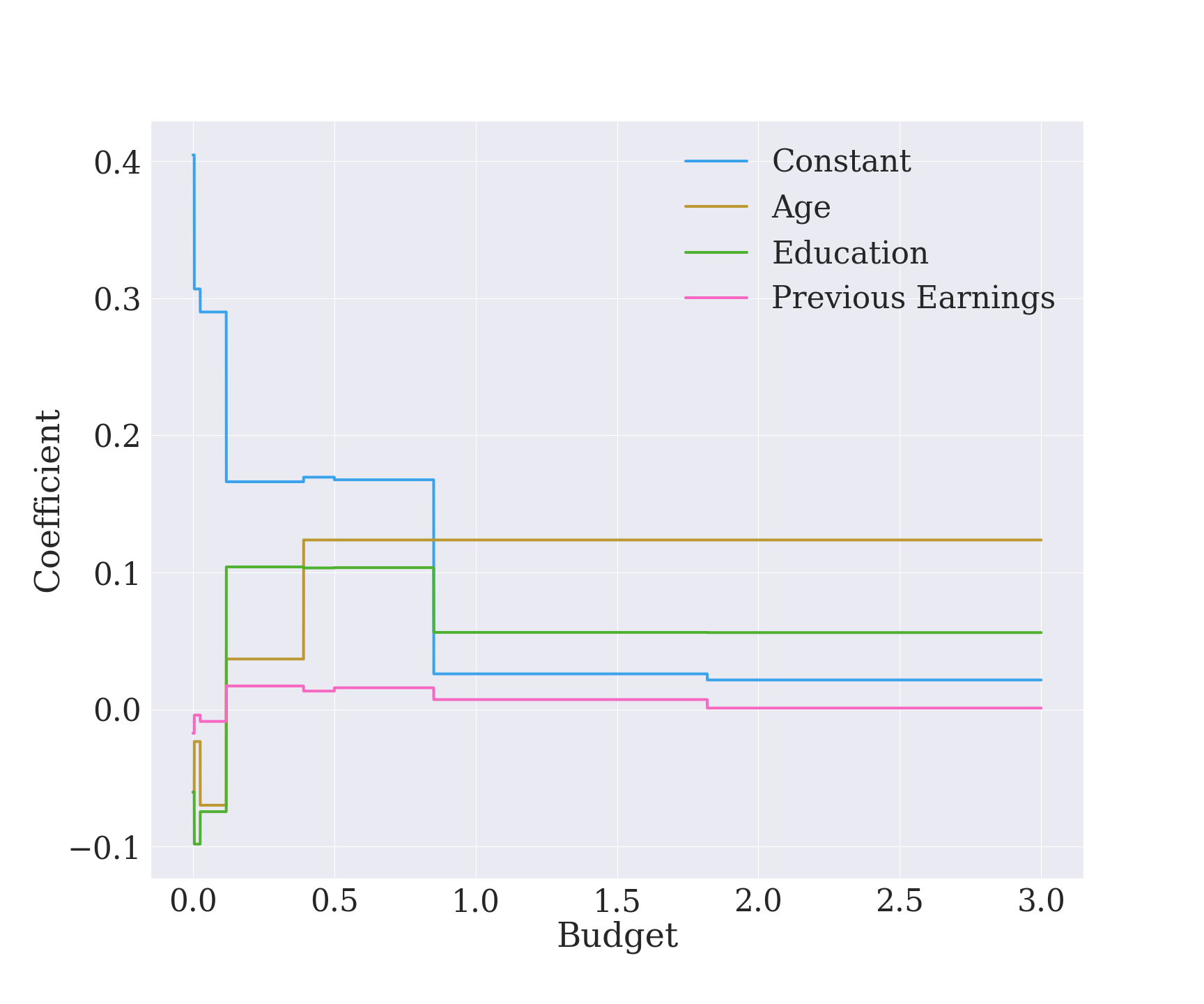
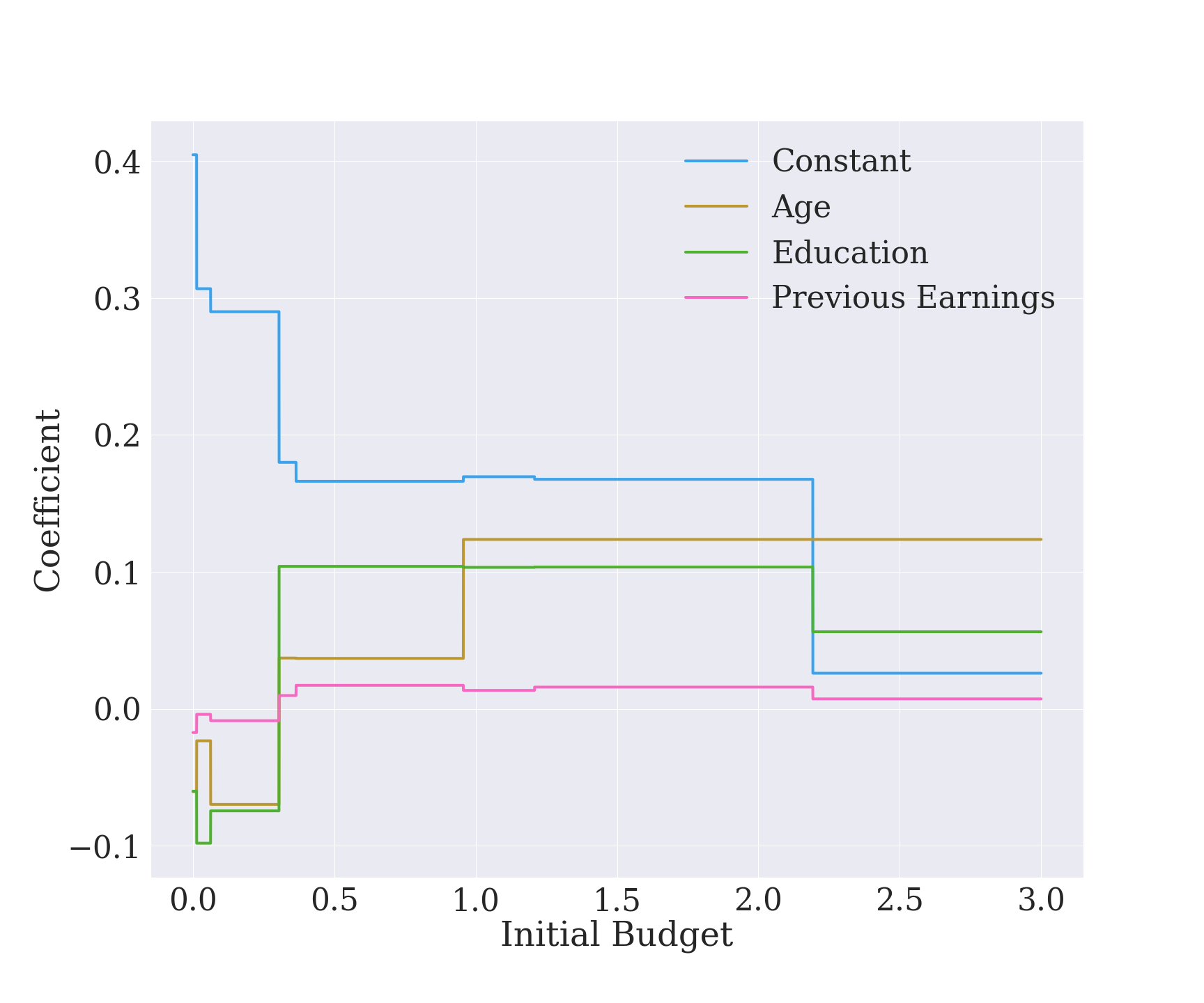
A: Non-Stationary Policy

B: Stationary Policy

Note: A budget of 1 corresponds to the expected cost of treating all arrivals of one year. The stationary policy is only affected by initial budget. The non-stationary policy responds to the remaining budget both at the initial value and over the course of its use.

Figure 6.1. Effect of Budget on Policies

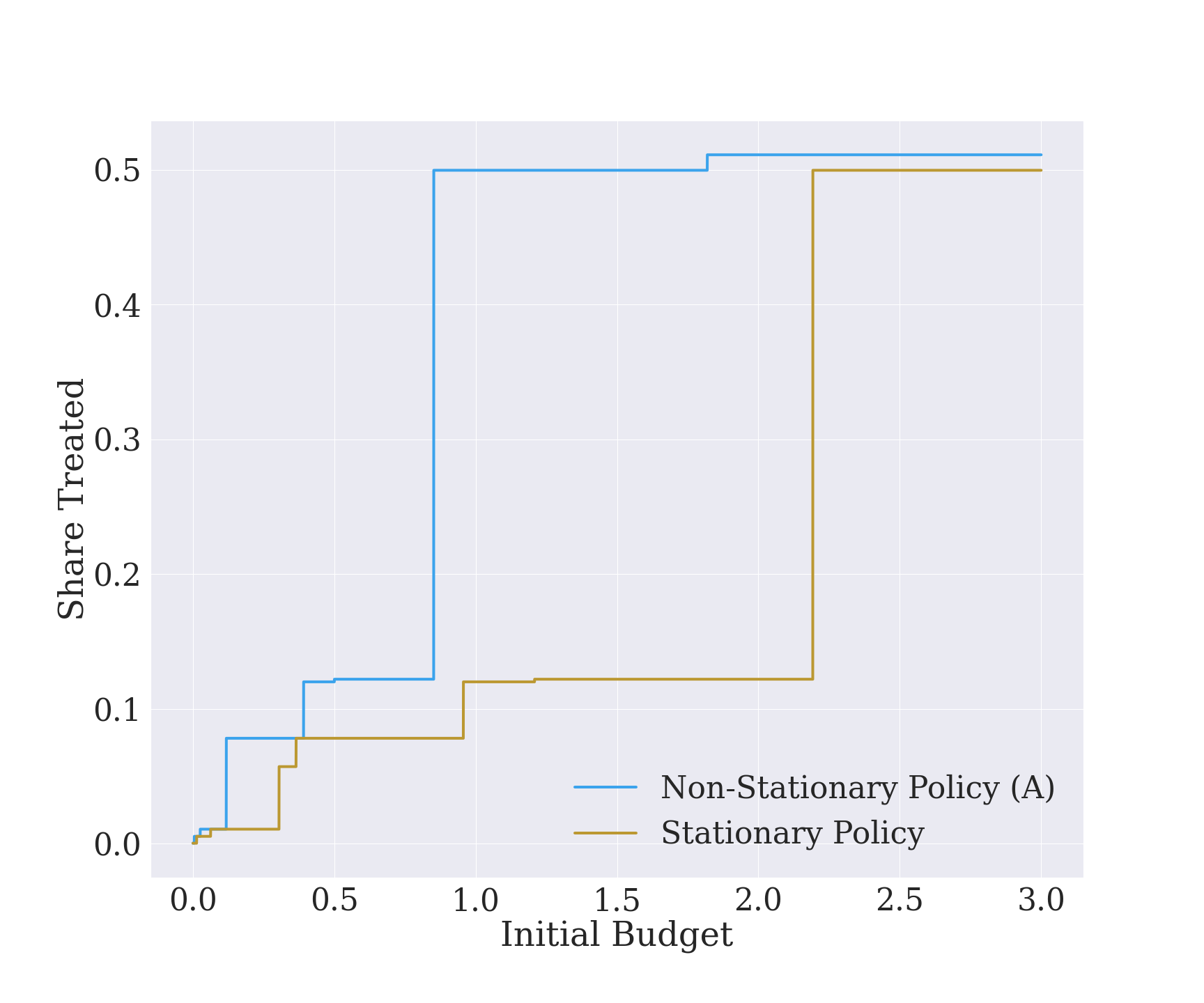
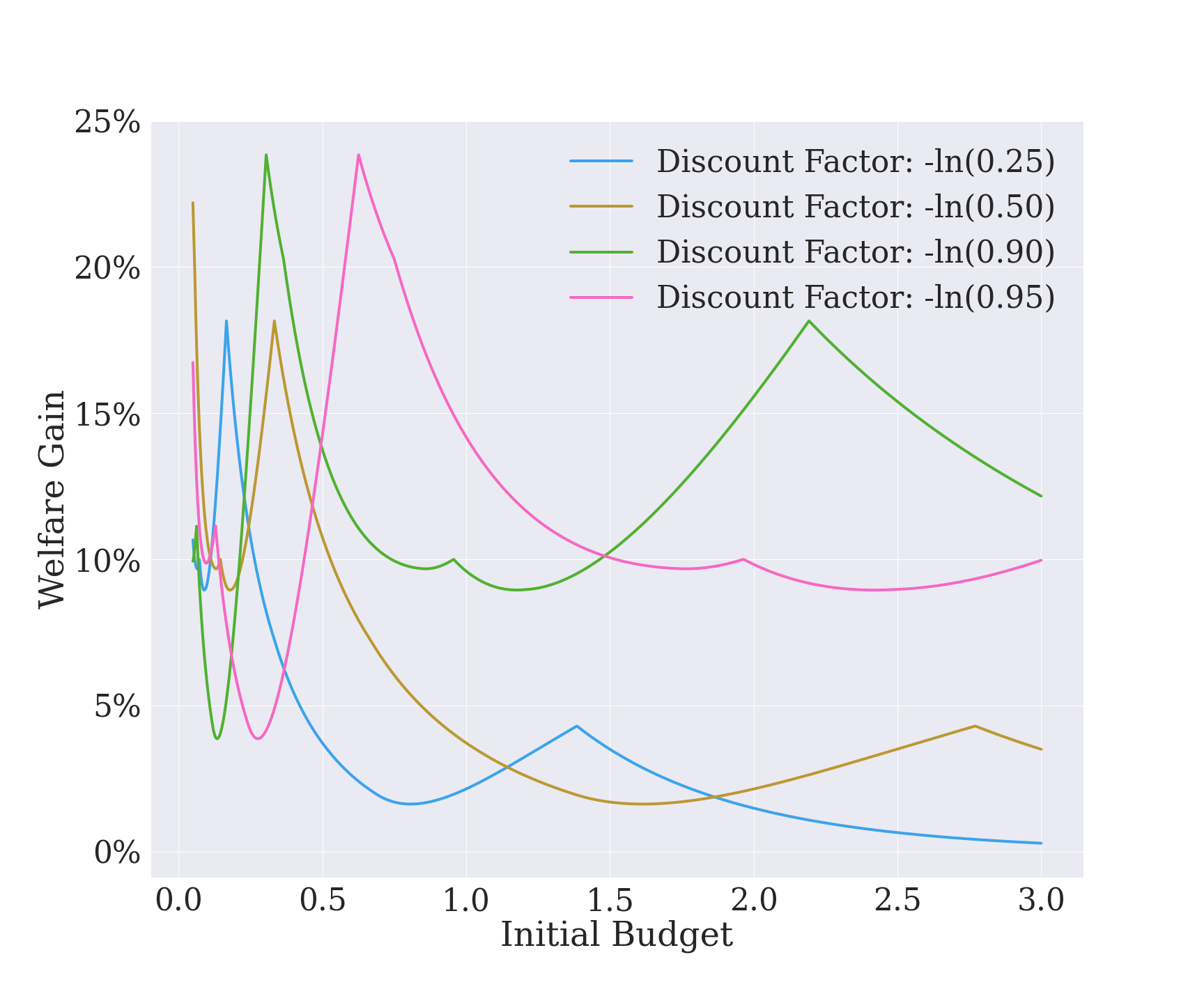
Note: A budget of 1 corresponds to the expected cost of treating all arrivals of one year. The share treated remains constant between an initial budget of 3 and 10. If not indicated otherwise, we use a discount factor of $-\log(0.9)$.

Figure 6.2. Effects of the Initial Budget

6.2. Budget and time constraints

We now consider a setting where the policy duration is $1$ year, and the planner is assumed to be endowed with a budget that can treat 25% of the expected number of arrivals per year. The program terminates when either all budget is used up or the year ends. The discount factor is $\beta=-\ln(0.9)$. We also allow the distribution of the arrivals to vary throughout the year. As the dataset contains information regarding when participants arrived, we can approximate the arrival process using cluster-specific inhomogeneous Poisson processes. We partition the data into four clusters using k-median clustering on the covariates, and estimate the arrival rates using Poisson regression. The procedure is described in Appendix F.

To apply our methods, we rescale time and budget so that $t=1$ corresponds to a year and set the initial budget, $z_{0}$, to 1. The cost of treatment is $c=4/5309$, where $5309$ is the expected number of people arriving in a year, given our Poisson rates. The reward estimates, $\hat{r}(x,1)$, are constructed in the same manner as in the previous example. We consider three policy classes: (A) a non-stationary policy: $\log(\pi_{\theta}(1|s)/(1-\pi_{\theta}(1|s))=\theta_{0}+\theta_{1}^{\intercal}{\bf x}+\theta_{2}^{\intercal}{\bf x}\cdot z+\theta_{3}^{\intercal}{\bf x}\cdot\cos(2\pi t)$, (B) a second non-stationary policy: $\log(\pi_{\theta}(1|s)/(1-\pi_{\theta}(1|s))=\theta_{0}+\theta_{1}^{\intercal}{\bf x}+\theta_{2}^{\intercal}{\bf x}\cdot z+\theta_{3}^{\intercal}{\bf x}\cdot D_{t}$ where $D_{t}$ are dummies for quarter of the year; and (C) a stationary one: $\log(\pi_{\theta}(1|s)/(1-\pi_{\theta}(1|s))=\theta_{0}+\theta_{1}^{\intercal}{\bf x}$, where ${\bf x}=(1,\textrm{age, education, previous earnings)}$. The rationale for using the $\cos(2\pi t)$ term was to account for the seasonal nature of arrivals. Policy classes A and B give almost identical outcomes (the difference in welfare is less than 0.5%). For brevity, we only display the outcomes from policy class A.

6.2.1. Tuning parameter choice

We solve for the optimal policies within each policy class using the A3C algorithm with clusters (see Appendix C.1). For the tuning parameters, we conducted a grid search with three different values for each of $\alpha_{\theta}\in\{0.5,5,50\}$, $\alpha_{v}\in\{10^{-3},10^{-2},10^{-1}\}$, and $d_{v}\in\{9,11,13\}$, where $d_{v}$ is the dimension of basis functions for the value approximation (see Appendix F for further details). Our implementation further has $20$ RL agents training in parallel (higher is better, this is only restricted by hardware constraints), with the batch size set to $B=1024$ (higher is better, but it appears there is little gain beyond a certain level). From the grid search we found that setting $\alpha_{\theta}=5$, $\alpha_{\nu}=10^{-2}$ and $d_{v}=9$ achieves reasonably quick and stable convergence (this is consistent with the rule of thumb choice for the value learning rate, which is $\alpha_{v}\approx 10^{-2}$ in this application). Figure 6.3 illustrates the variability in learning with respect to deviations from this baseline. Learning is reliable for two orders of magnitudes of $\alpha_{\theta}$ and $\alpha_{v}$, but can be substantially worse or unstable outside this range.

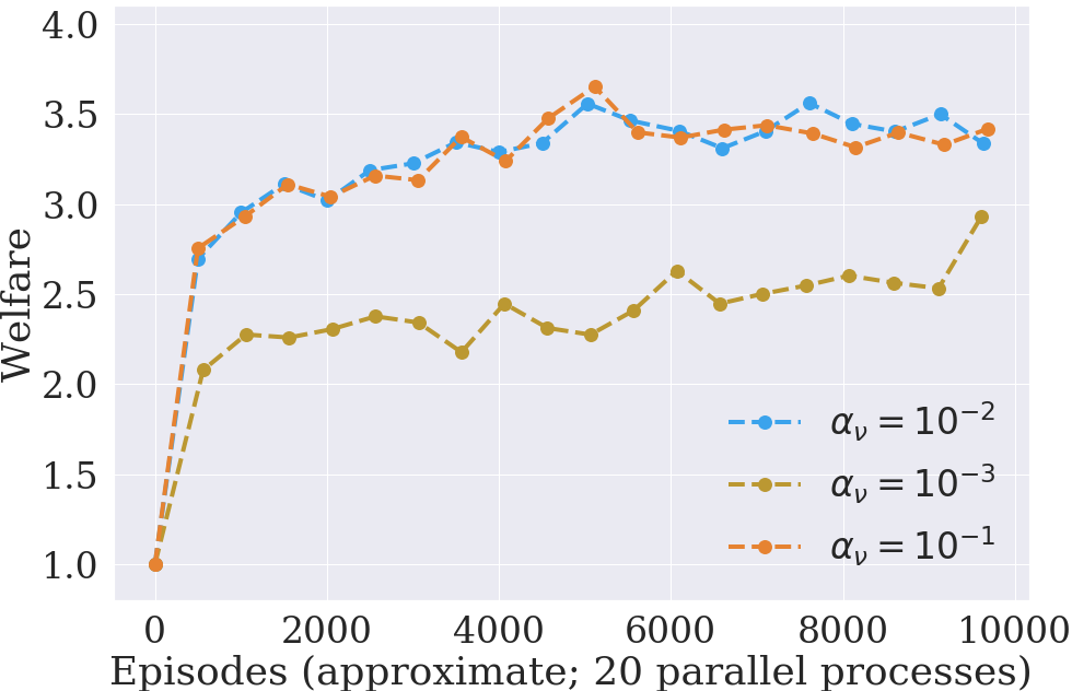
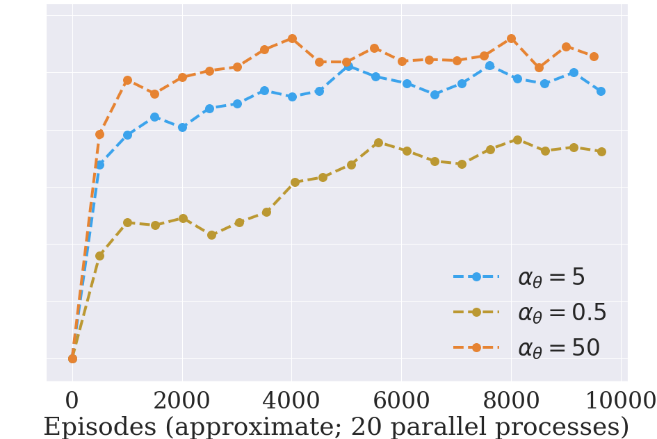
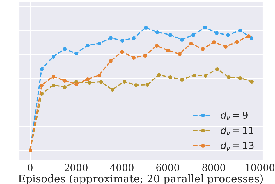
Note: Training was performed in 20 parallel processes. Each point is an average over 500 evaluation episodes. A welfare of $1$ corresponds to a random policy (50% treatment probability). The main specification uses $\alpha_{\theta}=5,\alpha_{\nu}=10^{-2},d_{\nu}=9$.

Figure 6.3. Sensitivity to tuning parameters

6.2.2. Results

Figure 6.4 shows the result from running our baseline implementation for our policy classes. We also compare our policies, which are both solutions to a dynamic programming problem, to that obtained from the EWM method of Kitagawa and Tetenov (2018) under a budget constraint of $0.25$. We use the same rewards and apply their methods on the policy class $\mathbb{I}(\theta_{0}+\theta_{1}^{\intercal}{\bf x})$ - which is just a deterministic version of our soft-max class. As noted earlier, the objective function in EWM maximizes in-sample welfare, and is meant to be simultaneously applied on the population. The use of discounting, and the fact that the distribution of arrivals varies within the year require the optimal policy to be derived using dynamic programming methods. These are important aspects of the optimization problem. Dropping them has severe consequences: we see a 25% higher welfare on average under both our proposed policies. At the same time, there is not much gain from employing non-stationary policies in this example, the increase in welfare being less than $1\%$. In this specific example, the stationary policy turns out to be very attractive for a policy maker.

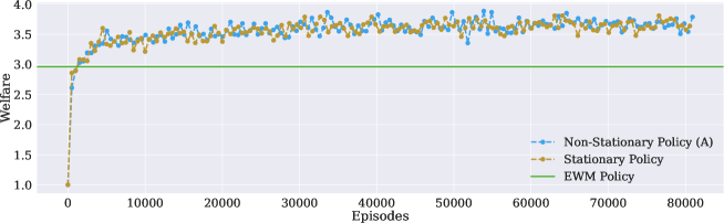
Note: The stationary policy does not include budget or time but is computed by the RL algorithm as a solution to a dynamic programming problem (with a value function that still contains budget and time). The EWM policy assumes the problem to be static. Training was performed in 20 parallel processes. Each point is an average over 500 evaluation episodes. A welfare of $1$ corresponds to a random policy (50% treatment probability).

Figure 6.4. Convergence of episodic welfare

Figure 6.5 displays the convergence of the policy coefficients for the non-stationary policy class A. The relative values of the coefficients (in the figure this is relative to the intercept) converge rather fast. The coefficients, however, keep increasing slowly in absolute value, which makes the policy more deterministic (i.e. the action probabilities closer to either 0 or 1). In practice, we can thus truncate the training episodes early and convert the soft-max policy rule to a deterministic one (i.e., treat if treatment probability is larger than 50%). With this deterministic version of our policy, we achieve 28% higher welfare compared to EWM.

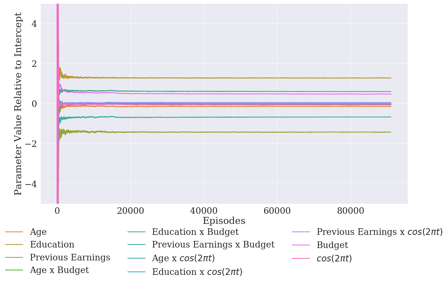
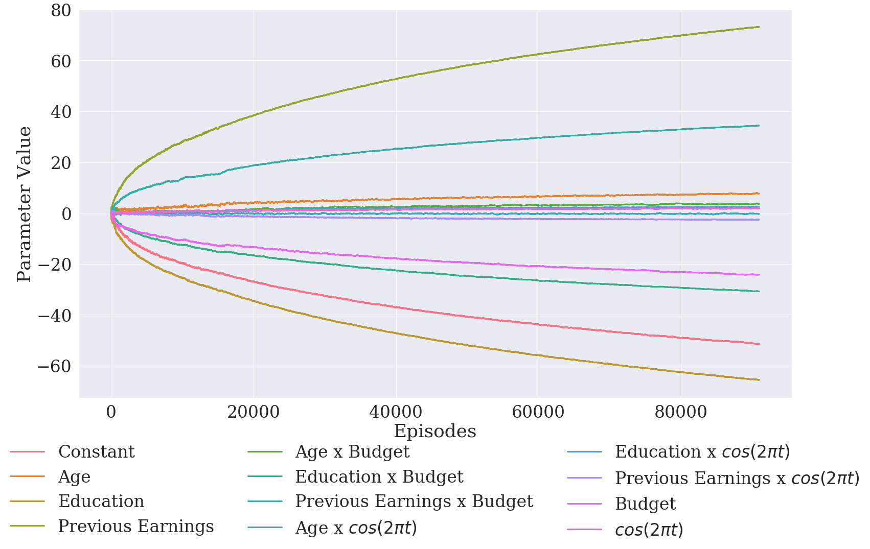
A: Relative Coefficients over the Course of Training

B: Coefficients over the Course of Training

Figure 6.5. Convergence of policy function coefficients

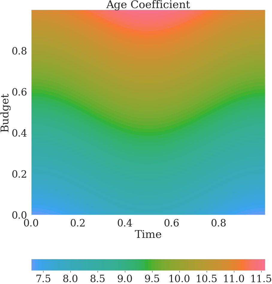
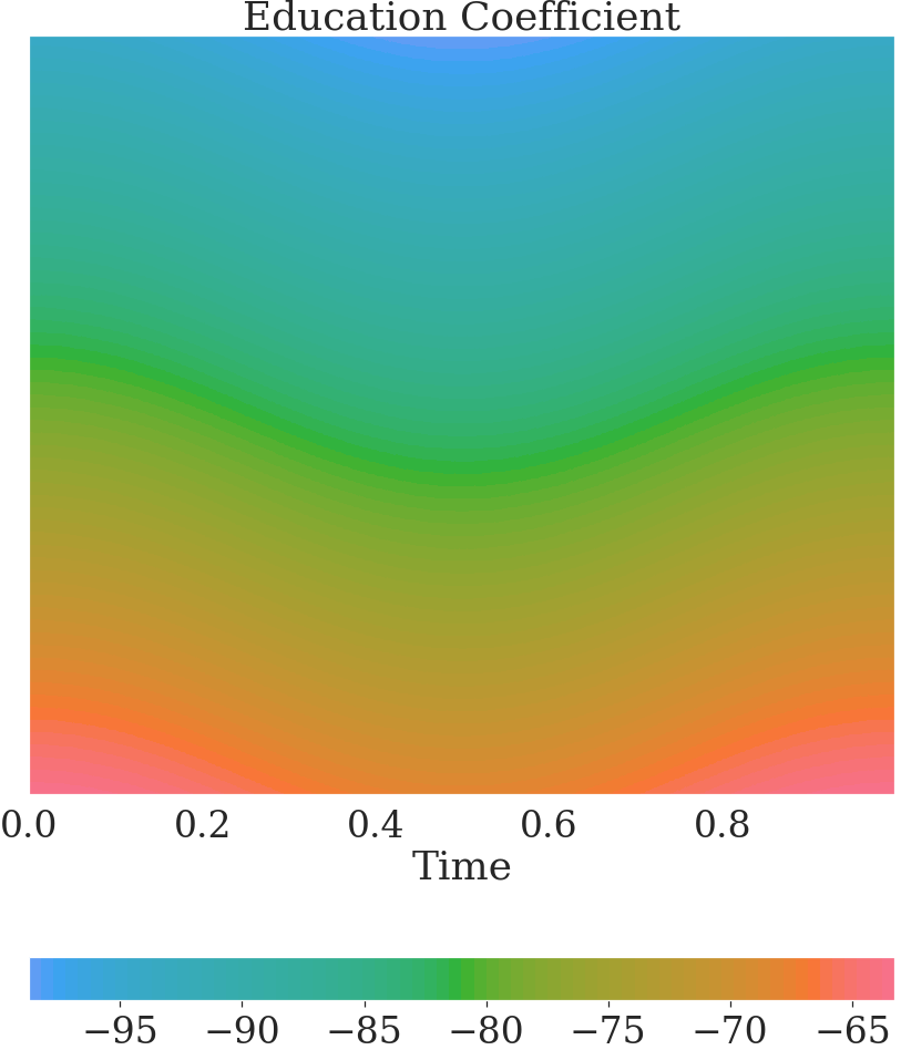
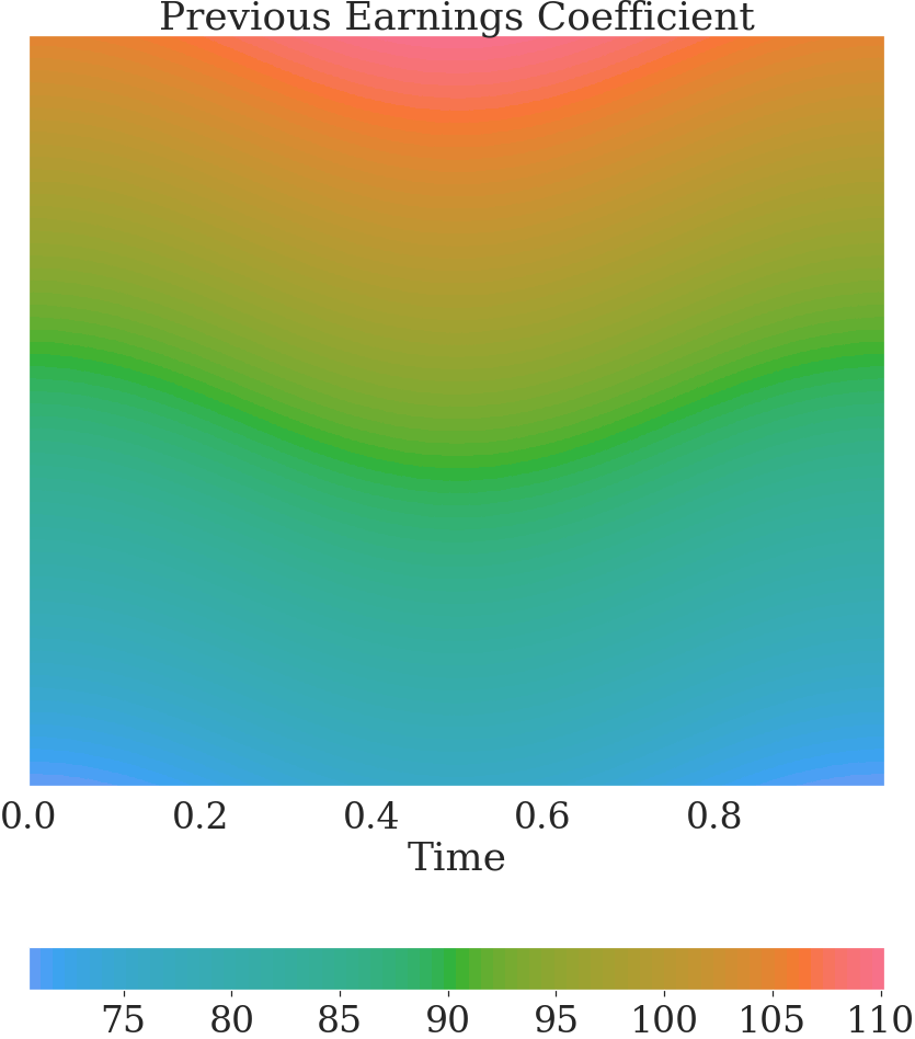
Figure 6.6. Coefficient interactions in the non-stationary policy (A)

In the non-stationary policy class A, time and budget influence how the covariates affect the treatment decision. Figure 6.6 indicates how large the coefficient value corresponding to each covariate is, after including interactions with time and budget. Specifically, if we write $\pi_{\theta}$ in the form $\log(\pi_{\theta}/(1-\pi_{\theta})=\theta_{0}+\theta_{a1}\textrm{age}+\theta_{a2}z\cdot\textrm{age}+\theta_{a3}\cos(2\pi t)\cdot\textrm{age}+...$, then age affects the treatment decision with the coefficient $\theta_{a}(z,t)=\theta_{a1}+\theta_{a2}z+\theta_{a3}\cos(2\pi t)$, which we plot. Based on the heatmaps we find, e.g., that older individuals are more likely to be treated at the beginning of the year. Similar comments apply to policy class B (results not shown).

In summary, the example shows that RL algorithms can increase welfare in the challenging dynamic decision settings faced by economic policy makers. While the use of the JTPA data allows us to compare our approach to recent work, the dynamic environment we use to illustrate the potential of RL solutions is already of considerable complexity. Indeed, our policy function (with interactions) contains 12 coefficients.

7. Conclusion

In this paper, we have shown how RL can be combined with data from RCTs to obtain dynamic assignment rules under constraints. Our framework is general and incorporates a range of settings of practical importance (for an extension to non-compliance, see the supplementary material). Furthermore, it can utilize large amounts of existing RCT data. As A3C algorithms scale to problems with much higher dimensional state spaces (see e.g. Mnih et al, 2016), the approach is very flexible and applicable to an array of datasets and real world decision problems which policy makers face. The ability of RL methods to take into account large amounts of state variables when personalizing treatments could also give incentives to run targeted studies with many recorded covariates.

At the same time, the work raises a number of avenues for future research. One interesting avenue would be to study how existing RCT data can be used not only to train a policy function as in our examples, but also to employ further online learning to fine-tune the initialized policy to current data. We have also assumed that individuals do not respond strategically to non-stationary policies. However, if they do and the response is known or estimable, this could be directly included in our setup. Furthermore, our methodology requires the social-planner to pre-select a class of policy rules, but it is silent on how this class is to be chosen. In reality, the planner must balance various welfare and ethical tradeoffs in choosing the policy class, e.g., in choosing which covariates to include. The planner may note that more covariates may lead to higher welfare, but also more possibilities for statistical discrimination. In future work, it would be particularly interesting to study how “ethical constraints” can be added to the RL environment and reward structure, such as changing the welfare criterion so that rewards are higher if certain target allocations are met. This would help develop algorithms that aid economic policy making while directly taking wider ethical considerations into account.

For Online Publication

Appendix to:

DYNAMICALLY OPTIMAL TREATMENT ALLOCATION USING REINFORCEMENT LEARNING

Karun Adusumilli^⋆, Friedrich Geiecke^† & Claudio Schilter^‡

^⋆Department of Economics, University of Pennsylvania; akarun@sas.upenn.edu
^†Department of Methodology, London School of Economics; f.c.geiecke@lse.ac.uk
^‡Department of Economics, University of Zurich; claudio.schilter@econ.uzh.ch

Supplementary material for this paper (not intended for publication) can be accessed here.

Appendix A Proofs of main results

We start by recalling the definition of a viscosity solution. We focus here on the Dirichlet boundary condition. The other boundary conditions are discussed in Appendix B.

Consider the Dirichlet problem

(A.1) $$F\left(z,t,u(z,t),Du(z,t)\right)=0\textrm{ on }\text{$\mathcal{U}$};\quad u=0\textrm{ on }\text{$\Gamma$},$$

where $Du$ denotes the derivative with respect to $(z,t)$, $\mathcal{U}$ is the domain of the PDE, and $\Gamma\subseteq\partial\mathcal{U}$ is the set on which the boundary condition is specified. In what follows, let $y:=(z,t)$. Also, $\mathcal{C}^{2}(\mathcal{U})$ denotes the space of all twice continuously differentiable functions on $\mathcal{U}$.

Definition 1.

A bounded continuous $u(\cdot)$ is a viscosity sub-solution to (A.1) if:

(i) $u\leq 0$ on $\Gamma$, and

(ii) for each $\phi\in\mathcal{C}^{2}(\mathcal{U})$, if $u-\phi$ has a local maximum at $y\in\mathcal{U}$, then

$$F\left(y,u(y),D\phi(y)\right)\leq 0.$$

Similarly, a bounded continuous $u(\cdot)$ is a viscosity super-solution to (A.1) if:

(i) $u\geq 0$ on $\Gamma$, and

(ii) for each $\phi\in\mathcal{C}^{2}(\mathcal{U})$, if $u-\phi$ has a local minimum at $y\in\mathcal{U}$, then

$$F\left(y,u(y),D\phi(y)\right)\geq 0.$$

Finally, $u$ is a viscosity solution to (A.1) if it is both a sub- and a super-solution.

We say that $u$ is a viscosity sub-solution to (A.1) on $\mathcal{U}$ if only condition (ii) holds, i.e., it need not be the case that $u\leq 0$ on $\Gamma$. Similarly, $u$ is a viscosity super-solution to (A.1) on $\mathcal{U}$ if only condition (ii) holds. Henceforth, whenever we refer to a viscosity super- or sub-solution, we will implicitly assume that it is bounded and continuous.

We say that a PDE is in Hamiltonian form if

$$F\left(y,u(y),Du(y)\right)=\partial_{t}u(y)+H(y,u(y),\partial_{z}u(y)),$$

for some Hamiltonian $H(\cdot)$. Suppose that the PDE (A.1) can be written in Hamiltonian form. Then there exists a unique viscosity solutions to (A.1) if the following regularity conditions are satisfied (see, e.g., Crandall et al, 1992):

• $H(y,u,p)$ is uniformly continuous in all its arguments.

• There exists a modulus of continuity $\omega(\cdot)$ such that $\forall\ (y_{1},y_{2})\in\mathcal{U}$,

  $$\left|H(y_{1},u,p_{1})-H(y_{2},u,p_{2})\right| \leq\omega\left(\left\|y_{1}-y_{2}\right\|+\left\|p_{1}-p_{2}\right\|\right),\quad\textrm{and}$$

  $$\left|H(y_{1},u,p_{1})-H(y_{2},u,p_{1})\right| \leq\omega\left(\left\|y_{1}-y_{2}\right\|\left|1+\left\|p_{1}\right\|\right|\right).$$

• $H(y,u,p)\ \textrm{is non-decreasing in $u$ for all $(y,p)$.}$

• There exist some viscosity sub- and super-solutions to PDE (A.1).

A.1. Proof of Lemma 1

We prove the lemma for the Dirichlet boundary condition. The other boundary conditions are discussed in Appendix B. Consider the PDE

(A.2) $$\partial_{\tau}u_{\theta}+H_{\theta}(z,\tau,\partial_{z}u_{\theta}) =0\quad\textrm{on }\Upsilon\equiv(\underline{z},\infty)\times(0,T];$$

$$u_{\theta} =0\quad\textrm{on }\mathcal{B}\equiv\{\{\underline{z}\}\times[0,T]\}\cup\{(\underline{z},\infty)\times\{0\}\},$$

where $H_{\theta}(\cdot)$ is defined as

(A.3) $$H_{\theta}(z,\tau,p):=-e^{\beta\tau}\lambda(\tau)\bar{r}_{\theta}(z,\tau)-\lambda(\tau)\bar{G}_{\theta}(z,\tau)p.$$

Let $u_{\theta}$ denote a viscosity solution to (A.2). By Lemma G.1 in Appendix G and the subsequent discussion, there is a one-to-one transformation between $u_{\theta}$ and any solution, $h_{\theta}$, for PDE (2.3) under the Dirichlet boundary condition (2.7); this transformation is given by $h_{\theta}(z,t):=e^{-\beta(T-t)}h_{\theta}(z,T-t)$. Hence, $h_{\theta}$ exists and is unique if and only if $u_{\theta}$ also exists and is unique.

It thus suffices to show existence of a unique solution for (A.2). It is straightforward to verify that the function $H_{\theta}(\cdot)$ satisfies the regularity conditions (R1)-(R3) under Assumption 1. Furthermore, the set $\mathcal{B}$ satisfies the uniform exterior sphere condition. When these properties are satisfied, Crandall (1997, Section 9) shows that a unique viscosity solution exists for (A.2), as long as (R4) is satisfied, i.e., we are able to exhibit continuous sub- and super-solutions to (A.2). Under Assumption 1, it can be verified that one such set is $-L\tau$ and $L\tau$, where $L<\infty$ is chosen to satisfy $|\lambda(\tau)\bar{r}_{\theta}(z,\tau)|\leq M\sup_{\tau}\lambda(\tau)<L$.

A.2. Proof of Theorem 1

The following proof is based on an argument first sketched by Souganidis (2009). We focus here on the Dirichlet boundary condition with $T<\infty$ (but $\underline{z}$ could be $-\infty$). The argument for the setting with $T=\infty$ is similar, so we omit it. We also omit the proof for the periodic boundary condition since it follows by the same reasoning (and is in fact simpler since we do not need to consider separate cases for regions close to the boundary).

All the statements in this section should be understood to be holding with probability approaching $1$. In what follows, we drop this qualification for ease of notation and hold this to be implicit. We also employ the following notation: For any function $f$ over $(z,t)$, $Df$ denotes its Jacobean. Additionally, $\left\|\partial_{z}f\right\|,\left\|\partial_{z}f\right\|$ and $\left\|Df\right\|$ denote the Lipschitz constants for $f(\cdot,t),f(z,\cdot)$ and $f(\cdot,\cdot)$.

We represent PDE (3.2) by

(A.4) $$F_{\theta}(z,t,f,\partial_{z}f,\partial_{t}f) =0\ \textrm{on $\mathcal{U}$};\quad f=0\ \textrm{on $\Gamma$},$$

with $f$ denoting a function, and where

$$F_{\theta}(z,t,l,p,q) :=-\lambda(t)\bar{G}_{\theta}(z,t)l-p+\beta q-\lambda(t)\bar{r}_{\theta}(z,t).$$

Additionally, denote our approximation scheme (3.5) by

(A.5) $$S_{\theta}([f],f(z,t),z,t) =0\ \textrm{on $\mathcal{U}$};\quad f=0\ \textrm{on $\Gamma$},$$

where for any two functions $f_{1},f_{2}$,

(A.6) $$S_{\theta}\left([f_{1}],f_{2}(z,t),z,t,b_{n}\right):=b_{n}\lambda(t)\left(f_{2}(z,t)-E_{n,\theta}\left[e^{-\beta(t^{\prime}-t)}f_{1}(z^{\prime},t^{\prime})|z,t\right]\right)-\lambda(t)\hat{r}_{\theta}(z,t).$$

Here $[f]$ refers to the fact that it is a functional argument. Note that $h_{\theta}$ and $\tilde{h}_{\theta}$ are the functional solutions to (A.4) and (A.5) respectively. We make use of the following two properties of $S_{\theta}(\cdot)$: First, $S_{\theta}(\cdot)$ is monotone in its first argument, i.e.,

(A.7) $$S_{\theta}([f_{1}],f(z,t),z,t,b_{n})\geq S_{\theta}([f_{2}],f(z,t),z,t,b_{n})\ \forall\ f_{2}\geq f_{1}.$$

Second, for any $r\in\mathbb{R}$ and $m\in\mathbb{R}^{+}$, it holds for all $t\leq T-b_{n}^{-1/2}$ that

(A.8) $$S_{\theta}([f+m],r+m,z,t,b_{n})\geq S_{\theta}([f],r,z,t)+\chi m,$$

where $\chi=\beta+O(b_{n}^{-1})>0$. The first property is trivial to show. As for the second, under Assumption 1 and $t\leq T-b_{n}^{-1/2}$, it is straightforward to show

$$S_{\theta}([f+m],r+m,z,t,b_{n})-S_{\theta}([f],r,z,t) =mb_{n}\lambda(t)\left(1-E_{n,\theta}\left[e^{-\beta(t^{\prime}-t)}|z,t\right]\right)$$

$$=m(\beta+O(b_{n}^{-1})).$$

Our proof also makes use of Lemmas G.2 and G.3, which ensure there exists $K_{1}<\infty$ such that

(A.9) $$\left\|h_{\theta}\right\|<K_{1},\quad\textrm{and }\ \sup_{\theta}\left\|Dh_{\theta}\right\| <K_{1}.$$

We provide here an upper bound for

(A.10) $$m_{\theta}:=\sup_{(z,t)\in\bar{\mathcal{U}}}\left(h_{\theta}(z,t)-\tilde{h}_{\theta}(z,t)\right).$$

A lower bound for $h_{\theta}-\tilde{h}_{\theta}$ can be obtained analogously. Clearly, we may assume $m_{\theta}>0$, as otherwise we are done. Denote $(z_{\theta}^{*},t_{\theta}^{*})$ as the point at which the supremum is attained in (A.10) (or, if such a point does not exist, where the right hand side of (A.10) is arbitrarily close to $m_{\theta}$). We consider three (not necessarily mutually exclusive) cases: (i) $|t_{\theta}^{*}-T|\leq 2K_{1}\epsilon$, (ii) $|z_{\theta}^{*}-\underline{z}|\leq 2K_{1}\epsilon$, and (iii) $|z_{\theta}^{*}-\underline{z}|>2K_{1}\epsilon$ and $|t_{\theta}^{*}-T|>2K_{1}\epsilon$. Here, $\epsilon$ is any positive number satisfying $\epsilon\geq\sqrt{b_{n}}$.

We start with Case (i). In view of (A.9), and the fact $|t_{\theta}^{*}-T|\leq 2K_{1}\epsilon$, we have

(A.11) $$|h_{\theta}(z_{\theta}^{*},t_{\theta}^{*})|\leq 4K_{1}^{2}\epsilon.$$

Now, we claim $\tilde{h}_{\theta}(z,t)\leq L\{(T-t)+b_{n}^{-1}\}$, for some $L<\infty$ independent of $\theta,z,t$. Let $N[t,T]$ be a random variable denoting the number of arrivals between $t$ and the end point $T$. Then $N[t,T]$ is first order stochastically dominated by $\bar{N}[t,T]\sim\textrm{Poisson}(\bar{\lambda}b_{n}(T-t))$, where $\bar{\lambda}:=\sup_{t}\lambda(t)<\infty$. Hence, $E[N[t,T]]\leq E[\bar{N}[t,T]]=\bar{\lambda}b_{n}(T-t)$. Furthermore, the reward from any given arrival is at most $\sup_{\theta,z,t}|\hat{r}_{\theta}(z,t)|/b_{n}\leq 2M/b_{n}$ by Assumption 2(i) and (A.31). Consequently,

$$\tilde{h}_{\theta}(z,t)\leq\frac{2M}{b_{n}}+E\left[N[t,T]\frac{2M}{b_{n}}\right]\leq 2M\bar{\lambda}\left\{(T-t)+b_{n}^{-1}\right\}:=L\left\{(T-t)+b_{n}^{-1}\right\}.$$

Considering that we are in the case $|t_{\theta}^{*}-T|\leq 2K_{1}\epsilon$, the previous statement implies

(A.12) $$|\tilde{h}_{\theta}(z_{\theta}^{*},t_{\theta}^{*})|\leq L\left(2K_{1}\epsilon+b_{n}^{-1}\right).$$

In view of (A.11) and (A.12), we thus obtain

(A.13) $$m_{\theta}\leq(4K_{1}^{2}+2LK_{1})\epsilon+Lb_{n}^{-1}.$$

This completes the treatment of the first case, when $|t_{\theta}^{*}-T|\leq 2K_{1}\epsilon$.

We next consider Case (ii). At the end of this proof, we show that when $\bar{G}_{\theta}(z,t)<-\delta$ (cf. Assumption 2(ii)), the expected number of arrivals subsequent to state $z$ is bounded above by $2\delta^{-1}\left\{b_{n}(z-\underline{z})+C_{1}\right\}$ for some $C_{1}<\infty$ independent of $\theta,z,t$. Hence, by a similar argument as that leading to (A.12), we have $|\tilde{h}_{\theta}(z_{\theta}^{*},t_{\theta}^{*})|\leq L_{2}\{2K_{1}\epsilon+b_{n}^{-1}\}$ for some $L_{2}<\infty$. Combined with the Lipschitz continuity of $h_{\theta}$, this implies the bound (A.13) also holds for Case (ii).

We now turn to Case (iii), i.e., $|z_{\theta}^{*}-\underline{z}|>2K_{1}\epsilon$ and $|t_{\theta}^{*}-T|>2K_{1}\epsilon$. Denote

$$\mathcal{A}\equiv\{(z,t)\in\bar{\mathcal{U}}:\ |z-\underline{z}|>2K_{1}\epsilon\ \cap\ |t-T|>2K_{1}\epsilon\}.$$

Let $h_{\theta}^{\epsilon}(z,t)$ denote the sup-convolution of $h_{\theta}(z,t)$:

$$h_{\theta}^{\epsilon}(z,t):=\sup_{(r,w)\in\bar{\mathcal{U}}}\left\{h_{\theta}(r,w)-\frac{1}{\epsilon}\left(|r-z|^{2}+|w-t|^{2}\right)\right\}.$$

We make use of the following properties of $h_{\theta}^{\epsilon}:$ First, $h_{\theta}^{\epsilon}$ is a semi-convex function with coefficient $1/\epsilon$ (Lemma H.2). Second, by (A.9) and Lemma H.2,

(A.14) $$\sup_{(z,t)\in\bar{\mathcal{U}}}\left|h_{\theta}(z,t)-h_{\theta}^{\epsilon}(z,t)\right|\leq 4K_{1}^{2}\epsilon,\ \textrm{and }$$

(A.15) $$\sup_{\theta}\left\|Dh_{\theta}^{\epsilon}\right\|\leq 4\sup_{\theta}\left\|Dh_{\theta}\right\|\leq 4K_{1}.$$

Third, by Lemma H.3 (Assumption 1 ensures all relevant regularity conditions for $F_{\theta}(\cdot)$ are satisfied), there exists $c<\infty$ independent of $(\theta,z,t)$ such that, in a viscosity sense,

(A.16) $$F_{\theta}(z,t,h_{\theta}^{\epsilon},\partial_{z}h_{\theta}^{\epsilon},\partial_{t}h_{\theta}^{\epsilon})\leq c\epsilon\quad\textrm{on }\mathcal{A}.$$

We now compare $S_{\theta}(\cdot)$ and $F_{\theta}(\cdot)$ at the function $h_{\theta}^{\epsilon}$. Consider any $(z,t)\in\mathcal{A}$. If $h_{\theta}^{\epsilon}$ is not differentiable at $(z,t)$, let $(\dot{z},\dot{t})$ denote a point arbitrarily close to $(z,t)$ where it is indeed differentiable (note that $h_{\theta}^{\epsilon}$ is Lipschitz continuous, so this point can be chosen as close to $(z,t)$ as one wants). We can then expand

$$S_{\theta}([h_{\theta}^{\epsilon}],h_{\theta}^{\epsilon}(z,t),z,t,b_{n}) \cong S_{\theta}([h_{\theta}^{\epsilon}],h_{\theta}^{\epsilon}(\dot{z},\dot{t}),z,t,b_{n})$$

(A.17) $$=b_{n}\lambda(t)h_{\theta}^{\epsilon}(\dot{z},\dot{t})\left(1-E_{n,\theta}\left[e^{-\beta(t^{\prime}-t)}|z,t\right]\right)$$

$$\ +b_{n}\lambda(t)E_{n,\theta}\left[e^{-\beta(t^{\prime}-t)}\left\{h_{\theta}^{\epsilon}(\dot{z},\dot{t})-h_{\theta}^{\epsilon}(z^{\prime},t^{\prime})\right\}|z,t\right]+(-1)\lambda(t)\hat{r}_{\theta}(z,t)$$

(A.18) $$:=A_{\theta}^{(1)}(z,t)+A_{\theta}^{(2)}(z,t)+A_{\theta}^{(3)}(z,t),$$

where the notation ‘$\cong$’ in the first step indicates that we are performing the arbitrarily small approximation of replacing $h_{\theta}^{\epsilon}(z,t)$ in the second argument of $S_{\theta}(\cdot)$ with $h_{\theta}^{\epsilon}(\dot{z},\dot{t})$ - recall that $S_{\theta}(\cdot)$ is linear in its second argument and $h_{\theta}^{\epsilon}$ is Lipschitz continuous. Using $\left\|h_{\theta}^{\epsilon}\right\|\leq\left\|h_{\theta}\right\|\leq K_{1}$ and Assumptions 1-4, it is straightforward to show

(A.19) $$A_{\theta}^{(1)}(z,t)\leq\beta h_{\theta}^{\epsilon}(\dot{z},\dot{t})+\frac{C_{1}}{b_{n}},$$

for some $C_{1}$ independent of $\theta,z,t$. Next, consider $A_{\theta}^{(2)}(z,t)$. By semi-convexity of $h_{\theta}^{\epsilon}$ (see, Lemma H.1),

$$h_{\theta}^{\epsilon}(z^{\prime},t^{\prime}) \geq h_{\theta}^{\epsilon}(\dot{z},\dot{t})+\partial_{z}h_{\theta}^{\epsilon}(\dot{z},\dot{t})(z^{\prime}-\dot{z})+\partial_{t}h_{\theta}^{\epsilon}(\dot{z},\dot{t})(t^{\prime}-\dot{t})-\frac{1}{2\epsilon}\left\{|z^{\prime}-\dot{z}|^{2}+|t^{\prime}-\dot{t}|^{2}\right\}$$

$$\cong h_{\theta}^{\epsilon}(\dot{z},\dot{t})+\partial_{z}h_{\theta}^{\epsilon}(\dot{z},\dot{t})(z^{\prime}-z)+\partial_{t}h_{\theta}^{\epsilon}(\dot{z},\dot{t})(t^{\prime}-t)-\frac{1}{2\epsilon}\left\{|z^{\prime}-z|^{2}+|t^{\prime}-t|^{2}\right\},$$

where we again employ the arbitrarily small approximation of replacing $\dot{z},\dot{t}$ in the second step with $z,t$ (note that (A.15) ensures $\partial_{z}h_{\theta}^{\epsilon},\partial_{t}h_{\theta}^{\epsilon}$ are uniformly bounded). Substituting the above into the expression for $A_{\theta}^{(2)}(z,t)$, and using Assumption 1, (A.31) and (A.15), some straightforward algebra enables us to show that when $\epsilon\geq b_{n}^{-1/2}$,

$$A_{\theta}^{(2)}(z,t) \leq-\lambda(t)\bar{G}_{\theta}(z,t)\partial_{z}h_{\theta}^{\epsilon}(\dot{z},\dot{t})-\partial_{t}h_{\theta}^{\epsilon}(\dot{z},\dot{t})+C_{2}\left(\frac{1}{\epsilon b_{n}}+\sqrt{\frac{v}{n}}\right)$$

(A.20) $$\cong-\lambda(\dot{t})\bar{G}_{\theta}(\dot{z},\dot{t})\partial_{z}h_{\theta}^{\epsilon}(\dot{z},\dot{t})-\partial_{t}h_{\theta}^{\epsilon}(\dot{z},\dot{t})+C_{2}\left(\frac{1}{\epsilon b_{n}}+\sqrt{\frac{v}{n}}\right),$$

where $C_{2}$ is again independent of $(\theta,z,t)$, and we have made use of the continuity of $\lambda(\cdot),\bar{G}_{\theta}(\cdot)$ in the second step. Finally, to bound $A_{\theta}^{(3)}(z,t)$, we make use of Assumption 1(ii) and (A.31), which together ensure there exists $C_{3}$ independent of $\theta,z,t$ such that

$$A_{\theta}^{(3)}(z,t) \leq-\lambda(t)\bar{r}_{\theta}(z,t)+C_{3}\sqrt{\frac{v}{n}}$$

(A.21) $$\cong-\lambda(\dot{t})\bar{r}_{\theta}(\dot{z},\dot{t})+C_{3}\sqrt{\frac{v}{n}}.$$

Combining (A.18)-(A.21), and setting $C=\max(C_{1},C_{2},C_{3})$, we thus find

(A.22) $$S_{\theta}([h_{\theta}^{\epsilon}],h_{\theta}^{\epsilon}(z,t),z,t,b_{n})\leq F_{\theta}(\dot{z},\dot{t},h_{\theta}^{\epsilon},\partial_{z}h_{\theta}^{\epsilon},\partial_{t}h_{\theta}^{\epsilon})+C\left\{\frac{1}{b_{n}}\left(1+\frac{1}{\epsilon}\right)+\sqrt{\frac{v}{n}}\right\}.$$

In view of (A.22) and (A.16),

(A.23) $$S_{\theta}([h_{\theta}^{\epsilon}],h_{\theta}^{\epsilon}(z,t),z,t,b_{n})\leq c\epsilon+C\left\{\frac{1}{b_{n}}\left(1+\frac{1}{\epsilon}\right)+\sqrt{\frac{v}{n}}\right\}.$$

Let (here $f^{+}:=\max(f,0))$

$$m_{\theta}^{\epsilon}:=\sup_{(z,t)\in\mathcal{A}}\left(h_{\theta}^{\epsilon}(z,t)-\tilde{h}_{\theta}(z,t)\right)^{+},$$

and denote $(\breve{z}_{\theta},\breve{t}_{\theta})$ as the point at which the supremum is attained (or where the right hand side of the above expression is arbitrarily close to $m_{\theta}^{\epsilon}$). Now, by definition,

$$h_{\theta}^{\epsilon}\leq\tilde{h}_{\theta}+m_{\theta}^{\epsilon}\ \textrm{on }\mathcal{A}.$$

Then, in view of the properties (A.7), (A.8) of $S(\cdot)$,

$$\chi m_{\theta}^{\epsilon} =S_{\theta}\left([\tilde{h}_{\theta}],\tilde{h}_{\theta}(\breve{z}_{\theta},\breve{t}_{\theta}),\breve{z}_{\theta},\breve{t}_{\theta},b_{n}\right)+\chi m_{\theta}^{\epsilon}$$

(A.24) $$\leq S_{\theta}\left([\tilde{h}_{\theta}+m_{\theta}^{\epsilon}],\tilde{h}_{\theta}(\breve{z}_{\theta},\breve{t}_{\theta})+m_{\theta}^{\epsilon},\breve{z}_{\theta},\breve{t}_{\theta},b_{n}\right)$$

$$\leq S_{\theta}\left([h_{\theta}^{\epsilon}],h_{\theta}^{\epsilon}(\breve{z}_{\theta},\breve{t}_{\theta}),\breve{z}_{\theta},\breve{t}_{\theta},b_{n}\right).$$

Combining (A.24) and (A.23) gives

(A.25) $$m_{\theta}^{\epsilon}\leq c_{1}\epsilon+C\left\{\frac{1}{b_{n}}\left(1+\frac{1}{\epsilon}\right)+\sqrt{\frac{v}{n}}\right\},$$

where $c_{1}=\chi^{-1}c$ and $C_{1}=\chi^{-1}C$ are independent of $\theta,z,t$. Hence, in view of (A.14) and (A.25),

(A.26) $$m_{\theta}\leq(4K_{1}^{2}+c_{1})\epsilon+C_{1}\left\{\frac{1}{b_{n}}\left(1+\frac{1}{\epsilon}\right)+\sqrt{\frac{v}{n}}\right\}.$$

This completes the derivation of the upper bound for $m_{\theta}$ under Case (iii).

Finally, in view of (A.13) and (A.26), setting $\epsilon=b_{n}^{-1/2}$ gives the desired rate.

Bound on expected number of arrivals after $z$

It remains to show that the expected number of arrivals subsequent to a state with institutional variable $z$ is bounded by $2\delta^{-1}\left\{b_{n}(z-\underline{z})+C_{1}\right\}$, as was needed for the analysis of Case (ii). Denote by $\{\bar{s}_{i}\equiv(x_{i},z_{i},t_{i},a_{i}):i=1,2,\dots\}$ the sequence of state-action variables following any particular state-action variable $\bar{s}_{0}=(x,z,t,a)$, and let

$$M_{l}:=\sum_{i=1}^{l}\left\{G_{a_{i}}(x_{i},z_{i},t_{i})-\hat{G}_{\theta}(z_{i},t_{i})\right\}.$$

Clearly, $M_{l}$ is a martingale with respect to the filtration $\mathcal{F}_{l}:=\sigma(\bar{s}_{l-1},\dots,\bar{s}_{0})$. Let $\mathcal{N}[\bar{s}_{0}]$ be the random variable denoting the number of arrivals following $\bar{s}_{0}$, until either $z$ goes below $\underline{z}$ or time runs out. Then $\mathcal{N}[\bar{s}_{0}]=\tau[\bar{s}_{0}]-1$, where $\tau[\bar{s}_{0}]$ is the stopping time

$$\tau[\bar{s}_{0}]:=\inf\left\{l\in\{1,2,\dots\}:G_{a}(x,z,t)+\sum_{i=1}^{l-1}G_{a_{i}}(x_{i},z_{i},t_{i})\leq-b_{n}(z-\underline{z})\ \textrm{or}\ t_{l-1}\geq T\right\}.$$

Now, Assumption 2(i) implies the martingale differences of $M_{l}$ are bounded. Hence, we can apply the Optional Stopping Theorem to obtain

$$E_{n,\theta}\left[M_{\tau[\bar{s}_{0}]}\right]=E_{n,\theta}[M_{1}]=0.$$

In other words,

$$E_{n,\theta}\left[\sum_{i=1}^{\tau[\bar{s}_{0}]}G_{a_{i}}(x_{i},z_{i},t_{i})-\sum_{i=1}^{\tau[\bar{s}_{0}]}\hat{G}_{\theta}(z_{i},t_{i})\right]=0.$$

By Assumption 2(ii) and (A.31), $-\sum_{i=1}^{\tau[\bar{s}_{0}]}\hat{G}_{\theta}(z_{i},t_{i})\geq(\delta/2)\tau[\bar{s}_{0}]$. Furthermore, by the definition of $\tau[\bar{s}_{0}]$ and the assumption $\left|G_{a}(s)\right|\leq M$, we have

$$E_{n,\theta}\left[\sum_{i=1}^{\tau[\bar{s}_{0}]}G_{a_{i}}(x_{i},z_{i},t_{i})\right] \geq E_{n,\theta}\left[\mathbb{I}(\tau[\bar{s}_{0}]\geq 2)\left\{G_{a}(x,z,t)+\sum_{i=1}^{\tau[\bar{s}_{0}]-2}G_{a_{i}}(x_{i},z_{i},t_{i})\right\}\right]-3M$$

$$>-b_{n}(z-\underline{z})-3M.$$

The above implies $(\delta/2)E_{n,\theta}[\tau[\bar{s}_{0}]]<b_{n}(z-\underline{z})+3M$ or $E_{n,\theta}[\mathcal{N}[\bar{s}_{0}]]<2\delta^{-1}\{b_{n}(z-\underline{z})+C_{1}\}$ where $C_{1}:=3M$. Note that this bound is independent of $(x,t,a)$ in the definition of $\bar{s}_{0}$.

A.3. Proof of Theorem 2

Here, we prove the result for the Dirichlet boundary condition. The proofs for the other boundary conditions are in Appendix B. Within the Dirichlet boundary condition, there are two further sub-cases, depending on whether $T<\infty$ or $T=\infty$. For our proof we choose the case of $T<\infty$. We will later sketch how the proof can be modified to deal with the other, arguably simpler, case where $T=\infty$ (but $\underline{z}>-\infty$).

Without loss of generality, we may set $t_{0}=0$. As in the proof of Lemma 1, we make a change of variable $\tau(t):=T-t$, and employ the transformation $u_{\theta}(z,\tau):=e^{\beta\tau}h_{\theta}(z,T-\tau)$. Note that $u_{\theta}$ is the viscosity solution to (A.2). Similarly, we also define $\hat{u}_{\theta}(z,\tau):=e^{\beta\tau}\hat{h}_{\theta}(z,T-\tau)$, and note that $\hat{u}_{\theta}$ is the viscosity solution to

(A.27) $$\partial_{\tau}\hat{u}_{\theta}+\hat{H}_{\theta}(z,\tau,\partial_{z}\hat{u}_{\theta}) =0\ \textrm{on }\Upsilon,\ \ \hat{u}_{\theta}=0\ \textrm{on }\mathcal{B};\qquad\textrm{where}$$

(A.28) $$\hat{H}_{\theta}(z,\tau,p) :=-e^{\beta\tau}\lambda(\tau)\hat{r}_{\theta}(z,\tau)-\lambda(\tau)\hat{G}_{\theta}(z,\tau)p,$$

and $\Upsilon$, $\mathcal{B}$ are defined in (A.2). Here, existence and uniqueness of $\hat{u}_{\theta}$, and by extension, of $\hat{h}_{\theta}$, follows by similar arguments as in the proof of Lemma 1. Indeed, under the conditions for Theorem 2, $\hat{H}_{\theta}(\cdot)$ satisfies the regularity properties (R1)-(R3) for all $\theta\in\Theta$ (in particular, note that uniform continuity of $G_{a}(x,z,t),\pi_{\theta}(x,z,t)$ implies $\hat{G}_{\theta}(z,t),\hat{r}_{\theta}(z,t)$ are also uniformly continuous).

We claim that for each $\theta\in\Theta,$ $u_{\theta}(z,\tau)+\tau C\sqrt{v/n}$ is a viscosity super-solution to (A.27) on $\Upsilon$, for some appropriate choice of $C$. We show this using the definition of a viscosity super-solution. First, note that $u_{\theta}(z,\tau)+\tau C\sqrt{v/n}$ is bounded and continuous on $\bar{\Upsilon}$ since so is $u_{\theta}$ (see, Lemmas G.2 and G.3). Now, take any arbitrary point $(z^{*},\tau^{*})\in\Upsilon$, and let $\phi(z,\tau)\in C^{2}(\Upsilon)$ be any function such that $u_{\theta}(z,\tau)+\tau C\sqrt{v/n}-\phi(z,\tau)$ attains a local minimum at $(z^{*},\tau^{*})$. This implies $u_{\theta}(z,\tau)-\varphi(z,\tau)$ attains a local minimum at $(z^{*},\tau^{*})$, where $\varphi(z,\tau):=-\tau C\sqrt{v/n}+\phi(z,\tau)$. Since $u_{\theta}(z,\tau)$ is a viscosity solution to (A.2), it follows

$$\partial_{\tau}\varphi(z^{*},\tau^{*})+H_{\theta}\left(z^{*},\tau^{*},\partial_{z}\varphi(z^{*},\tau^{*})\right)\geq 0.$$

The above implies, after some algebra, that

(A.29) $$\partial_{\tau}\phi(z^{*},\tau^{*})-e^{\beta\tau^{*}}\lambda(\tau^{*})\hat{r}_{\theta}(z^{*},\tau^{*})-\lambda(\tau^{*})\hat{G}_{\theta}(z^{*},\tau^{*})\partial_{z}\phi(z^{*},\tau^{*})$$

$$\geq C\sqrt{\frac{v}{n}}-e^{\beta\tau^{*}}\bar{\lambda}\left|\hat{r}_{\theta}(z^{*},\tau^{*})-\bar{r}_{\theta}(z^{*},\tau^{*})\right|-\bar{\lambda}\left|\hat{G}_{\theta}(z^{*},\tau^{*})-\bar{G}_{\theta}(z^{*},\tau^{*})\right||\partial_{z}\phi(z^{*},\tau^{*})|,$$

where $\bar{\lambda}:=\sup_{\tau}\lambda(\tau)<\infty$ by Assumption 1(ii). We will now show that under some $C<\infty$, the right hand side of (A.29) is non-negative for all $(\theta,z^{*},\tau^{*})$. To this end, we first note that Lemma G.3 assures $u_{\theta}(\cdot,\tau)$ is Lipschitz continuous in its first argument, with a Lipschitz constant $L_{1}<\infty$ independent of $z,\tau,\theta$. Consequently, for $u_{\theta}(z,\tau)-\varphi(z,\tau)$ to attain a local minimum at $(z^{*},\tau^{*})$, it has to be the case $|\partial_{z}\varphi(z^{*},\tau^{*})|\leq L_{1}$. This in turn implies

(A.30) $$|\partial_{z}\phi(z^{*},\tau^{*})|\leq L_{1}.$$

Furthermore, by Kitagawa and Tetenov (2018), and Athey and Wager (2018), we have (see, also, the supplementary material for the details)

(A.31) $$\sup_{(z,\tau)\in\Upsilon,\theta\in\Theta}\left|\hat{r}_{\theta}(z,\tau)-\bar{r}_{\theta}(z,\tau)\right| \leq C_{0}\sqrt{\frac{v_{1}}{n}},\;\textrm{and}$$

$$\sup_{(z,\tau)\in\Upsilon,\theta\in\Theta}\left|\hat{G}_{\theta}(z,\tau)-\bar{G}_{\theta}(z,\tau)\right| \leq C_{0}\sqrt{\frac{v_{2}}{n}},$$

with probability approaching one (henceforth wpa1), for some $C_{0}<\infty$. In view of (A.29)-(A.31), we can thus set $C>C_{0}\bar{\lambda}(e^{\beta T}+L_{1})$, under which the right hand side of (A.29) is bounded away from $0$ wpa1. Hence, wpa1, $u_{\theta}(z,\tau)+\tau C\sqrt{v/n}$ is a viscosity super-solution to (A.27) on $\Upsilon$. Since $C<\infty$ is independent of $\theta,z,\tau$, this result holds true for all $\theta\in\Theta$.

The function $\hat{u}_{\theta}$ is a viscosity solution, and therefore, a sub-solution to (A.27) on $\Upsilon$. At the same time, $u_{\theta}(z,\tau)+\tau C\sqrt{v/n}\geq 0=\hat{u}_{\theta}(z,\tau)$ on $\mathcal{B}$ and we have already shown that $u_{\theta}(z,\tau)+\tau C\sqrt{v/n}$ is a viscosity super-solution to (A.27) on $\Upsilon$. Furthermore, as noted earlier, $\hat{H}_{\theta}(\cdot)$ satisfies the regularity conditions (R1)-(R3) for all $\theta\in\Theta$. Consequently, we can apply the Comparison Theorem G.1 to conclude

$$\hat{u}_{\theta}(z,\tau)-u_{\theta}(z,\tau)\leq\tau C\sqrt{\frac{v}{n}}\quad\forall\ (z,\tau,\theta)\in\bar{\Upsilon}\times\Theta,\quad\textrm{wpa1}.$$

A symmetric argument involving $u_{\theta}(z,\tau)-\tau C\sqrt{v/n}$ as a sub-solution to (A.27) implies that an equivalent bound also holds for $u_{\theta}(z,\tau)-\hat{u}_{\theta}(z,\tau)$. Converting the above results back to $h_{\theta}$ and $\hat{h}_{\theta}$, we obtain

$$\left|\hat{h}_{\theta}(z,t)-h_{\theta}(z,t)\right|\leq C(T-t)e^{-\beta(T-t)}\sqrt{\frac{v}{n}}\quad\forall\ (z,t,\theta)\in\bar{\mathcal{U}}\times\Theta,\quad\textrm{wpa1}.$$

This completes the proof of Theorem 2 for the Dirichlet setting with $T<\infty$.

We now briefly sketch how the proof can be modified in the setting with $T=\infty$, but $\underline{z}>-\infty$. We make the transformation $u_{\theta}(z,t)=e^{-\beta t}h_{\theta}(z,t)$, and write the PDE for $u_{\theta}(z,t)$ in the form

(A.32) $$\partial_{z}u_{\theta}+H_{\theta}^{(1)}(t,z,\partial_{t}u_{\theta}) =0\ \textrm{on }\mathcal{U};\quad u_{\theta}=0\ \textrm{on }\text{$\Gamma$,}$$

where now

$$H_{\theta}^{(1)}(t,z,p):=e^{-\beta t}\frac{\bar{r}_{\theta}(z,t)}{\bar{G}_{\theta}(z,t)}+\frac{p}{\lambda(t)\bar{G}_{\theta}(z,t)}.$$

Note that $\bar{G}_{\theta}(z,t)<0$ by Assumption 2(ii). The rest of the proof can then proceed as before with straightforward modifications, after reversing the roles of $z$ and $t$.

Appendix B Proofs for Periodic and Neumann boundary conditions

The definition of a viscosity solution can be extended to nonlinear boundary conditions following Barles and Lions (1991). Consider a Cauchy problem with a nonlinear Neumann boundary condition (in what follows, let $\mathcal{Z}$ denote the domain of $z$):

(B.1) $$F\left(y,u(y),D(y)\right) =0\textrm{ on }\mathcal{Z}\times(0,\bar{T}];$$

$$B\left(y,u(y),Du(y)\right) =0\textrm{ on }\partial\mathcal{Z}\times(0,\bar{T}];$$

$$u(y) =0\textrm{ on }\mathcal{Z}\times\{0\}.$$

Here, $B(\cdot)=0$ is the nonlinear boundary condition. In general, this boundary condition may be over-determined and may not hold everywhere. We thus need some weaker notion of the boundary condition as well. This is provided in the definition below, due to Barles and Lions (1991); see also Crandall et al (1992).

Definition 2.

A bounded continuous $u(\cdot)$ is a viscosity sub-solution to (B.1) if:

(i) $u(z,0)\leq 0$ for all $z\in\mathcal{Z}$, and

(ii) for each $\phi\in\mathcal{C}^{2}(\bar{\mathcal{Z}}\times[0,\bar{T}])$, if $u-\phi$ has a local maximum at $y\in\bar{\mathcal{Z}}\times(0,\bar{T}]$,

$$F\left(y,u(y),D\phi(y)\right) \leq 0\ \textrm{if }y\in\mathcal{Z}\times(0,\bar{T}];$$

$$\min\left\{F\left(y,u(y),D\phi(y)\right),B\left(y,u(y),D\phi(y)\right)\right\} \leq 0\ \textrm{if }y\in\partial\mathcal{Z}\times(0,\bar{T}].$$

Similarly, a bounded continuous $u(\cdot)$ is a viscosity super-solution to (B.1) if:

(i) $u(z,0)\geq 0$ for all $z\in\mathcal{Z}$, and

(ii) for each $\phi\in\mathcal{C}^{2}(\bar{\mathcal{Z}}\times[0,\bar{T}])$, if $u-\phi$ has a local minimum at $y\in\bar{\mathcal{Z}}\times(0,\bar{T}]$,

$$F\left(y,u(y),D\phi(y)\right) \geq 0\ \textrm{if }y\in\mathcal{Z}\times(0,\bar{T}];$$

$$\max\left\{F\left(y,u(y),D\phi(y)\right),B\left(y,u(y),D\phi(y)\right)\right\} \geq 0\ \textrm{if }y\in\partial\mathcal{Z}\times(0,\bar{T}].$$

Finally, $u(\cdot)$ is a viscosity solution to (B.1) if it is both a sub- and a super-solution.

As in Appendix A, we shall suppose that PDE (B.1) can be written in Hamiltonian form, i.e., $F(y,u,Du)=\partial_{t}u+H(y,u,\partial_{z}u)$ for some $H_{\theta}(\cdot)$. Following Barles and Lions (1991), we require $H_{\theta}(\cdot)$ to satisfy (R1)-(R3) in Appendix A (with $\mathcal{Z}\times(0,\bar{T}]$ replacing $\mathcal{U}$ in (R2)) for existence of a unique viscosity solution to (B.1). In addition, we also need some regularity conditions on $B(\cdot)$:

• $B(y,u,q)$ is uniformly continuous in all its arguments.

• There exists a modulus of continuity $\omega(\cdot)$ such that $\forall\ (y_{1},y_{2})\in\partial\mathcal{Z}\times(0,\bar{T}]$,

  $$\left|B(y_{1},u,q)-B(y_{2},u,q)\right|\leq\omega\left(\left\|y_{1}-y_{2}\right\|\left|1+\left\|q\right\|\right|\right).$$

• $B(y,u,q)\ \textrm{is non-decreasing in $u$ for all $(y,q)$.}$

• Let $n(y)$ denote the outward normal to $\Gamma$ at $y$. There exists $\nu>0$ such that $B(y,u,q+\lambda n(y))-B(y,u,q+\mu n(y))\geq\nu(\lambda-\mu)\ \textrm{for all }\lambda\geq\mu.$

B.1. Proof of Lemma 1

Periodic boundary condition. We construct the solution to the periodic boundary condition as the long run limit of a Cauchy problem. In particular, we employ a change of variables $\tau(t)=t^{*}-t$, where $t^{*}$ is arbitrary, and let $v_{\theta}(\cdot)$ denote a solution to the Cauchy problem

$$\partial_{\tau}v_{\theta}(z,\tau)+\bar{H}_{\theta}\left(z,\tau,v_{\theta}(z,\tau),\partial_{z}v_{\theta}(z,\tau)\right) =0\quad\textrm{on }\mathbb{R}\times(0,\infty);$$

$$v_{\theta}(z,\tau) =v_{0}\quad\textrm{on }\mathbb{R}\times\{0\},$$

where

$$\bar{H}_{\theta}(z,\tau,u,p):=\beta u-\lambda(\tau)\bar{G}_{\theta}(z,\tau)p-\lambda(\tau)\bar{r}_{\theta}(z,\tau),$$

and $v_{0}$ is some arbitrary Lipschitz continuous function, e.g., $v_{0}=0$. We then claim that if $\bar{H}_{\theta}(\cdot)$ is periodic in $\tau$ (which is guaranteed by the fact $\lambda(\cdot),\bar{G}_{\theta}(z,\cdot),\bar{r}_{\theta}(z,\cdot)$ are $T_{p}$-periodic, see Section 2), a unique periodic viscosity solution, $h_{\theta}$, satisfying (2.8) can be identified as $h_{\theta}(z,t^{*}-\tau)=\lim_{m\to\infty}v_{\theta}(z,mT_{p}+\tau)$ for all $\tau\in[0,T_{p}]$. We show this claim by following the arguments of Bostan and Namah (2007, Proposition 5). First, we note that existence of a solution $v_{\theta}$ to the Cauchy problem is assured by the regularity conditions (R1)-(R3), which are clearly satisfied under Assumption 1 when $\beta\geq 0$. Now, define $v_{\theta}^{+}(z,\tau)=v_{\theta}(z,\tau+T_{p})$. By periodicity of $\bar{H}_{\theta}(\cdot)$, $v_{\theta}^{+}(z,\tau)$ is also a viscosity solution to $\partial_{\tau}v_{\theta}+\bar{H}_{\theta}\left(z,\tau,v_{\theta},\partial_{z}v_{\theta}\right)=0\textrm{ on }\mathbb{R}\times(0,\infty)$. By Lemma G.2, $|v_{\theta}|\leq M<\infty$ for some $M<\infty$. Combined with the Comparison Theorem for Cauchy problems (Lemma G.4), we obtain

$$\sup_{(z,w)\in\mathbb{R}\times[0,\infty)}|v_{\theta}^{+}(z,w)-v_{\theta}(z,w)|\leq e^{-\beta w}\sup_{z\in\mathbb{R}}|v_{\theta}^{+}(z,0)-v_{\theta}(z,0)|\leq 2e^{-\beta w}M.$$

Setting $w=\tau+mT_{p}$ in the above equation, and denoting $h_{m,\theta}(z,t^{*}-\tau):=v_{\theta}(z,mT_{p}+\tau)$, we have

$$\sup_{(z,\tau)\in\mathbb{R}\times[0,T_{p}]}|h_{m+1,\theta}(z,t^{*}-\tau)-h_{m,\theta}(z,t^{*}-\tau)|\leq 2e^{-\beta mT_{p}}M.$$

Thus, when $\beta>0$, there exists a limit, $h_{\theta}(z,t^{*}-\tau)$, to the sequence $\{h_{m,\theta}(z,t^{*}-\tau)\}_{m=1}^{\infty}$ on the domain $(z,\tau)\in\mathbb{R}\times[0,T_{p}]$. This limit is periodic in $T_{p}$, as can be seen from the fact

$$|h_{m,\theta}(z,t^{*}-T_{p}-\tau)-h_{m,\theta}(z,t^{*}-\tau)|:=|h_{m+1,\theta}(z,t^{*}-\tau)-h_{m,\theta}(z,t^{*}-\tau)|\to 0$$

uniformly over all $\tau\in[0,T_{p}]$. Additionally, since $h_{m,\theta}(z,t^{*}-\tau)$ is a viscosity solution to $\partial_{\tau}v_{\theta}+H_{\theta}\left(z,\tau,v_{\theta},\partial_{\tau}v_{\theta}\right)=0\textrm{ on }\mathbb{R}\times(0,\infty)$ for each $m$, the stability property of viscosity solutions (see, Crandall and Lions, 1983) implies that $h_{\theta}(z,t^{*}-\tau)$ is a viscosity solution for this PDE as well. We have thus shown that there exists a periodic viscosity solution, $h_{\theta}(z,t^{*}-\tau)$, to $\partial_{\tau}v_{\theta}+\bar{H}_{\theta}\left(z,\tau,v_{\theta},\partial_{\tau}v_{\theta}\right)=0$ on $\mathbb{R}\times\mathbb{R}$. That it is also unique follows from the Comparison Theorem G.2 for periodic boundary condition problems. But $\partial_{\tau}v_{\theta}+H_{\theta}\left(z,\tau,v_{\theta},\partial_{\tau}v_{\theta}\right)=0$ is just the time-reversed version of the population PDE (2.3). Since $t^{*}$ was arbitrary, this implies $h_{\theta}(z,t)$ is the unique periodic viscosity solution to PDE (2.3).

Neumann boundary condition. As in the proof of the Dirichlet setting, we start by considering the transformed PDE problem

(B.2) $$\partial_{\tau}u_{\theta}+H_{\theta}\left(z,\tau,\partial_{z}u_{\theta}\right) =0\quad\textrm{on }(\underline{z},\infty)\times(0,T];$$

$$B_{\theta}\left(z,\tau,\partial_{z}u_{\theta},\partial_{\tau}u_{\theta}\right) =0\quad\textrm{on }\{\underline{z}\}\times(0,T];$$

$$u_{\theta}(z,\tau) =0\quad\textrm{on }[\underline{z},\infty)\times\{0\},$$

where $H_{\theta}(\cdot)$ is defined in (A.3), and

(B.3) $$B_{\theta}\left(z,\tau,q_{1},q_{2}\right):=-e^{\beta\tau}\bar{\eta}_{\theta}(z,\tau)-\lambda(\tau)\bar{\sigma}_{\theta}(z,\tau)q_{1}+q_{2}.$$

As in the Dirichlet setting, it suffices to show existence of a unique solution, $u_{\theta}$, to (B.2) since this is related to $h_{\theta}$ by $h_{\theta}(z,t)=e^{-\beta(T-t)}u_{\theta}(z,T-t)$. By Barles and Lions (1991, Theorem 3), a unique solution to (B.2) exists as long as $H_{\theta}(\cdot)$ and $B_{\theta}(\cdot)$ satisfy the regularity conditions (R1)-(R3) and (R5)-(R8), and there exist sub- and super-solutions to (B.2) . It is straightforward to verify (R1)-(R3) and (R5)-(R8) under Assumption 1 (note that the outward normal to the plane $\{\underline{z}\}\times(0,T]$ is $n=(-1,0)^{\intercal}$, so (R8) holds as long as $\bar{\sigma}_{\theta}(z,\tau)>0$, as assured by Assumption 1(iv)). A set of sub- and super-solutions to (B.2) is given by $-L\tau$ and $L\tau$, where $L>\sup_{\theta,z,\tau}\max\{|\lambda(\tau)\bar{G}_{\theta}(z,\tau)|,|\bar{\eta}_{\theta}(z,\tau)|\}$ and Assumption 1 guarantees such an $L<\infty$ exists.

B.2. Proof of Theorem 2

Periodic boundary condition

Choose some arbitrary $t^{*}>T_{p}$. Denote $u_{\theta}(z,\tau)=e^{\beta\tau}h_{\theta}(z,t^{*}-\tau)$ and $\hat{u}_{\theta}(z,\tau)=e^{\beta\tau}\hat{h}_{\theta}(z,t^{*}-\tau)$. Existence of $\hat{u}_{\theta},\hat{h}_{\theta}$ follows by similar reasoning as in the proof of Lemma 1. Set $v_{0}:=u_{\theta}(z,0)$ and $\hat{v}_{0}:=\hat{u}_{\theta}(z,0)$. By Lemma G.1, $u_{\theta}$ is the viscosity solution to (note that the boundary condition is satisfied by definition of $v_{0}$)

(B.4) $$\partial_{\tau}f+H_{\theta}(z,\tau,\partial_{z}f) =0\ \textrm{on }\Upsilon\equiv\mathbb{R}\times(0,\infty);\quad f(\cdot,0)=v_{0},$$

where $H_{\theta}(\cdot)$ is defined in (A.3). Similarly, $\hat{u}_{\theta}(z,\tau)$ is the viscosity solution to

(B.5) $$\partial_{\tau}f+\hat{H}_{\theta}(z,\tau,\partial_{z}f) =0\ \textrm{on }\Upsilon;\quad f(\cdot,0)=\hat{v}_{0},$$

where $\hat{H}_{\theta}(\cdot)$ is defined in (A.28). Finally, we also define $\tilde{u}_{\theta}(z,\tau)$ as the viscosity solution to the Cauchy problem

(B.6) $$\partial_{\tau}f+\hat{H}_{\theta}(z,\tau,\partial_{z}f) =0\ \textrm{on }\Upsilon;\quad f(\cdot,0)=v_{0}.$$

Note that $\tilde{u}_{\theta}$ exists and is unique, by the same reasoning as in the proof of Lemma 1. Also, let $\tilde{h}_{\theta}(z,t):=e^{-\beta t}\tilde{u}_{\theta}(z,t^{*}-t).$

Observe that $u_{\theta}$ and $\tilde{u}_{\theta}$ share the same boundary condition in (B.4) and (B.6). Furthermore, Lemma G.5 assures $u_{\theta}(\cdot,\tau)$ is Lipschitz continuous in its first argument, with a Lipschitz constant $L_{1}<\infty$ independent of $z,\tau,t,\theta$. Consequently, we can employ the same arguments as those used in the Dirichlet setting to show

$$\left|\tilde{u}_{\theta}(z,\tau)-u_{\theta}(z,\tau)\right|\leq C_{1}\tau\sqrt{\frac{v}{n}},\quad\textrm{wpa1},$$

for some constant $C_{1}<\infty$ independent of $\theta,z,\tau,t^{*}$. In terms of $\tilde{h}_{\theta}$ and $h_{\theta}$, this is equivalent to

$$\left|\tilde{h}_{\theta}(z,t^{*}-\tau)-h_{\theta}(z,t^{*}-\tau)\right|\leq C_{1}\tau e^{-\beta\tau}\sqrt{\frac{v}{n}},\quad\textrm{wpa1}.$$

Setting $\tau=T_{p}$ in the above expression, and noting that $h_{\theta}$ is $T_{p}$-periodic, we obtain

(B.7) $$\left|\tilde{h}_{\theta}(z,t^{*}-T_{p})-h_{\theta}(z,t^{*})\right|\leq C_{1}T_{p}e^{-\beta T_{p}}\sqrt{\frac{v}{n}},\quad\textrm{wpa1}.$$

Now, we can also compare $\tilde{u}_{\theta}$ and $\hat{u}_{\theta}$ on $\Upsilon$, using the Comparison Theorem G.1 (it is straightforward to note that the regularity conditions are satisfied under the statement of Theorem 2). This gives us (henceforth, $(f)_{+}:=\max\{f,0\}$)

$$\left(\tilde{u}_{\theta}(z,T_{p})-\hat{u}_{\theta}(z,T_{p})\right)_{+}\leq\left(\tilde{u}_{\theta}(z,0)-\hat{u}_{\theta}(z,0)\right)_{+},\quad\textrm{wpa1}.$$

Recall that $\tilde{u}_{\theta}(z,0)=v_{0}=u_{\theta}(z,0)$, by definition. Hence,

$$\left(\tilde{u}_{\theta}(z,T_{p})-\hat{u}_{\theta}(z,T_{p})\right)_{+}\leq\left(u_{\theta}(z,0)-\hat{u}_{\theta}(z,0)\right)_{+},\quad\textrm{wpa1}.$$

Rewriting the above in terms of $\tilde{h}_{\theta},\hat{h}_{\theta}$ and $h_{\theta}$, and noting $\hat{h}_{\theta}$ is $T_{p}$-periodic, we get

(B.8) $$e^{\beta T_{p}}\left(\tilde{h}_{\theta}(z,t^{*}-T_{p})-\hat{h}_{\theta}(z,t^{*})\right)_{+}\leq\left(h_{\theta}(z,t^{*})-\hat{h}_{\theta}(z,t^{*})\right)_{+},\quad\textrm{wpa1}.$$

In view of (B.7) and (B.8), wpa1,

$$\left(h_{\theta}(z,t^{*})-\hat{h}_{\theta}(z,t^{*})\right)_{+} \leq\left(\tilde{h}_{\theta}(z,t^{*}-T_{p})-\hat{h}_{\theta}(z,t^{*})\right)_{+}+C_{1}T_{p}e^{-\beta T_{p}}\sqrt{\frac{v}{n}}$$

$$\leq e^{-\beta T_{p}}\left(h_{\theta}(z,t^{*})-\hat{h}_{\theta}(z,t^{*})\right)_{+}+C_{1}T_{p}e^{-\beta T_{p}}\sqrt{\frac{v}{n}}.$$

Rearranging the above expression gives

$$\left(h_{\theta}(z,t^{*})-\hat{h}_{\theta}(z,t^{*})\right)_{+}\leq C_{1}\frac{T_{p}e^{-\beta T_{p}}}{1-e^{-\beta T_{p}}}\sqrt{\frac{v}{n}},\quad\textrm{wpa1}.$$

We can analogously obtain an equivalent upper bound for $\left(\hat{h}_{\theta}(z,t^{*})-h_{\theta}(z,t^{*})\right)_{+}$. Since $t^{*}$ was arbitrary, this concludes the proof of Theorem 2 for the periodic setting.

Neumann boundary condition

As before, denote $u_{\theta}(z,\tau):=e^{\beta\tau}h_{\theta}(z,T-\tau)$ and $\hat{u}_{\theta}(z,\tau):=e^{\beta\tau}\hat{h}_{\theta}(z,T-\tau)$. Existence of $\hat{u}_{\theta},\hat{h}_{\theta}$ follows by a similar reasoning as in the proof of Lemma 1. Now, $u_{\theta}(z,\tau)$ is the viscosity solution to (see, Lemma G.1)

(B.9) $$\partial_{\tau}u_{\theta}+H_{\theta}(z,\tau,\partial_{z}u_{\theta}) =0\quad\textrm{on }(\underline{z},\infty)\times(0,T];$$

$$B_{\theta}(z,\tau,\partial_{z}u_{\theta},\partial_{\tau}u_{\theta}) =0\quad\textrm{on }\{\underline{z}\}\times(0,T];$$

$$u_{\theta}(\cdot,0) =0,$$

where $H_{\theta}(\cdot)$ and $B_{\theta}(\cdot)$ have been defined earlier in (A.3) and (B.3). Similarly, $\hat{u}_{\theta}$ is the viscosity solution to

(B.10) $$\partial_{\tau}u_{\theta}+\hat{H}_{\theta}(z,\tau,\partial_{z}\hat{u}_{\theta}) =0\quad\textrm{on }(\underline{z},\infty)\times(0,T];$$

$$B_{\theta}(z,\tau,\partial_{z}\hat{u}_{\theta},\partial_{\tau}\hat{u}_{\theta}) =0\quad\textrm{on }\{\underline{z}\}\times(0,T];$$

$$\hat{u}_{\theta}(\cdot,0) =0,$$

where $\hat{H}_{\theta}(\cdot)$ is defined in (A.28). As before, the proof strategy is to show that $u_{\theta}(z,\tau)+\tau C\sqrt{v/n}$ and $u_{\theta}(z,\tau)-\tau C\sqrt{v/n}$ are viscosity super- and sub-solutions to (B.10) for some $C<\infty$.

Denote $w_{\theta}(z,\tau):=u_{\theta}(z,\tau)+\tau C\sqrt{v/n}$. Clearly, $w_{\theta}(z,0)=0=\hat{u}_{\theta}(z,0)$. Furthermore, by Lemma G.6, $u_{\theta}$ is Lipschitz continuous uniformly over $\theta\in\Theta$. Hence, we can recycle the arguments from the Dirichlet setting to show that in a viscosity sense,

$$\partial_{\tau}w_{\theta}+\hat{H}_{\theta}(z,\tau,\partial_{z}w_{\theta})\geq 0\quad\textrm{on }(\underline{z},\infty)\times(0,T],\quad\textrm{wpa1},$$

for some suitable choice of $C$. Thus, to verify that $w_{\theta}(z,\tau)$ is a super-solution to (B.10), it remains to show that in a viscosity sense and wpa1,

(B.11) $$\max\left\{\partial_{\tau}w_{\theta}+\hat{H}_{\theta}(z,\tau,\partial_{z}w_{\theta}),B_{\theta}(z,\tau,\partial_{z}w_{\theta},\partial_{\tau}w_{\theta})\right\}\geq 0\ \textrm{on }\{\underline{z}\}\times(0,T].$$

Take an arbitrary point $(\underline{z},\tau^{*})\in\{\underline{z}\}\times(0,T]$, and let $\phi(z,\tau)\in C^{2}([\underline{z},\infty)\times(0,T])$ be any function such that $w_{\theta}(z,\tau)-\phi(z,\tau)$ attains a local minimum at $(\underline{z},\tau^{*})$. We then show below that wpa1,

(B.12) $$\max\left\{\partial_{\tau}\phi+\hat{H}_{\theta}(\underline{z},\tau^{*},\partial_{z}\phi),B_{\theta}(\underline{z},\tau^{*},\partial_{z}\phi,\partial_{\tau}\phi)\right\}\geq 0,$$

which proves (B.11).

Observe that if $w_{\theta}(z,\tau)-\phi(z,\tau)$ attains a local minimum at $(\underline{z},\tau^{*})$, then $u_{\theta}(z,\tau)-\varphi(z,\tau)$ attains a local minimum at $(\underline{z},\tau^{*})$, where $\varphi(z,\tau):=-\tau C\sqrt{v/n}+\phi(z,\tau)$. Lemma G.6 assures $u_{\theta}$ is Lipschitz continuous with Lipschitz constant $L_{1}$. Hence, for $(\underline{z},\tau^{*})$ to be a local minimum of $u_{\theta}(z,\tau)-\varphi(z,\tau)$ relative to the domain $[\underline{z},\infty)\times[0,T]$, it must be the case

(B.13) $$|\partial_{\tau}\varphi(\underline{z},\tau^{*})|\leq L_{1},\ \textrm{and }\partial_{z}\varphi(\underline{z},\tau^{*})\leq L_{1}.$$

Now, by the fact $u_{\theta}(z,\tau)$ is a viscosity solution of (B.9), we have

$$\max\left\{\partial_{\tau}\varphi+H_{\theta}(\underline{z},\tau^{*},\partial_{z}\varphi),B_{\theta}(\underline{z},\tau^{*},\partial_{z}\varphi,\partial_{\tau}\varphi)\right\}\geq 0.$$

Suppose $B_{\theta}(\underline{z},\tau^{*},\partial_{z}\varphi,\partial_{\tau}\varphi)\geq 0$. Then by $\partial_{z}\varphi=\partial_{z}\phi$ and $\partial_{\tau}\varphi=\partial_{\tau}\phi-C\sqrt{v/n}$, it is easy to verify $B_{\theta}(\underline{z},\tau^{*},\partial_{z}\phi,\partial_{\tau}\phi)\geq C\sqrt{v/n}\geq 0$, which proves (B.12). So let us suppose instead that $B_{\theta}(\underline{z},\tau^{*},\partial_{z}\varphi,\partial_{\tau}\varphi)<0$. We will use this to obtain a lower bound on $\partial_{z}\varphi(\underline{z},\tau^{*})$. Indeed, $B_{\theta}(\underline{z},\tau^{*},\partial_{z}\varphi,\partial_{\tau}\varphi)<0$ implies

$$\bar{\sigma}_{\theta}(\underline{z},\tau^{*})\partial_{z}\varphi(\underline{z},\tau^{*}) >-e^{\beta\tau}\bar{\eta}_{\theta}(\underline{z},\tau^{*})+\partial_{\tau}\varphi(\underline{z},\tau^{*})\geq-C_{\eta}e^{\beta T}-L_{1},$$

where the last inequality follows from Assumption 1(iv) - which ensures $\bar{\eta}_{\theta}(\underline{z},\tau)$ is bounded above by some constant, say, $C_{\eta}$ - and (B.13). But Assumption 1(iv) also assures that $\bar{\sigma}_{\theta}(\underline{z},\cdot)$ is uniformly bounded away from $0$. Hence we conclude $\partial_{z}\varphi(\underline{z},\tau^{*})\geq-L_{2}$ if $B_{\theta}(\underline{z},\tau^{*},\partial_{z}\varphi,\partial_{\tau}\varphi)<0$, where $L_{2}<\infty$ is independent of $\theta,\tau^{*}$. Combined with (B.13), this implies

(B.14) $$\left|\partial_{z}\varphi(\underline{z},\tau^{*})\right|\leq\max\{L_{1},L_{2}\},\quad\textrm{if}\quad B_{\theta}(\underline{z},\tau^{*},\partial_{z}\varphi,\partial_{\tau}\varphi)<0.$$

Now, if $B_{\theta}(\underline{z},\tau^{*},\partial_{z}\varphi,\partial_{\tau}\varphi)<0$ as we supposed, it must be the case $\partial_{\tau}\varphi+H_{\theta}(\underline{z},\tau^{*},\partial_{z}\varphi,\partial_{\tau}\varphi)\geq 0$ to satisfy the requirement for the viscosity boundary condition. Then by similar arguments as in the Dirichlet case, we obtain via (B.14) and (A.31) that

$$\partial_{\tau}\phi+\hat{H}_{\theta}(\underline{z},\tau^{*},\partial_{z}\phi)\geq 0,\quad\textrm{wpa1,}$$

as long as $C>C_{0}(\exp(\beta T)+\bar{\lambda}\max\{L_{1},L_{2}\})$. We have thereby shown (B.12).

Returning to the main argument, we have shown by the above that $u_{\theta}(z,\tau)+\tau C\sqrt{v/n}$ is a super-solution to (B.10), wpa1. At the same time, $\hat{u}_{\theta}(z,t)$ is the solution to (B.10). Furthermore, in view of the assumptions made for Theorem 2, it is straightforward to verify that $\hat{H}_{\theta}(\cdot),B_{\theta}(\cdot)$ satisfy the regularity conditions (R1)-(R3) and (R5)-(R8) for all $\theta\in\Theta$. Hence, we can apply the Comparison Theorem G.3 for the Neumann setting to conclude

$$\hat{u}_{\theta}(z,\tau)-u_{\theta}(z,\tau)\leq\tau C\sqrt{\frac{v}{n}}\quad\forall\;(z,\tau,\theta)\in[\underline{z},\infty)\times[0,T]\times\Theta,\quad\textrm{wpa1}.$$

A symmetric argument involving $u_{\theta}(z,\tau)-\tau C\sqrt{v/n}$ as a sub-solution to (B.10), implies that an equivalent bound also applies for $u_{\theta}(z,\tau)-\hat{u}_{\theta}(z,\tau).$ Rewriting these bounds in terms of $h_{\theta}$ and $\hat{h}_{\theta}$, we have thus shown

$$\sup_{z\in[\underline{z},\infty);\theta\in\Theta}\left|\hat{h}_{\theta}(z,t)-h_{\theta}(z,t)\right|\leq(T-t)e^{-\beta(T-t)}C\sqrt{\frac{v}{n}}.$$

This concludes our proof of Theorem 2 for the Neumann boundary condition.

Appendix C Additional details on the algorithm

Initialize policy parameter weights $\theta\leftarrow 0$

Initialize value function weights $\nu\leftarrow 0$

Repeat forever:

Reset budget: $z\leftarrow z_{0}$

Reset time: $t\leftarrow t_{0}$

$I\leftarrow 1$

While $(z,t)\in\mathcal{U}$:

$x\sim F_{n}$ (Draw new covariate at random from data)

$a\sim\textrm{Bernoulli}(\pi_{\theta}(1|s))$ (Draw action)

$R\leftarrow\hat{r}(s,a)/b_{n}$ (with $R=0$ if $a=0$)

$\omega\sim\textrm{Exponential}(\lambda(t))$

$t^{\prime}\leftarrow t+\omega/b_{n}$

$z^{\prime}\leftarrow z+G_{a}(x,z,t)/b_{n}$

$\delta\leftarrow R+\mathbb{I}\{(z^{\prime},t^{\prime})\in\mathcal{U}\}e^{-\beta(t^{\prime}-t)}\nu^{\intercal}\phi_{z^{\prime},t^{\prime}}-\nu^{\intercal}\phi_{z,t}$ (TD error)

$\theta\leftarrow\theta+\alpha_{\theta}I\delta\nabla_{\theta}\ln\pi_{\theta}(a|s)$ (Update policy parameter)

$\nu\leftarrow\nu+\alpha_{\nu}\delta\phi_{z,t}$ (Update value parameter)

$z\leftarrow z^{\prime}$

$t\leftarrow t^{\prime}$

$I\leftarrow e^{-\beta(t^{\prime}-t)}I$

Algorithm 1 Actor-Critic (Dirichlet boundary condition)

C.1. Psuedo-code for the A3C algorithm

As noted in the main text, it is useful in practice to stabilize stochastic gradient descent by implementing asynchronous parallel updates and batch updates. The resulting algorithm is called A3C. Algorithm 1 provides the pseudo-code for this, while Algorithm 2 also allows for the possibility of clusters. This is the algorithm we use for our empirical application. It is provided for the Dirichlet boundary condition.

C.2. Convergence of the Actor-Critic algorithm

In this sub-section, we adapt the methods of Bhatnagar et al (2009) to show that the Actor-Critic algorithm converges under mild regularity conditions. Since all of the convergence proofs in the literature are obtained for discrete Markov states, we need to impose the technical device of discretizing time and making it bounded, so that the states are now discrete (the other terms $z$ and $x$ are already discrete, the latter since we use empirical data). This greatly simplifies the convergence analysis, but does not appear to be needed in practice.

Initialize policy parameter weights $\theta\leftarrow 0$

Initialize value function weights $\nu\leftarrow 0$

Batch size $B$

Clusters $c=1,2,\dots,C$

Cluster specific arrival rates $\lambda_{c}(t)$

For $p=1,2,\dots$ processes, launched in parallel, each using and updating the same global parameters $\theta$ and $\nu$:

Repeat forever:

Reset budget: $z\leftarrow z_{0}$

Reset time: $t\leftarrow t_{0}$

$I\leftarrow 1$

While $(z,t)\in\mathcal{U}$:

$\textrm{batch\_policy\_upates}\leftarrow 0$

$\textrm{batch\_value\_upates}\leftarrow 0$

For $b=1,2,...,B$:

$\theta_{p}\leftarrow\theta$ (Create local copy of $\theta$ for process p)

$\nu_{p}\leftarrow\nu$ (Create local copy of $\nu$ for process p)

$\lambda(t)\leftarrow\sum_{c}\lambda_{c}(t)$ (Calculate arrival rate for next individual)

$c\sim\textrm{multinomial}(p_{1},\dots,p_{C})$ (where $p_{c}:=\hat{\lambda}_{c}(t)/\hat{\lambda}(t)$)

$x\sim F_{n,c}$ (Draw covariate at random from data cluster $c$)

$a\sim\textrm{Bernoulli}(\pi_{\theta_{p}}(1|s))$ (Draw action)

$\omega\sim\textrm{Exponential}(\lambda(t))$

$t^{\prime}\leftarrow t+\omega/b_{n}$

$z^{\prime}\leftarrow z+G_{a}(x,z,t)/b_{n}$

$R\leftarrow\hat{r}(s,a)/b_{n}$ (with $R=0$ if $a=0$)

$\delta\leftarrow R+\mathbb{I}\{(z^{\prime},t^{\prime})\in\mathcal{U}\}e^{-\beta(t^{\prime}-t)}\nu_{p}^{\intercal}\phi_{z^{\prime},t^{\prime}}-\nu_{p}^{\intercal}\phi_{z,t}$ (TD error)

$\textrm{batch\_policy\_upates}\leftarrow\textrm{batch\_policy\_upates}+\alpha_{\theta}I\delta\nabla_{\theta}\ln\pi_{\theta_{p}}(a|s)$

$\textrm{batch\_value\_upates}\leftarrow\textrm{batch\_value\_upates}+\alpha_{\nu}\delta\phi_{z,t}$

$z\leftarrow z^{\prime}$

$t\leftarrow t^{\prime}$

$I\leftarrow e^{-\beta(t^{\prime}-t)}I$

If $(z,t)\notin\mathcal{U}$, break For

Globally update: $\nu\leftarrow\nu+\textrm{batch\_value\_upates}/B$

Globally update: $\theta\leftarrow\theta+\textrm{batch\_policy\_upates}/B$

Algorithm 2 A3C with clusters (Dirichlet boundary condition)

Let $\mathcal{S}$ denote the set of all possible values of $(z,t)$, after discretization. Also, denote by $\Phi$, the $|\mathcal{S}|\times d_{\nu}$ matrix whose $i$th column is $(\phi_{z,t}^{(i)},(z,t)\in\mathcal{S})^{\intercal}$, where $\phi_{z,t}^{(i)}$ is the $i$th element of $\phi_{z,t}$.

Assumption C.

(i) $\pi_{\theta}(a|s)$ is continuously differentiable in $\theta$ for all $s,a$.

(ii) The basis functions $\{\phi_{z,t}^{(i)}:i:1,\dots,d_{\nu}\}$ are linearly independent, i.e., $\Phi$ has full rank. Also, for any vector $\nu$, $\Phi\nu\neq e$, where $e$ is the $\mathcal{S}$-dimensional vector with all entries equal to one.

(iii) The learning rates satisfy $\sum_{k}\alpha_{\nu}^{(k)}\to\infty$, $\sum_{k}\alpha_{\nu}^{(k)2}<\infty$, $\sum_{k}\alpha_{\theta}^{(k)}\to\infty$, $\sum_{k}\alpha_{\theta}^{(k)2}<\infty$ and $\alpha_{\theta}^{(k)}/\alpha_{\nu}^{(k)}\to 0$ where $\alpha_{\theta}^{(k)},\alpha_{\nu}^{(k)}$ denote the learning rates after $k$ steps/updates of the algorithm.

(iv) The update for $\theta$ is bounded, i.e.,

$$\theta\longleftarrow\Gamma\left(\theta+\alpha_{\theta}\delta_{n}(s,s^{\prime},a)\nabla_{\theta}\ln\pi_{\theta}(a|s)\right)$$

where $\Gamma:\mathbb{R}^{\textrm{dim}(\theta)}\to\mathbb{R}^{\textrm{dim}(\theta)}$ is a projection operator such that $\Gamma(x)=x$ for $x\in C$ and $\Gamma(x)\in C$ for $x\notin C$, where $C$ is any compact hyper-rectangle in $\mathbb{R}^{\textrm{dim}(\theta)}$.

(v) $\theta\in\Theta$, a compact set, and $\nabla_{\theta}\pi_{\theta}(s)$ is Hölder continuous in $s$ uniformly over $\theta\in\Theta$.

Differentiability of $\pi_{\theta}$ with respect to $\theta$ is a minimal requirement for all Actor-Critic methods. Assumption C(ii) is also mild and rules out multicollinearity in the basis functions for the value approximation. Assumption C(iii) places conditions on learning rates that are standard in the literature of stochastic gradient descent with two timescales. Assumption C(iv) is a technical condition imposing boundedness of the updates for $\theta$. This is an often-used technique in the analysis of stochastic gradient descent algorithms. Typically, this is not needed in practice, though it may sometimes be useful to bound the updates when there are outliers in the data. Assumption C(v) requires $\nabla_{\theta}\pi_{\theta}(s)$ to be Hölder continuous uniformly over $\theta\in\Theta$. This implies that for the soft-max policy class in equation (2.3) in the main text, we only show convergence for a fixed temperature parameter, $\sigma$, ruling out deterministic policy rules. Note, however, that the difference in welfare between a deterministic policy rule and its soft-max approximation is of the order $\sigma$. Hence, we conjecture that even if we do not fix $\sigma$ (and let $\theta$ be unrestricted), the algorithm will approach the maximum of $\tilde{h}_{\theta}(z_{0},t_{0})$.

Define $\mathcal{Z}$ as the set of local maxima of $J(\theta)\equiv\tilde{h}_{\theta}(z_{0},t_{0})$, and $\mathcal{Z}^{\epsilon}$ an $\epsilon$-expansion of that set. Also, $\theta^{(k)}$ denotes the $k$-th update of $\theta$. Let $\bar{h}_{\theta}:=\bar{\nu}_{\theta}^{\intercal}\phi_{z,t}$, where $\bar{\nu}_{\theta}$ denotes the fixed point of the value function updates (4.6) in the main text, for any given value of $\theta$. This is the ‘Temporal-Difference fixed point’, and is known to exist and also to be unique (Tsitsiklis and van Roy, 1997). We will also make use of the quantities

$$\bar{h}_{\theta}^{+}(z,t)\equiv E_{n,\theta}\left[\hat{r}_{n}(s,a)\pi_{\theta}(a|s)+\mathbb{I}\left\{(z^{\prime},t^{\prime})\in\mathcal{U}\right\}e^{-\beta(t^{\prime}-t)}\bar{h}_{\theta}(z^{\prime},t^{\prime})\left|z,t\right.\right]$$

and

$$\mathcal{E}_{\theta}=E_{n,\theta}\left[e^{-\beta(t-t_{0})}\left\{\nabla_{\theta}\bar{h}_{\theta}^{+}(z,t)-\nabla_{\theta}\bar{h}_{\theta}(z,t)\right\}\right].$$

Define $\mathcal{Z}$ as the set of local minima of $J(\theta)\equiv\tilde{h}_{\theta}(z_{0},t_{0})$, and $\mathcal{Z}^{\epsilon}$ an $\epsilon$-expansion of that set. Also, $\theta^{(k)}$ denotes the $k$-th update of $\theta$. The following theorem is a straightforward consequence of the results of Bhatnagar et al (2009):

Theorem C.1.

(Bhatnagar et al, 2009) Suppose that Assumptions C(i)-(iv) hold. Then, given $\epsilon>0$, there exists $\delta$ such that, if $\sup_{k}|\mathcal{E}_{\theta^{(k)}}|<\delta$, it holds that $\theta^{(k)}\to\mathcal{Z}^{\epsilon}$ with probability 1 as $k\to\infty$.

Intuition for the above theorem can be gleaned from the fact that the expected values of updates for the policy parameters are approximately given by

$$E_{n,\theta}\left[e^{-\beta(t-t_{0})}\delta_{n}(s,s^{\prime},a)\nabla_{\theta}\ln\pi_{\theta}(a|s)\right]\approx\nabla_{\theta}J(\theta)+\mathcal{E}_{\theta}.$$

Thus, the term $\mathcal{E}_{\theta}$ acts as bias in the gradient updates. One can show from the properties of the Temporal-Difference fixed point that if $d_{\nu}=\infty$, then $\bar{h}_{\theta}(z,t)=\bar{h}_{\theta}^{+}(z,t)=\tilde{h}_{\theta}(z,t)$, see, e.g., Tsitsiklis and van Roy (1997). Hence, in this case $\mathcal{E}_{\theta}=0$. More generally, it is known that

$$\bar{h}_{\theta}(z,t)=P_{\phi}[\bar{h}_{\theta}^{+}(z,t)],$$

where $P_{\phi}$ is the projection operator onto the vector space of functions spanned by $\{\phi^{(j)}\ :j=1,\dots,d_{\nu}\}$. This implies that $\nabla_{\theta}\bar{h}_{\theta}^{+}(z,t)-\nabla_{\theta}\bar{h}_{\theta}(z,t)=(I-P_{\phi})[\nabla_{\theta}\bar{h}_{\theta}^{+}](z,t)$. Now, $\nabla_{\theta}\bar{h}_{\theta}$ and $\nabla_{\theta}\bar{h}_{\theta}^{+}$ are uniformly (where the uniformity is with respect to $\theta$) Hölder continuous as long as $\nabla_{\theta}\pi_{\theta}(s)$ is also uniformly Hölder continuous in $s$. Hence for a large class of sieve approximations (e.g., Trigonometric series), one can show that $\sup_{\theta}\left\|(I-P_{\phi})[\nabla_{\theta}\bar{h}_{\theta}^{+}]\right\|\leq A(d_{\nu})$ where $A(.)$ is some function satisfying $A(x)\to 0$ as $x\to\infty$. This implies $\sup_{\theta}|\mathcal{E}_{\theta}|\leq A(d_{\nu})$. The exact form of $A(.)$ depends on the smoothness of $\nabla_{\theta}\bar{h}_{\theta}^{+}$, and therefore that of $\nabla_{\theta}\pi_{\theta}(s)$, with greater smoothness leading to faster decay of $A(.)$. We have thus shown the following:

Corollary 1.

Suppose that Assumptions C hold. Then, for each $\epsilon>0$, there exists $L<\infty$ such that if $d_{\nu}\geq L$, then $\theta^{(k)}\to\mathcal{Z}^{\epsilon}$ with probability 1 as $k\to\infty$.

Appendix D Additional details and extensions for Section 5

D.1. Discussion of Assumption 1

We provide some primitive conditions under which the soft-max policy class (2.11) satisfies Assumption 1(i). Recall that the soft-max class of policy functions is of the form

$$\pi_{\theta}(1|s)=\frac{\exp(\theta^{\intercal}f(s)/\sigma)}{1+\exp(\theta^{\intercal}f(s)/\sigma)},$$

where $f(\cdot)$ denotes a vector of basis functions over $s$. Let $\Theta$, a subset of $\mathbb{S}^{k-1}\equiv\{\theta\in\mathbb{R}^{k}:\left\|\theta\right\|=1\}$, denote the parameter space under consideration for $\theta$. Other normalizations, e.g., $\mathbb{S}^{k-1}=\{\theta\in\mathbb{R}^{k}:\theta_{1}=1\}$ can also be used, and they lead to the same result. The following conditions are sufficient to show Assumption 1(i):

Assumption R.

(i) $G_{a}(s)$ and $r(s,1)$ are uniformly bounded. Furthermore, there exists $C<\infty$ such that $E_{x\sim F}[|\nabla_{(z,t)}G_{a}(s)|]<C$ and $E_{x\sim F}[|\nabla_{(z,t)}r(s,1)|]<C$ uniformly over all $(z,t)\in\mathcal{U}$.

(ii) There exists $M<\infty$ independent of $(x,z,t)$ such that $|\nabla_{(z,t)}f(s)|\leq M$. This can be relaxed to $E_{x\sim F}[|\nabla_{(z,t)}f(s)|]\leq M$ if $\sigma$ is bounded away from $0$.

(iii) Either $\sigma$ is bounded away from $0$, or, there exists $\delta>0$ such that the probability density function of $\theta^{\intercal}f(s)$ in the interval $[-\delta,\delta]$ is bounded for each $(z,t)\in\mathcal{U},\theta\in\Theta$.

Assumption R(i) imposes some regularity conditions on $G_{a}(s)$ and $r(s,1)$. In our empirical example, these quantities do not even depend on $(z,t)$, so the assumption is trivially satisfied there. Assumption R(ii) ensures that $f(s)$ varies smoothly with $(z,t)$. Assumption R(iii) provides two possibilities. If $1/\sigma$ is compactly supported, it easy to see that the derivatives of $\pi_{\theta}(\cdot|s)$ with respect to $(z,t)$ are bounded, but this constrains the ability of the policy class to approximate deterministic policies. As an alternative, we can require that the probability density function of $\theta^{\intercal}f(s)$ around $0$ is bounded for any given $(z,t,\theta)$. It is easy to verify that this alternative condition holds as long there exists at least one continuous covariate, the coefficient of $\theta$ corresponding to that covariate is non-zero, and the conditional density of that covariate given the others is bounded away from $\infty$. The case of discrete covariates with $\sigma\to 0$ presents some difficulties and is discussed in the next sub-section. Under Assumptions R, it is straightforward to show the following result:

Proposition 1.

Suppose that Assumptions R(i)-R(iii) hold. Then $\bar{G}_{\theta}(z,t)$ and $\bar{r}_{\theta}(z,t)$ are Lipschitz continuous uniformly over $\theta$.

D.1.1. Discrete covariates with arbitrary $\sigma$

With purely discrete covariates and $\sigma\to 0$, $\bar{G}_{\theta}(z,t)$ and $\bar{r}_{\theta}(z,t)$ are generically discontinuous, except when the policy is independent of $(z,t)$. Nevertheless, depending on the boundary condition, we can allow for some discontinuities and still end up with a Lipschitz continuous solution. For instance, the results of Ishii (1985) imply a comparison theorem (akin to Theorem G.1 in Section G) can be derived under the following alternative to Assumption 1(i):

Assumption 1a.

Suppose that the boundary condition is either a periodic one, or of the Cauchy form $h_{\theta}(z,T)=0\ \forall\ z$. We can then replace Assumption 1(i) with the following: $\bar{G}_{\theta}(z,t)$ and $\bar{r}_{\theta}(z,t)$ are integrable in $t$ for any $(z,\theta)$, and Lipschitz continuous in $z$ uniformly over $(t,\theta)$. A similar condition also holds, with the roles of $z,t$ reversed, if the boundary condition is in the form $h_{\theta}(\underline{z},t)=0\ \forall\ t$.

The above condition is also sufficient for proving (uniform) Lipschitz continuity of $h_{\theta}(z,t)$. This enables us to verify our main Theorems 1 and 2 under the weaker Assumption 1a.

The general case, when $\bar{G}_{\theta}(z,t)$ and $\bar{r}_{\theta}(z,t)$ may be discontinuous in both arguments, is more difficult, but we offer here a few comments. Suppose that there are $K$ distinct covariate groups in the population. Then we can create $2^{K}$ strata, each corresponding to regions of $(z,t)$ where the (deterministic) policy function takes the value 1 for exactly one particular subgroup from the $K$ groups. In this way, we can divide the space $\mathcal{U}$ into discrete regions, also called stratified domains, within which $\bar{G}_{\theta}(z,t)$ and $\bar{r}_{\theta}(z,t)$ are constant. Discontinuities occur at the boundaries between the strata. Under some regularity conditions, Barles and Chasseigne (2014) demonstrate existence and uniqueness of a solution in this context, and also prove a comparison theorem. It is unknown (to us), however, whether this solution is Lispchitz continuous.

D.2. Alternative Welfare Criteria

In the main text, we treat the arrival rates $\lambda(\cdot)$ as forecasts and measure welfare in terms of its ‘forecast’ value. Instead of point forecasts, we can also do density forecasts:

D.2.1. Density forecasts

Denote each forecast for the arrival rates by $\lambda(t;\xi)$, where $\xi$ indexes the forecasts. For example, in consensus or ensemble forecasts, each $\xi$ may represent a different estimate or model. For each $\xi$, we can obtain the integrated value function $h_{\theta}(z,t;\xi)$ by replacing $\lambda(t)$ in (2.3) with $\lambda(t;\xi)$. Let $P(\xi)$ denote some - possibly subjective - probability distribution that the social planner places over the forecasts. We take this distribution as given. Then we define the ‘forecast’ welfare as

$$W_{\theta}(z,t)=\int h_{\theta}(z,t;\xi)dP(\xi).$$

The social planner’s problem is to then choose $\theta^{*}$ such that

$$\theta^{*}=\operatorname*{arg\,max}_{\theta\in\Theta}W_{\theta}(z_{0},t_{0}).$$

It is straightforward to extend our AC algorithm to multiple forecasts: we simply draw a value of $\xi$ from $P(\xi)$ at the start of every new episode. In consensus or ensemble forecasts, this involves drawing a model at random based on the weights given to each of them.

D.2.2. Estimation of $\lambda(t)$

One could alternatively calculate the welfare based on an unknown but true value of $\lambda(t)$, denoted by $\lambda_{0}(\cdot)$. Denote the integrated value function under $\lambda_{0}(\cdot)$ by $h_{\theta}(z,t;\lambda_{0})$. Under this alternative welfare criterion, the optimal choice of $\theta$ is

$$\theta_{0}^{*}=\operatorname*{arg\,max}_{\theta\in\Theta}h_{\theta}(z_{0},t_{0};\lambda_{0}).$$

To simplify matters, assume that we only have access to a single point forecast or estimate of $\lambda_{0}(\cdot)$, denoted by $\hat{\lambda}(\cdot)$. The extension to density estimates is straightforward, so we do not consider it here. We can use the observational data and the estimate $\hat{\lambda}(\cdot)$ to obtain an empirical counterpart, $\hat{h}_{\theta}(z,t;\hat{\lambda})$, of $h_{\theta}(z,t;\lambda_{0})$, where $\hat{h}_{\theta}(\cdot;\hat{\lambda})$ is the solution to PDE (3.2) in the main text, with $\lambda(\cdot)$ replaced by $\hat{\lambda}(\cdot)$. This suggests the following maximization problem for estimating the optimal policy:

$$\hat{\theta}=\operatorname*{arg\,max}_{\theta\in\Theta}\hat{h}_{\theta}(z_{0},t_{0};\hat{\lambda}).$$

Note that the definition of $\hat{\theta}$ above is similar to that in the main text (cf. equation 5.1), except for employing $\hat{\lambda}(\cdot)$ in place of $\lambda(\cdot)$.

In terms of the statistical properties, we now have to take into account the statistical uncertainty between $\hat{\lambda}(\cdot)$ and $\lambda_{0}(\cdot)$ while calculating the regret. Typically, estimation of $\lambda_{0}(\cdot)$ is orthogonal to estimation of the treatment effects (which are used for estimating $\bar{r}_{\theta}(z,t)$). Indeed, $\hat{\lambda}(\cdot)$ may be obtained from a completely different and much bigger dataset, e.g., for estimating unemployment rates, we can potentially make use of large survey data, whereas the observational dataset for estimating the rewards is typically much smaller.

We can decompose the regret into two parts: the first dealing with estimation of the treatment effects, and the other with the estimation of $\lambda_{0}(\cdot)$. Formally, letting $\mathcal{R}_{0}(\hat{\theta})$ denote the regret under the present welfare criterion, we have

$$\mathcal{R}_{0}(\hat{\theta}) :=h_{\hat{\theta}}(z_{0},t_{0};\lambda_{0})-h_{\theta_{0}^{*}}(z_{0},t_{0};\lambda_{0})$$

$$=\left\{h_{\hat{\theta}}(z_{0},t_{0};\hat{\lambda})-h_{\theta_{0}^{*}}(z_{0},t_{0};\hat{\lambda})\right\}+\dots$$

$$\quad\dots+\left\{h_{\hat{\theta}}(z_{0},t_{0};\lambda_{0})-h_{\hat{\theta}}(z_{0},t_{0};\hat{\lambda})+h_{\theta_{0}^{*}}(z_{0},t_{0};\lambda_{0})-h_{\theta_{0}^{*}}(z_{0},t_{0};\hat{\lambda})\right\}$$

$$\leq\left\{h_{\hat{\theta}}(z_{0},t_{0};\hat{\lambda})-h_{\theta_{0}^{*}}(z_{0},t_{0};\hat{\lambda})\right\}+2\sup_{\theta\in\Theta}\left|h_{\theta}(z_{0},t_{0};\lambda_{0})-h_{\theta}(z_{0},t_{0};\hat{\lambda})\right|$$

$$:=\mathcal{R}_{0}^{(I)}+\mathcal{R}_{0}^{(II)}.$$

The first term, $\mathcal{R}_{0}^{(I)}$, can be analyzed using the techniques developed so far. Indeed,

$$\mathcal{R}_{0}^{(I)}\leq 2\sup_{\theta\in\Theta}\left|\hat{h}_{\theta}(z_{0},t_{0};\hat{\lambda})-h_{\theta}(z_{0},t_{0};\hat{\lambda})\right|\leq 2C\sqrt{\frac{v}{n}}\quad\textrm{wpa1}.$$

As for the second term, we can analyze it using the same PDE techniques as that used in the proof of Theorem 2. This gives us

$$\mathcal{R}_{0}^{(II)}\leq 2C_{1}\sup_{t\in[t_{0},\infty)}\left|\lambda_{0}(t)-\hat{\lambda}(t)\right|,$$

where the constant $C_{1}$ depends only on (1) the upper bound $M$ for $|\bar{G}_{\theta}(z,t)|$ and $|\bar{r}_{\theta}(z,t)|$, and (2) the uniform Lipschitz constants for $\bar{G}_{\theta}(z,t)$ and $\bar{r}_{\theta}(z,t)$. In particular, we emphasize that $\mathcal{R}_{0}^{(II)}$ is independent of the complexity $v$ of the policy space. It may even be independent of $n$ if, e.g., $\hat{\lambda}(\cdot)$ is constructed using a different dataset.

Combining the above, we have thus shown

$$\mathcal{R}_{0}(\hat{\theta})\leq 2C\sqrt{\frac{v}{n}}+2C_{1}\sup_{t\in[t_{0},\infty)}\left|\lambda_{0}(t)-\hat{\lambda}(t)\right|.$$

Thus, the regret rate is exactly the same as that derived in the main text, except for an additional term dealing with estimation of $\lambda_{0}(\cdot)$.

D.3. Regret bounds when the outcomes are affected by $z,t$

In some examples, such as Example 1.4, $E[Y(a,z,t)|s]=\mu_{a}(s)$ may depend on all of $s$. Suppose that consistent estimation of $\mu_{a}(s)$ is possible. Then, we can estimate the rewards as $\hat{r}(s,1)=\hat{\mu}_{1}(s)-\hat{\mu}_{0}(s)$, and use this along with $F_{n}$ to obtain the sample PDE (3.2).

Suppose there exists a sequence $\psi_{n}$ such that, for $a\in\{0,1\}$,

(D.1) $$\sup_{x,(z,t)\in\bar{\mathcal{U}}}|\hat{\mu}_{a}(x,z,t)-\mu_{a}(x,z,t)|=O_{p}(\psi_{n}^{-1}).$$

Primitive conditions for the above can be obtained on a case-by-case basis. Also, letting $\textrm{VC}(\cdot)$ denote the VC dimension, suppose that for $a\in\{0,1\}$,

(D.2) $$\textrm{VC}\left(\bar{\mathcal{I}}_{a}\right)<\infty;\ \textrm{where \ }\mathcal{\bar{I}}_{a}:=\left\{\mu_{a}(\cdot,z,t)\pi_{\theta}(1|\cdot,z,t):(z,t)\in\bar{\mathcal{U}},\theta\in\Theta\right\}.$$

Under these assumptions, we can follow Kitagawa and Tetenov (2018) to show

$$\sup_{(z,t)\in\bar{\mathcal{U}},\theta\in\Theta}\left|\hat{r}_{\theta}(z,t)-\bar{r}_{\theta}(z,t)\right|=O_{p}(\psi_{n}^{-1}).$$

We then have the following counterpart to Theorem 1 (a similar counterpart to Theorem 2 also exists), the proof of which follows the same reasoning and is thus omitted:

Theorem D.1.

Suppose that Assumptions 1-3 hold, along with (D.1) & (D.2), and $\beta>0$. Then, with probability approaching one, there exists $C<\infty$ such that

$$\sup_{(z,t)\in\bar{\mathcal{U}},\theta\in\Theta}\left|\tilde{h}{}_{\theta}(z,t)-h_{\theta}(z,t)\right|\leq C\left\{\psi_{n}^{-1}+b_{n}^{-1/2}\right\}$$

under the Dirichlet boundary condition (2.7). Furthermore, there exists $\beta_{0}>0$ such that the above also holds under the periodic boundary condition (2.8) as long as $\beta\geq\beta_{0}$.

Appendix E Extensions

E.1. Time varying distribution of covariates

In realistic settings, the distribution of the covariates may change with time. Let $F_{t}$ denote the joint distribution of covariates and potential outcomes at time $t$. We assume that the conditional distribution of the potential outcomes given $x$ is time-invariant, so the variation in $F_{t}$ is driven solely by variation in the covariate distribution. The distribution $F_{t}$ is also in general different from $F$, the distribution from which the data is drawn.

Assuming that the support of $F_{t}(\cdot)$ lies within that of $F(\cdot)$ for all $t$, we can write $F_{t}(x)=\int_{\tilde{x}\leq x}w_{t}(\tilde{x})dF(\tilde{x}),$ for some weight function $w_{t}(\cdot)$. Let $\lambda_{x}(t)$ denote the covariate specific arrival rates. Then,

$$w_{t}(x)=\frac{\lambda_{x}(t)}{\int\lambda_{\tilde{x}}(t)dF(\tilde{x})}.$$

Our previous results amounted to assuming $\lambda_{x}(t)\equiv\lambda(t)$ for all $x$. But now the net arrival rate (i.e., averaging across all covariates) is given by $\lambda(t):=\int\lambda_{\tilde{x}}(t)dF(\tilde{x}).$

With the above in mind, the PDE for the evolution of $h_{\theta}(z,t)$ is the same as (2.3), but with $F_{t}$ replacing $F$ in the definitions of $\bar{r}_{\theta}(z,t),\bar{G}_{\theta}(z,t)$. If $w_{t}(x)$, or equivalently, $\lambda_{x}(t)$, is known or forecast, we can estimate $F_{t}$ using $F_{n,t}:=n^{-1}\sum_{i}w_{t}(x_{i})\delta(x_{i})$, where $\delta(\cdot)$ denotes the Dirac delta function. Based on this, we can construct our sample dynamic environment by replacing $F_{n}$ with $F_{n,t}$ in Section 3 (e.g., for the AC algorithm we would draw observations at random from $F_{n,t}$ instead of $F_{n}$). With known weights, an extension of the methods of Athey and Wager (2018) shows that Theorems 2 and 1 continue to hold.

More realistically, however, $\lambda_{x}(\cdot)$ can often only be estimated or forecast at the level of finite bins or clusters, with $\lambda_{x}(t)\equiv\lambda_{j}(t)$ for each $x$ in cluster $j$. In such cases, we would approximate $w_{t}(\cdot)$ with a piece-wise constant function $\hat{w}_{t}(\cdot)$ given by $\hat{w}_{t}(j)=\lambda_{j}(t)/\sum_{j}\lambda_{j}(t)$ for each cluster $j$. The pseudo-code for our AC algorithm with clusters is provided in Appendix C.1.

E.2. Updating the data and online learning

In case the relevant rewards to treatment, $Y$, are observable outside of a study (e.g. no RCT necessary) but delayed, it is the data can be regularly updated and the estimation of the coefficients can be repeated with the new data. Similarly, the procedure can be regularly repeated to allow for new forecasts of the candidates’ arrival rates. In case the rewards are observed instantly though (which is not our main case), the AC algorithm can be applied in an online manner. However, it is not welfare efficient as it does not exploit our knowledge of dynamics (e.g., the law of motion for $z$, or the fact the distribution $F$ is independent of $z$). As a more efficient alternative, we propose a hybrid between our the AC algorithm and Gradient Bandit algorithms: AC with decision-time estimation of value functions. At each state $(x,z,t)$, and before administering an action, $h_{\theta}$ is re-estimated.

To describe the procedure, let $\{Y_{i},X_{i},Z_{i},T_{i},A_{i}\}_{i=1}^{n}$ denote the sequence of $n$ observations before the state $(X_{n+1},Z_{n+1},T_{n+1})$ corresponding to the $n+1$-th arriving individual. Here, $A_{i}\sim\textrm{Bernoulli}(\pi_{\theta_{i}}(1|S_{i}))$ are the actions of the social planner, with $\theta_{i}$ denoting the policy parameter at observation $i$, and $S_{i}:=(X_{i},Z_{i},T_{i})$. Based on these observations, we estimate the rewards as

$$\hat{r}^{(n)}(X_{i},1)=\hat{\mu}(X_{i},1)-\hat{\mu}(X_{i},0)+(2A_{i}-1)\frac{Y_{i}-\hat{\mu}(X_{i},A_{i})}{A_{i}\pi_{\theta_{i}}(1|S_{i})+(1-A_{i})(1-\pi_{\theta_{i}}(1|S_{i}))}$$

for $i=1,\dots,N$, where $\hat{\mu}(x,w)$ is estimated non-parametrically. Let $F_{n}$ denote the empirical distribution implied by $\{Y_{i},A_{i},X_{i}\}_{i=1}^{n}$. Then, using $\hat{F}_{n}$ and $\hat{r}^{(n)}$, along with the current forecast $\lambda(\cdot)$, we compute the estimate $\hat{h}_{\theta_{n}}(z,t):=\nu_{n}^{\intercal}\phi_{z,t}$ of $h_{\theta_{n}}$, where $h_{\theta_{n}}$ is the integrated value function under the current policy parameter $\theta_{n}$. In particular, the value weight $\nu_{n}$ is computed using TD learning (Section 4) by simulating multiple episodes using the sample dynamics generated by $\hat{F}_{n},\hat{r}^{(n)}(\cdot)$. We suggest initializing the TD-learning step with the previous weights $\nu_{n-1}$; this ensures fast convergence to the new $\nu_{n}$ (this can be further speeded up with parallel updates). Based on the value of $\hat{h}_{\theta_{n}}$, we update $\theta$ as

$$\theta_{n+1}=\theta_{n}+\alpha_{n,\theta}e^{-\beta(T_{n}-T_{0})}\delta_{n}(S_{n},S_{n+1}^{\prime},A_{n})\nabla_{\theta}\ln\pi_{\theta_{n}}(A_{n}|S_{n}),$$

for some learning rate $\alpha_{n,\theta}$, where

$$\delta_{n}(S_{n},S_{n+1}^{\prime},A_{n})$$

$$:=\hat{r}^{(n)}(S_{n},A_{n})+\mathbb{I}\left\{(Z_{n+1},T_{n+1})\in\mathcal{U}\right\}e^{-\beta(T_{n+1}-T_{n})}\hat{h}_{\theta_{n}}(Z_{n+1},T_{n+1})-\hat{h}_{\theta_{n}}(Z_{n},T_{n}).$$

Following this, we administer an action $A_{n+1}\sim\textrm{Bernoulli}(\pi_{\theta_{n+1}}(1|S_{n}))$. This results in an instantaneous outcome $Y_{n+1}$, and an evolution to a new state $S_{n+2}$. We then repeat the above steps with the new state, and continue in this fashion indefinitely.

Note that in contrast to the estimation of the value function $\hat{h}_{\theta}$, the policy function is only updated online, once at each state (i.e., unlike the estimation of $\hat{h}_{\theta}$, we do not update it with simulated data). The idea behind this is similar to Gradient Bandit algorithms (see, Sutton and Barto, 2018, Chapter 2).

An important tuning parameter in this approach is the learning rate $\alpha_{n,\theta}$, which has to be chosen carefully to balance exploration and exploitation. The theoretical requirements on the learning rates are the same as those required for convergence of stochastic gradient descent, i.e., $\sum_{n}\alpha_{n,\theta}=\infty$ and $\sum_{n}\alpha_{n,\theta}^{2}<\infty$ (these are also the same for Gradient Bandit algorithms). For instance, $\alpha_{n,\theta}=1/n$ satisfies these conditions, but this can be too slow in practice. The choice of optimal $\alpha_{n,\theta}$ is, however, beyond the scope of this paper.

Under the above proposal, the estimation error for $\hat{h}_{\theta}$ declines with the number of people considered, irrespective of the amount of exploration over the space of $(z,t)$: by Theorems 2,1, if there were $n$ observations before state $s$, we have $\sup_{\theta,z,t}|\hat{h}_{\theta}(z,t)-h_{\theta}(z,t)|\apprle\sqrt{v/n}$. This property is useful since, in most of our examples, we only occasionally return to the neighborhood of any state (e.g., if the policy duration is a year, we only see similar values of $(z,t)$ across years).

Appendix F Additional details for the JTPA application

F.1. Clusters and arrival rates

For the JTPA example, we divide the data into four clusters using $k$-median clustering (a well-established method, for full details see Anderberg, 1973). We specify the following functional form for the cluster-specific Poisson parameter: $\lambda_{c}(t)=\exp\left\{\beta_{0,c}+\beta_{1,c}\sin(2\pi t)+\beta_{2,c}\cos(2\pi t)\right\}$, where $t$ is re-scaled so that $t=1$ corresponds to a year. Then, for each cluster, we obtain the estimates $\beta_{c}$ using maximum likelihood estimation. The cluster-specific arrival rates are displayed in Figure F.1.

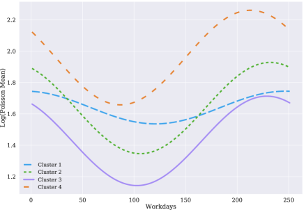
Figure F.1. Cluster-specific arrival rates over time

F.2. Further details on the implementation

We covert all the covariates into z-scores. Since we chose $z_{0}=1$, we set the cost of treatment to $c=4/5309$, where $5309$ is expected number of people arriving in a year, given our Poisson rates (hence, the budget is only sufficient for treating 25% of expected arrivals). Regarding the value-function approximation, we employ the following bases for our main specification:

$$\phi(z,t) =\left(z(1-t),z(1-t)^{2},z^{2}(1-t),z^{2}(1-t)^{2},z\sin(\pi t),\dots\right.$$

$$\qquad\left.\dots,z\sin(2\pi t),z^{2}\sin(\pi t),z^{2}\sin(2\pi t),z^{3}(1-t)\right)^{\intercal}$$

The above specification ensures the basis functions are $0$ when $z=0$ or $t=1$, in line with our boundary condition. When we increase $d_{\nu}$ from 9 to 11 and 13 (in Figure 6.3), we add the terms $\{z^{3}\sin(\pi t),z^{3}\sin(2\pi t)\}$ and $\{z^{3}\sin(\pi t),z^{3}\sin(2\pi t),z^{3}(1-t)^{2},z^{4}(1-t)\}$, respectively.

F.3. Grid search results

Figure F.2 depicts the welfare trajectories for all 27 combinations of tuning parameters from our grid-search. Based on these results, we offer the following conclusions. Low values of $\alpha_{v}$, i.e., $\alpha_{v}=10^{-3}$ in our example, should always be avoided. This is consistent with the theory for Actor-Critic methods, which requires the value parameters to be estimated at fast enough rates. Low values of $\alpha_{\theta}$ (i.e., $\alpha_{\theta}=0.05$) lead to convergence that is too slow. High values of $\alpha_{\theta},\alpha_{v}$ may lead to much faster convergence, but are more volatile in that, under multiple runs, the parameters sometimes become degenerate (i.e., some of the parameters diverge to $\infty$, leading the program to collapse as in the last sub-figure), or only reach a local maximum. This is due to the intrinsic randomness of stochastic gradient descent, which appears to be exacerbated with high learning rates. The plots corresponding to $\{\alpha_{\theta}=50,\alpha_{v}=10^{-2}\}$ and $\{\alpha_{\theta}=5,\alpha_{v}=10^{-1}\}$ suffer from this issue. For instance, we found that under multiple runs, the specification $\{\alpha_{\theta}=50,\alpha_{v}=10^{-2},d_{v}=9\}$ could either perform really well, as it does in this plot, or the parameters could become degenerate (results not shown). In a similar manner, the specification $\{\alpha_{\theta}=5,\alpha_{v}=10^{-1},d_{v}=13\}$ degenerated in the run displayed here, but performed well in other runs (this is also the case with $\{\alpha_{\theta}=50,\alpha_{v}=10^{-2},d_{v}=13\}$, which appears to reach a lower welfare here, but performed similarly to the other $d_{v}$ in other runs). Intermediary learning rates like $\{\alpha_{\theta}=5,\alpha_{v}=10^{-2}\}$ are considerably more stable. It is also possible that this volatility can be substantially reduced by increasing the number of parallel processes (evidence suggesting this is available upon request from the authors). However, for high values of both $\alpha_{\theta},\alpha_{v}$ (i.e., $\alpha_{\theta}=50,\alpha_{v}=10^{-1}$), the parameters degenerated in all cases.

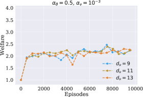
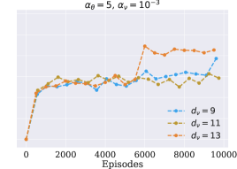
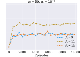
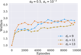
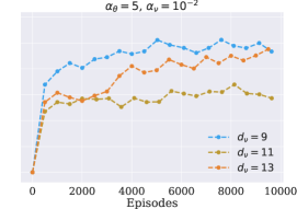
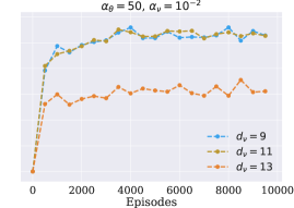
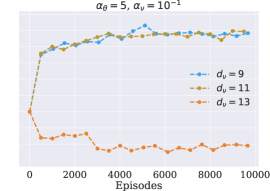
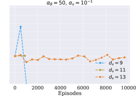
Note: Training was performed in 20 parallel processes. Each point is an average over 500 evaluation episodes. A welfare of $1$ corresponds to a random policy (50% treatment probability). The main specification uses $\alpha_{\theta}=5,\alpha_{\nu}=10^{-2},d_{\nu}=9$.

Figure F.2. Sensitivity to tuning parameters (full grid)

F.4. Benchmark against EWM: Budget Trajectories

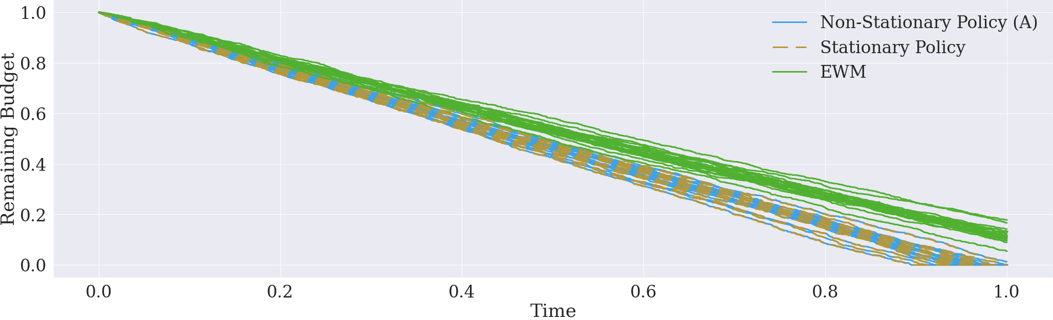
Note: The figure displays results for 20 simulated episodes of the dynamic setting.

Figure F.3. Trajectories of budget over time

Figure F.3 illustrates how our proposed policies do better. It plots the evolution of budget over time under the various policies for 20 simulations of the dynamic setting. The EWM policy consistently leaves some budget unused, a consequence of not taking into account the time constraint. By contrast, both our policies use up all the budget before $t=1$.

Appendix G Properties of viscosity solutions

This section collects various properties of viscosity solutions for the proofs of Theorems 1 and 2. Our first lemma concerns the relationship between the population PDE (2.3) from the main text, and the ‘transformed’ PDE (A.2) introduced in Appendix A. The population PDE (2.3) is given by

(G.1) $$F_{\theta}(z,t,f,Df) =0\ \textrm{on}\ \mathcal{U};\quad\textrm{where},$$

$$F_{\theta}(z,t,u,q_{1},q_{2}) :=\beta u-\lambda(t)\bar{G}_{\theta}(z,t)q_{1}-q_{2}-\lambda(t)\bar{r}_{\theta}(z,t),$$

and $\mathcal{U}$ is some open set. The transformed PDE is given by

(G.2) $$\partial_{\tau}f+H_{\theta}(z,\tau,\partial_{z}f) =0\ \textrm{on}\ \Upsilon;\quad\textrm{where},$$

$$H_{\theta}(z,\tau,p) :=-e^{\beta\tau}\lambda(\tau)\bar{r}_{\theta}(z,\tau)-\lambda(\tau)\bar{G}_{\theta}(z,\tau)p,$$

and $\Upsilon:=\{(z,T-t):(z,t)\in\mathcal{U}\}$. The following lemma shows that there is a one-to-one relationship between the viscosity solutions to these PDEs:

Lemma G.1.

If $u_{\theta}$ is a viscosity solution to (G.2) on $\Upsilon$, then $e^{-\beta(T-t)}u_{\theta}(z,T-t)$ is a viscosity solution to (G.1) on $\mathcal{U}.$ Similarly, if $h_{\theta}$ is a viscosity solution to (G.1) on $\mathcal{U}$, then $e^{\beta\tau}h_{\theta}(z,T-\tau)$ is a viscosity solution to (G.2) on $\Upsilon$.

Proof.

We shall only prove the first claim, as the proof of the other claim is analogous.

Suppose that $u_{\theta}$ is a viscosity solution to (G.2). We will show that $\tilde{h}_{\theta}(z,t):=e^{-\beta(T-t)}u_{\theta}(z,T-t)$ is a viscosity solution to (G.1) on $\mathcal{U}.$ To this end, consider any $\phi\in\mathcal{C}^{2}(\mathcal{U})$ such that $\tilde{h}_{\theta}(z,t)-\phi(z,t)$ attains a local maximum at some $(z^{*},t^{*})\in\mathcal{U}$. It is without loss of generality to suppose that $\tilde{h}_{\theta}(z^{*},t^{*})-\phi(z^{*},t^{*})=0$, as the requirements for a viscosity solution only involve the derivatives of $\phi$ and we can therefore always add or subtract a constant to $\phi$. We then have $e^{\beta(T-t)}\left\{h_{\theta}(z,t)-\phi(z,t)\right\}\leq 0$ for all $(z,t)$ in a neighborhood of $(z^{*},t^{*})$, i.e., $e^{\beta(T-\tau)}\left\{h_{\theta}(z,t)-\phi(z,t)\right\}$ also attains a local maximum at $(z^{*},t^{*})$. This implies $e^{\beta\tau}\left\{h_{\theta}(z,T-\tau)-\phi(z,T-\tau)\right\}$, as a function of $(z,\tau)$, attains a local maximum at $(z^{*},T-t^{*})\in\Upsilon$, or, equivalently, $u_{\theta}(z,\tau)-\tilde{\phi}(z,\tau)$ attains a local maximum at $(z^{*},T-t^{*})\in\Upsilon$, where $\tilde{\phi}(z,\tau):=e^{\beta\tau}\phi(z,T-\tau)$. Since $u_{\theta}$ is a viscosity solution, we thus have

$$\partial_{\tau}\tilde{\phi}(z^{*},T-t^{*})+H_{\theta}(z^{*},T-t^{*},\partial_{z}\tilde{\phi}(z^{*},T-t^{*}))\leq 0,$$

and therefore, after getting rid of a positive multiplicative constant, $e^{\beta(T-t^{*})}$, we get

$$\beta\tilde{h}_{\theta}(z^{*},t^{*})-\lambda(t^{*})\bar{G}_{\theta}(z^{*},t^{*})\partial_{z}\phi(z^{*},t^{*})-\partial_{t}\phi(z^{*},t^{*})-\lambda(t^{*})\bar{r}_{\theta}(z^{*},t^{*})\leq 0,$$

where we have made use of the definitions of $H_{\theta}(\cdot)$ and $\tilde{\phi}(\cdot)$, along with the fact $\tilde{h}_{\theta}(z^{*},t^{*})=\phi(z^{*},t^{*})$. The above implies that $\tilde{h}_{\theta}(z,t)$ is a viscosity sub-solution to PDE (G.1) on $\mathcal{U}$. By an analogous argument, we can similarly show $\tilde{h}_{\theta}(z,t)$ is a viscosity super-solution to PDE (G.1) on $\mathcal{U}$. Hence, $\tilde{h}_{\theta}(z,t):=e^{-\beta(T-t)}u_{\theta}(z,T-t)$ is a viscosity solution to PDE (G.1) on $\mathcal{U}$. ∎

While Lemma G.1 is only stated for the interior domain $\mathcal{U}$, it is straightforward to extend it to the boundary. For the Dirichlet boundary condition, it is easy to verify that if $u_{\theta}=0$ on $\mathcal{B}\equiv\{(z,T-t):(z,t)\in\Gamma\}$, then $\tilde{h}_{\theta}(z,t):=e^{-\beta(T-t)}u_{\theta}(z,T-t)=0$ on $\Gamma$ (an analogous statement also holds for $h_{\theta}$). One can prove similar claims for the Neumann boundary conditions as well, using the same arguments. Hence, the relationship between the viscosity solutions $h_{\theta}(z,t)$ and $u_{\theta}(z,t)$ holds under all the boundary conditions considered in this paper. These results imply that $h_{\theta}$ exists and is unique if and only if $u_{\theta}$ exists and is unique as well.

In the remainder of this section, we collect properties of viscosity solutions broken down into separate cases for each of the boundary conditions:

G.1. Dirichlet boundary condition

Consider the Dirichlet problem for PDEs in Hamiltonian form:

(G.3) $$\partial_{t}f+H\left(z,t,f,\partial_{z}f\right)=0\textrm{ on }\text{$\mathcal{U}$};\quad u=0\textrm{ on }\text{$\Gamma$}.$$

The following comparison theorem is due to Crandall and Lions (1986, Theorem 1). Recall the notation $(f)_{+}:=\max\{f,0\}$.

Theorem G.1.

(Comparison Theorem - Dirichlet form) Suppose that the function $H(\cdot)$ satisfies conditions (R1)-(R3) from Appendix A. Let $u,v$ be respectively, a viscosity sub- and super-solution to

$$\partial_{t}f+H\left(z,t,f,\partial_{z}f\right)=0\textrm{ on }\mathcal{U},$$

where $\mathcal{U}$ is an open set. Then

(G.4) $$\sup_{\bar{\mathcal{U}}}(u-v)_{+}\leq\sup_{\partial\mathcal{U}}(u-v)_{+}.$$

If, alternatively, $\mathcal{U}$ is the of the form $\mathcal{Z}\times(0,T]$, where $\mathcal{Z}$ is any open set, we can replace $\partial\mathcal{U}$ in the statement with $\Gamma\equiv\{\partial\mathcal{Z}\times[0,T]\}\cup\{\mathcal{Z}\times\{0\}\}$.

The above theorem can be applied on any open set $\mathcal{U}$; we do not need to specify the actual boundary condition.

Lemma G.2.

Suppose that Assumptions 1-4 hold for PDE (2.3) under the Dirichlet boundary condition (2.7). Then there exists $L_{0}<\infty$ independent of $\theta,z,t$ such that $|h_{\theta}(z,t)|\leq L_{0}$. In addition, for the setting with $T<\infty$, there exists $K<\infty$ such that $|h_{\theta}(z,t)|\leq K|T-t|$. In a similar vein, for the setting with $\underline{z}>-\infty$, there exists $K_{1}<\infty$ such that $|h_{\theta}(z,t)|\leq K_{1}|z-\underline{z}|$.

Proof.

Consider the Dirichlet problem with $T<\infty$. Define $u_{\theta}(z,\tau):=e^{\beta\tau}h_{\theta}(z,T-\tau).$ Then $u_{\theta}(\cdot)$ is the viscosity solution to (A.2). Now, it is straightforward to verify that $\phi(z,\tau):=K\tau$ is a super-solution to (A.2) as long as $K\geq\sup_{z,\tau}|\lambda(\tau)\bar{r}_{\theta}(z,\tau)|$ (note that $|\lambda(\tau)\bar{r}_{\theta}(z,\tau)|$ is uniformly bounded by virtue of Assumption 2(i)). Hence, by the Comparison Theorem G.1, it follows $u_{\theta}\leq\phi$ on $\bar{\mathcal{U}}$. This implies $u_{\theta}\leq KT$ everywhere, and furthermore, since $h_{\theta}(z,t)=e^{-\beta(T-t)}u_{\theta}(z,T-t)$, that $|h_{\theta}(z,t)|\leq K|T-t|$. A similar argument, after switching the roles of $z,\tau$, also proves $|h_{\theta}(z,t)|\leq K_{1}|z-\underline{z}|$. ∎

Lemma G.3.

Suppose that Assumptions 1-4 hold for PDE (2.3) under the Dirichlet boundary condition (2.7). Then there exists $L_{1}<\infty$ independent of $\theta,z,t$ such that $h_{\theta}(z,t)$ is locally Lipschitz continuous in both arguments with Lipschitz constant $L_{1}$.

Proof.

We consider three cases: (i) $\underline{z}=-\infty$, (ii) $T=\infty$, and (iii) $\underline{z}>-\infty$ and $T<\infty$. For cases (i) and (ii), the claim follows by similar arguments as in Souganidis (1985, Proposition 1.5). For case (iii), the claim follows by similar arguments as in Crandall and Lions (1986, Theorem 4). We refer the reader to the supplementary material for a detailed proof. ∎

G.2. Periodic boundary condition

Consider time-periodic PDEs of the form

(G.5) $$\partial_{t}f+H\left(z,t,f,\partial_{z}f\right) =0\textrm{ on }\text{$\mathcal{U}$};$$

$$f(z,t) =f(z,t+T_{p})\ \forall\ (z,t)\in\mathcal{U}.$$

We first present a stronger version of the Comparison Theorem for Cauchy problems, due to Crandall and Lions (1983). This turns out to be useful to prove a comparison theorem for the periodic problem (G.5).

Lemma G.4.

Suppose $\beta\geq 0$, and the function $H(\cdot)$ satisfies conditions (R1)-(R3) from Appendix A. Let $u,v$ be, respectively, viscosity sub- and super-solutions to

$$\partial_{t}f+H\left(z,t,f,\partial_{z}f\right) =0\ \textrm{on }\mathbb{R}\times(t_{0},\infty).$$

Then for all $t\in[t_{0},\infty)$,

$$e^{\beta(t-t_{0})}\sup_{z\in\mathbb{R}}\left(u(z,t)-v(z,t)\right)_{+}\leq\sup_{z\in\mathbb{R}}\left(u(z,t_{0})-v(z,t_{0})\right)_{+}.$$

Theorem G.2.

(Comparison Theorem - Periodic form) Suppose that the function $H(\cdot)$ satisfies conditions (R1)-(R3) from Appendix A, and that it is $T_{p}$-periodic in $t$. Also suppose that $\beta\geq 0$. Let $u,v$ be respectively, $T_{p}$-periodic viscosity sub- and super-solutions to (G.5) on $\mathcal{U}$. Then $u(x,t)\leq v(x,t)$ on $\mathbb{R}\times\mathbb{R}$.

Proof.

By Lemma G.4, for any $t_{0}\in\mathbb{R},$

$$e^{\beta T_{p}}\sup_{z\in\mathbb{R}}\left(u(z,T_{p}+t_{0})-v(z,T_{p}+t_{0})\right)_{+}\leq\sup_{z\in\mathbb{R}}\left(u(z,t_{0})-v(z,t_{0})\right)_{+}.$$

But by periodicity, $u(z,T_{p}+t_{0})-v(z,T_{p}+t_{0})=u(z,t_{0})-v(z,t_{0})$. Hence,
$\sup_{z\in\mathbb{R}}\left(u(z,t_{0})-v(z,t_{0})\right)_{+}=0$. But the choice of $t_{0}$ was arbitrary; therefore, $u(z,t)\leq v(z,t)$ on $\mathbb{R}\times\mathbb{R}$. ∎

Lemma G.5.

Suppose that Assumptions 1-4 hold for the periodic boundary condition (2.8), and the discount factor $\beta$ is sufficiently large. Then there exists $L_{1}<\infty$ independent of $\theta,z,t$ such that $h_{\theta}$ is locally Lipschitz continuous with Lipschitz constant $L_{1}$.

Proof.

That $h_{\theta}(z,t)$ is Lipschitz continuous in $z$ follows by similar arguments as in Crandall and Lions (1986, Theorem 3). For the Lipschitz continuity of $h_{\theta}(z,t)$ in $t$, we can argue as in Souganidis (1985, Proposition 3.4). We refer the reader to the supplementary material for a detailed proof. ∎

G.3. Neumann boundary condition

For results on the Neumann boundary condition, we impose additional regularity conditions on $H(\cdot)$ and $B(\cdot)$, i.e., in addition to (R1)-(R3) and (R5)-(R8) in Appendices A and B. These are needed to prove Lipschitz continuity of solutions, and are given by (as before, we use the notation $y:=(z,t)$):

• There exist $C_{1},C_{2}<\infty$ such that

  $$\left|H(y_{1},u,p_{1})-H(y_{2},u,p_{2})\right| \leq C_{1}\left(\left\|y_{1}-y_{2}\right\|+\left\|p_{1}-p_{2}\right\|\right),\quad\textrm{and}$$

  $$\left|H(y_{1},u,p)-H(y_{2},u,p)\right| \leq C_{2}\left\|p\right\|\left\|y_{1}-y_{2}\right\|.$$

• There exist $C_{3},C_{4}<\infty$ such that

  $$\left|B(y_{1},u,p_{1})-B(y_{2},u,p_{2})\right| \leq C_{3}\left(\left\|y_{1}-y_{2}\right\|+\left\|p_{1}-p_{2}\right\|\right),\quad\textrm{and}$$

  $$\left|B(y_{1},u,p)-B(y_{2},u,p)\right| \leq C_{4}\left\|p\right\|\left\|y_{1}-y_{2}\right\|.$$

It is straightforward to verify that under Assumptions 1-4, the regularity conditions (R1)-(R3), (R5)-(R8) and (R9)-(R10) are satisfied by $H_{\theta}(\cdot)$ and $B_{\theta}(\cdot)$ in PDE (B.2), with constants $C_{1},C_{2},C_{3}C_{4}$ independent of $\theta$ (this is due to uniform boundedness and Lipschitz continuity of $\lambda(t)$, $\bar{G}_{\theta}(z,t)$ and $\bar{r}_{\theta}(z,t)$ imposed in Assumption 1). The condition (R4) is not required for the results below (it is only used to show existence of a solution). The conditions (R1)-(R3), (R5)-(R8) are also satisfied by $\hat{H}_{\theta}(\cdot)$ in the sample PDE (B.10) under the additional assumption - made is the statement of Theorem 2 - that $G_{a}(x,z,t),\pi_{\theta}(x,z,t)$ are uniformly continuous in $(z,t)$. (R9) and (R10) may not be satisfied by $\hat{H}_{\theta}(\cdot)$. But they are not needed to prove a comparison theorem, being used only to show Lipschitz continuity of solutions, which we do not require for the sample PDE (B.10).

The following results are taken from Barles and Lions (1991), but see also Crandall et al (1992, Theorem 7.12). We refer to those papers for the proofs.

Theorem G.3.

(Comparison Theorem - Neumann form) Suppose that the functions $H(\cdot)$ and $B(\cdot)$ satisfy conditions (R1)-(R3) and (R5)-(R8) in Appendices A and B. Let $u,v$ be respectively, a viscosity sub- and super-solutions to (B.1). Then $u(x,t)\leq v(x,t)$ on $\bar{\mathcal{Z}}\times[0,\bar{T}]$.

Lemma G.6.

Suppose that the functions $H(\cdot)$ and $B(\cdot)$ satisfy conditions (R1)-(R3) and (R5)-(R8) in Appendices A and B, along with (R9)-(R10). Then the unique viscosity solution, $u$, of (B.1) is Lipschitz continuous on $\bar{\mathcal{Z}}\times[0,\bar{T}]$, where the Lipschitz constant depends only on the values of $C_{1}$-$C_{4}$ in (R9)-(R10).

Appendix H Semi-convexity, sup-convolution etc.

In this section, we collect various properties of semi-convex/concave functions, and sup/inf-convolutions used in the proof of Theorem 1. Since the results are well-known in the literature, we will only state them here. The interested reader is referred to the supplementary material for the proofs.

H.1. Semi-convexity and concavity

In what follows, we take $y$ to be a vector in $\mathbb{R}^{d}$. Moreover, for any vector $y$, $|y|$ denotes its Euclidean norm.

Definition 3.

A function $u$ on $\mathbb{R}^{d}$ is said to be semi-convex with the coefficient $c$ if $u(y)+\frac{c}{2}|y|^{2}$ is a convex function. Similarly, $u$ is said to be semi-concave with the coefficient $c$ if $u(y)-\frac{c}{2}|y|^{2}$ is concave.

Lemma H.1.

Suppose that $u$ is semi-convex. Then $u$ is twice differentiable almost everywhere. Furthermore, at every point $y$ for which $Du$ exists,

$$u(y+h)\geq u(y)+h^{\intercal}Du(y)-\frac{c}{2}|h|^{2}\ \ \forall\ h\in\mathbb{R}^{d}.$$

An analogous property also holds for semi-concave functions. We can also extend the scope of the theorem to points where $Du$ does not exist by considering one-sided derivatives, which can be shown to exist everywhere for semi-convex functions.

H.2. Sup and Inf Convolutions

Let $u(y)$ denote a continuous function on some open set $\mathcal{Y}$. Let $\partial\mathcal{Y}$ denote the boundary of $\mathcal{Y}$, and $\bar{\mathcal{Y}}$ its closure. Also, $\left\|Du\right\|$ denotes the Lipschitz constant for $u$, with the convention that it is $\infty$ if $u$ is not Lipschitz continuous.

Definition 4.

The function $u^{\epsilon}$ is said to be the sup-convolution of $u$ if

$$u^{\epsilon}(y)=\sup_{\tilde{y}\in\mathcal{\bar{Y}}}\left\{u(\tilde{y})-\frac{1}{2\epsilon}|\tilde{y}-y|^{2}\right\}.$$

Similarly, $u_{\epsilon}$ is said to be the inf-convolution of $u$ if

$$u_{\epsilon}(y)=\inf_{\tilde{y}\in\bar{\mathcal{Y}}}\left\{u(\tilde{y})+\frac{1}{2\epsilon}|\tilde{y}-y|^{2}\right\}.$$

The following lemma characterizes the properties of sup-convolutions (similar results apply for inf-convolutions):

Lemma H.2.

Suppose that $u$ is continuous on $\bar{\mathcal{Y}}$. Then,

(i) $u^{\epsilon}$ is semi-convex with coefficient $1/\epsilon$.

(ii) For all $y\in\bar{\mathcal{Y}}$, $|u^{\epsilon}(y)-u(y)|\leq 4\left\|Du\right\|^{2}\epsilon$.

(iii) $\left\|Du^{\epsilon}\right\|\leq 4\left\|Du\right\|.$

Our next lemma concerns PDEs of the form

$$F(y,u(y),Du(y))=0\textrm{ on }\mathcal{\mathcal{Y}}.$$

We assume that $F(\cdot)$ satisfies the following property:

(H.1) $$|F(y_{1},q_{1},p)-F(y_{2},q_{2},p)|\leq C|p|\{|q_{1}-q_{2}|+|y_{1}-y_{2}|\},$$

where $C<\infty$ is some constant. Define $\mathcal{Y}_{\epsilon}$ as the set of all points in $\mathcal{Y}$ that are at least $2\left\|Du\right\|\epsilon$ distance away from $\partial\mathcal{Y},$ i.e.,

$$\mathcal{Y}_{\epsilon}:=\{y\in\mathcal{Y}:|y-w|>2\left\|Du\right\|\epsilon\ \forall\ w\in\partial\mathcal{Y}\}.$$

Lemma H.3.

Suppose that $u$ is a viscosity solution to $F(y,u,Du)=0$ on $\mathcal{Y}$, and $\left\|Du\right\|\leq m<\infty$. Suppose also that $F(\cdot)$ satisfies (H.1). Then, there exists some $c$ depending on only $C$ (from H.1) and $m$ such that $F(y,u^{\epsilon},Du^{\epsilon})\leq c\epsilon$ in the viscosity sense for all $y\in\mathcal{Y}_{\epsilon}$.

References

- Achdou et al., (2017) Achdou, Y., Han, J., Lasry, J.-M., Lions, P.-L., and Moll, B. (2017). Income and wealth distribution in macroeconomics: A continuous-time approach. Technical report, National Bureau of Economic Research.
- Adusumilli, (2021) Adusumilli, K. (2021). Risk and optimal policies in bandit experiments. arXiv preprint arXiv:2112.06363.
- Anderberg, (1973) Anderberg, M. R. (1973). Cluster Analysis for Applications. Academic Press, New York.
- Athey and Wager, (2018) Athey, S. and Wager, S. (2018). Efficient Policy Learning. arXiv:1702.02896.
- Barles and Chasseigne, (2014) Barles, G. and Chasseigne, E. (2014). (almost) everything you always wanted to know about deterministic control problems in stratified domains. arXiv preprint arXiv:1412.7556.
- Barles and Lions, (1991) Barles, G. and Lions, P.-L. (1991). Fully nonlinear neumann type boundary conditions for first-order hamilton–jacobi equations. Nonlinear Analysis: Theory, Methods & Applications, 16(2):143–153.
- Benitez-Silva et al., (2000) Benitez-Silva, H., Hall, G., Hitsch, G. J., Pauletto, G., and Rust, J. (2000). A comparison of discrete and parametric approximation methods for continuous-state dynamic programming problems. manuscript, Yale University.
- Bhatnagar et al., (2009) Bhatnagar, S., Sutton, R. S., Ghavamzadeh, M., and Lee, M. (2009). Natural Actor-Critic Algorithms. Automatica, 45(11):2471–2482.
- Bhattacharya and Dupas, (2012) Bhattacharya, D. and Dupas, P. (2012). Inferring Welfare Maximizing Treatment Assignment under Budget Constraints. Journal of Econometrics, 167:168–196.
- Bostan and Namah, (2007) Bostan, M. and Namah, G. (2007). Time periodic viscosity solutions of hamilton-jacobi equations. In Applied Analysis And Differential Equations, pages 21–30. World Scientific.
- Brockman et al., (2016) Brockman, G., Cheung, V., Pettersson, L., Schneider, J., Schulman, J., Tang, J., and Zaremba, W. (2016). Openai gym. arXiv preprint arXiv:1606.01540.
- Chamberlain, (2011) Chamberlain, G. (2011). Bayesian Aspects of Treatment Choice. In Geweke, J., Koop, G., and Van Dijk, H., editors, The Oxford Handbook of Bayesian Econometrics, pages 11–39. Oxford University Press.
- Chernozhukov et al., (2018) Chernozhukov, V., Chetverikov, D., Demirer, M., Duflo, E., Hansen, C., Newey, W., and Robins, J. (2018). Double/debiased machine learning for treatment and structural parameters. The Econometrics Journal, 21(1):C1–C68.
- Crandall, (1997) Crandall, M. G. (1997). Viscosity solutions: a primer. In Viscosity solutions and applications, pages 1–43. Springer.
- Crandall et al., (1984) Crandall, M. G., Evans, L. C., and Lions, P.-L. (1984). Some properties of viscosity solutions of hamilton-jacobi equations. Transactions of the American Mathematical Society, 282(2):487–502.
- Crandall et al., (1992) Crandall, M. G., Ishii, H., and Lions, P.-L. (1992). User’s guide to viscosity solutions of second order partial differential equations. Bulletin of the American mathematical society, 27(1):1–67.
- Crandall and Lions, (1983) Crandall, M. G. and Lions, P.-L. (1983). Viscosity solutions of hamilton-jacobi equations. Transactions of the American mathematical society, 277(1):1–42.
- Crandall and Lions, (1986) Crandall, M. G. and Lions, P.-L. (1986). On existence and uniqueness of solutions of hamilton-jacobi equations. Nonlinear Analysis: Theory, Methods & Applications, 10(4):353–370.
- Degrave et al., (2022) Degrave, J., Felici, F., Buchli, J., Neunert, M., Tracey, B., Carpanese, F., Ewalds, T., Hafner, R., Abdolmaleki, A., de Las Casas, D., et al. (2022). Magnetic control of tokamak plasmas through deep reinforcement learning. Nature, 602(7897):414–419.
- Fan and Glynn, (2021) Fan, L. and Glynn, P. W. (2021). Diffusion approximations for thompson sampling. arXiv preprint arXiv:2105.09232.
- Hirano and Porter, (2009) Hirano, K. and Porter, J. R. (2009). Asymptotics for Statistical Treatment Rules. Econometrica, 77(5):1683–1701.
- Ishii, (1985) Ishii, H. (1985). Hamilton-jacobi equations with discontinuous hamiltonians on arbitrary open sets. Bull. Fac. Sci. Eng. Chuo Univ, 28(28):1985.
- Kidambi et al., (2020) Kidambi, R., Rajeswaran, A., Netrapalli, P., and Joachims, T. (2020). Morel: Model-based offline reinforcement learning. arXiv preprint arXiv:2005.05951.
- Kitagawa and Tetenov, (2018) Kitagawa, T. and Tetenov, A. (2018). Who Should Be Treated? Empirical Welfare Maximization Methods for Treatment Choice. Econometrica, 86(2):591–616.
- Kock et al., (2018) Kock, A. B., Preinerstorfer, D., and Veliyev, B. (2018). Functional sequential treatment allocation. arXiv preprint arXiv:1812.09408.
- Laber et al., (2014) Laber, E. B., Lizotte, D. J., Qian, M., Pelham, W. E., and Murphy, S. A. (2014). Dynamic treatment regimes: Technical challenges and applications. Electronic journal of statistics, 8(1):1225.
- Mandt et al., (2017) Mandt, S., Hoffman, M. D., and Blei, D. M. (2017). Stochastic gradient descent as approximate bayesian inference. The Journal of Machine Learning Research, 18(1):4873–4907.
- Manski, (2004) Manski, C. F. (2004). Statistical Treatment Rules for Heterogeneous Populations. Econometrica, 72(4):1221–1246.
- Mnih et al., (2016) Mnih, V., Badia, A. P., Mirza, M., Graves, A., Lillicrap, T., Harley, T., Silver, D., and Kavukcuoglu, K. (2016). Asynchronous methods for deep reinforcement learning. In International conference on machine learning, pages 1928–1937.
- Mnih et al., (2015) Mnih, V., Kavukcuoglu, K., Silver, D., Rusu, A. A., Veness, J., Bellemare, M. G., Graves, A., Riedmiller, M., Fidjeland, A. K., Ostrovski, G., Petersen, S., Beattie, C., Sadik, A., Antonoglou, I., King, H., Kumaran, D., Wierstra, D., Legg, S., and Hassabis, D. (2015). Human-Level Control through Deep Reinforcement Learning. Nature, 518(7540):529–533.
- Silver et al., (2018) Silver, D., Hubert, T., Schrittwieser, J., Antonoglou, I., Lai, M., Guez, A., Lanctot, M., Sifre, L., Kumaran, D., Graepel, T., Lillicrap, T., Simonyan, K., and Hassabis, D. (2018). A general reinforcement learning algorithm that masters chess, shogi, and go through self-play. Science, 362(6419):1140–1144.
- Silver et al., (2017) Silver, D., Schrittwieser, J., Simonyan, K., Antonoglou, I., Huang, A., Guez, A., Hubert, T., Baker, L., Lai, M., Bolton, A., et al. (2017). Mastering the game of go without human knowledge. Nature, 550(7676):354.
- Slivkins, (2019) Slivkins, A. (2019). Introduction to multi-armed bandits. arXiv preprint arXiv:1904.07272.
- Souganidis, (1985) Souganidis, P. E. (1985). Existence of viscosity solutions of hamilton-jacobi equations. Journal of Differential Equations, 56(3):345–390.
- Souganidis, (2009) Souganidis, P. E. (2009). Rates of convergence for monotone approximations of viscosity solutions of fully nonlinear uniformly elliptic pde (viscosity solutions of differential equations and related topics).
- Stoye, (2009) Stoye, J. (2009). Minimax Regret Treatment Choice with Finite Samples. Journal of Econometrics, 151(1):70–81.
- Sutton and Barto, (2018) Sutton, R. S. and Barto, A. G. (2018). Reinforcement learning: An introduction. MIT press.
- Sutton et al., (2000) Sutton, R. S., McAllester, D. A., Singh, S. P., and Mansour, Y. (2000). Policy gradient methods for reinforcement learning with function approximation. In Advances in neural information processing systems, pages 1057–1063.
- Tetenov, (2012) Tetenov, A. (2012). Statistical treatment choice based on asymmetric minimax regret criteria. Journal of Econometrics, 166(1):157–165.
- Tsitsiklis and Van Roy, (1997) Tsitsiklis, J. and Van Roy, B. (1997). An analysis of temporal-difference learning with function approximation. IEEE Transactions on Automatic Control, 42(5):674–690.
- Wager and Xu, (2021) Wager, S. and Xu, K. (2021). Diffusion asymptotics for sequential experiments. arXiv preprint arXiv:2101.09855.
- Yu et al., (2020) Yu, T., Thomas, G., Yu, L., Ermon, S., Zou, J., Levine, S., Finn, C., and Ma, T. (2020). Mopo: Model-based offline policy optimization. arXiv preprint arXiv:2005.13239.