Effects of the QCD Equation of State and Lepton Asymmetry on Primordial Gravitational Waves

Abstract

Using the quantum chromodynamics (QCD) equation of state (EoS) from lattice calculations we investigate effects from QCD on primordial gravitational waves (PGWs) produced during the inflationary era. We also consider different cases for vanishing and nonvanishing lepton asymmetry where the latter one is constrained by cosmic microwave background experiments. Our results show that there is up to a few percent deviation in the predicted gravitational wave background in the frequency range around the QCD transition ($10^{-10}-10^{-7}$ Hz) for different lattice QCD EoSs, or at larger frequencies for nonvanishing lepton asymmetry using perturbative QCD. Future gravitational wave experiments with high enough sensitivity in the measurement of the amplitude of PGWs like SKA, EPTA, DECIGO and LISA can probe these differences and can shed light on the real nature of the cosmic QCD transition and the existence of a nonvanishing lepton asymmetry in the early universe.

I Introduction

The era of observing the universe beyond electromagnetic waves began by the first gravitational wave (GW) observation of LIGO produced from two merging black holes Abbott et al. (2016). This gives the opportunity to probe phenomena in astrophysics and cosmology which are impossible or difficult to be observed by photons. The inflationary scenario has been proposed in cosmology as a solution to the flatness, the horizon, and magnetic monopole problems Linde (1982); Guth (1981). It was shown that inflation can also produce primordial gravitational waves (PGWs) as the tensor perturbation of the metric of spacetime Starobinsky (1979). This also opens up a direct way to check the physics of the early universe before big bang nucleosynthesis (BBN) which until now has been hidden from our sight except for its possible effects on the cosmic microwave background Seljak and Zaldarriaga (1997); Lyth (1997); Spergel et al. (2007); Ade et al. (2016). Different phenomena like electroweak transition, QCD transition, phase transition in the dark sector, early matter domination, etc., can be present before BBN which can produce extra GWs or affect PGWs produced by the inflationary scenario Schwarz (1998); Maggiore (2000); Mazumdar and White (2018).

The equation of state (EoS) of the standard model (SM) can have different impacts on PGWs due to possible features coming from the quark–gluon and the electroweak transitions Schwarz (1998); Maggiore (2000); Mazumdar and White (2018). These effects can be measured by future GW experiments. There are some ongoing and future space and earth based GW detectors like DECIGO Seto et al. (2001); Sato et al. (2017), LISA Audley et al. (2017), SKA Janssen et al. (2015), and EPTA Lentati et al. (2015), which can measure the possible effects of cosmic (phase) transitions in the visible and dark side of the universe in the relevant frequency ranges.

The thermal effect of the SM on PGWs appears via the trace anomaly and the energy and entropy density of radiation in the equation of motion for PGWs produced from inflation. The trace anomaly of the energy momentum tensor of the SM shows deviations of the EoS from pure radiation (with $p=\rho/3$) which are due to quantum effects and the nonrelativistic behavior of SM particles at temperatures below about one third of their masses Schwarz (1998); Watanabe and Komatsu (2006); Schettler et al. (2011); Caprini and Figueroa (2018). Effects from the trace anomaly in the SM are most pronounced at the QCD transition Aoki et al. (2006).

The QCD transition can affect the cosmology of the early universe in different aspects like its effect on the relic density of dark matter and the GW spectrum Drees et al. (2015); Schwarz (1998); Castorina et al. (2018); Anand et al. (2017); Schwarz (2003); Stuke et al. (2012); Saikawa and Shirai (2018); Hindmarsh and Philipsen (2005); Borsanyi et al. (2016); Capozziello et al. (2019); Li et al. (2018). What we know from lattice QCD calculations at vanishing chemical potentials for baryon, electric charge, and strangeness number is that the QCD transition is a smooth crossover Aoki et al. (2006). This is in contrast to first studies on the QCD phase diagram for the early universe which adopted a first order or second order phase transition Witten (1984); Asakawa and Yazaki (1989). However, the effect of considering nonvanishing chemical potentials can slightly change the strength of the transition and lead to different EoSs compared to the case of vanishing chemical potentials Schwarz and Stuke (2009); Stuke et al. (2012).

In the present study we focus on the imprints of QCD on PGWs for the cases of vanishing and nonvanishing lepton flavor asymmetry in the early universe. This paper is organized as follows. In section II we outline our formalism to compute the relic PGW spectrum and the relevant thermodynamic relations. Then we discuss the impact of different QCD EoSs, based on different lattice QCD results, on the PGW spectrum in section III paying special attention to effects from the charm quark contribution. Effects on PGWs from nonvanishing chemical potentials, in particular from a nonvanishing lepton asymmetry, are discussed in section IV. Finally, we conclude in section V.

II Primordial Gravitational Waves from Inflation

The production of GWs by the inflationary scenario in the early universe can be considered by doing a perturbative analysis of the Friedmann equations. In standard cosmology the following metric describes the evolution of the cosmos assuming vanishing curvature which is a reasonable assumption for an isotropic and homogeneous universe Dodelson (2003) and matches with observations Ade et al. (2016):

$$ds^{2}=-dt^{2}+a(t)^{2}d{\bf{x}}^{2}\,,$$ (1)

where the relation between the cosmic time $t$ and the conformal time $\eta$ can be defined by $dt=a\,d\eta$. The tensor perturbation equation in the Fourier space which shows the evolution of PGWs is given by Dodelson (2003)

$$h^{{}^{\prime\prime}}(k,\eta)+2\mathcal{H}(\eta)h^{{}^{\prime}}(k,\eta)+k^{2}h(k,\eta)=0\,,$$ (2)

where ${}^{\prime}\coloneqq d/d\eta$. The conformal Hubble rate is denoted by $\mathcal{H}=a^{\prime}/a=aH$. By using $v(k,\eta)=a(\eta)h(k,\eta)$ one has

$$v^{{}^{\prime\prime}}(k,\eta)+\left(k^{2}-\frac{a^{{}^{\prime\prime}}}{a}\right)v(k,\eta)=0\,,$$ (3)

with

$$\frac{a^{{}^{\prime\prime}}}{a}=\frac{4\pi G}{3}\left(\rho_{\rm{tot}}-3p_{\rm{tot}}\right)\,,$$ (4)

where $8\pi G=1/M_{\rm{Pl}}^{2}$ and $M_{\rm{Pl}}=1.22\times 10^{19}$ GeV. The quantity in the parentheses at the right hand side of eq. (4) is called the trace anomaly (or interaction measure) and can be written as follows Cheng et al. (2008); Bazavov et al. (2014a, 2017)

$$\frac{I(T)}{T^{4}}=\frac{\rho_{\rm{tot}}-3p_{\rm{tot}}}{T^{4}}=T\frac{\partial}{\partial T}\left(\frac{p_{\rm{tot}}}{T^{4}}\right)_{\mu/T}\,.$$ (5)

In eq. (4) one should consider the total energy and pressure density with respect to the scale factor taking into account entropy conservation in the early universe. The entropy density $s_{\rm{tot}}$ can be derived by using thermodynamic relations which we show below. For this one needs also the Friedmann equation which reads

$$H^{2}=\frac{8\pi G}{3}\rho_{\rm{tot}}\,.$$ (6)

At any specific time, $t(\eta)$, during the cosmic evolution super horizon modes can be defined for $k\eta\ll 1$. When the universe expands and modes enter the horizon, they are identified as sub horizon modes by $k\eta\gg 1$. The frequency of each mode $k$ can be written as $f=k/2\pi$. The initial condition for modes outside the horizon that we used to solve eq. (3) to compute the GW spectrum are Dodelson (2003); Schettler et al. (2011)

$$v(k,\eta_{\rm{ini}}) = \frac{1}{k^{3/2}}\,,$$

$$v^{\prime}(k,\eta_{\rm{ini}}) = \frac{v(k,\eta_{\rm{ini}})}{r_{\rm{ini}}}\,,\quad r_{\rm{ini}}~{}=~{}\frac{1}{a(\eta_{\rm{ini}})H(\eta_{\rm{ini}})}\,,$$ (7)

where the oscillatory factor of the wave function, $\exp(ik\eta)$, is neglected, as it only affects the phase of the GW, not the amplitude we are interested in. In choosing these initial conditions only the $k$ dependence is important for our purpose.

By assuming entropy conservation during the QCD transition and until today, one can compute the evolution of $\rho_{\rm{tot}}(a)$ by solving eq. (6) backward in time, i.e. from today ($a_{0}=1$) to a chosen scale factor $a$ in the early universe . Then the solution can be used to solve eq. (3).

Due to the large range of the scale factor from today ($a_{0}=1$) back to the early universe when we consider modes well before horizon crossing (temperatures well above the electroweak transition) numerical problems for solving the differential equation given by eq. (3) might arise. Therefore, one solves the differential equation either until horizon crossing for each mode or until a temperature after neutrino decoupling to include all the evolution of the EoS in the calculation. In practice both of these ways of calculating the GW spectrum will give approximately the same final result. Since the slight change of the EoS due to the change of trace anomaly happens in a short interval of the scale factor with a tiny deviation from the radiation-like EoS, this will cause a tiny change in the amplitude of the GW when the mode enters the horizon until the end of neutrino decoupling. This procedure is sufficient for our goal to show the effects from QCD and from a lepton asymmetry on PGWs. We also check the difference between two procedures in a specific frequency ($3\times 10^{-11}$ and $5\times 10^{-8}$ Hz) range such that we can find the numerical solution in a precise way. Definitely, if one finds any evidence of PGWs in experiments a more detailed calculation can be done by fixing the scale of inflation from the data to have a more precise handle on the aforementioned effects to match theory with experiment.

For each polarization mode ($\lambda$) of the GW eq. (2) is valid and the amplitude of perturbations can be written as Caprini and Figueroa (2018)

$$h_{\lambda}(k,\eta)=h_{\lambda}^{\rm{prim}}(k)Y(\eta,k)=\frac{v(k,\eta)}{a(\eta)}\,,$$ (8)

then the energy density of GWs is given by Caprini and Figueroa (2018); Watanabe and Komatsu (2006)

$$\rho_{\rm{GW}}(\eta)=\frac{M_{\rm{Pl}}^{2}}{32\pi a(\eta)^{2}}\left<h_{ij}^{\prime}(k,{\bf x})h^{ij\prime}(k,{\bf x})\right>\,,$$ (9)

$$\left<h^{\prime}_{ij}(k,{\bf x})h^{ij\prime}(k,{\bf x})\right>=\int\frac{dk}{k}\mathcal{P}_{T}(k,\eta)\,.$$ (10)

The tensor power spectrum is defined by

$$\mathcal{P}_{T}(k,\eta) = \frac{k^{3}}{\pi^{2}}\sum_{\lambda}\left<|h_{\lambda}(k,\eta)|^{2}\right>$$ (11)

$$= \mathcal{P}^{\rm{prim}}_{T}(k)[Y(k,\eta)]^{2}\,,$$

where its time independent part reads

$$\mathcal{P}^{\rm{prim}}_{T}(k)=\frac{k^{3}}{\pi^{2}}\sum_{\lambda}\left<|h^{\rm{prim}}_{\lambda}(k)|^{2}\right>=\frac{1}{\pi}\left(\frac{4H_{\rm{inf}}}{M_{\rm{Pl}}}\right)^{2}\,.$$ (12)

The Hubble parameter at the inflation scale is fixed by $H_{\rm{inf}}^{2}\approx(8\pi/3M_{Pl}^{2})V_{\rm{inf}}$. The relic density of GWs can be obtained by

$$\Omega_{\rm{GW}}(k,\eta)=\frac{\mathcal{P}^{\rm{prim}}_{T}(k)}{12a(\eta)^{2}H(\eta)^{2}}[Y^{\prime}(k,\eta)]^{2}\,.$$ (13)

Equations (12) and (13) show that the absolute value of the relic density of PGWs depends on the inflationary scale. Assuming an inflationary scale of $V_{\rm inf}^{1/4}=1.5\times 10^{16}$ GeV the relic density of GWs for the frequency range between $10^{-9}$–$10^{-10}$ Hz will be $\Omega_{\rm{GW}}h^{2}\sim 2.4\times 10^{-16}$ Saikawa and Shirai (2018).

At the horizon it can be found that $[Y^{\prime}(k,\eta)]^{2}=k^{2}[Y(k,\eta)]^{2}$. This can change when modes come well inside the horizon Watanabe and Komatsu (2006); Saikawa and Shirai (2018). Since our goal is to evaluate the effect of the EoS on the PGWs and to compare their relic amplitude at high frequency to their relic amplitude at low frequency, using eqs. (8), (12), and (13), we can write

$$\Omega_{\rm{GW}}(k,\eta_{0})\propto\Omega_{\rm{GW}}(k,\eta_{\rm{hc}})\propto k^{5}|v(k,\eta_{\rm{hc}})|^{2}\,,$$ (14)

where the horizon crossing mode can be identified by

$$k=a(\eta_{\rm{hc}})H(\eta_{\rm{hc}})\,.$$ (15)

The temperature at horizon crossing can also be determined by using eqs. (6) and (15). One can also find the following approximate relation between PGW relic, energy, and entropy density at horizon crossing Schwarz (1998); Watanabe and Komatsu (2006); Saikawa and Shirai (2018)

$$\Omega_{\rm{GW}}(k,\eta_{0})\propto\rho_{\rm{tot}}(T_{hc})s_{\rm{tot}}(T_{\rm{hc}})^{-4/3}\,.$$ (16)

We can solve eqs. (3), (4), and (6) with the initial conditions given by eq. (II) until the scale factor at horizon reaches a value where each mode $k$ crosses the horizon or until a scale factor at lower temperatures, e.g., after neutrino decoupling. After neutrino decoupling, since the GWs evolve like radiation ($\rho_{\rm{GW}}\propto a^{-4}$) in case of the absence of any phase transition afterwards, the spectrum will be unchanged until today except for the damping in the amplitude due to the expansion. This helps us to pin down the relative difference of PGWs for different modes due to the evolution of the EoS with temperature in the early universe. We do not consider the effect of an anisotropic stress due to the free streaming of photons and decoupled neutrinos, which appears as a source on the right hand side of eq. (2), because it is effective only for frequencies smaller than $\sim 5\times 10^{-11}$ Hz Weinberg (2004); Watanabe and Komatsu (2006); Saikawa and Shirai (2018).

III The Role of the Equation of State of the SM on PGWs

In order to solve eq. (3) for different GW wave numbers $k$ it is required to first solve eqs. (4) and (6) to find the temperature as a function of $a$ or $\eta$. For this purpose, we should know the quantities $\rho_{\rm{tot}}$ and $p_{\rm{tot}}$ at each temperature $T$. The total energy and pressure density can be computed from the following equations

$$\rho_{\rm{tot}}(T,\mu) = \sum_{i}\frac{g_{i}}{2\pi^{2}}\int_{m_{i}}^{\infty}dE\times$$ (17)

$$E^{2}\sqrt{E^{2}-m_{i}^{2}}\left(\frac{1}{e^{\frac{E-\mu_{i}}{T}}\pm 1}\right)\,,$$

$$p_{\rm{tot}}(T,\mu) = \sum_{i}\frac{g_{i}}{6\pi^{2}}\int_{m_{i}}^{\infty}dE\times$$ (18)

$$\left(E^{2}-m_{i}^{2}\right)^{3/2}\left(\frac{1}{e^{\frac{E-\mu_{i}}{T}}\pm 1}\right)\,,$$

with the sum over all particle species $i$ with degrees of freedom $g_{i}$ and chemical potential $\mu_{i}$. The total entropy density is given by

$$Ts_{\rm{tot}}(T,\mu) = \rho_{\rm{tot}}(T,\mu)+p_{\rm{tot}}(T,\mu)$$ (19)

$$-\sum_{i}\mu_{i}n_{i}(T,\mu_{i}),$$

For each particle species the net number density of particles minus anti–particles can be defined as

$$n_{i}(T,\mu_{i}) = \frac{g_{i}}{2\pi^{2}}\int_{m_{i}}^{\infty}dE~{}E\sqrt{E^{2}-m_{i}^{2}}\times$$ (20)

$$\left(\frac{1}{e^{\frac{E-\mu_{i}}{T}}\pm 1}-\frac{1}{e^{\frac{E+\mu_{i}}{T}}\pm 1}\right)\,.$$

The above equations can be used to determine the energy and entropy density of the SM which can be implemented in eqs. (3), (4), and (6) to compute the relic density of PGW in the early universe according to eq. (13).

In this section we only consider the case of vanishing chemical potentials. Several studies have been performed before for the case of vanishing chemical potentials using different lattice QCD results around the QCD transition available at that time Borsanyi et al. (2016); Laine and Schroder (2006); Drees et al. (2015); Laine and Meyer (2015); Saikawa and Shirai (2018); Hindmarsh and Philipsen (2005) and considering different assumptions for the EoS in the perturbative regime of QCD, at the electroweak transition, and for neutrino decoupling.

As shown in refs. Schettler et al. (2011); Saikawa and Shirai (2018) the characteristic frequency of PGWs related to the QCD transition temperature, $T_{\rm{QCD}}\sim 150$ MeV, is $f_{\rm{QCD}}\approx 3\times 10^{-9}$ Hz. The effect of neutrino decoupling at low temperature ($T\sim 1$ MeV and $f\sim 10^{-11}$ Hz) is important to compute the precise value of temperature with respect to the scale factor Lesgourgues and Pastor (2012). This effect appears due to the varying temperatures of different neutrino flavors during and after neutrino decoupling Lesgourgues and Pastor (2012).

Figure 1: The trace anomaly including lattice QCD results for temperatures up to $500$ MeV taken from different approaches Laine and Meyer (2015); Saikawa and Shirai (2018); Drees et al. (2015); Borsanyi et al. (2016). See text for details.

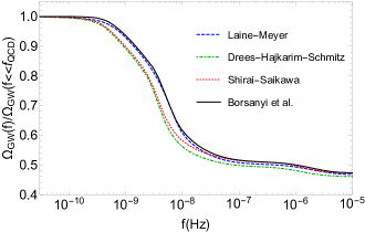
Figure 2: The PGW spectrum with respect to frequency using different EoSs for the early universe shown in the previous figure.

The main QCD EoS we use is the one by ref. Borsanyi et al. (2016) (labeled as ‘Borsanyi et al.’ in the figures). In ref. Borsanyi et al. (2016) the EoS from $10$ MeV to ($500$ MeV) $1$ GeV for ($2+1$) $2+1+1$ flavors by using lattice methods is computed. Their computed trace anomaly for all SM particles and the predicted PGW spectrum are shown in fig. 1 and 2, respectively. By using hard thermal loop corrections and the perturbative QCD approach up to order $\mathcal{O}(g_{s}^{6})$ including effects from charm and bottom quarks, they derive the EoS for temperatures above $1$ GeV Andersen et al. (2011); Kajantie et al. (2003). They use the results of ref. Laine and Meyer (2015) for very high temperatures around the electroweak transition. For smaller temperatures they adopt a hadron resonance gas (HRG) model approach Huovinen and Petreczky (2010). Thereby they provide the EoS for temperatures between $1$ MeV and $100$ GeV including all SM particles. The data set of ref. Borsanyi et al. (2016) is the one we use to extract the impact of charm quarks from lattice QCD calculations on PGWs.

In fig. 1 and fig. 2 the corresponding result of Drees et al. (2015) for the QCD EoS of the standard model is shown using the data of the HotQCD Collaboration Bazavov et al. (2014a) for $2+1$ flavors and the EoS including also charm quark by ref. Borsanyi et al. (2010). Also, the HRG model data is used for temperatures between $70$ and $100$ MeV Huovinen and Petreczky (2010). The remaining SM particles are assumed to be free particles. Moreover, the effect of neutrino decoupling has been considered using ref. Lesgourgues and Pastor (2012). The interpolated result for the EoS of ref. Bazavov et al. (2017), using another lattice calculation for vanishing chemical potentials, highly matches the result of Bazavov et al. (2014a) in the temperature range of $130-230$ MeV, so that we do not include their results in this paper.

Additionally, we compare the thermal evolution of the EoS of the SM with a calculation by Laine and Meyer Laine and Meyer (2015) who used the older treatment of Laine and Schroeder Laine and Schroder (2006) for temperatures below $110$ GeV. In ref. Laine and Schroder (2006) the radiative corrections up to order $\mathcal{O}(g_{s}^{2})$ for a running quark mass are considered. For temperatures below $350$ MeV old lattice data for pure glue theory is used. The EoS of ref. Laine and Schroder (2006) includes temperatures between $10$ MeV and $1$ TeV including all SM particles. However, since the mass of the Higgs boson was unknown at that time, they have considered a different value from the nowadays accepted one. This issue is fixed in the work of Laine and Mayer Laine and Meyer (2015) by considering $125$ GeV for the Higgs mass and including corrections from lattice field theory calculations around the electroweak transition ($110$ GeV$\lesssim T\lesssim 250$ GeV). For temperatures above $250$ GeV they have considered the perturbative result of Gynther and Vepsalainen (2006). The result for their treatment for the trace anomaly up to a temperature of $500$ MeV is shown in fig. 1. The comparison of the influence of the EoS of Laine and Meyer on the PGW spectrum with the other EoSs for the early universe is shown in fig. 2.

Another treatment of the SM EoS that we investigate is from the work of ref. Saikawa and Shirai (2018) which used lattice QCD results for $2+1+1$ flavors Borsanyi et al. (2016) matched to a HRG model Huovinen and Petreczky (2010) at temperatures below the QCD transition and perturbative QCD up to $\mathcal{O}(g_{s}^{6}\log g_{s})$ at higher temperatures Kajantie et al. (2003). For temperatures around the electroweak transition the results of refs. Laine and Meyer (2015); D’Onofrio and Rummukainen (2016); Buttazzo et al. (2013) considering lattice calculations and perturbative calculations are used. At very low temperatures around electron and neutrino decoupling the result of de Salas and Pastor (2016) is adopted to consider the effect of neutrino oscillations. The effect of this EoS on the trace anomaly, PGW and the differences compared to result obtained with the EoS of ref. Borsanyi et al. (2016) are shown in figs. 1 and 2, respectively.

In fig. 1 results for the trace anomaly of QCD based on different lattice calculations reported in the literature are shown. It can be seen that the location of the peak in the trace anomaly is similar but the height differs for different approaches as different input from lattice calculations have been used. Figure 2 shows the effect of using the different results for the trace anomaly on the relic density of PGWs as a function of the frequency. For frequencies in the range $10^{-10}-10^{-9}$ Hz ($T\sim 10-100$ MeV for horizon crossing) the HRG model and muons play the major role for the PGW relic density. For frequencies between $10^{-9}$ and $10^{-7}$ Hz the EoS including lattice QCD results, tau leptons and bottom quarks are important for determining the GW relic density for horizon crossing temperatures between $100$ MeV and $10$ GeV. For temperatures around $100$ GeV and frequencies around $10^{-6}$ Hz the appearance of top quarks and the electroweak sector including W^±, Z, and Higgs bosons have the dominant impact on the SM EoS and the prediction of the stochastic GW background.

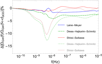
Figure 3: The relative differences of the predicted relic density of PGWs using the EoSs from refs. Laine and Meyer (2015); Saikawa and Shirai (2018); Drees et al. (2015) compared to the one of ref. Borsanyi et al. (2016). The opaque curves do not include the effect of electron and neutrino decoupling to better compare the role of QCD on the relic density of PGWs with the main data set Borsanyi et al. (2016). The transparent curves include the contribution due to electron and neutrino decoupling.

Two of the EoSs Drees et al. (2015); Saikawa and Shirai (2018) shown in fig. 2 consider effects from neutrino decoupling but this effect is not taken into account for the other EoSs Borsanyi et al. (2016); Laine and Meyer (2015). Neutrino decoupling leads to a shift of the PGW spectrum to higher frequencies compared to the case without considering neutrino decoupling taken into account. Moreover, it causes a relative error of up to $\sim 10$% between two cases as shown in fig. 3. The discrepancy originates mainly from the change in determining the precise relation between the scale factor and the temperature using eqs. (4) and (6) which differs if one takes into account neutrino decoupling or not. The differences in the trace anomaly (shown in fig. 1), energy, and entropy density are mostly due to the various treatments of the QCD EoS. As fig. 3 shows using different EoSs results in a deviation of up to $3-4$% at frequencies around $3\times 10^{-9}$ Hz and up to $3$% for higher frequencies if one neglects the effect from neutrino decoupling. The deviations in the predicted PGW relic shown in fig. 2 are computed at the scale factor of horizon crossing for each mode which is numerically doable. We also studied the deviations for a limited frequency range ($3\times 10^{-11}$ and $5\times 10^{-8}$ Hz) at a fixed scale factor after neutrino decoupling when the evolution of the EoS will not be affected by SM particles any more. Our results show that highly evolving the EoS especially around the QCD transition improve the predicted PGW relic around $1$%, since the deviation of the EoS from radiation causes a small damping of PGWs after horizon crossing. We do not show the plot for this calculation in this paper, since our frequency range is limited and doing it for a larger frequency range is numerically expensive. These discrepancies between different treatments of the EoS can be distinguished by SKA, EPTA, LISA, and DECIGO at different frequencies by the observation of PGWs.

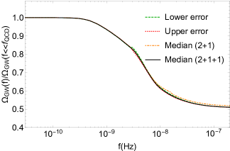
Figure 4: The error band of the relic density of PGWs from median value ($2+1+1$) by taking the lower and upper bounds from lattice data of ref. Borsanyi et al. (2016). Also, the effect of including charm quarks in lattice simulations on the he relic density is presented using the data of ref. Borsanyi et al. (2016) for $2+1$ and $2+1+1$ flavors for the median values. As it can be seen there is a deviation between the computed relic density of PGWs due to charm quarks mostly for frequencies around $10^{-8}$ Hz and higher.

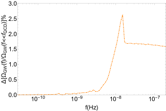
Figure 5: The error due to the effect of charm quarks at low temperatures in lattice simulations on PGWs is presented using the data of ref. Borsanyi et al. (2016) for $2+1$ and $2+1+1$ flavors.

In fig. 4 the effect of considering charm quarks in lattice calculations on the predicted relic density of PGWs is shown using lattice data from ref. Borsanyi et al. (2016) for $2+1$ and $2+1+1$ flavors. The difference is small but not negligible. The relative difference of the predicted pattern of PGWs between $2+1$ and $2+1+1$ flavors in lattice QCD for different frequencies is shown in fig. 5 and amounts up to $2.6$%. For frequencies higher than $2\times 10^{-8}$ Hz the difference is due to the change in the relation between energy density and scale factor computed from eq. 6, since a lower temperature as an initial condition affects this relation for the higher temperature.

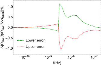
Figure 6: The relative error on the relic density of PGWs due to the uncertainties in the EoS from lattice QCD and perturbative calculations from ref. Borsanyi et al. (2016).

We also consider the uncertainties of the lattice data and the perturbative QCD calculations up to $\mathcal{O}(g_{s}^{6})$ for the temperature range of $100$ MeV to $10$ GeV considering $2+1+1+1$ flavors, i.e., including effects from bottom quarks, which is discussed in ref. Borsanyi et al. (2016). The resulting error band in the relic density of PGWs is depicted in fig. 4. One sees that the changes are small. In fact, the relative error in the relic density of PGWs amounts to a discrepancy of at most $1.1$% around the QCD transition as shown in fig. 6.

IV SM with Nonvanishing Chemical Potentials and PGWs

The value of the lepton asymmetry in the universe is constrained by analyses of BBN and the cosmic microwave background (CMB) to be Oldengott and Schwarz (2017):

$$l=\frac{n_{L}}{s}\lesssim 0.012\,.$$ (21)

Also from the Planck data Aghanim et al. (2018) one knows the amount of baryon asymmetry of the universe

$$b=\frac{n_{B}}{s}\approx 8\times 10^{-11}\,.$$ (22)

Considering SM particles in a thermal bath and assuming that sphaleron processes occur efficiently then the lepton asymmetry is related to the baryon asymmetry by $l=-\frac{51}{28}b$ Harvey and Turner (1990). Such tiny values for the lepton asymmetry and baryon asymmetry do not lead to a first order phase transition of QCD Wygas et al. (2018); Bazavov et al. (2018). However, such a small value of $l$ has not been confirmed experimentally. The effect of a sizable lepton asymmetry on the evolution of the chemical potentials of SM particles with respect to temperature and its effect on the cosmic trajectory has been investigated in refs. Schwarz and Stuke (2009); Wygas et al. (2018).

In the early universe, between neutrino oscillations ($T_{\rm{osc}}\sim 10$ MeV) and the electroweak transition ($T_{\rm{ew}}\sim 100$ GeV), conservation of nonvanishing lepton flavor asymmetries, baryon asymmetry, and electric charge leads to the following set of equations Schwarz and Stuke (2009); Wygas et al. (2018):

$$l_{f}s(T,\mu) = n_{f}(T,\mu_{f})+n_{\nu_{f}}(T,\mu_{\nu_{f}})\,,f=e,\mu,\tau\,,$$

$$bs(T,\mu) = \sum_{i}b_{i}n_{i}(T,\mu_{i})\,,$$

$$0 = \sum_{i}{q_{i}n_{i}(T,\mu_{i})}\,,$$ (23)

with $n_{i}$ is the net number density of particles minus anti-particles given by eq. (20) and we presumed electric charge neutrality of the universe in the last equation.

The total entropy density can be determined according to eq. (19) using eqs. (17) and (18) considering all relevant SM particles and their chemical potentials. Solving this system of coupled equations at a given temperature we get the temperature evolution of the SM chemical potentials Wygas et al. (2018) and thus we can compute the total pressure and energy density for nonvanishing lepton asymmetries (cf. Wygas (2018)). For the numerical evaluation we assumed equally distributed lepton flavor asymmetries, $l_{f}=l/3$.

For different temperature ranges one can find approximate relations between the lepton flavor chemical potentials and the electric charge chemical potential. For example in the temperature range where lattice QCD plays a major role, i.e., $150$ MeV$<T<350$ MeV (the upper bound is defined due to the presence of charm quarks at higher temperatures) we have $\mu_{Q}\approx\mu_{l_{f}}/2$. For temperatures between the QCD transition and the temperature where pions are not relativistic anymore ($m_{\pi^{\pm}}/3<T<150$ MeV) one finds $\mu_{Q}\approx 2\mu_{l_{f}}/3$. For even lower temperatures but above neutrino decoupling one can find $\mu_{Q}\approx\mu_{l_{f}}$ due to charge conservation Schwarz and Stuke (2009); Wygas et al. (2018); Gebhardt (2018).

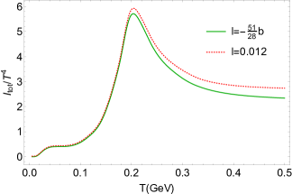
Figure 7: The trace anomaly for vanishing and nonvanishing lepton asymmetry.

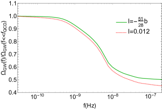
Figure 8: The scaled relic density of PGWs versus frequency assuming different values for the lepton asymmetry.

To calculate the influence of a nonvanishing lepton asymmetry on PGWs one needs the temperature evolution of the energy and entropy density at nonvanishing lepton asymmetry for the early universe. We calculate the EoS between 150 MeV and 350 MeV according to ref. Wygas et al. (2018); Wygas (2018) using lattice QCD susceptibilities ($\chi_{ab}=(\partial^{2}p/\partial\mu_{a}\partial\mu_{b})|_{\mu=0}$) Bazavov et al. (2014b); Mukherjee et al. (2016) to determine the evolution of the chemical potentials at nonvanishing lepton asymmetry. The hadron resonance gas model (HRG) is computed by using a similar approach as in Huovinen and Petreczky (2010) for temperatures below $100$ MeV by considering hadrons up to a mass of $2.5$ GeV as an ideal gas. The energy and entropy density at nonvanishing chemical potentials for temperatures above 350 MeV are calculated as described before according to Wygas et al. (2018), using the results of Laine and Schroder (2006) for considering perturbative QCD effects up to order $\mathcal{O}(g_{s}^{2})$ in case of vanishing chemical potentials.

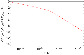
Figure 9: The relative change of the relic density of PGWs due to the presence of nonvanishing lepton chemical potentials for the SM in the thermal bath of the early universe using the data of fig. 8.

Figures 7 and 8 show the trace anomaly and the relic density of PGWs for different values of the lepton asymmetry in the early universe, respectively. There is up to a $10$% difference between considering nearly vanishing ($l=-\frac{51}{28}b$) and nonvanishing lepton asymmetry ($l=0.012$, $l_{e}=l_{\mu}=l_{\tau}=0.004$). This result is based on the computation at horizon crossing. We also checked it with the calculation at a specific scale factor after neutrino decoupling and found the difference between these two methods to be less than $1$%. Here we used the EoS calculated according to Wygas (2018) in the PGWs relic density for frequencies above $\sim 10^{-11}$ Hz. A deviation of the EoS from the predicted value for vanishing lepton asymmetry can be measured in the spectrum of PGWs for frequencies around $10^{-9}-10^{-6}$ Hz by SKA or EPTA, at higher frequencies $10^{-5}-10^{-2}$ Hz by LISA (this frequency range is outside the range plotted in fig. 9), or at $10^{-3}-1$ Hz by DECIGO. The detection of a sizeable lepton asymmetry in the early universe can give impetus for possible scenarios for the explanation of the matter-antimatter asymmetry in the early universe and today. We would like to emphasize that such a small deviation in the EoS of the SM from a vanishing lepton asymmetry can not be observed by CMB measurements, since its presence mostly shows up before BBN when more SM particles are present in the thermal bath.

V Summary and Conclusions

In this paper we studied the effect of the QCD EoS using different lattice QCD simulations including vanishing and nonvanishing chemical potentials Bazavov et al. (2014a); Laine and Meyer (2015); Borsanyi et al. (2010, 2016); Wygas et al. (2018) on the relic density of PGWs produced by the inflationary scenario. These kind of GWs can be observed by different experiments at a level of less than $1$% in the relic density per frequency depending on the length of observation and the sensitivity Seto et al. (2001); Sato et al. (2017); Audley et al. (2017); Janssen et al. (2015); Lentati et al. (2015). The SKA and EPTA experiments are designed for frequencies $10^{-9}-10^{-6}$ Hz by measuring the variation in the distance of pulsars. SKA can observe the PGW background relic density for values as small as $\Omega_{\rm{GW}}h^{2}\approx 10^{-16}$ depending on the time of exposure which is at the order of few decades. Other experiments like LISA and DECIGO which are proposed for larger frequencies $10^{-5}-1$ Hz can also probe the QCD effects mostly due to perturbative effects on the EoS of the SM at higher temperatures.

Different sets for the EoS from refs. Laine and Meyer (2015); Saikawa and Shirai (2018); Drees et al. (2015); Borsanyi et al. (2016) have been used to calculate the PGW spectrum. The difference between the various EoSs of the SM, using different lattice QCD data as input, results in a relative difference of up to $4$% (fig. 3) in the relic density of PGWs, mostly between frequencies of $10^{-9}-10^{-8}$ Hz and somewhat smaller differences at higher frequencies. We also considered the uncertainties of the EoS given in Borsanyi et al. (2016) by taking lower and upper error bounds of lattice QCD calculations into account which leads to a deviation of up to $1.1$% (fig. 6) in the relic density of PGWs in the frequency range of $10^{-9}-10^{-7}$ Hz. Additionally, we investigated the effect of considering charm quarks using lattice QCD data at temperatures lower than $1$ GeV which causes up to $2.6$% deviation in the predicted PGW density around a frequency of $10^{-8}$ Hz (fig. 5).

We also discussed the effect of a nonvanishing lepton asymmetry on the EoS of matter in the early universe. Our calculation shows that this can lead to a difference of up to $2-10$% in the relic density of PGWs for frequencies around and larger than $f_{\rm{QCD}}\sim 3\times 10^{-9}$ Hz (fig. 8). Observing such a deviation from the standard PGW relic density at vanishing lepton asymmetry will elucidate and shed new light on possible solutions for the existence of the baryon asymmetry of the universe.

Finally, based on our current knowledge of the QCD phase diagram, the presence of uncertainties in lattice simulations and our ignorance about the properties of the quark gluon plasma in the early universe we do not have a unique and confirmed picture about the real nature of QCD at early eras. The observation of stochastic GWs produced by inflation may illuminate these issues and deepen our understanding about the EoS of matter before BBN. The structure of the QCD phase can also be changed due to nonvanishing isospin chemical potential of charged pions or other SM particles and may lead to pion condensation Abuki et al. (2009); Brandt et al. (2018) which might affect the thermal history of the universe and also the PGWs. We leave this investigation for future work.