Edge states of a three dimensional kicked rotor

Abstract

Edge localization is a fascinating quantum phenomenon. In this paper, the underlying mechanism generating it is presented analytically and verified numerically for a weakly kicked three-dimensional rotor. Analogy to tight binding model in solid state physics is used. The edge states result of the edge at zero angular momentum of the three-dimensional kicked rotor.

Technion - Israel Institute of Technology, Technion City, Haifa 3200004, Israel

1 Introduction

Edge state localization is a fascinating quantum phenomenon and has been explored extensively in various fields. Edge states have been studied analytically and experimentally in photonic crystals [1, 2], semiconductors [3, 4] and topological insulators [5, 6, 7]. In this paper, we study the edge states in angular momentum space for a three-dimensional kicked rotor [8, 9, 10], a paradigm system for studying quantum effects in a classically chaotic system [11]. This system was numerically and experimentally realized with planar molecules kicked by periodic short microwave [12] and laser [8, 9, 13] pulses. The formation of the edge states was studied numerically [14] for such a system excited at a fractional quantum resonance. In this regime, the period of kicks is a rational fraction of the natural period of the rotor [15].

The regime of quantum resonance [15, 16] has no analog in classical physics. In this regime, the energy of the rotor grows quadratically with the number of kicks, since an initial wavefunction explores higher angular momentum states as time progresses. [10]. However, since the angular momentum quantum number cannot be negative in our system, it creates quasienergy edge states, similar to the states on the surface of a crystal. These states, centered near zero angular momentum, do not acquire energy as time progresses.

In this paper, the mechanicm for creation of such states, resulting of broken translational invariance symmetry, is presented. It uses the fact that the $z$ component of angular momentum (in the standard coordinate system) is zero. The translational invariance in angular momentum is broken near in the vicinity of zero angular momentum. In particular, we show that the wave number becomes imaginary, resulting in exponential decay of such states. In the derivation we use perturbation theory in order to understand in great detail the mechanism for creation of the edge states. We believe that this mechanism is relevant also in the non-perturbative regime, where some of the experiments are performed [8, 9, 10, 12, 13, 14].

The system studied here is described by the Hamiltonian

$$H^{\prime}=\frac{\hbar^{2}}{2I}l\left(l+1\right)+\overline{P}\cos\left(\theta\right)\sum_{m=1}^{\infty}\delta\left(t^{\prime}-mT^{\prime}\right),$$ (1)

where $I$ is the moment of intertia, $\overline{P}$ the kick strength, $T^{\prime}$ the period of the kicks and $\theta$ the planar angle of the rotor. In dimensionless units $t=\frac{t^{\prime}}{T^{\prime}}$ , $H=\frac{H^{\prime}T^{\prime}}{\hbar},$ $\tau=\frac{\hbar T^{\prime}}{I}$ and $P=\frac{\overline{P}}{\hbar},$ this Hamiltonian becomes

$$H=\frac{1}{2}\tau l\left(l+1\right)+P\cos\left(\theta\right)\sum_{m=1}^{\infty}\delta\left(t-m\right).$$ (2)

Note that $\tau$ is the ratio between the driving period and the natural period of the rotor [17]. Here, we are looking at a rotor model where $m=0$.

In this paper, we aim to show analytically the creation of an edge state in a regime of a fractional quantum resonance, therefore, $\tau$ has to be a rational fraction of $4\pi.$ For this purpose, we have chosen

$$\tau=\frac{4\pi}{3}.$$ (3)

In order to describe the propagation of an initial wavefunction in time, we write a transfer matrix $T$ which propagates the wavefunction one kick forward in time

$$T\psi\left(t\right)=\psi\left(t+T\right).$$ (4)

We write this matrix as a product of two matrices

$$T=T_{kin}\cdot T_{P},$$ (5)

where the kinetic and kick parts are

$$T_{kin}=e^{-i\frac{\tau}{2}l\left(l+1\right)}$$ (6)

and

$$T_{P}=e^{-iP\cos\left(\theta\right)},$$ (7)

respectively.

For this value of $\tau$, the kinetic part of the transfer matrix (6) is periodic with period 3. The quasienergies of the matrix $T_{kin}$ are

$$E_{1}=1$$ (8)

and

$$E_{2}=\alpha,$$ (9)

where

$$\alpha=e^{i\frac{2\pi}{3}},$$ (10)

and $E_{1}$ is doubly degenerate. This degeneracy is lifted when a correction to these energies due to the kicks is calculated.

For a free three-dimensional rotor, its eigenfunctions are spherical harmonics, and $T_{P}$ is, for $m=0$ [8],

$$T_{P,ll^{\prime}} =\left\langle l,0\right|e^{-iP\cos\left(\theta\right)}\left|l^{\prime},0\right\rangle$$ (11)

$$=\frac{\sqrt{\left(2l+1\right)\left(2l^{\prime}+1\right)}}{2}\int_{0}^{\pi}P_{l}\left(\cos\left(\theta\right)\right)P_{l^{\prime}}\left(\cos\left(\theta\right)\right)e^{-iP\cos\left(\theta\right)}\sin\left(\theta\right)d\theta,$$

where $P_{l}\left(\cos\left(\theta\right)\right)$ are Legendre polynomials. Detailed discussion is found in Appendix A.

We approximate the transfer matrix for weak kicking strength $P$ and large values of $l$ up to $P^{3}$ as

$$T=\begin{pmatrix}.&.&.&.&.&.&.&.&.\\ .&.&\alpha A&\alpha B&\alpha C&\alpha D&0&.&.\\ .&.&B&A&B&C&D&0&.\\ .&.&C&B&A&B&C&D&0\\ .&.&\alpha D&\alpha C&\alpha B&\alpha A&\alpha B&\alpha C&\alpha D\\ .&.&0&D&C&B&A&B&C\\ .&.&.&0&D&C&B&A&B\\ .&.&.&.&.&.&.&.&.\end{pmatrix},$$ (12)

where

$$A \simeq 1-\frac{P^{2}}{4}$$ (13)

$$B \simeq -i\frac{P}{2}+i\frac{P^{3}}{16}$$ (14)

$$C \simeq -\frac{P^{2}}{8}$$ (15)

and

$$D\simeq i\frac{P^{3}}{48}.$$ (16)

The calculation can be found in Appendix A. This approximation holds for large values of $l,$ far from the edge. We use the matrix (12) in further calculations due to its periodicity. The correction for smaller values of $l$ will manifest itself in the energy of the edge state.

The transfer matrix (12) is periodic, therefore in further calculations we use a solid state tight binding system as an analog. This analog between a solid state tight binding model [18, 19, 20, 21] and a periodically kicked system is a convenient one, and was first proposed in 1982 by Grempel, Fishman and Prange [22].

The paper is organized as follows. In Sect. 2 the solid state analog of the transfer matrix is presented. In Sect. 3 the quasienergies of a weakly kicked rotor are approximated using perturbation theory. In Sect. 4 the quasienergy and wavenumber of the edge state are calculated and compared to the numerical results. The results are summarized and discussed in Sect. 5.

2 Solid state tight binding analog of the transfer matrix

Since the transfer matrix (12) is periodic with period three, we use an analog of a solid state system with three atoms in a unit cell. The eigenvectors of such a system are

$$\phi=\sqrt{\frac{3}{N}}\sum_{l^{\prime}}\left(\alpha_{1}e^{ik\cdot\left(3l^{\prime}\right)}+\alpha_{2}e^{ik\cdot\left(3l^{\prime}+1\right)}+\alpha_{3}e^{ik\cdot\left(3l^{\prime}+2\right)}\right).$$ (17)

where $N$ is the number of atoms in the crystal, $k$ is the wavenumber and $\alpha_{1},\alpha_{2}$ and $\alpha_{3}$ are constants.

We therefore rewrite the transfer matrix as

$$T_{solid}=\begin{pmatrix}\alpha A+\alpha D\left(e^{3ik}+e^{-3ik}\right)&\alpha Be^{ik}+\alpha Ce^{-2ik}&\alpha Be^{-ik}+\alpha Ce^{2ik}\\ Be^{-ik}+Ce^{2ik}&A+D\left(e^{3ik}+e^{-3ik}\right)&Be^{ik}+Ce^{-2ik}\\ Be^{ik}+Ce^{-2ik}&Be^{-ik}+Ce^{2ik}&A+D\left(e^{3ik}+e^{-3ik}\right)\end{pmatrix}.$$ (18)

A detailed calculation is found in Appendix B.

3 Calculating the quasienergies using perturbation theory

The eigenvalues of the matrix (18) are of the form $E=\exp\left(i\omega\right),$ where $\omega$ are the quasienergies of the rotor. After calculating $\det\left(T_{solid}-I\cdot E\right)$ and equating to zero, the following characteristic equation for the energies is obtained

$$E^{3}-E^{2}\left(1-\frac{P^{2}}{4}+i\frac{P^{3}}{48}\gamma\right)\left(\alpha+2\right)$$ (19)

$$-E\Bigg{(}\left(2\alpha+1\right)\left(-1+\frac{P^{2}}{4}\right)+\alpha i\frac{P^{3}}{24}\gamma+i\frac{P^{3}}{48}\gamma\Bigg{)}-\alpha = 0$$

Using (19), we calculate the correction to (8) and (9) for small $P$ using perturbation theory. The resulting energies are, up to the third order in $P,$

$$E_{1}\simeq 1\pm i\frac{1}{2}P+\frac{3\left(1+\alpha^{*}\right)\gamma-12\alpha^{*}}{48\left(\alpha^{*}-1\right)}P^{2}$$ (20)

and

$$E_{20}\simeq\alpha+\frac{\left(\alpha+1\right)}{4\left(\alpha^{*}-1\right)}P^{2}-\frac{iP^{3}\alpha\gamma}{48},$$ (21)

where

$$\gamma=e^{-3ik}+e^{3ik}.$$ (22)

Detailed calculation can be found in Appendix B.

Comparison between the numerical quasienergies for a three-dimensional rotor and a theoretical result from (20) is shown in Fig. 1. The edge state appears at $k=0$ and its theoretical quasienergy is given by (29). Note that the edge state energy does not appear in the theoretical graph, because the calculation was made for a periodic matrix, which fits the transfer matrix for large values of $l,$ far from $l=0.$

Eq. (20) yields the following dispersion relation

$$\gamma=\frac{16\left(\alpha^{*}-1\right)}{\left(\alpha^{*}+1\right)P^{2}}\left(E+\frac{iP}{2}-1\right)+\frac{4\alpha^{*}}{1+\alpha^{*}}$$ (23)

4 Edge state formation

The edge state in a three-dimensional rotor system is formed at $l=0$, where $l$ stands for angular momentum, because only its non-negative values are allowed. This edge results in an eigenstate centered around $l=0$ and whose decay is a function of the imaginary part of the wavenumber $k.$

4.1 Calculating $E_{edge}$

We calculate the quasienergy of the edge state as an eigenvalue of a $2\times 2$ matrix $T_{0}$ that is a subset of the transfer matrix $T$ close to $T_{00}$

$$T_{0}=\begin{pmatrix}T_{00}&T_{01}\\ T_{10}&T_{11}\end{pmatrix},$$ (24)

this is because although the edge state is centered around $l=0,$ it has a “tail” which involves $l=1.$ In this matrix (24) we also take into account the correction for small $l.$ Using (11) yields

$$T_{0}=\begin{pmatrix}T_{00}&T_{01}\\ \alpha T_{01}&T_{11}\end{pmatrix},$$ (25)

where

$$T_{00} =1-\frac{P^{2}}{6},$$ (26)

$$T_{01} =-\frac{iP}{\sqrt{3}}+\frac{iP^{3}}{10\sqrt{3}}$$ (27)

and

$$T_{11}=\alpha\left(1-\frac{3P^{2}}{10}\right),$$ (28)

respectively.

The energy of the edge state is one of the eigenvalues of (24) and it is, up to $P^{3},$

$$E_{edge}=\frac{1}{2}\left(1+\alpha-P^{2}\cdot\frac{5+9\alpha}{30}+\sqrt{\left(1-\alpha\right)^{2}-\frac{P^{2}}{15}\left(9\alpha^{2}+6\alpha+5\right)}\right).$$ (29)

A detailed calculation is found in Appendix C. This energy is shown in Fig. 1 for $P=0.3$ and $P=1.$

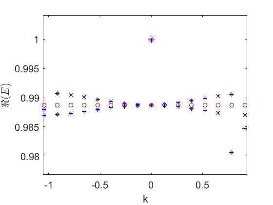
(a)

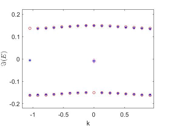
(b)

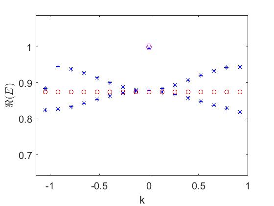
(c)

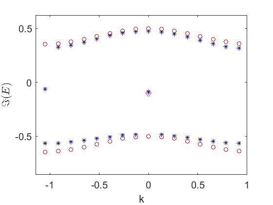
(d)

Figure 1: Comparison between the real and imaginary parts of the quasienergy numerically found using the transfer matrix (5) for a three-dimensional kicked rotor and a theoretical result (21) for $\tau=4\pi/3$ and $P=0.3$ ((a),(b)) and $P=1$ ((c),(d)). The numerical result is shown by asterisks, the theoretical result based on (2) is shown by circles and the theoretical energy of the edge state (29) is shown by a diamond.

4.2 Calculating $k_{edge}$

In order to calculate the wavenumber corresponding to (29), we substitute (29) into (23) and use

$$k_{1,2}=\frac{i}{3}\ln\left(\frac{\gamma_{edge}}{2}\pm\sqrt{\frac{\gamma_{edge}^{2}}{4}-1}\right)$$ (30)

where

$$\gamma_{edge}=e^{3ik_{edge}}+e^{-3ik_{edge}}.$$ (31)

The absolute value of the edge state $\psi_{edge}$ as function of $l$ is shown in Fig. 2 below. Notice that it is large at zero angular momentum.

Since $k_{edge}$ has an imaginary part, it causes the corresponding state to decay exponentially as function of $l.$ Hence, the absolute value of the edge state can be approximated as

$$\left|\psi_{edge}\right|\varpropto e^{-\text{$\Im\left(k_{edge}\right)$}l}.$$ (32)

The comparison between the absolute value of the edge state and a model state with this decay rate is shown in Fig. 2 for $P=0.3$ and $P=1$. The logarithm of $\left|\psi_{edge}\right|$ is compared to the theoretical slope according to (32) in Fig. 3.

We repeated the calculation for $P=2$ and $P=3$ and found considerable deviation from the numerical result for the energies. However, the edge states presented reasonable agreement with the numerical results.

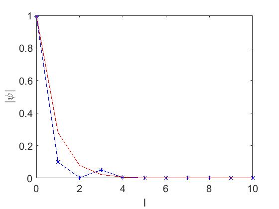
(a)

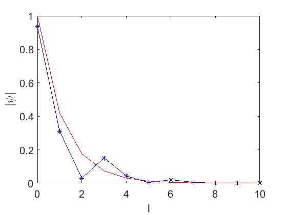
(b)

Figure 2: Comparison between the quasienergy state$\left|\psi_{edge}\right|$ found numerically using the transfer matrix (5)and $\left|\psi_{edge}\right|$ of (32) for (a) $P=0.3$, (b) $P=1$ and $\tau=4\pi/3$ for a three dimensional kicked rotor. The numerical result is shown by asterisks and the theoretical result by a continuous line.

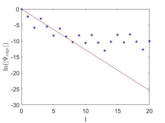
(a)

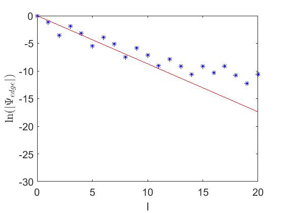
(b)

Figure 3: Comparison between the logarithm of the quasienergy state $\ln\left|\psi_{edge}\right|$ found numerically using the Hamiltonian (2) and $\ln\left|\psi_{edge}\right|$ of (32) for (a) $P=0.3$, (b) $P=1$ and $\tau=4\pi/3$ for a three dimensional kicked rotor. The numerical result is shown by asterisks and the theoretical result by a continuous line.

5 Summary and discussion

In a three-dimensional rotor system studied here, edge states appear due to the edge in angular momentum at $l=0$ (see Eq. (11)). An initial wavevector located near $l$=0 will stay there as time progresses. Near this region, the transfer matrix (12) becomes dependent on $l$ while for large values of $l$ it is similar to the two dimensional rotor matrix (and independent of $l$).

We analytically calculated the energy and decay rate of the edge states for the three dimensional rotor system using an analog tight binding model, based on the periodicity of the transfer matrix. The energy of the edge state was found along with its exponential decay rate, and a comparison between the theoretical and numerical results was shown in Figs. 2 and 3. In this paper, it was demonstrated analytically in great detail how edge states in angular momentum, that were found numerically in the past [14], are generated. We calculated the edge states also for $P=2$ and $P=3$ and found reasonable agreement with the numerical results. Therfore, we believe this mechanism is valid also in the non-perturbative regime, where most experiments are done [8, 9, 10, 12, 13, 14]. This result is expected to motivate future research, in particular of the non-perturbative regime.

Author contribution statement

All authors contributed equally to the research and presentation in the paper.

Appendix A Transfer matrix calculation for three-dimensional rotor

In order to calculate the transfer matrix elements for the three dimensional rotor, we use the fact that for $m=0$ the spherical harmonics can be written using Legendre polynomials as

$$Y_{\theta}^{0}=\sqrt{\frac{2l+1}{4\pi}}P_{l}\left(\cos\left(\theta\right)\right),$$ (A.1)

where $P_{l}$ are Legendre polynomials. We also use the following formula for integration of Legendre polynomials [23]

$$\int_{-1}^{1}P_{k}\left(x\right)P_{l}\left(x\right)P_{m}\left(x\right)dx=2\begin{pmatrix}k&l&m\\ 0&0&0\end{pmatrix}^{2}$$ (A.2)

where

$$\begin{pmatrix}k&l&m\\ 0&0&0\end{pmatrix}=\left(-1\right)^{s}\sqrt{\frac{\left(2s-2k\right)!\left(2s-2l\right)!\left(2s-2m\right)!}{\text{$\left(2s+1\right)$!}}}\cdot\frac{s!}{\left(s-k\right)!\left(s-l\right)!\left(s-m\right)!}$$ (A.3)

for $2s$ even, and zero otherwise, where

$$2s=k+l+m,$$ (A.4)

and calculate the integrals corresponding to each diagonal up to the third diagonals to the right and left (since the calculation is up to $P^{3}$) , using the relation

$$\cos^{3}\left(\theta\right)=\frac{3}{5}P_{1}\left(\cos\left(\theta\right)\right)+\frac{2}{5}P_{3}\left(\cos\left(\theta\right)\right).$$ (A.5)

For example, for the main diagonal we have

$$\left\langle l,0\right|e^{-iP\cos\left(\theta\right)}\left|l,0\right\rangle \simeq\left\langle l,0\right|1-iP\cos\left(\theta\right)-\frac{P^{2}}{2}\cos^{2}\left(\theta\right)+\frac{i}{6}P^{3}\cos^{3}\left(\theta\right)\left|l,0\right\rangle$$ (A.6)

We know that

$$-iP\left\langle l,0\right|\cos\left(\theta\right)\left|l,0\right\rangle =-iP\frac{2l+1}{2}\int_{0}^{\pi}P_{l}^{2}\left(\cos\left(\theta\right)\right)\cos\left(\theta\right)\sin\left(\theta\right)d\theta$$ (A.7)

$$=-iP\frac{2l+1}{2}\int_{-1}^{1}P_{l}^{2}\left(x\right)xdx=0$$

because in the integral we have an antisymmetric function integrated over a symmetric interval.

The integral for $P^{2}$ yields

$$-\frac{P^{2}}{4}\left(2l+1\right)\int_{0}^{\pi}P_{l}^{2}\left(\cos\left(\theta\right)\right)\cos^{2}\left(\theta\right)\sin\left(\theta\right)d\theta =-\frac{P^{2}}{4}\left(2l+1\right)\int_{-1}^{1}P_{l}^{2}\left(x\right)x^{2}dx$$ (A.8)

$$=-\frac{P^{2}}{2}\frac{2l^{2}+2l-1}{\left(2l-1\right)\left(2l+3\right)}$$

and the integral for $P^{3}$ yields, using (A.5) and (A.2),

$$\frac{iP^{3}}{6}\int_{-1}^{1}P_{l}^{2}\left(x\right)x^{3}dx =\frac{iP^{3}}{10}\int_{-1}^{1}P_{l}^{2}\left(x\right)P_{1}\left(x\right)dx+\frac{iP^{3}}{15}\int_{-1}^{1}P_{l}^{2}\left(x\right)P_{3}\left(x\right)dx$$ (A.9)

$$=\frac{iP^{3}}{5}\begin{pmatrix}l&l&1\\ 0&0&0\end{pmatrix}^{2}+\frac{2iP^{3}}{15}\begin{pmatrix}l&l&3\\ 0&0&0\end{pmatrix}^{2}=0$$

because $2s$ is odd in both expressions.

The results for each diagonal are as follows. For the main diagonal the result is

$$T_{main}=1-\frac{P^{2}}{2}\cdot\frac{2l^{2}+2l-1}{\left(2l-1\right)\left(2l+3\right)}.$$ (A.10)

For the first diagonal to the right and left it is

$$T_{1st,right}=-iP\cdot\frac{l+1}{\sqrt{\left(2l+1\right)\left(2l+3\right)}}+\frac{iP^{3}}{20}\left[\frac{2l+2}{\sqrt{\left(2l+1\right)\left(2l+3\right)}}+\frac{l\left(2l+2\right)\left(l+2\right)}{\left(2l-1\right)\left(2l+5\right)\sqrt{\left(2l+1\right)\left(2l+3\right)}}\right]$$ (A.11)

and

$$T_{1st,left}=-iP\cdot\frac{l}{\sqrt{\left(2l+1\right)\left(2l-1\right)}}+i\frac{P^{3}}{20\sqrt{\left(2l+1\right)\left(2l-1\right)}}.\left[2l+\frac{2l\left(l-1\right)\left(l+1\right)}{\left(2l-3\right)\left(2l+3\right)}\right].$$ (A.12)

For the second diagonal to the right and to the left it is

$$T_{2nd,right}=-\frac{P^{2}}{2}\cdot\frac{\left(l+1\right)\left(l+2\right)}{\left(2l+3\right)\sqrt{\left(2l+1\right)\left(2l+5\right)}}$$ (A.13)

and

$$T_{2nd,left}=-\frac{P^{2}}{2}\cdot\frac{l\left(l-1\right)}{\left(2l-1\right)\sqrt{\left(2l+1\right)\left(2l-3\right)}}.$$ (A.14)

For the third diagonal to the right and to the left it is

$$T_{3rd,right}=i\frac{P^{3}}{48}\cdot\frac{\left(2l+2\right)\left(2l+4\right)\left(2l+6\right)}{\left(2l+3\right)\left(2l+5\right)\sqrt{\left(2l+1\right)\left(2l+7\right)}}$$ (A.15)

and

$$T_{3rd,left}=\frac{iP^{3}}{48}\cdot\frac{2l\left(2l-2\right)\left(2l-4\right)}{\left(2l-3\right)\left(2l-1\right)\sqrt{\left(2l+1\right)\left(2l-5\right)}}.$$ (A.16)

All of these expressions reach constants for large values of $l.$ These constants are

$$T_{main}\simeq 1-\frac{P^{2}}{4}=A$$ (A.17)

$$T_{1st,right}=T_{1st,left}\simeq-i\frac{P}{2}+\frac{iP^{3}}{16}=B$$ (A.18)

$$T_{2nd,right}=T_{2nd,left}\simeq-\frac{P^{2}}{8}=C$$ (A.19)

and

$$T_{3rd,right}=T_{3rd,left}\simeq i\frac{P^{3}}{48}=D,$$ (A.20)

respectively.

Appendix B Quasienergy calculation for a solid state analog system

The transfer matrix for the solid state analog is calculated as follows.

We can write $\phi$ of (17) as three orthogonal vectors, and the new transfer matrix is built from casting (12) on these vectors. One example of this is:

$$T_{s,11} =\frac{1}{N}\begin{pmatrix}1&0&0&e^{-3ik}&0&0&e^{-6ik}&0&.&.\end{pmatrix}\begin{pmatrix}\alpha A&\alpha B&\alpha C&\alpha D&0&0&0&0&.&.\\ B&A&B&C&D&0&0&0&.&.\\ C&B&A&B&C&D&0&0&.&.\\ \alpha D&\alpha C&\alpha B&\alpha A&\alpha B&\alpha C&\alpha D&0&.&.\\ 0&D&C&B&A&B&C&D&.&.\\ 0&0&D&C&B&A&B&C&.&.\\ 0&0&0&\alpha D&\alpha C&\alpha B&\alpha A&\alpha B&.&.\\ 0&0&0&0&D&C&B&A&.&.\\ .&.&.&.&.&.&.&.&.&.\end{pmatrix}$$ (B.1)

$$\cdot \begin{pmatrix}1\\ 0\\ 0\\ e^{3ik}\\ 0\\ 0\\ e^{6ik}\\ 0\\ .\\ .\end{pmatrix}$$

$$=\frac{1}{N}\begin{pmatrix}1&0&0&e^{-3ik}&0&0&e^{-6ik}&0&.&.\end{pmatrix}\begin{pmatrix}\alpha A+\alpha De^{3ik}\\ B+Ce^{3ik}\\ C+Be^{3ik}\\ \alpha D+\alpha Ae^{3ik}+\alpha De^{6ik}\\ Be^{3ik}+Ce^{6ik}\\ Ce^{3ik}+Be^{6ik}\\ \alpha De^{3ik}+\alpha Ae^{6ik}\\ Be^{6ik}\\ .\\ .\end{pmatrix}$$

$$=\alpha A+\alpha D(e^{3ik}+e^{-3ik}).$$

Appendix C Calculating the energy of the edge state

In order to calculate the energy of the edge state, we calculate the matrix (24).

From (A.10) we calculate $T_{00}$ by plugging in $l=0$

$$T_{00} =T_{main}\left(l=0\right)=1-\frac{P^{2}}{6}$$ (C.1)

and $T_{11}$by using $l=1$ and multiplying by $\alpha$ due to the kinetic part of the matrix

$$T_{11}=\alpha T_{main}\left(l=1\right)=\alpha\left(1-\frac{3P^{2}}{10}\right).$$ (C.2)

From (A.11) we calculate $T_{01}$ by plugging in $l=0$

$$T_{01}=T_{1st,right}\left(l=0\right)=-\frac{iP}{\sqrt{3}}+\frac{iP^{3}}{10\sqrt{3}}$$ (C.3)

From (A.12) we calculate $T_{10}$ by plugging in $l=1$ and multiplying by $\alpha$ due to the kinetic part of the matrix

$$T_{10}=\alpha T_{1st,left}\left(l=1\right)=\alpha\left(-\frac{iP}{\sqrt{3}}+\frac{iP^{3}}{10\sqrt{3}}\right)=\alpha T_{01}.$$ (C.4)

The energy of the edge state $E_{edge}$ is one of the eigenvalues of the matrix $T_{0}$. Calculating $\det\left(T_{0}-E\right)$ and equating to zeros yields, up to $P^{3},$

$$\left(1-\frac{P^{2}}{6}-E\right)\left(\alpha-\frac{3\alpha P^{2}}{10}-E\right)-\alpha\left(-\frac{iP}{\sqrt{3}}+\frac{iP^{3}}{10\sqrt{3}}\right)^{2} =0$$ (C.5)

$$E^{2}-E\left(1+\alpha-P^{2}\frac{\left(5+9\alpha\right)}{30}\right)+\alpha\left(1-\frac{2P^{2}}{15}\right) =0$$

This is a quadratic equation, whose solutions are

$$E_{1,2} =\frac{1+\alpha-P^{2}\frac{5+9\alpha}{30}\pm\sqrt{\left(1+\alpha-P^{2}\frac{\left(5+9\alpha\right)}{30}\right)^{2}-4\alpha\left(1-\frac{2P^{2}}{15}\right)}}{2}$$ (C.6)

$$\frac{1+\alpha-P^{2}\cdot\frac{5+9\alpha}{30}\pm\sqrt{\left(1-\alpha\right)^{2}-\frac{P^{2}}{15}\left(5+6\alpha+9\alpha^{2}\right)}}{2}$$

The solution for the edge state is with the plus sign before the square root because it’s an energy that belongs to the upper band and is close in its value to $T_{00}.$

References

- [1] A.P.Vinogradov, A.V.Dorofeenko, A.M.Merzlikin, and A.A.Lisyansky, “Surface states in photonic crystals,” Physics - Uspekhi, vol. 53, pp. 243–256, 2010.
- [2] R.D.Meade, K.D.Brommer, A.M.Rappe, and J.D.Joannopoulos, “Electromagnetic bloch waves at the surface of a photonic crystal,” Phys. Rev. B, vol. 44, no. 19, 1991.
- [3] V.Podzorov, E.Menard, A.Borissov, V.Kiryukhin, J.A.Rogers, and M.E.Gershenson, “Intrinsic charge transport on the surface of organic semiconductors,” Phys. Rev. Lett., vol. 93, no. 8, 2004.
- [4] H.Lin, R.S.Markiewicz, L.A.Wray, L.Fu, M.Z.Hasan, and A.Bansil, “Single-dirac-cone topological surface states in the tibise2 class of topological semiconductors,” Phys. Rev. Lett., vol. 105, no. 036404, 2010.
- [5] J.C.Y.Teo, L.Fu, and C.L.Kane, “Surface states and topological invariants in three-dimensional topological insulators: Applicaion to bi1-xsbx,” Phys. Rev. B, vol. 78, no. 045426, 2008.
- [6] D.X.Qu, Y.S.Hor, J.Xiong, R.J.Cava, and N.P.Ong, “Quantum oscillations and hall anomaly of surface states in the topological insulatorbi2te3,” Science, vol. 329, 2010.
- [7] F.Xiu, L.He, Y.Wang, L.Cheng, L.T.Chang, M.Lang, G.Huang, X.Kou, Y.Zhou, X.Jiang, Z.Chen, J.Zou, A.Shailos, and K.L.Wang, “Manipulating surface states in topological insulator nanoribbons,” Nature Nanotechnology, vol. 6, pp. 216–221, 2011.
- [8] R.Blümel, S.Fishman, and U.Smilansky, “Excitation of molecular rotation by periodic microwave pulses. a testing ground for Anderson localization,” J.Chem.Phys., vol. 84, no. 2604, 1986.
- [9] J.Floß and I.Sh.Averbukh, “Quantum resonance, Anderson localization, and selective manipulations in molecular mixtures by ultrashort laser pulses,” PRA, vol. 86, 2012.
- [10] J.Floß, S.Fishman, and I.Sh.Averbukh, “Anderson localization in laser-kicked molecules,” PRA, vol. 88, 2013.
- [11] G.Casati and B.Chirikov, Quantum Chaos: Between Order and Disorder. Cambridge University Press, 1995.
- [12] J.Gong and P.Brumer, “Coherent control of quantum chaotic diffusion: Diatomic molecules in a pulsed microwave field,” J.Chem.Phys., vol. 115, 2001.
- [13] K.F.Lee, E.A.Shapiro, D.M.Villeneuve, and P.B.Corkum, “Coherent creation and annihilation of rotational wave packed in incoherent ensembles,” PRA, vol. 73, no. 033403, 2006.
- [14] J.Floß and I.Sh.Averbukh, “Edge states of periodically kicked quantum rotors,” Phys. Rev. E, vol. 91, no. 052911, 2015.
- [15] F.M.Izrailev and D.L.Shepelyanskii, “Quantum resonance for a rotator in a nonlinear periodic field,” Theor. and Math. Phys., vol. 43, no. 3, pp. 553–561, 1980.
- [16] F.M.Izrailev, G.Casati, J.Ford, and B.V.Chirikov, “Proc. conf. on stochastic behavior in classical and quantum hamiltonian systems, como, italy,” in Preprint 78-46 [in Russian], Institute of Nuclear Physics, Siberian branch, USSR academy of sciences, Novosibirsk (1978), 1977.
- [17] S.Fishman, “Quantum localization,” in Proc. of the International School of Physics Enrico Fermi, Varenna, Jul. 1991.
- [18] J.C.Slater and G.F.Koster, “Simplified lcao method for the periodic potential problem,” Phys. Rev., vol. 94, no. 6, 1954.
- [19] W.A.Harrison, Electronic structure and the properties of solids: the physics of the chemical bond. Dover Publications, 1989.
- [20] F.Bloch, “über die quantenmechanik der elektronen in kristallgittern,” Z.Phys., vol. 52, p. 555, 1928.
- [21] N.W.Ashcroft and N.D.Mermin, Solid state physics. Saunders, Philadelphia, 1976.
- [22] S.Fishman, D.R.Grempel, and R.E.Prange, “Chaos, quantum recurrences, and Anderson localization,” PRL, vol. 49, no. 8, 1982.
- [23] H.A.Mavromatis and R.S.Alassar, “A generalized formula for the integral of three associated legendre polynomials,” Appl. Math. Lett., vol. 12, pp. 101–105, 1999.