Ultrafast molecular dynamics in terahertz-STM experiments:
Theoretical analysis using Anderson-Holstein model

Abstract

We analyze ultrafast tunneling experiments in which electron transport through a localized orbital is induced by a single cycle THz pulse. We include both electron-electron and electron-phonon interactions on the localized orbital using the Anderson-Holstein model and consider two possible filling factors, the singly occupied Kondo regime and the doubly occupied regime relevant to recent experiments with a pentacene molecule. Our analysis is based on variational non-Gaussian states and provides the accurate description of the degrees of freedom at very different energies, from the high microscopic energy scales to the Kondo temperature $T_{K}$. To establish the validity of the new method we apply this formalism to study the Anderson model in the Kondo regime in the absence of coupling to phonons. We demonstrate that it correctly reproduces key properties of the model, including the screening of the impurity spin, formation of the resonance at the Fermi energy, and a linear conductance of $2e^{2}/h$. We discuss the suppression of the Kondo resonance by the electron-phonon interaction on the impurity site. When analyzing THz STM experiments we compute the time dependence of the key physical quantities, including current, the number of electrons on the localized orbital, and the number of excited phonons. We find long-lived oscillations of the phonon that persist long after the end of the pulse. We compare the results for the interacting system to the non-interacting resonant level model.

I Introduction and Model

I.1 Motivation

Ultrafast experiments constitute a new approach to exploring quantum many-body systems and provide a platform for developing new types of solid state devices for nanotechnology and quantum information processing (for review see Refs. Basov et al. (2011); Kampfrath et al. (2013); Giannetti et al. (2016); Basov et al. (2017)). One of the promising techniques is a recently developed terahertz STM (THz-STM) that integrates femtosecond lasers with scanning tunneling microscopes (STM) Cocker et al. (2013); Yoshioka et al. (2016); Cocker et al. (2016); Jelic et al. (2017). This technique allows to combine atomic spatial resolution of STM with subpicosecond coherent temporal control of electron currents. Such experiments pose a new challenge to many-body theory to develop methods for analyzing the far out of equilibrium quantum dynamics of interacting many-body systems. Motivated by recent experiments in this paper we provide a theoretical analysis of THz-STM experiments of tunneling through a single localized orbital, such as a HOMO orbital in a pentacene molecule used by Cocker et al. Cocker et al. (2016) (see Fig. 1). Our analysis extends earlier theoretical studies of such systems (see Cuevas and Scheer (1990); Galperin et al. (2007) and references therein) by including a non-perturbative treatment of electron-phonon and electron-electron interactions.

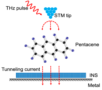
Figure 1: Light-assistend tunneling through a single molecule: schematic of a THz-STM experiment.

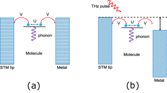
Figure 2: (a) Anderson-Holstein microscopic model for tunneling through a molecule. Only the HOMO orbital on the molecule is considered. Coulomb repulsion between electrons on the molecular orbital is included through the Anderson model. Interaction of electrons with the optical vibrational mode is included using the Holstein model. (b) Light assisted tunneling through a molecule in THz-STM experiments. Electric field from the femtosecond pulse modifies energy differences between the reservoirs and the molecular level.

In writing this paper we set ourselves two goals. Firstly, we present a new theoretical approach for analyzing non-equilibrium dynamics of the Anderson-Holstein impurity model. This method is based on the variational non-Gaussian wavefunctions introduced in Ref. Shi et al. (2018) and further extended in the context of quantum impurity models in Refs. Ashida et al. (2018a, b). This technique is versatile and can be applied to a broad class of nonequilibrium problems, including quenches, pump and probe experiments, and the analysis of AC and DC transport. Most of the previously developed approaches for the Anderson impurity problem focus either on high energy degrees of freedom on the scale of the electron-electron repulsion $U$ Ng and Lee (1988), or the low energy sector with the scale set by the Kondo temperature $T_{K}$ Wingreen and Meir (1993, 1994); Ng (1996); Kaminski et al. (2000). The advantage of our approach is that within the same framework it describes both high and low energy degrees of freedom without requiring numerical resources of NRG Hewson and Meyer (2002); Legeza et al. (2008); Holzner et al. (2010) or DMRG Al-Hassanieh et al. (2006); Heidrich-Meisner et al. (2009); Eckel et al. (2010). To establish the validity of the new method we verify that it correctly reproduces basic results of the canonical Anderson impurity model: it captures the Kondo resonance in the spectral function at the Fermi energy and gives a conductance $G=2e^{2}/h$ in the linear response regime. We extend the analysis of the Anderson model to include the electron-phonon interaction on the impurity site and demonstrate that coupling to the phonons can strongly suppress the Kondo peak. Our second goal in this paper is to analyze a specific type of nonequilibrium dynamics: THz STM experiments through a single molecule. For such experiments we compute the time dependence of the key observables: current through the system, number of electrons on the molecule, and number of excited phonons. To illustrate the important role of interactions in the system, we also discuss a non-interacting resonant level model (RLM)in the infinite bandwidth approximation. We show that, in this case, the transient current dynamics in the THz-STM experiemnts can be computed analytically. We discuss the difference in the results between the non-interacting RLM system and the Anderson-Holstein model.

I.2 Anderson-Holstein Model

The system we consider is shown schematically in Figs. 1 and 2. In the absence of laser light the chemical potential of the organic molecule is in the middle of the gap between the HOMO and LUMO orbitals of the molecule and there is no current through the system Cocker et al. (2016). The light pulse changes the relative energies of the molecular level and the reservoirs (see Fig. 2b) and allows for an ultrafast electron burst as a co-tunneling process between the STM tip, the molecule, and the metal. Due to the asymmetry of the electric field in the pulse Cocker et al. (2013); Yoshioka et al. (2016) it is sufficient to consider only one of the orbitals in the molecule, which we take to be the HOMO orbital. We model the interaction between HOMO electrons using the Anderson type local repulsion $U$ and include interaction of electrons with vibrations of the molecule Cocker et al. (2016) using Holstein type coupling of the phonon displacement to the number of electrons in the localized orbital Mahan (2000). Thus, molecular degrees of freedom are given by the Hamiltonian

$$\mathcal{H}_{\mathrm{mol}} = \mathcal{H}_{\mathrm{A}}+\mathcal{H}_{\mathrm{phon}},$$

$$\mathcal{H}_{\mathrm{A}} = \varepsilon_{d}n_{d}+Un_{\uparrow}n_{\downarrow},$$

$$\mathcal{H}_{\mathrm{phon}} = \omega_{b}b^{\dagger}b+g(2-n_{d})(b^{\dagger}+b).$$ (1)

Here, $d_{\sigma}$ are the annihilation operators of electrons in the HOMO, $n_{d}=n_{\uparrow}+n_{\downarrow}$ is the total number of electrons in the molecule $n_{\sigma=\uparrow\downarrow}=d_{\sigma}^{\dagger}d_{\sigma}$, $b$ is the annihilation operator for the phonon with frequency $\omega_{b}$, and $\varepsilon_{d}$ is the energy of the HOMO orbital.

We model the STM tip and the metallic electrode as one dimensional chains of non-interacting electrons because we do not expect appreciable dependence on the nature of electron reservoirs. Our analysis can be easily extended to other type of reservoirs.

$$\mathcal{H}_{\mathrm{a}=\mathrm{L,R}}=-t_{0}\sum_{\left\langle ij\right\rangle,\sigma}c_{i,\sigma,\mathrm{a}}^{\dagger}c_{j,\sigma,\mathrm{a}}-\mu_{\mathrm{a}}\sum_{j,\sigma}c_{j,\sigma,\mathrm{a}}^{\dagger}c_{j,\sigma,\mathrm{a}},$$ (2)

Here, $c_{j,\sigma,\mathrm{a}}$ denote annihilation operators of electrons with spin $\sigma$ in the reservoir $\mathrm{a}=\mathrm{L,R}$ at site $j$. Coupling between the molecule and reservoirs is included via the hybridization term

$$\mathcal{H}_{\mathrm{V}}=V\sum_{\sigma,\mathrm{a}}(c_{0,\sigma,\mathrm{a}}^{\dagger}d_{\sigma}+\mathrm{H.c.}).$$ (3)

Different chemical potentials of the reservoirs account for a finite time-dependent bias voltage, where we assume that all the time dependent potential is applied between the molecule and the right reservoir (our analysis can be easily generalized to the arbitrary time dependent potentials for both reservoirs)

$$V_{\mathrm{e}}(t)=\mu_{\mathrm{R}}(t)-\mu_{\mathrm{L}}.$$ (4)

The main effect of the femtosecond laser pulse is to change the bias voltage as shown in Fig. 2b.

The full Hamiltonian of the system is then given by

$$\mathcal{H}(t)=\mathcal{H}_{\mathrm{mol}}+H_{\mathrm{V}}+\sum_{a}\mathcal{H}_{\mathrm{a}}(t)$$ (5)

I.3 Review of the theoretical formalism

The theoretical modeling of light assisted tunneling of electrons through a single molecule requires the analysis of nonequilibrium dynamics of the Anderson impurity model with an added complication, that of the electron-phonon coupling. The Anderson impurity problem is one of the most fundamental models in the field of interacting electron systems. It provides the foundation for our understanding of a broad range of physical phenomena, including the Kondo effect in metals Mahan (2000); Hewson (1993), the electron transport in mesoscopic structures Kastner et al. (1998); S. M. Cronenwett et al. (1998); Kouwenhoven and Glazman (2001); Bolech and Shah (2016), the formation of heavy fermion electron systems Stewart (1979); Gegenwart et al. (2008); Si and Steglich (2010); Kotliar and Vollhardt (2004). A broad range of analytical tools has been developed to study equilibrium properties of this model including a Bethe ansatz solution Andrei et al. (1983); Wiegmann and Tsvelik (1984), the renormalization group approach Bulla et al. (2008), the slave-particle method Read and Newns (1983); Kroha and Wolfle (1999), and dynamical mean-field theory (DMFT) Georges et al. (1996); Feldbacher et al. (2004); Rubtsov et al. (2005); Werner et al. (2006); Gull et al. (2011). However, the non-equilibrium dynamics of the model remains poorly understood. While most of the theoretical work on quantum dynamics of the Anderson model relied on the non-crossing approximation Wingreen and Meir (1994); Anders and Grewe (1994), other promising new approaches utilized real-time DMFT Aoki et al. (2014) combining the bold-line quantum Monte Carlo technique with a memory function formalism Cohen et al. (2013). Calculations using either of these approaches are demanding in terms of numerical resources.

In this paper we propose a new approach to analyzing the Anderson-Holstein impurity model both in and out of equilibrium. This approach is based on combining a unitary transformation of the generalized-polaron type with a family of non-Gaussian variational states for quantum impurity problems. The electron-phonon part of the transformation entangles the electron and phonon degrees of freedom and allows us to use factorized wavefunctions, in which bosonic and electronic parts are described using a Gaussian ansatz and a family of non-Gaussian variational wavefunctions, respectively. The role of the unitary transformation in the non-Gaussian ansatz for the Anderson model is to utilize exact conservation laws to reduce the number of impurity degrees of freedom at the cost of introducing additional interactions and correlations between the bath particles. The key difference between our method and the traditional approaches based on the polaron transformations Mahan (2000) is that we allow parameters of the transformation to vary in time. The general philosophy of this method has been introduced earlier in Ref. Shi et al. (2018), which demonstrated that this technique successfully describes equilibrium and dynamical properties of many important solid state systems including polarons in the Su-Schrieffer-Heegger and Holstein models, spin-bath models, and superconductivity in the Holstein model. Recently, Ashida et al. Ashida et al. (2018a, b) demonstrated that this method efficiently captures the complicated dynamics of the anisotropic Kondo model, including the finite time crossover between the ferromagnetic and antoferromagnetic couplings Kanász-Nagy et al. (2018). Since this is the first time that this method is used to study the Anderson model, we include a separate analysis of the equilibrium properties including the electron spectral function. We demonstrate that our approach accurately captures the formation of the Kondo resonance at the Fermi energy with the width set by the Kondo energy scale. This demonstrates that our method is versatile and captures both short time/high energy and long time/low energy aspects of the Anderson model.

I.4 Organization of the paper

This paper is organized as follows: In Section II we introduce the general formalism of non-Gaussian variational wavefunctions. In Section III we use the imaginary time flow approach to analyze the ground state properties of the Anderson and Anderson-Holstein models focusing on the regimes of single and double occupancy of the localized orbital. We compute electron spectral functions and demonstrate that in the Kondo regime of the Anderson model our approach correctly reproduces a resonance at the Fermi level. We show how the spectral functions get modified upon adding the interaction with phonons. Two prominent features are the suppression of the Kondo resonance and the appearance of the phonon shake-off peaks. As additional check of the validity of our method we compute spin correlation functions between electrons on the localized orbital and in the electron reservoirs. We demonstrate that in the Kondo regime we get the expected oscillating correlations decaying as a power law of the distance to the localized orbital. In Section IV we introduce a real time analysis of the Anderson and Anderson-Holstein models. For the Anderson model we analyze the DC transport and compute the full non-linear conductance. We demonstrate that in the Kondo regime our method correctly gives a linear conductance equal to $2e^{2}/h$. For the Anderson-Holstein model, we focus on the analysis of photocurrent induced by the THz pulze in the single and double occupancy regimes. We present results for the time evolution of the current, the occupation number of the localized orbital, and the phonon displacement. We show the dependence of the total transferred charge on the amplitude of the electromagnetic pulse. Section V contains a summary of our results and a discussion of interesting open problems. Many technical details of the calculations are not presented in the main text of the paper but delegated to Appendices. This includes a derivation of the analytical results for photocurrent in the non-interacting resonant level model.

II Non-Gaussian variational ansatz

In this section, we introduce the variational ansatz

$$\left|\Psi_{\mathrm{NGS}}\right\rangle=U_{\mathrm{ph}}U_{\mathrm{A}}\left|\Psi_{\mathrm{GS}}\right\rangle_{f}\left|\Psi_{\mathrm{GS}}\right\rangle_{b},$$ (6)

which we will use to study both the ground state and non-equilibrium real-time dynamics. The unitary transformation $U_{\mathrm{ph}}$ entangles the phonon mode with the electronic degrees of freedom in HOMO and in the reservoirs. The unitary transformation $U_{\mathrm{A}}$ uses parity conservation to partially decouple the impurity degrees of freedom. Throughout the paper we use the terminology of the Anderson impurity model and refer to the electronic degrees of freedom in the molecule as impurity degrees of freedom. Finally $\left|\Psi_{\mathrm{GS}}\right\rangle_{f,b}$ are Gaussian states for electrons and the phonon mode.

II.1 Electron-phonon polaron transformation

The generalized polaron transformation $U_{\mathrm{ph}}=e^{S}$ is defined by the generating operator

$$S=iR^{T}\lambda(2-n_{d})$$ (7)

with the time-dependent variational parameters $\lambda=(\lambda_{x},\lambda_{p})^{T}$. Here $R=(x,p)=(b^{\dagger}+b,i(b^{\dagger}-b))^{T}$ is the quadrature of the phonon mode. When the polaron transformation (7) is applied to the system Hamiltonians

$$H_{1}=U_{\mathrm{ph}}^{\dagger}HU_{\mathrm{ph}}$$ (8)

we find that the lead Hamiltonians $\mathcal{H}_{\mathrm{L,R}}$ do not change, whereas the molecular part of the Hamiltonian $\mathcal{H}_{\mathrm{mol}}=\mathcal{H}_{\mathrm{A}}+\mathcal{H}_{\mathrm{phon}}$ becomes

$$\mathcal{H}_{\mathrm{A}} = \tilde{\varepsilon}_{d}n_{d}+\tilde{U}n_{\uparrow}n_{\downarrow}+4(\omega_{b}\lambda^{T}\lambda-2g\lambda_{p}),$$

$$\mathcal{H}_{\mathrm{phon}} = \frac{1}{4}\omega_{b}R^{T}R+(2-n_{d})R^{T}G_{\lambda},$$ (9)

and the hybridization term changes to

$$H_{\mathrm{V}}=Ve^{-iR^{T}\lambda}\sum_{\sigma,\mathrm{a}}c_{0,\sigma,\mathrm{a}}^{\dagger}d_{\sigma}+\mathrm{H.c.}.$$ (10)

The polaron transformation reduces the electron-phonon interaction to $G_{\lambda}=\left(g-\omega_{b}\lambda_{p},\omega_{b}\lambda_{x}\right)^{T}$, renormalizes the single particle energy level $\tilde{\varepsilon}_{d}=\varepsilon_{d}-3(\omega_{b}\lambda^{T}\lambda-2g\lambda_{p})$ and the on-site interaction $\tilde{U}=U+2(\omega_{b}\lambda^{T}\lambda-2g\lambda_{p})$, whereas the hybridization term $Ve^{-iR^{T}\lambda}$ between the phonon-dressed electrons in HOMO and reservoirs aquires polaronic dressing.

II.2 Parity operator and impurity decoupling transformation

Refs Shi et al. (2018); Ashida et al. (2018a) introduced an efficient way of solving quantum impurity problems by utilizing parity conservation. In particular, in the Kondo impurity problem one can construct an exact unitary transformation that maps the conserved parity operator to one of the components of the impurity spin. After the transformation, the impurity spin is decoupled from the reservoir at the cost of introducing interactions between bath fermions, which, however, can be effectively handled using the Gaussian part of the wavefunction. In this paper we generalize such transformation to the Anderson impurity problem. In the Anderson model one can not completely decouple the impurity from the reservoir, but it is possible to reduce the number of degrees of freedom so that the Gaussian ansatz for the wavefunction can be utilized efficiently.

To simplify notations we introduce a four component representation of the electronic Hilbert space on the molecule: $\{\left|0\right\rangle,\left|\uparrow\right\rangle=d_{\uparrow}^{\dagger}|0\rangle,\left|\downarrow\right\rangle=d_{\downarrow}^{\dagger}|0\rangle,\left|\uparrow\downarrow\right\rangle=d_{\uparrow}^{\dagger}d_{\downarrow}^{\dagger}|0\rangle\}$. We define four component matrices in this space so that the first Pauli matrix acts in the space (1,2) $\leftrightarrow$ (3,4). For example,

$$\sigma_{x}\otimes I=\left[\begin{array}[]{cc}\hat{0}&\hat{1}\\ \hat{1}&\hat{0}\end{array}\right]\hskip 28.45274pt\sigma_{z}\otimes I=\left[\begin{array}[]{cc}\hat{1}&\hat{0}\\ \hat{0}&\hat{-1}\end{array}\right]$$ (15)

When the Pauli matrix is in the second position in the tensor product, it acts simultaneously in sub-spaces 1 $\leftrightarrow$ 2, 3 $\leftrightarrow$ 4, so that

$$I\otimes\sigma_{x}=\left[\begin{array}[]{cc}\hat{\sigma_{x}}&\hat{0}\\ \hat{0}&\hat{\sigma_{x}}\end{array}\right]\hskip 28.45274ptI\otimes\sigma_{z}=\left[\begin{array}[]{cc}\hat{\sigma_{z}}&\hat{0}\\ \hat{0}&\hat{\sigma_{z}}\end{array}\right]$$ (20)

We define the parity operator for spin $\uparrow$ electrons on the molecule

$$\Sigma_{z}=e^{i\pi(d_{\uparrow}^{\dagger}d_{\uparrow}-1)}$$

The choice of the overall sign is a matter of convenience. In the tensor notations introduced earlier

$$\Sigma^{z}=-I\otimes\sigma^{z}$$

Note that the operator $\Sigma_{z}$ performs a $\pi$ rotation in the subspace ($|\uparrow\rangle$, $|\downarrow\rangle$) as well as a $\pi$ rotation in the subspace ($|0\rangle$, $|\uparrow\downarrow\rangle$). The parity operator for spin $\uparrow$ fermions in the bath is defined as

$$P_{z} = e^{i\pi N_{\uparrow}}$$ (21)

$$N_{\uparrow} = \sum_{j,\mathrm{a}}c_{j,\uparrow,\mathrm{a}}^{\dagger}c_{j,\uparrow,\mathrm{a}}$$ (22)

The parity operator for the system as a whole

$$P=\Sigma^{z}P_{z}$$

is conserved since the Hamiltonian preserves the number of electrons with a given spin. Mathematically this means that $[P,H_{1}]=0$.

In the spirit of RefsAshida et al. (2018a, b) we introduce a transformation that maps the conserved operator $P$ entirely into the impurity degrees of freedom. Following this transformation, the original conservation low for $P$ becomes a conservation law for the imourity electrons. We consider a unitary operator

$$U_{\mathrm{A}}=\frac{1}{\sqrt{2}}(1+i\Sigma^{y}P_{z})$$ (23)

with $\Sigma^{y}=-\sigma^{x}\otimes\sigma^{y}$ Direct calculation shows that

$$U_{\mathrm{A}}^{\dagger}PU_{\mathrm{A}}=\sigma^{x}\otimes\sigma^{x}\equiv X$$ (24)

We observe that the operator $X$ does not contain any degrees of freedom of the reservoir electrons. Another important feature of the operator $X$ is that it only connects states with the same electron parity, i.e. it does not mix between subspaces ($|\uparrow\rangle$, $|\downarrow\rangle$) and ($|0\rangle$, $|\uparrow\downarrow\rangle$). Hence the operator $X$ is bosonic and its eigenstates are physically well defined states. After performing the transformation $U_{\mathrm{A}}$ on the Hamiltonian

$$H_{2}=U_{\mathrm{A}}^{\dagger}H_{1}U_{\mathrm{A}}$$

we are guaranteed that the operator $X$ commutes with the transformed Hamiltonian $H_{2}$, which means that we reduced the number of degrees of freedom corresponding to the molecule. Let us discuss the implications of this fact in more detail. Operator $X$ has eigenvalues $\pm 1$. The eigenstates corresponding to the eigenvalue $+1$ make a two dimensional Hilbert space with basis vectors

$$|+_{s}\rangle = \frac{1}{\sqrt{2}}(|\uparrow\rangle+|\downarrow\rangle)$$

$$|+_{c}\rangle = \frac{1}{\sqrt{2}}(|0\rangle+|\uparrow\downarrow\rangle)$$ (25)

The eigenstates corresponding to the eigenvalue $-1$ make an orthogonal two dimensional Hilbert space with basis vectors

$$|-_{s}\rangle = \frac{1}{\sqrt{2}}(|\uparrow\rangle-|\downarrow\rangle)$$

$$|-_{c}\rangle = \frac{1}{\sqrt{2}}(|0\rangle-|\uparrow\downarrow\rangle)$$ (26)

Conservation of $X$ means that the dynamics described by the Hamiltonian $H_{2}$ can not mix between subspaces (25) and (26). Hence for the dynamics in the $+1$ subspace we need to consider only two electronic states in the molecule: $|+_{s}\rangle$ and $|+_{c}\rangle$. We introduce the fermion operator

$$f_{+}=(-)^{F}\,|+_{s}\rangle\langle+_{c}|$$

where $F=\sum_{j,\sigma,\mathrm{a}}c_{j,\sigma,\mathrm{a}}^{\dagger}c_{j,\sigma,\mathrm{a}}$ is the total number operator of electrons in both reservoirs. In the $+1$ subspace Hamiltonian $H_{2}$ can be expressed entirely in terms of the reservoir operators $c_{i,\sigma,a}$, for the molecule $f_{+}^{\pm}$, and phonon operators. Analogously, in the $-1$ subspace (26) we introduce the fermion operator that connects two states with different electron parity

$$f_{-}=(-)^{F}\,|-_{s}\rangle\langle-_{c}|$$

The explicit expression for $H_{2}$ can be obtained from a straightforward but somewhat lengthy calculation. The part of the Hamiltonian corresponding to the left and right reservoirs does not change. The part of $H_{2}$ corresponding to the molecule, $\mathcal{H}_{\mathrm{mol}}=\mathcal{H}_{\mathrm{A}}+\mathcal{H}_{\mathrm{phon}}$, becomes

$$H_{\mathrm{A}} = 4(\omega_{b}\lambda^{T}\lambda-2g\lambda_{p})+\tilde{\varepsilon}_{d}$$

$$+\frac{1}{2}\tilde{U}f_{\gamma}^{\dagger}f_{\gamma}+(\tilde{\varepsilon}_{d}+\frac{1}{2}\tilde{U})\gamma P_{z}f_{\gamma}^{\dagger}f_{\gamma},$$

$$H_{\mathrm{ph}} = \frac{1}{4}\omega_{b}R^{T}R+(1-\gamma P_{z}f_{\gamma}^{\dagger}f_{\gamma})R^{T}G_{\lambda},$$ (27)

The transformed hybridization term is given by

$$H_{\mathrm{V}} = \frac{V}{2}e^{-iR^{T}\lambda}\sum_{\mathrm{a}}[c_{0,\uparrow,\mathrm{a}}^{\dagger}(f_{\gamma}^{\dagger}+f_{\gamma})+\gamma c_{0,\downarrow,\mathrm{a}}^{\dagger}(f_{\gamma}^{\dagger}-f_{\gamma})$$ (28)

$$-P_{z}(\gamma c_{0,\uparrow,\mathrm{a}}^{\dagger}+c_{0,\downarrow,\mathrm{a}}^{\dagger})(f_{\gamma}^{\dagger}+f_{\gamma})]+\mathrm{H.c.},$$

II.3 Gaussian part of the wavefunction

A convenient way of defining Gaussian wavefunctions in equation (6) is to consider a unitary Gaussian transformation acting on the electron and phonon vacuum $\left|\Psi_{\mathrm{GS}}\right\rangle_{f}\left|\Psi_{\mathrm{GS}}\right\rangle_{b}=U_{\mathrm{GS}}\left|0\right\rangle$. The Gaussian state is completely characterized by the expectation values of the phonon quadratures $\Delta_{R}=\left\langle R\right\rangle$ and covariance matrices $\Gamma_{b}=\left\langle\{\delta R,\delta R^{T}\}\right\rangle_{\mathrm{GS}}/2$ and $\Gamma_{f}=\left\langle CC^{\dagger}\right\rangle_{\mathrm{GS}}$ for bosons and fermions respectively, where $\delta R=R-\Delta_{R}$ is the quadrature fluctuation around its mean value, and $C=(c,c^{\dagger})^{T}$ is defined in the Nambu space $c=(f,c_{j,\uparrow,\mathrm{L}},c_{j,\downarrow,\mathrm{L}},c_{j,\uparrow,\mathrm{R}},c_{j,\downarrow,\mathrm{R}})^{T}$. Alternatively, one can introduce the Majorana basis $A$ using $A=W_{f}C$ with

$$W_{f}=\left(\begin{array}[]{cc}{\openone}_{4N+1}&{\openone}_{4N+1}\\ -i{\openone}_{4N+1}&i{\openone}_{4N+1}\end{array}\right).$$ (29)

Majorana operators are given by linear combinations of the form $(c_{\alpha}+c_{\alpha}^{\dagger})$, $i(c_{\alpha}^{\dagger}-c_{\alpha})$. Then, the covariance matrix is defined as $\Gamma_{m}=i\left\langle[A,A^{\dagger}]\right\rangle_{\mathrm{GS}}/2$ Shi et al. (2018); Kraus and Cirac (2010).

In the next section we will obtain the variational ground state of the Anderson-Holstein model by analyzing the flow of variational parameters $\lambda$, $\Delta_{R}$, and $\Gamma_{b,f(m)}$ in imaginary time. We will then derive the real time equations of motion (EOM) which we will apply to study the dynamics.

III Ground state properties

In this section, we use imaginary time evolution to approximate the ground state of the Anderson-Holstein model. We will demonstrate that in the case of the canonical Anderson model our method correctly captures the non-perturbative Kondo effect, including the formation of a resonance at the Fermi energy and presence of characteristic spin correlations between the impurity and reservoir electrons indicating the presence of Kondo spin screening clouds. We project the equations of motion (EOM)

$$\partial_{\tau}\left|\Psi\right\rangle=-(H-\left\langle H\right\rangle)\left|\Psi\right\rangle$$ (30)

onto the tangential plane of the variational manifold (6), and obtain the EOM for the variational parameters $\lambda$, $\Delta_{R}$, and $\Gamma_{b,f(m)}$ (see Ref. Shi et al. (2018) for details). As $\tau\rightarrow\infty$ the system reaches a fixed point which approximates to the ground state of the system.

The steady state solution of the EOM in the limit $\tau\rightarrow\infty$ determines the ground state properties, including the occupation number, the magnetization, and the spectral function of electrons in HOMO, as well as correlation functions between HOMO and reservoirs.

III.1 Equations of motion in imaginary time

We first analyze the structure of the tangential vectors of the variational manifold (6). To this purpose, we introduce the unitary operator

$$U_{\mathrm{GS}}=e^{-\frac{1}{2}R^{T}\sigma^{y}\Delta_{R}}e^{-i\frac{1}{4}R^{T}\xi_{b}R}e^{i\frac{1}{2}C^{\dagger}\xi_{f}C}$$ (31)

that generates the Gaussian state and transforms $R$ and $C$ as $U_{\mathrm{GS}}^{\dagger}RU_{\mathrm{GS}}=SR+\Delta_{R}$ and $U_{\mathrm{GS}}^{\dagger}CU_{\mathrm{GS}}=U_{f}C$. The covariance matrices $\Gamma_{b}=SS^{T}$ and $\Gamma_{f}=U_{f}(1+\sigma^{z})U_{f}^{\dagger}/2$ are related to the symplectic and unitary transformations via $S=e^{i\sigma^{y}\xi_{b}}$ and $U_{f}=e^{i\xi_{f}}$.

Let us consider the tangential vector for the variational wavefunction (6). It is defined as the derivative of $\left|\Psi_{\mathrm{NGS}}\right\rangle$ with respect to $\tau$

$$\partial_{\tau}\left|\Psi_{\mathrm{NGS}}\right\rangle=U_{\mathrm{ph}}U_{\mathrm{A}}U_{\mathrm{GS}}(V_{1}+V_{2}+V_{h})\left|0\right\rangle,$$ (32)

We separated the $V_{1}$, $V_{2}$, $V_{h}$ terms in equation (32) based on the number of creation and annihilation operators.

The $V_{1}$ term in (32) is linear in phonon operators

$$V_{1}=R^{T}S^{T}[i(1-\gamma\left\langle P_{z}f_{\gamma}^{\dagger}f_{\gamma}\right\rangle_{\mathrm{GS}})\partial_{\tau}\lambda-\frac{1}{2}\sigma^{y}\partial_{\tau}\Delta_{R}]$$ (33)

It is determined by the expectation value $\left\langle P_{z}f_{\gamma}^{\dagger}f_{\gamma}\right\rangle_{\mathrm{GS}}$ in the Gaussian state.

The $V_{2}$ term in (32) is quadratic in phonon and electron creation/annihilation operators

$$V_{2}=-\frac{1}{4}\text{:}R^{T}S^{T}\sigma^{y}\partial_{\tau}SR\text{:}+\frac{1}{2}\text{:}C^{\dagger}U_{f}^{\dagger}(\partial_{\tau}+O_{f})U_{f}C\text{:}$$ (34)

Note that since the operator $V_{2}$ acts on the vacuum state we should bring it to normal ordered form. This is indicated by “::” in equation (34). Due to the presence of matrices performing rotations of creation/annihilation operators, $S$ for phonons and $U_{f}$ for fermions, this normal ordering is with respect to the instantaneous Gaussian state. The matrix $O_{f}$ is defined from

$$O_{f}=-\lambda^{T}\sigma^{y}\partial_{\tau}\lambda\sigma^{z}\otimes I_{f}+\gamma(2\lambda^{T}\sigma^{y}-i\Delta_{R}^{T})\partial_{\tau}\lambda O_{P}$$ (35)

where the diagonal matrix $I_{f}$ has only one non-zero element $(I_{f})_{11}=1$, and

$$O_{P}=2iW_{f}^{\dagger}\frac{\delta}{\delta\Gamma_{m}}\left\langle P_{z}f_{\gamma}^{\dagger}f_{\gamma}\right\rangle_{\mathrm{GS}}W_{f};$$ (36)

The $V_{h}$ term in equation (32)

$$V_{h} = \gamma[(2\lambda^{T}\sigma^{y}-i\Delta_{R}^{T})U_{\mathrm{GS}}^{\dagger}P_{h}U_{\mathrm{GS}}$$ (37)

$$-iR^{T}S^{T}U_{\mathrm{GS}}^{\dagger}P_{c}U_{\mathrm{GS}}]\partial_{\tau}\lambda$$

contains higher order terms defined by the expansion

$$P_{z}f_{\gamma}^{\dagger}f_{\gamma} = \left\langle P_{z}f_{\gamma}^{\dagger}f_{\gamma}\right\rangle_{\mathrm{GS}}+P_{c},$$

$$P_{c} = \frac{1}{2}\text{:}C^{\dagger}O_{P}C\text{:}+P_{h}$$ (38)

Equation (38) should be understood as the definition of $P_{h}$.

The projection on the tangential vector $U_{\mathrm{ph}}U_{\mathrm{A}}U_{\mathrm{GS}}V_{1}\left|0\right\rangle$ leads to EOM for the expectation value of the phonon quadrature $\Delta_{R}$

$$\partial_{\tau}\Delta_{R} = -\Gamma_{b}[\omega_{b}\Delta_{R}-2\lambda\text{Im}\left\langle\mathcal{I}_{dc}\right\rangle_{\mathrm{GS}}$$ (39)

$$+2(1-\gamma\left\langle P_{z}f_{\gamma}^{\dagger}f_{\gamma}\right\rangle_{\mathrm{GS}})G_{\lambda}]$$

$$+2i(1-\gamma\left\langle P_{z}f_{\gamma}^{\dagger}f_{\gamma}\right\rangle_{\mathrm{GS}})\sigma^{y}\partial_{\tau}\lambda$$

where

$$\mathcal{I}_{dc} = Ve_{\lambda}\sum_{\mathrm{a}}[P_{z}(f_{\gamma}^{\dagger}+f_{\gamma})(\gamma c_{0,\uparrow,\mathrm{a}}-c_{0,\downarrow,\mathrm{a}})$$ (40)

$$+(f_{\gamma}^{\dagger}+f_{\gamma})c_{0,\uparrow,\mathrm{a}}-\gamma(f_{\gamma}^{\dagger}-f_{\gamma})c_{0,\downarrow,\mathrm{a}}],$$

and the effective hybridization strength $V_{\mathrm{eff}}=Ve_{\lambda}$ is reduced by the factor $e_{\lambda}\equiv\left\langle e^{iR^{T}\lambda}\right\rangle_{\mathrm{GS}}=e^{i\Delta_{R}^{T}\lambda}e^{-\frac{1}{2}\lambda^{T}\Gamma_{b}\lambda}$.

The projection on the tangential vector $U_{\mathrm{ph}}U_{\mathrm{A}}U_{\mathrm{GS}}V_{2}\left|0\right\rangle$ results in EOM

$$\partial_{\tau}\Gamma_{b} = \sigma^{y}\Omega_{\mathrm{re}}\sigma^{y}-\Gamma_{b}\Omega_{\mathrm{re}}\Gamma_{b},$$ (41)

$$\partial_{\tau}\Gamma_{m} = -\mathcal{H}_{m}-\Gamma_{m}\mathcal{H}_{m}\Gamma_{m}+i[\Gamma_{m},O_{m}]$$ (42)

for the covariance matrices $\Gamma_{b,m}$, where $\Omega_{\mathrm{re}}=\omega_{b}I_{2}-2$Re$\left\langle\mathcal{I}_{dc}\right\rangle_{\mathrm{GS}}\lambda\lambda^{T}$ and $\mathcal{H}_{m}$ are the mean-field single particle Hamiltonians of phonon and electrons, and $O_{m}=-iW_{f}O_{f}W_{f}^{\dagger}/2$. The explicit form of $\mathcal{H}_{m}$ is shown in Appendix A.

By projecting on the tangential vector $U_{\mathrm{ph}}U_{\mathrm{A}}U_{\mathrm{GS}}V_{h}\left|0\right\rangle$, we obtain EOM

$$\partial_{\tau}\lambda^{T}\mathbf{G}\partial_{\tau}\lambda=\partial_{\tau}\lambda^{T}\xi_{\tau}.$$ (43)

The explicit form of the Gram matrix $\mathbf{G}$ and the vector $\xi_{\tau}$ is given in Appendix A. By solving Eqs. (39), (41), (42) and (43) numerically, we obtain the ground state configuration in the limit $\tau\rightarrow\infty$. We note that the EOM (43) is quadratic in $\partial_{\tau}\lambda$, but it can be reduced to the linear ordinary differential equation (ODE) (see Appendix B).

III.2 Physical observables

In this subsection we will discuss several physical quantities that can be used to characterize the ground state of the Anderson-Holstein model (here the bias voltage $V_{e}=0$).

In the sector $\gamma$, the ground state energy $E_{\gamma}=E_{\mathrm{res}}+E_{\mathrm{mol}}+E_{V}$ is composed of a reservoir part $E_{\mathrm{res}}=\sum_{ij,\sigma,\mathrm{a}}h_{\mathrm{a},ij}\left\langle c_{i,\sigma,\mathrm{a}}^{\dagger}c_{j,\sigma,\mathrm{a}}\right\rangle_{\mathrm{GS}}$, the molecular energy $E_{\mathrm{mol}}=E_{\mathrm{A}}+E_{\mathrm{phon}}$:

$$E_{\mathrm{A}} = \tilde{\varepsilon}_{d}+\frac{1}{2}\tilde{U}\left\langle f_{\gamma}^{\dagger}f_{\gamma}\right\rangle_{\mathrm{GS}}+\frac{1}{2}U_{P}\gamma\left\langle P_{z}f_{\gamma}^{\dagger}f_{\gamma}\right\rangle_{\mathrm{GS}},$$

$$E_{\mathrm{phon}} = \frac{1}{4}\omega_{b}(\Delta_{R}^{T}\Delta_{R}+tr\Gamma_{b})-\frac{1}{2}\omega_{b}+\Delta_{R}^{T}G_{\lambda}$$ (44)

$$+4(\omega_{b}\lambda^{T}\lambda-2g\lambda_{p}),$$

and the hybridization energy $E_{V}=$Re$\left\langle\mathcal{I}_{dc}\right\rangle_{\mathrm{GS}}$, where $h_{\mathrm{a}=\mathrm{L,R}}=I_{2}\otimes(-t_{0}\delta_{i,j\pm 1}-\mu_{\mathrm{a}}\delta_{ij})$. As pointed out in Ref Shi et al. (2018) the energy $E_{\gamma}$ monotonically decreases during the imaginary time evolution.

The occupation number and the magnetization of electrons in HOMO are given by $\left\langle n_{d}\right\rangle=1+\gamma\left\langle P_{z}f_{\gamma}^{\dagger}f_{\gamma}\right\rangle_{\mathrm{GS}}$ and $m_{z}=\gamma\left\langle P_{z}(1-f_{\gamma}^{\dagger}f_{\gamma})\right\rangle_{\mathrm{GS}}$, respectively. Correlation between electrons in the HOMO and reservoirs are characterized by the correlation functions $C_{\alpha=x,y,z}=\left\langle d^{\dagger}\tau^{\alpha}dc_{j}^{\dagger}\tau^{\alpha}c_{j}\right\rangle/4$, where $\tau^{\alpha}$ is the Pauli matrix. In the transformed frame, the correlation functions can be expressed as expectation values computed in the Gaussian state

$$C_{x} = \frac{1}{4}\gamma\left\langle(1-f_{\gamma}^{\dagger}f_{\gamma})c_{j}^{\dagger}\tau^{x}c_{j}\right\rangle_{\mathrm{GS}},$$

$$C_{y} = -i\frac{1}{4}\left\langle P_{z}(1-f_{\gamma}^{\dagger}f_{\gamma})c_{j}^{\dagger}\tau^{y}c_{j}\right\rangle_{\mathrm{GS}},$$

$$C_{z} = \frac{1}{4}\gamma\left\langle P_{z}(1-f_{\gamma}^{\dagger}f_{\gamma})c_{j}^{\dagger}\tau^{z}c_{j}\right\rangle_{\mathrm{GS}}$$ (45)

The hole excitations in HOMO interact with the charge in the substrate via the Coulomb interaction, which results in the displacement

$$\left\langle R\right\rangle=\Delta_{R}-2i\sigma^{y}\lambda(1-\gamma\left\langle P_{z}f_{\gamma}^{\dagger}f_{\gamma}\right\rangle_{\mathrm{GS}})$$ (46)

of phonon.

The spectral function $\mathcal{A}(\omega)=-$Im$G_{R}(\omega)/\pi$ characterizes the properties of excitations above the ground state. More specifically, for the Anderson-Holstein system, it is determined by the Fourier transform $G_{R}(\omega)=\int dte^{i\omega t}G_{R}(t)$ of the retarded Green function

$$G_{R}(t)=-i\left\langle\{d_{\downarrow}(t),d_{\downarrow}^{\dagger}(0)\}\right\rangle\theta(t).$$ (47)

Following the unitary transformation given by $U_{\mathrm{ph}}U_{\mathrm{A}}$, the Green’s function becomes

$$G_{R}(t)=-i\left\langle\{\bar{d}_{\downarrow}(t),\bar{d}_{\downarrow}^{\dagger}(0)\}\right\rangle_{\mathrm{GS}}\theta(t),$$ (48)

where the evolution $\bar{d}_{\downarrow}(t)=e^{iH_{2}t}\bar{d}_{\downarrow}e^{-iH_{2}t}$ of the fermionic operator $\bar{d}_{\downarrow}=e^{-iR^{T}\lambda}F$ is governed by the Hamiltonian $H_{2}$, and

$$F=\frac{1}{2}[\gamma(f_{\gamma}^{\dagger}-f_{\gamma})-P_{z}(f_{\gamma}^{\dagger}+f_{\gamma})].$$ (49)

We approximate $\bar{d}_{\downarrow}(t)\sim e^{iH_{\mathrm{MF}}t}\bar{d}_{\downarrow}e^{-iH_{\mathrm{MF}}t}$ by the mean-field Hamiltonian $H_{\mathrm{MF}}=H_{\mathrm{MF}}^{p}+H_{\mathrm{MF}}^{e}$ with $H_{\mathrm{MF}}^{p}=\delta R^{T}\Omega_{\mathrm{re}}\delta R/4$ and $H_{\mathrm{MF}}^{e}=iA^{T}\mathcal{H}_{m}A/4$, where $\Omega_{\mathrm{re}}$ and $\mathcal{H}_{m}$ are determined by the average value of quadrature and covariance matrices in the ground state. Since the bosonic and electronic parts in the Gaussian state are factorized, the retarded Green function reads

$$G_{R}(t) = -i\theta(t)[\left\langle e^{-iR^{T}(t)\lambda}e^{iR^{T}\lambda}\right\rangle_{\mathrm{GS}}\left\langle F(t)F^{\dagger}\right\rangle_{\mathrm{GS}}$$ (50)

$$+\left\langle e^{iR^{T}\lambda}e^{-iR^{T}(t)\lambda}\right\rangle_{\mathrm{GS}}\left\langle F^{\dagger}F(t)\right\rangle_{\mathrm{GS}}].$$

The Green function $G_{R}(t)$ contains the average values on the Gaussian state, which can be obtained analytically in terms of the covariance matrices and $\Delta_{R}$ (see Appendix C). For instance,

$$\left\langle e^{-iR^{T}(t)\lambda}e^{iR^{T}\lambda}\right\rangle_{\mathrm{GS}} = e^{-\alpha}\sum_{n=0}^{\infty}\frac{\alpha^{n}}{n!}e^{-in\omega_{\mathrm{re}}t},$$

$$\left\langle e^{iR^{T}\lambda}e^{-iR^{T}(t)\lambda}\right\rangle_{\mathrm{GS}} = e^{-\alpha}\sum_{n=0}^{\infty}\frac{\alpha^{n}}{n!}e^{in\omega_{\mathrm{re}}t}.$$ (51)

where $\alpha=\lambda^{T}\Gamma_{b}\lambda$ and $\omega_{\mathrm{re}}$ is the simplectic eigenvalue of $\Omega_{\mathrm{re}}$.

Eventually, the imaginary part of the Fourier transform

$$G^{>}(\omega) = -i\int_{0}^{\infty}dte^{i(\omega+i\delta)t}\left\langle F(t)F^{\dagger}\right\rangle_{\mathrm{GS}},$$

$$G^{<}(\omega) = -i\int_{0}^{\infty}dte^{i(\omega+i\delta)t}\left\langle F^{\dagger}F(t)\right\rangle_{\mathrm{GS}}$$ (52)

gives the spectral function

$$\mathcal{A}(\omega) = -\frac{1}{\pi}e^{-\alpha}\sum_{n=0}^{\infty}\frac{\alpha^{n}}{n!}\text{Im}[G^{>}(\omega-n\omega_{\mathrm{re}})$$ (53)

$$+G^{<}(\omega+n\omega_{\mathrm{re}})],$$

where we add a small imaginary part $i\delta$ in the numerical calculation of Fourier transforms $G^{>(<)}$.

In the next two subsections, we show the occupation number, the correlation functions, the displacement, and the spectral function for the Anderson-Holstein model.

III.3 Anderson model in equilibrium

In this subsection, we present results for the ground state properties of the Anderson model, i.e. when the electron-phonon coupling $g=0$. We expect that in the Kondo regime $\varepsilon_{d}<0$, $\varepsilon_{d}+U>0$, and $\Gamma=V^{2}<(U,\varepsilon_{d})$, HOMO is singly occupied, i.e., $\left\langle n_{d}\right\rangle\sim 1$ and its magnetization $m_{z}=0$, which reflects screening of the impurity spin by electrons in reservoirs. An important signature of the Kondo regime of the Anderson model is the formation of anti-ferromagnetic correlations between spins of electrons in HOMO and on the adjacent sites in the reservoirs. These correlations will be absent when the impurity is in the doubly occupied regime with $\varepsilon_{d}<\varepsilon_{d}+U<0$ and $\left\langle n_{d}\right\rangle\sim 2$, which is relevant to the HOMO in the THz STM experiments.

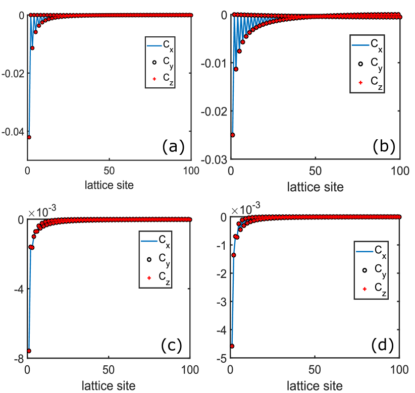
Figure 3: The correlation functions $C_{\alpha}$ in the Kondo regime (a)-(b) and the double occupation regime (c)-(d), where $\varepsilon_{d}=-0.5$ the hopping amplitude $t_{0}$ is taken as the unit. (a) $U=1$ and $\Gamma=0.16$; (b) $U=1$ and $\Gamma=0.04$; (c) $U=0.25$ and $\Gamma=0.04$; (c) $U=0.05$ and $\Gamma=0.04$.

In Fig. 3, we plot the correlation functions $C_{\alpha=x,y,z}$ of the electrons in HOMO and one of the reservoirs in the Kondo regime $(U,\varepsilon_{d},\Gamma)=(1,-0.5,0.16)$ and $(1,-0.5,0.04)$, and the double occupation regime $(0.25,-0.5,0.04)$ and $(0.05,-0.5,0.04)$. In the Kondo regime (Figs. 3a and 3b), the $SU(2)$-symmetric $C_{\alpha}$ shows significant anti-ferromagnetic correlations of electrons in the HOMO and the reservoirs. In the double occupation regime (Figs. 3c and 3d) we observe small values of the correlations $C_{\alpha}\sim 10^{-3}$, which indicates weak correlations between the singlet electron pair in the HOMO and the reservoirs.

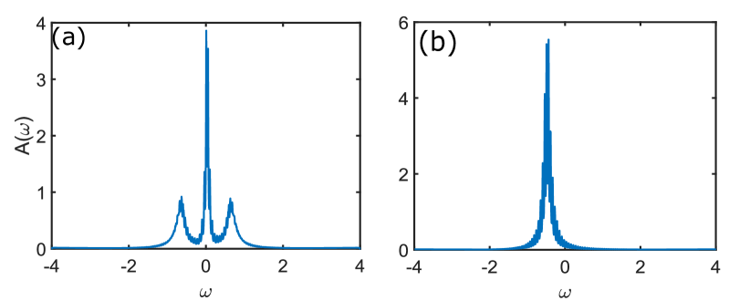
Figure 4: Electron spectral function in the localized orbital in the Kondo and double occupancy regimes without the electron-phonon interaction. System size is 100 and the hopping amplitude $t_{0}$ is taken as the unit: (a) $(U,\varepsilon_{d},\Gamma)=(1,-0.5,0.04)$ in the Kondo regime; (b) $(U,\varepsilon_{d},\Gamma)=(0.05,-0.5,0.04)$ in the double occupancy regime.

In Fig. 4, we show the spectral function $\mathcal{A}(\omega)$ in the Kondo and the doubly occupied regimes, where we take $\delta=0.01$. In Fig. 4a, the spectral function in the Kondo regime $(U,\varepsilon_{d},\Gamma)=(1,-0.5,0.04)$ displays both the Kondo resonance peak around $\omega=0$ and the resonance with energy levels $\varepsilon_{d}$ and $\varepsilon_{d}+U$. In the the double occupation regime $(U,\varepsilon_{d},\Gamma)=(0.05,-0.5,0.04)$, as shown in Fig. 4b, the Kondo resonance peak vanishes.

III.4 Anderson-Holstein model

In this subsection, we present results for the equilibrium properties of the full Anderson-Holstein model with finite electron-phonon interaction. Consequencies of the electron-phonon interaction $g$ include a change of the effective single particle energy level, softening of the on-site repulsive interaction, and polaronic dressing of hybridization. Note, for example, that when the occupation number on the molecular orbital $n_{d}$ is different from two, we get a finite displacement of the phonon operator $x_{0}=\left\langle x\right\rangle$, which favors partial occupation of the HOMO. We observe that in the Kondo regime including the electron-phonon intraction tends to suppress the formation of the singlet cloud, while in the doubly occupied regime it favors the creation of the hole excitations in HOMO.

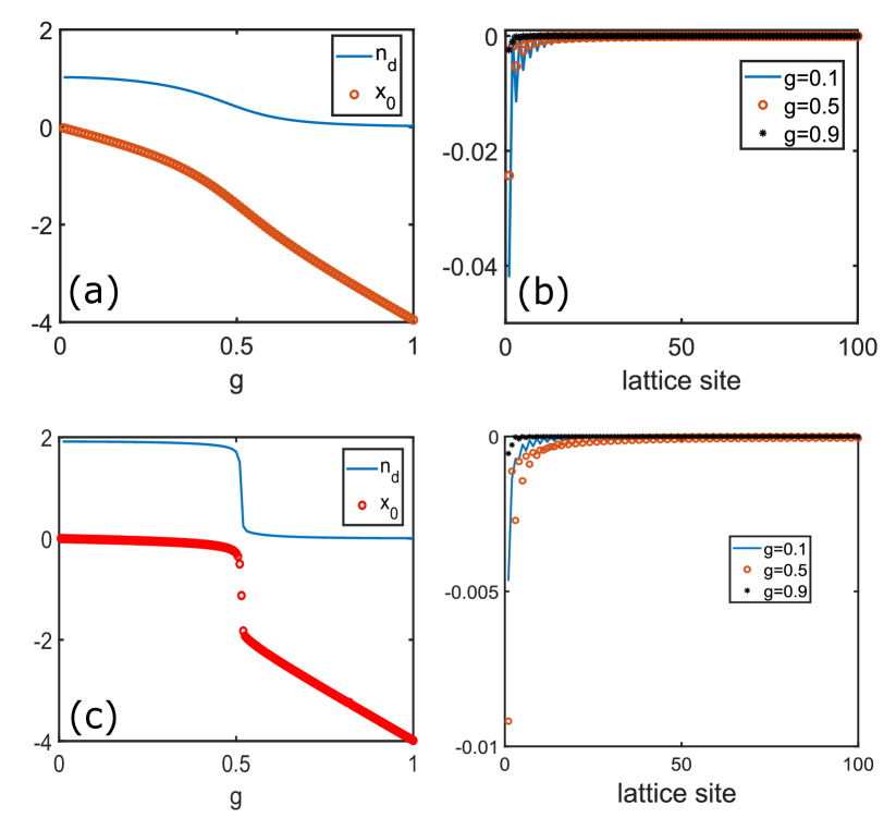
Figure 5: The occupation number $n_{d}$, the displacement $x_{0}$, and the correlation function $C_{\alpha}$ in the Kondo regime (a)-(b) and the double occupation regime (c)-(d), where $\varepsilon_{d}=-0.5$, $\omega_{b}=1$, and the hopping amplitude $t_{0}$ is taken as the unit. (a) The occupation number $n_{d}$ and the displacement $x_{0}$ for $U=1$ and $\Gamma=0.16$; (b) The correlation function $C_{\alpha}$ for $U=1$ and $\Gamma=0.16$; (c) The occupation number $n_{d}$ and the displacement $x_{0}$ for $U=0.05$ and $\Gamma=0.04$; (d) The correlation function $C_{\alpha}$ for $U=0.05$ and $\Gamma=0.04$.

In Fig. 5a, we show the occupation number $n_{d}$ and the displacement $x_{0}$ as a function of the coupling strength $g$ in the Kondo regime $(U,\varepsilon_{d},\Gamma)=(1,-0.5,0.16)$, where the magnetization $m_{z}=0$. In Fig. 5b, we show the correlation function $C_{\alpha}$ for different $g=0.1$, $0.5$, and $0.9$ in the Kondo regime. As $g$ increases, the displacement $x_{0}$ becomes larger, which lifts the single particle energy level of HOMO, therefore the the occupation number $n_{d}$ decreases from $1$ to $0$. The finite electron-phonon interaction also softens the on-site interaction and the effective hybridization strength $V_{\mathrm{eff}}<V$, thus, as shown in Fig. 5b, the larger the coupling strength $g$, the weaker the correlation $C_{\alpha}$ between HOMO and leads. Eventually, the Kondo singlet is destroyed by the finite electron-phonon coupling.

In Fig. 5c, we show the occupation number $n_{d}$ and the displacement $x_{0}$ as a function of $g$ in the double occupation regime $(U,\varepsilon_{d},\Gamma)=(0.05,-0.5,0.04)$, where the magnetization $m_{z}=0$. In Fig. 5d, we show the correlation functions $C_{\alpha}$ for different $g=0.1$, $0.5$, and $0.9$ in the double occupation regime. Since the single particle energy level is lifted, the particle number $n_{d}$ decreases from $2$ to $0$ as $g$ increases. For small electron-phonon couplings, e.g., $g=0.1$, HOMO is mostly doubly occupied, and $C_{\alpha}$ displays a weak correlation of HOMO and reservoirs. In the intermediate coupling regime, e.g., $g=0.5$, the occupation number $n_{d}$ decreases to $1.5$, meaning that electrons in HOMO are in the superposition of doubly and singly occupied states. Since the total spin in HOMO is totally screened, i.e., $m_{z}=0$, the singly occupied electron forms the singlet state with lead electrons. This explains somewhat the presence of a stronger correlation $C_{\alpha}$ in the intermediate regime than that in the weakly coupling regime. When $g$ increases further, e.g. to $g=0.9$, the occupation number $n_{d}$ is reduced to $0$, and the correlation $C_{\alpha}$ becomes vanishingly small.

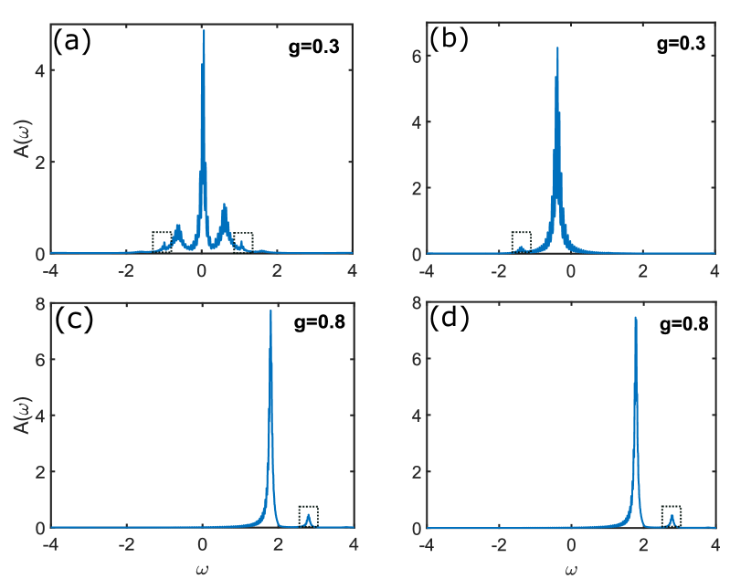
Figure 6: Electron spectral function in the localized orbital in the Kondo and double occupancy regimes including electron-phonon interaction. System size is 100 and the hopping amplitude $t_{0}$ is taken as the unit: (a) and (c) $(U,\varepsilon_{d},\Gamma)=(1,-0.5,0.04)$ in the Kondo regime; (b) and (d) $(U,\varepsilon_{d},\Gamma)=(0.05,-0.5,0.04)$ in the double occupancy regime.

In Fig. 6, we show the spectral function $\mathcal{A}(\omega)$ in the Kondo and doubly occupied regimes. In Fig. 6a, the spectral function $\mathcal{A}(\omega)$ in the Kondo regime $(U,\varepsilon_{d},\Gamma)=(1,-0.5,0.04)$ is shown, where the coupling strength $g=0.2$ and $0.4$. For $g=0.2$, the renormalized single particle energy level is slightly lifted to $\tilde{\varepsilon}_{d}\sim-0.40$ and the on-site interaction $\tilde{U}\sim 0.93$ is softened due to the electron-phonon interaction. Since $\tilde{\varepsilon}_{d}<0$ and $\tilde{\varepsilon}_{d}+\tilde{U}>0$ still in the Kondo regime, the Kondo peak survives in the spectral function. However, the system deviates from the symmetric Anderson model, i.e., $\left|\tilde{\varepsilon}_{d}\right|\neq\tilde{\varepsilon}_{d}+\tilde{U}$, therefore, in the spectral function, the two peaks around $\tilde{\varepsilon}_{d}$ and $\tilde{\varepsilon}_{d}+\tilde{U}$ become asymmetric. The small $\alpha\sim 0.02$ shows that the electron excitation in HOMO is weakly dressed by the phonon, and the spectral function is dominated by the pure electron excitation with the phonon in the vacuum state, i.e., $n=0$ in Eq. (53). For the larger $g=0.4$, $\tilde{\varepsilon}_{d}$ is shifted to $-0.06$ and the on-site interaction is reduced to $\tilde{U}\sim 0.71$. The spectral function shows that the Kondo peak is destroyed, and two peaks around $\tilde{\varepsilon}_{d}$ and $\tilde{\varepsilon}_{d}+\tilde{U}$ still survive. Since the electron excitation in HOMO is dressed by the phonon with larger average phonon number $\alpha\sim 0.08$, two peaks corresponding to the single phonon excitation appear in the spectral function, as shown in the (black) box of Fig. 6a.

In Fig. 6b we show the spectral function $\mathcal{A}(\omega)$ in the doubly occupied regime $(U,\varepsilon_{d},\Gamma)=(0.05,-0.5,0.04)$ for two values of the electron-phonon coupling strength $g=0.2$ and $0.4$. We point out that for $g=0.2$ the renormalized single particle energy level is shifted to $\tilde{\varepsilon}_{d}\sim-0.41$ and the on-site electron-electron interaction becomes effectively attractive $\tilde{U}\sim-0.01$ due to the phonon mediated attraction. The small $\alpha\sim 0.01$ implies that the electron in HOMO is weakly dressed by the phonon mode, as a result, the contribution of the phonon excitation to the spectral function is negligible. Comparing with the spectral function without electron-phonon interaction, we find that the peak is shifted to the larger frequency around the lifted single particle level $\tilde{\varepsilon}_{d}$. When the coupling constant is further increasing, e.g., $g=0.4$, $\tilde{\varepsilon}_{d}$ is shifted to $-0.1$ and the attractive interaction $\tilde{U}\sim-0.22$ becomes stronger. The electron excitation in HOMO is dressed by phonons with larger average number $\alpha\sim 0.06$, which results in the visible peak corresponding to the single phonon exitation, as shown in the (black) box of Fig. 6b.

IV Real time dynamics

In this section, we apply the non-Gaussian ansatz (6) to study real-time dynamics for the Anderson-Holstein system. Similar to the procedure used in the imaginary time evolution, we project the Schrödinger equation

$$i\partial_{t}\left|\Psi\right\rangle=H\left|\Psi\right\rangle$$ (54)

to the tangential space of the variational manifold (6) and obtain EOM for variational parameters $\lambda$, $\Delta_{R}$, and $\Gamma_{b,f(m)}$. Analysis of these differential equations allows us to explore a large variety of non-equilibrium phenomena

We now present results for transport through the molecule in the two cases: with and without electron-phonon interaction. To find DC conductance we perform a quench-type protocol, when we start with the reservoirs at different chemical potentials but disconnected from the molecule, and hence from each other. We switch on the molecule-reservoirs coupling and then evolve the system in real time until it reaches the steady state but before electron wavepackets reflected from the outer ends arrive back at the molecule. The steady state current $I$ as a function of (finite) $V_{e}$ gives us the full nonlinear current voltage characteristic of the system. Differential conductance is defined through the relation $\sigma_{c}=\partial_{V_{e}}I$. In the case of ultrafast THz STM experiments, bias voltage is applied as a time dependent pulse given in equation (62). This voltage pulse results in a transfer of a finite number of electrons between the two reservoirs. We compute the full time dependent evolution of the current in the system. We demonstrate that in the case of finite electron-phonon interaction a burst of current gives rise to vibrations of the molecules which persist well after the duration of the pulse. This was observed in experiments by Cocker et al. Cocker et al. (2016).

IV.1 Equations of motion

Projection of Eq. (54) to the tangential vectors $U_{\mathrm{ph}}U_{\mathrm{A}}U_{\mathrm{GS}}V_{1,2,h}\left|0\right\rangle$ gives EOM for variational parameters in the real time evolution. When we perform projection on the vectors $U_{\mathrm{ph}}U_{\mathrm{A}}U_{\mathrm{GS}}V_{1,2}\left|0\right\rangle$ we find in

$$\partial_{t}\Delta_{R} = i\sigma^{y}[\omega_{b}\Delta_{R}-2\lambda\text{Im}\left\langle\mathcal{I}_{dc}\right\rangle_{\mathrm{GS}}$$ (55)

$$+2(1-\gamma\left\langle P_{z}f_{\gamma}^{\dagger}f_{\gamma}\right\rangle_{\mathrm{GS}})G_{\lambda}$$

$$+2(1-\gamma\left\langle P_{z}f_{\gamma}^{\dagger}f_{\gamma}\right\rangle_{\mathrm{GS}})\partial_{t}\lambda],$$

$$\partial_{t}\Gamma_{b}=i(\sigma^{y}\Omega_{\mathrm{re}}\Gamma_{b}-\Gamma_{b}\Omega_{\mathrm{re}}\sigma^{y}),$$ (56)

and

$$\partial_{t}\Gamma_{m}=[\mathcal{H}_{m}-iO_{m},\Gamma_{m}].$$ (57)

To obtain the time evolution of $\lambda$, we perform the projection on the tangential vector $U_{\mathrm{ph}}U_{\mathrm{A}}U_{\mathrm{GS}}V_{h}\left|0\right\rangle$ and obtain

$$\partial_{t}\lambda^{T}\mathbf{M}\partial_{t}\lambda=\partial_{t}\lambda^{T}\xi_{t}$$ (58)

where $\xi_{t}=i\xi_{\tau}$. While Eq. (58) is non-linear in $\lambda$, it can be reduced to a linear ODE. Details are presented in Appendix B.

Thus, the description of a broad range of non-equilibrium phenomena in the Anderson-Holstein model can be reduced to solving Eqs. (55)-(58) for the time evolution of variational parameters.

Before presenting results of our analysis we comment on one important technical aspect of the calculations. The total electron number operators

$$N_{\uparrow} = \frac{1}{2}(1+\gamma P_{z})+\sum_{i,\mathrm{a}}c_{i,\uparrow,\mathrm{a}}^{\dagger}c_{i,\uparrow,\mathrm{a}},$$

$$N_{\downarrow} = \frac{1}{2}(1-\gamma P_{z})+\gamma P_{z}f_{\gamma}^{\dagger}f_{\gamma}+\sum_{i,\mathrm{a}}c_{i,\downarrow,\mathrm{a}}^{\dagger}c_{i,\downarrow,\mathrm{a}}$$ (59)

should be conserved throughout the real time evolution. This fundamental conservation law should not be affected by the transformations of the Hamiltonian $U_{ph}$ and $U_{A}$. However, when computing long time evolution needed for finding steady states the numerical errors may accumulate and lead to the violation of particle number conservation. To circumvent this numerical problem, we introduce a penalty term

$$H_{\Lambda}=\Lambda[(N_{\uparrow}-\bar{N}_{\uparrow})^{2}+(N_{\downarrow}-\bar{N}_{\downarrow})^{2}]$$ (60)

in the Hamiltonian, where $\Lambda$ is chosen to be much larger than all the energy scales in the system, and $\bar{N}_{\uparrow(\downarrow)}$ is the average number of spin-up (down) electrons. Note that specific value of $\Lambda$ turns out to be unimportant for all results that we discuss in this paper. The mean-field Hamiltonian $\mathcal{H}_{\Lambda,m}$ in the Majorana basis for the penalty term $H_{\Lambda}$ is derived in Appendix D, which modifies the mean-field Hamiltonian (63) as $\mathcal{H}_{m}\rightarrow\mathcal{\bar{H}}_{m}=\mathcal{H}_{m}+\mathcal{H}_{\Lambda,m}$. In Eq. (57), the substitution of $\mathcal{H}_{m}$ by $\mathcal{\bar{H}}_{m}$ leads to the conserved particle numbers $\left\langle N_{\uparrow(\downarrow)}\right\rangle=N_{\uparrow(\downarrow)}^{0}$ in the real time evolution.

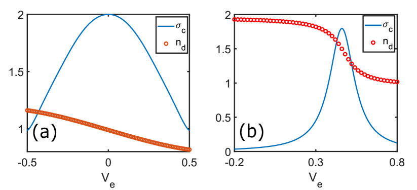
Figure 7: The occupation number $n_{d}$ and the finite bias conductance $\sigma_{c}$ in the Kondo regime (a) $U=1$ and $\Gamma=0.16$ and the double occupation regime (b) $U=0.05$ and $\Gamma=0.04$, where $\varepsilon_{d}=-0.5$ and the hopping amplitude $t_{0}$ is taken as the unit.

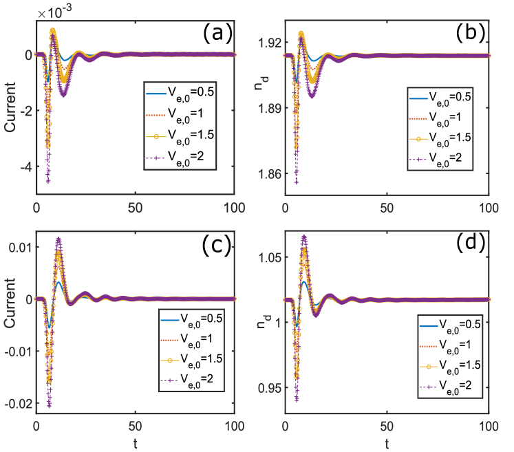
Figure 8: The transient current and the occupation number in the double occupation and Kondo regimes, where $\varepsilon_{d}=-0.5$, $\Gamma=0.04$, $t_{c}=5$, $\alpha=\omega_{d}=1$, and $t_{0}$ is taken as the unit. (a)-(b) $U=0.05$; (c)-(d) $U=1$.

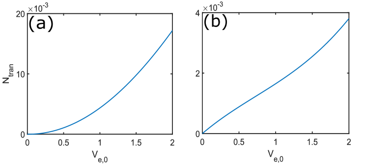
Figure 9: The net transported charge in the double occupation and Kondo regimes, where each lead contains 100 sites, $\varepsilon_{d}=-0.5$, $\Gamma=0.04$, $t_{c}=5$, $\alpha=\omega_{d}=1$, and $t_{0}$ is taken as the unit. (a) $U=0.05$; (b) $U=1$.

For the system with bias time (in)dependent $V_{\mathrm{e}}(t)$, we can study the occupation number $\left\langle n_{d}\right\rangle$, the displacement $\left\langle R\right\rangle$, and the correlation function $C_{\alpha}$. In the non-equilibrium state, the current is defined as $I=\sum_{j,\sigma}\partial_{t}\left\langle c_{j,\sigma,\mathrm{L}}^{\dagger}c_{j,\sigma,\mathrm{L}}\right\rangle$. The Heisenberg equation of motion leads to

$$I = -V\text{Im}\{e_{\lambda}[\left\langle P_{z}(f_{\gamma}^{\dagger}+f_{\gamma})(\gamma c_{0,\uparrow,\mathrm{L}}-c_{0,\downarrow,\mathrm{L}})\right\rangle_{\mathrm{GS}}$$

$$+\left\langle(f_{\gamma}^{\dagger}+f_{\gamma})c_{0,\uparrow,\mathrm{L}}\right\rangle_{\mathrm{GS}}-\gamma\left\langle(f_{\gamma}^{\dagger}-f_{\gamma})c_{0,\downarrow,\mathrm{L}}\right\rangle_{\mathrm{GS}}]\},$$

where the average values depend on the covariance matrix $\Gamma_{m}$ (see Appendix A). The derivatives $\sigma_{c}=\partial_{V_{e}}I$ give the conductance.

IV.2 Transport in the Anderson model

In this subsection, we present results for electron transport in the Anderson model without the electron-phonon interaction. We compute the non-linear conductance in both the Kondo and doubly occupied regimes.

For the Kondo regime we set parameters $(U,\varepsilon_{d},\Gamma)=(1,-0.5,0.16)$ and for the doubly occupied regime we choose $(U,\varepsilon_{d},\Gamma)=(0.05,-0.5,0.04)$, Fig. 7 shows the occupation number $n_{d}$ and the conductance $\sigma_{c}$ in the steady state as the function of $V_{e}$. Fig. 7a shows the conductance $\sigma_{c}$ around zero bias in the Kondo regime. The peak value $\sigma_{c}=2$ originates from the Kondo resonance and agrees with the Friedel sum rule. In the doubly occupied regime, when the bias $V_{\mathrm{e}}$ crosses $\sim\varepsilon_{d}+U$, the energy level of the doubly occupied state in HOMO is higher than the Fermi surface of the right reservoir. As a result, the transport channel is turned on and the electron in HOMO tunnels to the reservoir, resulting in the decay of $n_{d}$ and the appearance of a conductance peak around $\varepsilon_{d}+U$ in Fig. 7b.

In the experiment, an ultrafast pulse is applied to shift the chemical potential of the right lead, where the HOMO is doubly occupied. The effect of the ultrafast pulse centered at the instant $t_{c}$ is described by the time-dependent bias

$$V_{\mathrm{e}}(t)=-V_{\mathrm{e},0}e^{-\alpha^{2}(t-t_{c})^{2}}\sin\omega_{d}(t-t_{c}),$$ (62)

where $V_{\mathrm{e},0}$ is the intensity, $\alpha$ determines the width of the pulse, and $\omega_{d}$ is the frequency.

For different pulse intensities $V_{\mathrm{e},0}$, the transient current $I$ and the occupation number $n_{d}$ as a function of time $t$ are shown in the left and right panels of Fig. 8. The two rows in Fig. 8 correspond to system parameters $(U,\varepsilon_{d})=(0.05,-0.5)$ and $(1,-0.5)$ in the double occupation and Kondo regimes, where $\Gamma=0.04$, $t_{c}=5$, $\alpha=\omega_{d}=1$, and $t_{0}$ is taken as the unit. The number $N_{\mathrm{tran}}$ of electrons transferred from the left lead to the right lead as the function of pulse intensity $V_{e,0}$ is displayed in Fig. 9.

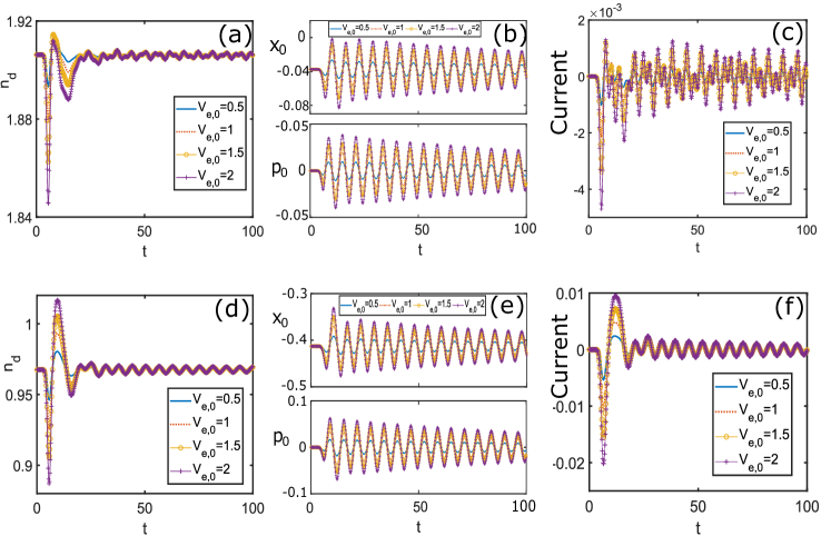
Figure 10: The occupation number (the first column), the average value of the quadrature (the second column), and the transient current (the third column) in the double occupation (the first row) and the Kondo (the second row) regimes, where $\varepsilon_{d}=-0.5$, $\Gamma=0.04$, $g=0.2$, $t_{c}=5$, $\alpha=\omega_{d}=1$, and $t_{0}$ is taken as the unit. (a)-(c): $U=0.05$; (d)-(f): $U=1$.

The pulse has a single period Sine-type shape, which first shifts the Fermi level of the right reservoir downwardly and then lifts it above the Fermi level of the left reservoir after $t_{c}$. In the double occupation regimes, as shown by the first row of Fig. 8, when the Fermi energy is resonant with $\varepsilon_{d}+U<0$ at the instant $t_{\mathrm{res}}<t_{c}$, the transport channel is turned on and the transient current flowing to the right reservoir establishes. However, after the instant $t_{c}$ when the Fermi level of the right reservoir is higher than that of the left reservoir, there is no resonant energy level. Eventually, due to the asymmetric spectral structure around the Fermi level $\varepsilon_{F}=0$, the light pulse induces the non-zero net charge transported $\sim 10^{-2}$ from the left to the right, as shown in Fig. 9a. In the Kondo regime, the energy spectrum is symmetric around the Fermi level, as a result, the net charge transported is highly reduced. We note that a finite value of the net charge $\sim 10^{-3}$ in Fig. 9b most likely arises from the nonlinear electronic dispersion relation in reservoirs.

IV.3 Transport in the Anderson-Holstein model

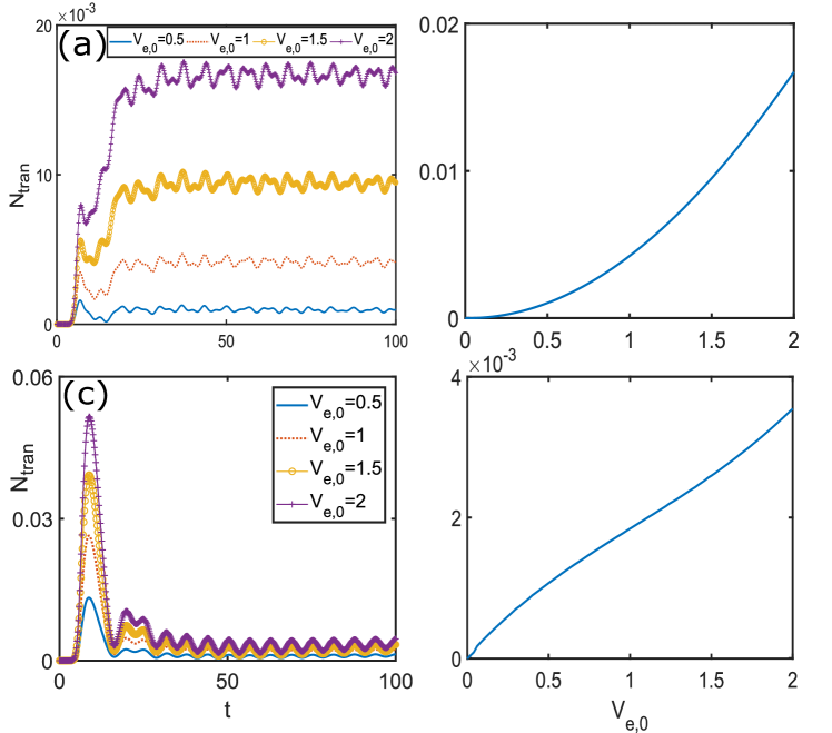
Figure 11: The net charge transport in the double occupation (the first row) and Kondo regimes (the second row), where $\varepsilon_{d}=-0.5$, $\Gamma=0.04$, $g=0.2$, $t_{c}=5$, $\alpha=\omega_{d}=1$, and $t_{0}$ is taken as the unit. (a)-(b): The time-dependent and average value of net charges transport to the right reservoir in the double occupation regime $U=0.05$; (c)-(d): The time-dependent and average value of net charges transport to the right reservoir in the Kondo regime $U=1$.

In this subsection, we concentrate on the phonon excitations generated by the ultrafast pulse in the doubly occupied regime. Since the light pulse induces a transient current, i.e., the transport of electrons between HOMO and leads, the holes are created in the HOMO. The Coulomb interaction between the charge in the substrate and the hole excitation in HOMO induces the molecular vibration after interacting with the ultrafast pulse, which is described by the time-dependent average value $\left\langle R\right\rangle=(x_{0},p_{0})^{T}$ of the quadrature.

In the first and second rows of Fig. 10, we show the occupation number $n_{d}$, the average value $\left\langle R\right\rangle=(x_{0},p_{0})^{T}$ of the quadrature, and the transient current $I$ in the double occupation and Kondo regimes $(U,\varepsilon_{d})=(0.05,-0.5)$ and $(1,-0.5)$, respectively. Here, $\Gamma=0.04$, $g=0.2$, $t_{c}=5$, $\alpha=\omega_{d}=1$, and $t_{0}$ is taken as the unit. The electrons are transferred from the left reservoir to the right one when the terahertz pulse is applied, and the long-lived oscillation of net charge transport around a center value is observed, as shown in the left panel of Fig. 11 for the double occupation and Kondo regimes. Here, the center value of the oscillation as a function of pulse intensity is also shown in the right panel of Fig. 11.

In the initial stage, i.e., $t<t_{c}$, the ultrafast pulse shifts the Fermi level of the right reservoir downwardly, thus electrons in HOMO flow to the right reservoir, and the occupation number $n_{d}$ decreases, as shown in the first column of Fig. 10. Since more holes are generated in the HOMO, the molecule is driven away from the equilibrium position along the negative direction by the electron-phonon interaction, as shown in the second column of Fig. 10. When the Fermi level of the right reservoir is resonant with $\tilde{\varepsilon}_{d}$, the transport channel is turned on, and the significant transient current is formed, as shown in the third column of Fig. 10 and the left panel of Fig. 11.

In the intermediate stage, i.e., $t_{c}<t<t_{c}+\pi/\omega_{d}$, since the Fermi level of the right reservoir is above that of the left one, the HOMO is repumped, as shown in the first column of Fig. 10. However, the resonant transport is absent since the Fermi level of the right reservoir is detuned from LUMO. Eventually, less electrons flow back to the left reservoir, and the finite net charge is transported to the right reservoir, as shown in the Fig. 11. In the final stage $t>t_{c}+\pi/\omega_{d}$, when the light pulse is turned off, the long-lived phonon mode with frequency $\sim\omega_{b}$ survives, as shown in Fig. 10b. Due to the indirect coupling to the reservoir through electrons in HOMO, the phonon mode has a finite life-time, which is revealed by the slowly decaying amplitude of the oscillation in 10b. The molecular vibration induces the long-lived oscillation of current and net charge transport around their values in the steady state, as shown in the third column of Fig. 10 and the left panel of Fig. 11.

IV.4 Discussion of results

Before concluding this section we would like to highlight several results of our analysis.

The main difference between the regimes of single and double occupancy is the dependence of the net transferred charge on the amplitude of the THz light pulse $V_{e,0}$. In the former case we observe a linear dependence of the transferred charge on $V_{e,0}$ (see Fig. 8b), whereas in the latter case we find a non-linear dependence (see Fig. 8a). A special feature of the single occupancy regime is the existence of the Kondo resonance at the Fermi energy, which gives rise to finite DC conductance. This however is not the whole story. In Appendix E we present the analysis of the photoinduced current in the RLM with the energy of the localized state set exactly at the Fermi energy, $\epsilon_{d}=0$, which would also allow for finite DC conductance. In the RLM we also find a non-linear dependence of the photocurrent on $V_{e,0}$ (see fig. 12d). We remind the readers that that the integral of the time dependent electric field in the THz pulse is zero. Hence for a completely linear system the net transferred charge should vanish. The linear dependence of photocurrent on $V_{e,0}$ in the Kondo regime is thus a surprising feature of the system.

Another interesting result of our analysis is the existence of different time scales characterizing the transient dynamics. The occupation number of electrons on the localized orbital exhibits two distinct scales in its dynamics. There is a relatively short timescale over which the strong amplitude deviation from equilibrium configuration decays. It is followed by small amplitude oscillations that match the frequency of the photo-excited phonon mode, with both oscillations of the phonon amplitude and the electron occupation number exhibiting slow decay. The existence of different time scales is a common feature of pump and probe experiments in strongly correlated electron systems (see e.g. Ref. Cao et al. (2018)). Slow relaxation of phonon excitations was one of the key features observed in experiments by Cocker et al. Cocker et al. (2016). Our analysis suggests that the origin of this relaxation is due to phonon displacements modifying virtual tunneling processes of reservoir electrons into the localized orbital, which ultimately allows the phonon energy to be converted into particle-hole excitations.

V Summary and Outlook

We introduced a new method for analyzing the Anderson-Holstein impurity model. Key ingredients of the approach are two unitary transformations that use the parity conservation to partially decouple the impurity degrees of freedom and a generalized polaron transformation to entangle phonons and electrons. An appealing aspect of the new method is that degrees of freedom at very different energy scales, from the local repulsion $U$ to the Kondo temperature $T_{K}$, are described within the same framework and without the numerical demands of the NRG and DMRG calcualtions. To verify the accuracy of the new approach we computed the properties of the Anderson model, including the equilibrium spectral function, linear and non-linear DC conductance. We demonstrated that we correctly reproduce known results for this model. We extended the analysis of the Anderson model to include electron-phonon interactions and showed that it leads to a suppression of the Kondo resonance. We used our approach to analyze THz-STM experiments of tunneling through a single molecule. We found that a picosecond light pulse that induces the current flow gives rise to strong oscillations of the molecular phonon, which persist long after the end of the pulse. We analyzed the time dependence of the current induced by the THz pulse and showed a strong difference between the Kondo and doubly occupied regimes of the molecule.

Our work can be extended in several directions. One interesting question is developing a deeper understanding of the interplay of electron-electron and electron-phonon interactions in pump and probe experiments Yang et al. (2007); Stojchevska et al. (2010); Pomarico et al. (2017); Sch (2008); Schmitt et al. (2011). Recent time-resolved ARPES/Xray experiments by Gerber et al. measured changes of the electron energy relative to the phonon displacement in a photoexcited iron selenide Gerber et al. (2017). They observed a strong renormalization of the electron-phonon coupling relative to the value predicted from band structure calculations and attributed it to the effects of electron-electron interactions. Extension of the formalism presented in this paper can be used to study the time dependent spectral function of electrons following a THz light pulse. This analysis will provide a direct comparison between changes of the electron energy and the phonon amplitude.

Another interesting question is the analysis of shot to shot fluctuations in the number of electrons transferred through the junction during the THz pulse. In the case of DC transport the study of shot noise has been a valuable tool for understanding underlying many-body states (see Refs. Nazarov (2003); Blanter and Buttiker (2000); Beenakker and Sch (2003) for a review), including the demonstration of fractional statistics in the fractional quantum Hall states Kane and Fisher (1993); Reznikov et al. (2002) and understanding the back-scattering mechanism in the Kondo system Sela et al. (2006); Golub (2006); Yamauchi et al. (2011) as a probe of the low temperature fixed point.

The formalism developed in our paper introduces a powerful new technique that can be used for the theoretical analysis of many different types of nonequilibrium problems. For example, it should provide useful insights into the analysis of resonant XRay scattering experiments Ament et al. (2011) in materials with mobile electrons. The essence of these experiments is that an incident photon excites an electron from the core orbital into one of the unoccupied bands, which results in a sudden introduction of a positively charged hole in the sea of conduction band electronsBenjamin et al. (2013). The attractive potential of the hole is strong enough to allow the formation of the excitonic bound state, however, such bound state can be occupied by only one of the electrons. Hence, an analysis of the many-body dynamics following absorption of the incident photon should include the local repulsion on the hole site. The formalism developed in this paper can be used for computing RIXS processes involving the excitation of bosonic modes, such as phonons and magnons, as well as a continuum of electron-hole pairs. Another interesting direction for applying the ideas presented in this paper is to use variational non-Gaussian states as a solver for non-equilibrium DMFT calculations Aoki et al. (2014); Ganahl et al. (2015).

VI Acknowledgements

We are grateful for useful discussions with D. Abanin, Y. Ashida, T. Cocker, A. Georges, L. Glazman, M. Kanasz-Nagy, A. Lichtenstein, A. Millis, A. Rosch, A. Rubtsov, Z.X. Shen, J. van den Brink, G. Zarand. T. S. acknowledges the Thousand-Youth-Talent Program of China. J.I.C acknowledges the ERC Advanced Grant QENOCOBA under the EU Horizon2020 program (grant agreement 742102) and the German Research Foundation (DFG) under Germany’s Excellence Strategy through Project No. EXC-2111-390814868 (MCQST) and within the D-A-CH Lead-Agency Agreement through project No. 414325145 (BEYOND C). ED acknowledges support from the Harvard-MIT CUA, Harvard-MPQ Center, AFOSR-MURI: Photonic Quantum Matter (award FA95501610323), and DARPA DRINQS program (award D18AC00014).

Appendix A Mean-field Hamiltonian of fermions

The Wick-theorem gives the mean-field Hamiltonian

$$\mathcal{H}_{m}=-i\frac{1}{2}W_{f}\left(\begin{array}[]{cc}\mathcal{E}_{0}&\Delta_{0}\\ \Delta_{0}^{\dagger}&-\mathcal{E}_{0}^{T}\end{array}\right)W_{f}^{\dagger}+\mathcal{H}_{m}^{P},$$ (63)

in the Majorana basis, where the matrices

$$\mathcal{E}_{0} = \frac{1}{2}\left(\begin{array}[]{ccc}\tilde{U}&v_{-}&v_{-}\\ v_{-}^{\dagger}&2h_{\mathrm{L}}&0\\ v_{-}^{\dagger}&0&2h_{\mathrm{R}}\end{array}\right),\Delta_{0}=\frac{1}{2}\left(\begin{array}[]{ccc}0&-v_{+}&-v_{+}\\ v_{+}^{T}&0&0\\ v_{+}^{T}&0&0\end{array}\right),$$ (70)

$$\mathcal{E}_{P} = \frac{1}{2}\gamma\left(\begin{array}[]{ccc}U_{P}&v_{-}&v_{-}\\ -v_{+}^{T}&0&0\\ -v_{+}^{T}&0&0\end{array}\right),\Delta_{P}=\frac{1}{2}\gamma\left(\begin{array}[]{ccc}0&v_{-}&v_{-}\\ 0&0&0\\ 0&0&0\end{array}\right)$$ (77)

are defined by $U_{P}=\tilde{U}+2\tilde{\varepsilon}_{d}-2\Delta_{R}^{T}G_{\lambda}$, the vectors $v_{\pm}=V\left\langle e^{\mp iR^{T}\lambda}\right\rangle_{\mathrm{GS}}(1,\pm\gamma)\otimes(1,0_{N-1})$, and the hopping matrices $h_{\mathrm{a}=\mathrm{L,R}}=I_{2}\otimes(-t_{0}\delta_{i,j\pm 1}-\mu_{\mathrm{a}}\delta_{ij})$ in the left and right reservoirs. The matrix $\mathcal{H}_{m}^{P}=4\delta E_{P}/\delta\Gamma_{m}$ is determined by the derivative of $E_{P}=\left\langle P_{z}c^{\dagger}\mathcal{E}_{P}c\right\rangle+2$Re$\left\langle P_{z}c^{T}\Delta_{P}c\right\rangle$.

The $2\times 2$ Gram matrix

$$\mathbf{G} = \left\langle P_{c}P_{c}\right\rangle\Gamma_{b}+\left\langle P_{h}P_{h}\right\rangle(4\sigma^{y}\lambda\lambda^{T}\sigma^{y}$$ (78)

$$+\Delta_{R}\Delta_{R}^{T}+2i\Delta_{R}\lambda^{T}\sigma^{y}-2i\sigma^{y}\lambda\Delta_{R}^{T})$$

of the tangential vector $U_{\mathrm{ph}}U_{\mathrm{A}}U_{\mathrm{GS}}V_{h}\left|0\right\rangle$ is determined by

$$\left\langle P_{c}P_{c}\right\rangle = \left\langle f_{\gamma}^{\dagger}f_{\gamma}\right\rangle_{\mathrm{GS}}-\left\langle P_{z}f_{\gamma}^{\dagger}f_{\gamma}\right\rangle_{\mathrm{GS}}^{2},$$

$$\left\langle P_{h}P_{h}\right\rangle = \left\langle P_{c}P_{c}\right\rangle-\frac{1}{2}\left\langle P_{z}f_{\gamma}^{\dagger}f_{\gamma}\text{:}C^{\dagger}O_{P}C\text{:}\right\rangle_{\mathrm{GS}}.$$ (79)

The vector

$$\xi_{\tau} = i(\Gamma_{b}-\sigma^{y})(\left\langle P_{c}P_{c}\right\rangle G_{\lambda}-\gamma\Sigma_{c}\lambda)$$ (80)

$$-(2\sigma^{y}\lambda+i\Delta_{R})(\frac{1}{2}U_{P}\left\langle f_{\gamma}^{\dagger}f_{\gamma}\right\rangle_{\mathrm{GS}}+\gamma\Sigma_{h})$$

is the overlap of the tangential vector and the right hide side of Eq. (30), where

$$\Sigma_{c} = i\frac{V}{2}\sum_{\mathrm{a}}[e_{\lambda}\left\langle(1+\gamma P_{z})f_{\gamma}^{\dagger}(\gamma c_{0,\uparrow,\mathrm{a}}-c_{0,\downarrow,\mathrm{a}})\right\rangle_{\mathrm{GS}}$$

$$+e_{\lambda}^{\ast}\left\langle(1-\gamma P_{z})(\gamma c_{0,\uparrow,\mathrm{a}}^{\dagger}+c_{0,\downarrow,\mathrm{a}}^{\dagger})f_{\gamma}^{\dagger}\right\rangle_{\mathrm{GS}}]$$

$$+\left\langle P_{z}f_{\gamma}^{\dagger}f_{\gamma}\right\rangle_{\mathrm{GS}}\text{Im}\left\langle\mathcal{I}_{dc}\right\rangle_{\mathrm{GS}},$$

$$\Sigma_{h} = \frac{1}{2}V\sum_{\mathrm{a}}[e_{\lambda}\left\langle f_{\gamma}^{\dagger}(\gamma c_{0,\uparrow,\mathrm{a}}-c_{0,\downarrow,\mathrm{a}})\right\rangle_{\mathrm{GS}}$$

$$-e_{\lambda}^{\ast}\left\langle(\gamma c_{0,\uparrow,\mathrm{a}}^{\dagger}+c_{0,\downarrow,\mathrm{a}}^{\dagger})f_{\gamma}^{\dagger}\right\rangle_{\mathrm{GS}}]$$

$$-E_{P}\left\langle P_{z}f_{\gamma}^{\dagger}f_{\gamma}\right\rangle_{\mathrm{GS}}-\frac{1}{2}\left\langle P_{z}f_{\gamma}^{\dagger}f_{\gamma}\text{:}C^{\dagger}\mathcal{H}_{f}^{P}C\text{:}\right\rangle_{\mathrm{GS}},$$

and $\mathcal{H}_{f}^{P}=iW_{f}^{\dagger}\mathcal{H}_{m}^{P}W_{f}/2$ is the matrix in the Nambu basis.

The mean-field Hamiltonian, the Gram matrix, and the vector $\xi_{\tau}$ involve the average values $\left\langle P_{z}\right\rangle_{\mathrm{GS}}$, $\left\langle P_{z}C_{i}C_{j}^{\dagger}\right\rangle_{\mathrm{GS}}$ and $\left\langle P_{z}f_{\gamma}^{\dagger}f_{\gamma}C_{i}^{\dagger}C_{j}\right\rangle_{\mathrm{GS}}$ on the Gaussian state. We consider the average values of operators $P_{z}^{\theta}=e^{\theta f^{\dagger}f}P_{z}$ and $P_{z}^{\theta}C_{i}C_{j}^{\dagger}$, which eventually give $\left\langle P_{z}\right\rangle_{\mathrm{GS}}=\left\langle P_{z}^{\theta=0}\right\rangle$ and $\left\langle P_{z}C_{i}C_{j}^{\dagger}\right\rangle_{\mathrm{GS}}=\left\langle P_{z}^{\theta=0}C_{i}C_{j}^{\dagger}\right\rangle_{\mathrm{GS}}$, as well as $\left\langle P_{z}f_{\gamma}^{\dagger}f_{\gamma}C_{i}^{\dagger}C_{j}\right\rangle_{\mathrm{GS}}$ by the derivative $\left.\partial_{\theta}\left\langle P_{z}^{\theta}C_{i}C_{j}^{\dagger}\right\rangle_{\mathrm{GS}}\right|_{\theta=0}$.

As shown in Ref. Shi et al. (2018); Ashida et al. (2018a), the average values $\left\langle P_{z}^{\theta}\right\rangle_{\mathrm{GS}}=-$Pf$(\Gamma_{F}/2)$ and

$$\left\langle P_{z}^{\theta}c_{l}^{\dagger}c_{k}\right\rangle_{\mathrm{GS}} = \frac{1}{4}\left\langle P_{z}^{\theta}\right\rangle_{\mathrm{GS}}[\left(1,i\right)\mathcal{S}\Theta\left(\begin{array}[]{c}1\\ -i\end{array}\right)]_{kl},$$ (85)

$$\left\langle P_{z}^{\theta}c_{l}c_{k}\right\rangle_{\mathrm{GS}} = -\frac{1}{4}\left\langle P_{z}^{\theta}\right\rangle_{\mathrm{GS}}[(1,i)\mathcal{S}\left(\begin{array}[]{c}1\\ i\end{array}\right)]_{kl},$$ (88)

are determined by the Pfaffian of

$$\Gamma_{F}=\sqrt{1+\Theta}\Gamma_{m}\sqrt{1+\Theta}-\sigma(1-\Theta),$$ (89)

$\mathcal{S}=(\sigma\Gamma_{m}-1)\mathcal{T}$, and

$$\mathcal{T}=\frac{1}{1+\frac{1}{2}(1+\Theta)(\sigma\Gamma_{m}-1)},$$ (90)

where $\Theta=I_{2}\otimes\sigma_{\theta}$, $\sigma_{\theta}=diag(-e^{\theta},1_{1\times N},-1_{1\times N},1_{1\times N},-1_{1\times N})$ is a diagonal matrix and

$$\sigma=\left(\begin{array}[]{cc}{0}&{\openone}_{4N+1}\\ -{\openone}_{4N+1}&0\end{array}\right)$$ (91)

is a symplectic matrix. The anti-commutation relation results in

$$\left\langle P_{z}^{\theta=0}c_{l}c_{k}^{\dagger}\right\rangle_{\mathrm{GS}} = \left\langle P_{z}^{0}\right\rangle\delta_{lk}-\left\langle P_{z}^{0}c_{k}^{\dagger}c_{l}\right\rangle,$$

$$\left\langle P_{z}^{\theta=0}c_{l}^{\dagger}c_{k}^{\dagger}\right\rangle_{\mathrm{GS}} = (\sigma_{0})_{kk}[\left\langle P_{z}^{0}c_{k}c_{l}\right\rangle]^{\ast}(\sigma_{0})_{ll}.$$ (92)

By the derivative to $\theta$ and taking the limit $\theta\rightarrow 0$, we obtain

$$\left\langle P_{z}f_{\gamma}^{\dagger}f_{\gamma}c_{i}^{\dagger}c_{j}\right\rangle=-\frac{1}{2}g_{F}\left\langle P_{z}c_{i}^{\dagger}c_{j}\right\rangle_{\mathrm{GS}}-\frac{1}{4}\left\langle P_{z}\right\rangle_{\mathrm{GS}}[\left(1,i\right)\mathcal{S}w(1-\frac{1}{2}\mathcal{S}\Theta)\left(\begin{array}[]{c}1\\ -i\end{array}\right)]_{ji},$$ (93)

and

$$\left\langle P_{z}f_{\gamma}^{\dagger}f_{\gamma}c_{i}c_{j}\right\rangle=-\frac{1}{2}g_{F}\left\langle P_{z}c_{i}c_{j}\right\rangle_{\mathrm{GS}}-\frac{1}{8}\left\langle P_{z}\right\rangle_{\mathrm{GS}}[(1,i)\mathcal{S}w\mathcal{S}\left(\begin{array}[]{c}1\\ i\end{array}\right)]_{ji},$$ (94)

where $w=I_{2}\otimes diag(1,0_{1\times 4N})$ and

$$g_{F}=tr(\Gamma_{F}^{-1}\sigma w+\frac{1}{2}\mathcal{T}\sigma w\Gamma_{m}).$$ (95)

The commutation relation leads to

$$\left\langle P_{z}f_{\gamma}^{\dagger}f_{\gamma}c_{i}c_{j}^{\dagger}\right\rangle_{\mathrm{GS}} = \left\langle P_{z}f_{\gamma}^{\dagger}f_{\gamma}\right\rangle_{\mathrm{GS}}\delta_{ij}-\left\langle P_{z}f_{\gamma}^{\dagger}f_{\gamma}c_{j}^{\dagger}c_{i}\right\rangle_{\mathrm{GS}},$$

$$\left\langle P_{z}f_{\gamma}^{\dagger}f_{\gamma}c_{i}^{\dagger}c_{j}^{\dagger}\right\rangle_{\mathrm{GS}} = (\sigma_{\theta})_{ii}\left\langle P_{z}f_{\gamma}^{\dagger}f_{\gamma}c_{j}c_{i}\right\rangle^{\ast}(\sigma_{\theta})_{jj}$$ (96)

$$+\delta_{i1}\left\langle P_{z}f_{\gamma}^{\dagger}c_{j}^{\dagger}\right\rangle-\left\langle P_{z}f_{\gamma}^{\dagger}c_{i}^{\dagger}\right\rangle\delta_{j1}.$$

The mean-field Hamiltonian $\mathcal{H}_{m}^{P}$ is determined by the derivatives

$$\frac{\delta}{\delta\Gamma_{m,ij}}\left\langle P_{z}\right\rangle_{\mathrm{GS}}=-\frac{1}{2}\left\langle P_{z}\right\rangle_{\mathrm{GS}}\sqrt{1+\Theta}\frac{1}{\Gamma_{F}}\sqrt{1+\Theta},$$ (97)

$$\frac{\delta}{\delta\Gamma_{m,ij}}\left\langle P_{z}c_{l}^{\dagger}c_{k}\right\rangle_{\mathrm{GS}} = -\frac{1}{2}\left\langle P_{z}c_{l}^{\dagger}c_{k}\right\rangle_{\mathrm{GS}}(\sqrt{1+\Theta}\frac{1}{\Gamma_{F}}\sqrt{1+\Theta})_{ij}$$ (100)

$$-i\frac{1}{4}\left\langle P_{z}\right\rangle_{\mathrm{GS}}[\mathcal{T}\Theta\left(\begin{array}[]{c}1\\ -i\end{array}\right)]_{jl}[\left(1,i\right)\mathcal{T}^{T}]_{ki},$$

and

$$\frac{\delta}{\delta\Gamma_{m,ij}}\left\langle P_{z}c_{l}c_{k}\right\rangle = -\frac{1}{2}\left\langle P_{z}c_{l}c_{k}\right\rangle_{\mathrm{GS}}(\sqrt{1+\Theta}\frac{1}{\Gamma_{F}}\sqrt{1+\Theta})_{ij}$$ (103)

$$+i\frac{1}{4}\left\langle P_{z}\right\rangle_{\mathrm{GS}}[\mathcal{T}\left(\begin{array}[]{c}1\\ i\end{array}\right)]_{jl}[(1,i)\mathcal{T}^{T}]_{ki}.$$

Appendix B Linearized ODE for $\partial_{\tau}\lambda$

In this section, we reduce EOM (43), i.e.,

$$\partial_{\tau}\lambda^{T}\mathbf{M}\partial_{\tau}\lambda=\partial_{\tau}\lambda^{T}\xi_{\tau}.$$ (104)

to the linear ODE, where $\xi_{\tau}=(\xi_{\tau,x},\xi_{\tau,p})^{T}$ and

$$\mathbf{M=}\left(\begin{array}[]{cc}\mathbf{M}_{11}&\mathbf{M}_{12}\\ \mathbf{M}_{21}&\mathbf{M}_{22}\end{array}\right).$$ (105)

Since the left hand side of Eq. (43) is always real, the imaginary part of $\partial_{\tau}\lambda^{T}\xi_{\tau}$ must vanish, which gives rise to

$$\partial_{\tau}\lambda_{x}\text{Im}\xi_{\tau,x}+\partial_{\tau}\lambda_{p}\text{Im}\xi_{\tau,p}=0\text{.}$$ (106)

Four possibilities may happen: (a) Im$\xi_{\tau,x}=$Im$\xi_{\tau,p}=0$; (b) Im$\xi_{\tau,x}=0$, Im$\xi_{\tau,p}\neq 0$; (c) Im$\xi_{\tau,x}\neq 0$, Im$\xi_{\tau,p}=0$; (d) Im$\xi_{\tau,x}\neq 0$, Im$\xi_{\tau,p}\neq 0$.

For the case (a), EOM (43) is reduced to $\mathbf{M}\partial_{\tau}\lambda=\xi_{\tau}$. For the case (b), EOM (43) becomes

$$\partial_{\tau}\lambda_{p}=0,\mathbf{M}_{11}\partial_{\tau}\lambda_{x}=\xi_{\tau,x}.$$ (107)

For the case (c), EOM (43) is

$$\partial_{\tau}\lambda_{x}=0,\mathbf{M}_{22}\partial_{\tau}\lambda_{p}=\xi_{\tau,p}.$$ (108)

For the last case, EOM (43) reads

$$\partial_{\tau}\lambda_{p} = -\frac{\text{Im}\xi_{\tau,x}}{\text{Im}\xi_{\tau,p}}\partial_{\tau}\lambda_{x},$$

$$\partial_{\tau}\lambda_{x} = \frac{1}{v_{\xi}^{T}\mathbf{M}v_{\xi}}v_{\xi}^{T}\xi_{\tau},$$ (109)

where the vector $v_{\xi}=(1,-$Im$\xi_{\tau,x}/$Im$\xi_{\tau,p})^{T}$.

Appendix C Eveluation of average values in $G_{R}(t)$

In this Appendix, we calculate the average values in the retarded Green function $G_{R}(t)$, which are

$$\left\langle e^{-iR^{T}(t)\lambda}e^{iR^{T}\lambda}\right\rangle_{\mathrm{GS}},\left\langle e^{iR^{T}\lambda}e^{-iR^{T}(t)\lambda}\right\rangle_{\mathrm{GS}}$$ (110)

for the phonon and

$$\left\langle F(t)F^{\dagger}\right\rangle_{\mathrm{GS}},\left\langle F^{\dagger}F(t)\right\rangle_{\mathrm{GS}}$$ (111)

for fermions.

We first consider the phonon part. The average value

$$\left\langle e^{-iR^{T}(t)\lambda}e^{iR^{T}\lambda}\right\rangle_{\mathrm{GS}}=\text{ }_{b}\left\langle\bar{\Psi}_{\mathrm{GS}}\right|e^{-i\omega_{\mathrm{re}}tb^{\dagger}b}\left|\bar{\Psi}_{\mathrm{GS}}\right\rangle_{b}$$ (112)

can be rewritten as the mean value of $e^{-i\omega_{\mathrm{re}}b^{\dagger}bt}$ on the normalized Gaussian state

$$\left|\bar{\Psi}_{\mathrm{GS}}\right\rangle_{b}=e^{iR^{T}S_{p}^{T}\lambda}\left|0\right\rangle_{b},$$ (113)

where the symplectic matrix $S_{p}$ diagonalizes the phonon mean-field Hamiltonian $\Omega_{\mathrm{re}}$ as $S_{p}^{T}\Omega_{\mathrm{re}}S_{p}=\omega_{\mathrm{re}}I_{2}$.

The Gaussian state $\left|\bar{\Psi}_{\mathrm{GS}}\right\rangle_{b}$ is fully characterized by the average value $\Delta_{\lambda}=-2S_{p}^{-1}i\sigma^{y}\lambda$ of quadrature and the covariance matrix $\bar{\Gamma}_{b}=I$. The average value

$$\left\langle e^{-iR^{T}(t)\lambda}e^{iR^{T}\lambda}\right\rangle_{\mathrm{GS}}=e^{-\frac{1}{4}\Delta_{\lambda}^{T}\Delta_{\lambda}(1-e^{-i\omega_{\mathrm{re}}t})}.$$ (114)

follows from the result in Ref. Shi et al. (2018). Following the similar procedure, one can obtain $\left\langle e^{iR^{T}\lambda}e^{-iR^{T}(t)\lambda}\right\rangle_{\mathrm{GS}}$.

We analyze the fermionic part in the next step. The average value

$$\left\langle F(t)F^{\dagger}\right\rangle_{\mathrm{GS}} = \frac{1}{4}[u_{-}^{T}g_{1}(t)u_{-}+\gamma u_{-}^{T}g_{2}(t)u_{+}$$ (115)

$$+\gamma u_{+}^{T}g_{3}(t)u_{-}+g_{4}(t)]$$

contains four terms $g_{1}(t)=\left\langle C(t)C^{\dagger}\right\rangle_{\mathrm{GS}}$, $g_{2}(t)=\left\langle C(t)P_{z}C^{\dagger}\right\rangle_{\mathrm{GS}}$, $g_{3}(t)=\left\langle P_{z}C(t)C^{\dagger}\right\rangle_{\mathrm{GS}}$, and

$$g_{4}(t)=\left\langle P_{z}(f+f^{\dagger})(t)P_{z}(f+f^{\dagger})\right\rangle_{\mathrm{GS}},$$ (116)

where $u_{\pm}^{T}=(1,\pm 1)\otimes(1,0_{2N})$.

It follows from the Heisenberg equations of motion that the first three terms obey

$$i\partial_{t}g_{1,2}(t) = \mathcal{H}_{f}g_{1,2}(t),$$

$$i\partial_{t}g_{3}(t) = g_{3}(t)\mathcal{H}_{f},$$ (117)

where $\mathcal{H}_{f}=iW_{f}^{\dagger}\mathcal{H}_{m}W_{f}/2$. The solutions

$$g_{1,2}(t) = e^{-i\mathcal{H}_{f}t}g_{1,2}(0),$$

$$g_{3}(t) = g_{3}(0)e^{-i\mathcal{H}_{f}t},$$ (118)

are determined by the boundary values $g_{1}(0)=\left\langle CC^{\dagger}\right\rangle_{\mathrm{GS}}$, $g_{2}=\left\langle CP_{z}C^{\dagger}\right\rangle_{\mathrm{GS}}$, and $g_{3}(0)=\left\langle P_{z}CC^{\dagger}\right\rangle_{\mathrm{GS}}$ are obtained analytically in Appendix A.

Applying the parity operator on the mean-field Hamiltonian, we can write the fourth term

$$g_{4}(t)=e^{iE_{\mathrm{MF}}^{e}t}\text{ }_{f}\left\langle\Psi_{\mathrm{GS}}\right|(f_{\gamma}+f_{\gamma}^{\dagger})e^{-i\frac{1}{2}C^{\dagger}\mathcal{H}_{\Theta}Ct}(f_{\gamma}+f_{\gamma}^{\dagger})\left|\Psi_{\mathrm{GS}}\right\rangle_{f}$$ (119)

by $\mathcal{H}_{\Theta}=\Theta\mathcal{H}_{f}\Theta$, where $H_{\mathrm{MF}}^{e}\left|\Psi_{\mathrm{GS}}\right\rangle_{f}=E_{\mathrm{MF}}^{e}\left|\Psi_{\mathrm{GS}}\right\rangle_{f}$. Introducing the unitary transformation $V_{\Theta}$: $V_{\Theta}^{\dagger}CV_{\Theta}=U_{\Theta}C$, we obtain

$$g_{4}(t)=e^{i\bar{\epsilon}t}\text{ }_{f}\left\langle\bar{\Psi}_{\mathrm{GS}}\right|e^{-ic^{\dagger}\epsilon ct}\left|\bar{\Psi}_{\mathrm{GS}}\right\rangle_{f}$$ (120)

where $\bar{\epsilon}=E_{\mathrm{MF}}^{e}+tr\epsilon/2$, $U_{\Theta}$ diagonalizes the matrix $\mathcal{H}_{\Theta}$ as

$$U_{\Theta}^{\dagger}\mathcal{H}_{\Theta}U_{\Theta}=D=\left(\begin{array}[]{cc}\epsilon&0\\ 0&-\epsilon\end{array}\right),\epsilon_{j}\geq 0,$$ (121)

and $\left|\bar{\Psi}_{\mathrm{GS}}\right\rangle_{f}=V_{\Theta}^{\dagger}(f_{\gamma}+f_{\gamma}^{\dagger})\left|\Psi_{\mathrm{GS}}\right\rangle_{f}$ is a normalized Gaussian state.

The Gaussian state $\left|\bar{\Psi}_{\mathrm{GS}}\right\rangle_{f}$ is fully characterized by the covariance matrix

$$\bar{\Gamma}_{f} = \text{ }_{f}\left\langle\bar{\Psi}_{\mathrm{GS}}\right|CC^{\dagger}\left|\bar{\Psi}_{\mathrm{GS}}\right\rangle_{f}$$ (122)

$$= U_{\Theta}^{\dagger}[(\sigma_{x}\Gamma_{f}u_{+}u_{+}^{T}\Gamma_{f}\sigma_{x})^{T}-\Gamma_{f}u_{+}u_{+}^{T}\Gamma_{f}+\Gamma_{f}]U_{\Theta}.$$

It follows from the result in Ref. that

$$g_{4}(t)=-e^{i\bar{\epsilon}t}\text{Pf}(\frac{\bar{\Gamma}_{F}}{2}),$$ (123)

where

$$\bar{\Gamma}_{F}=\sqrt{1-e^{-i\epsilon t}}\bar{\Gamma}_{m}\sqrt{1-e^{-i\epsilon t}}-\sigma(1+e^{-i\epsilon t})$$ (124)

is determined by $\bar{\Gamma}_{m}=i(W_{f}\bar{\Gamma}_{f}W_{f}^{\dagger}-1)$. Following the same procedure, one can also obtain the average value $\left\langle F^{\dagger}F(t)\right\rangle_{\mathrm{GS}}$.

Appendix D Mean-field Hamiltonian of penalty term

In this Appendix, we derive the mean-field Hamiltonian of the penalty term $H_{\Lambda}$ by the Wick theorem. In the explicit form, the Hamiltonian

$$H_{\Lambda}/\Lambda = (1-2\bar{N}_{\uparrow})\sum_{j,a}c_{j,\uparrow,a}^{\dagger}c_{j,\uparrow,a}+(\sum_{ia}c_{i,\uparrow,a}^{\dagger}c_{i,\uparrow,a})^{2}$$ (125)

$$+(1-2\bar{N}_{\downarrow})\sum_{i,a}c_{i,\downarrow,a}^{\dagger}c_{i,\downarrow,a}+(\sum_{i,a}c_{i,\downarrow,a}^{\dagger}c_{i,\downarrow,a})^{2}$$

$$+(\bar{N}_{\downarrow}-\bar{N}_{\uparrow})\gamma P_{z}+\gamma P_{z}c^{\dagger}\mathcal{E}_{P}^{\mu}c+2\gamma\sum_{j,a}P_{z}f_{\gamma}^{\dagger}f_{\gamma}c_{j,\downarrow,a}^{\dagger}c_{j,\downarrow,a}$$

$$+\bar{N}_{\uparrow}^{2}+\bar{N}_{\downarrow}^{2}-\bar{N}_{\uparrow}-\bar{N}_{\downarrow}+1,$$

where the matrix

$$\mathcal{E}_{P}^{\mu}=\left(\begin{array}[]{ccc}1-2\bar{N}_{\downarrow}&0&0\\ 0&(\delta_{\sigma\uparrow}-\delta_{\sigma\downarrow})\delta_{\sigma\sigma^{\prime}}\delta_{ij}&0\\ 0&0&(\delta_{\sigma\uparrow}-\delta_{\sigma\downarrow})\delta_{\sigma\sigma^{\prime}}\delta_{ij}\end{array}\right).$$ (126)

The Wick theorem gives the mean-field Hamiltonian $H_{\Lambda,\mathrm{MF}}=i$:$A^{T}\mathcal{H}_{\Lambda,m}A$:$/4$, where

$$\mathcal{H}_{\Lambda,m}/\Lambda=-i\frac{1}{2}W_{f}\left(\begin{array}[]{cc}\mathcal{E}_{\mu}&\Delta_{\mu}\\ \Delta_{\mu}^{\dagger}&-\mathcal{E}_{\mu}\end{array}\right)W_{f}^{\dagger}+4\frac{\delta E_{P}^{\mu}}{\delta\Gamma_{m}}$$ (127)

is determined by

$$\mathcal{E}_{\mu} = 2\delta_{ab}[(1-\bar{N}_{\uparrow}+\sum_{lc}\left\langle c_{l,\uparrow,c}^{\dagger}c_{l,\uparrow,c}\right\rangle_{\mathrm{GS}})\delta_{\sigma\uparrow}$$ (128)

$$+(1-\bar{N}_{\downarrow}+\sum_{lc}\left\langle c_{l,\downarrow,c}^{\dagger}c_{l,\downarrow,c}\right\rangle_{\mathrm{GS}})\delta_{\sigma\downarrow}]\delta_{\sigma\sigma^{\prime}}\delta_{ij}$$

$$-2(\left\langle c_{j,\uparrow,b}^{\dagger}c_{i,\uparrow,a}\right\rangle_{\mathrm{GS}}\delta_{\sigma\uparrow}+\left\langle c_{j,\downarrow,b}^{\dagger}c_{i,\downarrow,a}\right\rangle_{\mathrm{GS}}\delta_{\sigma\downarrow})\delta_{\sigma\sigma^{\prime}},$$

$$\Delta_{\mu}=2(\left\langle c_{j,\uparrow,b}c_{i,\uparrow,a}\right\rangle_{\mathrm{GS}}\delta_{\sigma\uparrow}+\left\langle c_{j,\downarrow,b}c_{i,\downarrow,a}\right\rangle_{\mathrm{GS}}\delta_{\sigma\downarrow})\delta_{\sigma\sigma^{\prime}},$$ (129)

and

$$E_{P}^{\mu}=(\bar{N}_{\downarrow}-\bar{N}_{\uparrow})\gamma\left\langle P_{z}\right\rangle_{\mathrm{GS}}+\gamma\left\langle P_{z}c^{\dagger}\mathcal{E}_{P}^{\mu}c\right\rangle_{\mathrm{GS}}+2\gamma\sum_{j,a}\left\langle P_{z}f_{\gamma}^{\dagger}f_{\gamma}c_{j,\downarrow,a}^{\dagger}c_{j,\downarrow,a}\right\rangle_{\mathrm{GS}}.$$ (130)

The derivatives to the covariance matrix are given by Eqs. (97)-(103) and

$$4\frac{\delta}{\delta\Gamma_{m,ij}}\left\langle P_{z}f_{\gamma}^{\dagger}f_{\gamma}c_{l}^{\dagger}c_{k}\right\rangle_{\mathrm{GS}}$$ (140)

$$= -2\left\langle P_{z}f_{\gamma}^{\dagger}f_{\gamma}c_{l}^{\dagger}c_{k}\right\rangle(\sqrt{1+\Theta}\frac{1}{\Gamma_{F}}\sqrt{1+\Theta})_{ij}-2\left\langle P_{z}c_{l}^{\dagger}c_{k}\right\rangle_{\mathrm{GS}}\partial_{\theta}(\sqrt{1+\Theta}\frac{1}{\Gamma_{F}}\sqrt{1+\Theta})_{ij}$$

$$+i\left\langle P_{z}\right\rangle_{\mathrm{GS}}\{\frac{1}{2}g_{F}[\mathcal{T}\Theta\left(\begin{array}[]{c}1\\ -i\end{array}\right)]_{jl}[\left(1,i\right)\mathcal{T}^{T}]_{ki}-[\frac{1}{2}\mathcal{T}w(\sigma\Gamma_{m}-1)\mathcal{T}\Theta\left(\begin{array}[]{c}1\\ -i\end{array}\right)]_{jl}[\left(1,i\right)\mathcal{T}^{T}]_{ki}$$

$$+[\mathcal{T}w\left(\begin{array}[]{c}1\\ -i\end{array}\right)]_{jl}[\left(1,i\right)\mathcal{T}^{T}]_{ki}-\frac{1}{2}[\mathcal{T}\Theta\left(\begin{array}[]{c}1\\ -i\end{array}\right)]_{jl}[\left(1,i\right)\mathcal{T}^{T}(\Gamma_{m}\sigma-1)w\mathcal{T}^{T}]_{ki}\},$$

where

$$\partial_{\theta}(\sqrt{1+\Theta}\frac{1}{\Gamma_{F}}\sqrt{1+\Theta})$$ (141)

$$= -\frac{1}{4}w\sigma\mathcal{T}^{T}-\frac{1}{4}\mathcal{T}\sigma w+\frac{1}{4}\mathcal{T}\sigma w\Gamma_{m}\sqrt{1+\Theta}\frac{1}{\Gamma_{F}}\sqrt{1+\Theta}$$

$$+\frac{1}{4}\sqrt{1+\Theta}\frac{1}{\Gamma_{F}}\sqrt{1+\Theta}\Gamma_{m}w\sigma\mathcal{T}^{T}+\sqrt{1+\Theta}\frac{1}{\Gamma_{F}}\sigma w\frac{1}{\Gamma_{F}}\sqrt{1+\Theta}.$$

Appendix E Ultrafast processes in RLM

In this Appendix, we consider phototransport in the resonant level model in the so-called infinite bandwidth limit (see ref Cuevas and Scheer (1990) for details). The system Hamiltonian is given by

$$H_{\mathrm{RLM}}=\sum_{k,\mathrm{a}}(k-\mu_{\mathrm{a}})c_{k,\mathrm{a}}^{\dagger}c_{k,\mathrm{a}}+\varepsilon_{d}d^{\dagger}d+\frac{V}{\sqrt{L}}\sum_{k,\mathrm{a}}(c_{k,\mathrm{a}}^{\dagger}d+\mathrm{H.c.}),$$ (142)

where we set $v_{\mathrm{F}}=1$, the chemical potential of the left lead is fixed $\mu_{\mathrm{L}}=0$, and the effect of the ultrafast light is described by $\mu_{\mathrm{R}}(t)=V_{0}\sin(\omega_{0}t)\,\theta(t)\,\theta(T_{0}-t)$ with frequency $\omega_{0}=2\pi/T_{0}$.

In equilibrium, Green’s functions of the system can be found from (see e.g. Ref. Cuevas and Scheer (1990))

$$G_{d}^{<}(\omega) = i\int dte^{i\omega t}\,\langle\,0\,|d^{\dagger}(0)d(t)|\,0\,\rangle=\frac{2i\Gamma}{(\omega-\varepsilon_{d})^{2}+\Gamma^{2}}n(\omega),$$ (143)

$$G_{kd,\mathrm{a}}^{<}(\omega) = i\int dte^{i\omega t}\,\langle\,0\,|d^{\dagger}(0)c_{k,\mathrm{a}}(t)|\,0\,\rangle$$ (144)

$$= i\frac{V}{\sqrt{L}}n(\omega)[2\pi\delta(\omega-\varepsilon_{k,\mathrm{a}})\frac{1}{\omega-\varepsilon_{d}-i\Gamma}+\frac{1}{\omega-\varepsilon_{k,\mathrm{a}}+i0^{+}}\frac{2\Gamma}{(\omega-\varepsilon_{d})^{2}+\Gamma^{2}}],$$

$$G_{kp,\mathrm{ab}}^{<}(\omega) = i\int dte^{i\omega t}\,\langle\,0\,|c_{p,\mathrm{b}}^{\dagger}(0)c_{k,\mathrm{a}}(t)|\,0\,\rangle$$ (145)

$$= 2\pi in(\omega)\delta(\omega-\varepsilon_{k\mathrm{a}})\delta_{kp}\delta_{\mathrm{ab}}+i\frac{\Gamma}{L}n(\omega)[\frac{1}{\omega-\varepsilon_{k\mathrm{a}}+i0^{+}}\frac{2\Gamma}{(\omega-\varepsilon_{d})^{2}+\Gamma^{2}}\frac{1}{\omega-\varepsilon_{p\mathrm{b}}-i0^{+}}$$

$$+2\pi\delta(\omega-\varepsilon_{p\mathrm{b}})\frac{1}{\omega-\varepsilon_{k\mathrm{a}}+i0^{+}}\frac{1}{\omega-\varepsilon_{d}+i\Gamma}+2\pi\delta(\omega-\varepsilon_{k\mathrm{a}})\frac{1}{\omega-\varepsilon_{d}-i\Gamma}\frac{1}{\omega-\varepsilon_{p\mathrm{b}}-i0^{+}}],$$

where $\Gamma=V^{2}$ and $n(\omega)$ is the Fermi distribution. We can use these expressions to find expectation values of fermionic bi-linears as

$$\left\langle d^{\dagger}d\right\rangle=\int_{-\infty}^{+\infty}\frac{d\omega}{2\pi i}G_{d}^{<}(\omega)=\int_{-\infty}^{0}\frac{d\omega}{2\pi}\frac{2\Gamma}{(\omega-\varepsilon_{d})^{2}+\Gamma^{2}},$$ (146)

$$\left\langle d^{\dagger}c_{k,\mathrm{L(R)}}\right\rangle=\int_{-\infty}^{+\infty}\frac{d\omega}{2\pi i}G_{kd,\mathrm{a}}^{<}(\omega)=\frac{V}{\sqrt{L}}\frac{n(k)}{k-\varepsilon_{d}-i\Gamma}+\frac{V}{\sqrt{L}}\int_{-\infty}^{0}\frac{d\omega}{2\pi}\frac{1}{\omega-k+i0^{+}}\frac{2\Gamma}{(\omega-\varepsilon_{d})^{2}+\Gamma^{2}},$$ (147)

and

$$\left\langle c_{p,\mathrm{b}}^{\dagger}c_{k,\mathrm{a}}\right\rangle = \int_{-\infty}^{+\infty}\frac{d\omega}{2\pi i}G_{kp,\mathrm{ab}}^{<}(\omega)$$ (148)

$$= n(k)\delta_{kp}\delta_{\mathrm{ab}}+\frac{\Gamma}{L}[\frac{1}{k-\varepsilon_{d}-i\Gamma}\frac{1}{k-p-i0^{+}}n(k)$$

$$+\frac{1}{p-k+i0^{+}}\frac{1}{p-\varepsilon_{d}+i\Gamma}n(p)$$

$$+\int_{-\infty}^{0}\frac{d\omega}{2\pi}\frac{1}{\omega-k+i0^{+}}\frac{2\Gamma}{(\omega-\varepsilon_{d})^{2}+\Gamma^{2}}\frac{1}{\omega-p-i0^{+}}].$$

before the pulse arrives, where $\varepsilon_{k,\mathrm{a}}=\varepsilon_{k,\mathrm{b}}=k$.

When the ultrafast pulse is turned on, the current

$$I=\partial_{t}\left\langle N_{\mathrm{L}}\right\rangle=\frac{2V}{\sqrt{L}}\sum_{k}\text{Im}\left\langle c_{k,\mathrm{L}}^{\dagger}d\right\rangle,$$ (149)

i.e., the change of electron number in the left lead, can be obtained by the Heisenberg equations of motion

$$i\partial_{t}d=\varepsilon_{d}d+\frac{V}{\sqrt{L}}\sum_{k,\mathrm{a}}c_{k,\mathrm{a}},$$ (150)

and

$$i\partial_{t}c_{k,\mathrm{a}}=(k-\mu_{\mathrm{a}})c_{k,\mathrm{a}}+\frac{V}{\sqrt{L}}d.$$ (151)

The solution

$$c_{k,\mathrm{L}}(t) = c_{k,\mathrm{L}}(0)e^{-ikt}-i\frac{V}{\sqrt{L}}\int_{0}^{t}dse^{-ik(t-s)}d(s),$$

$$c_{k,\mathrm{R}}(t) = c_{k,\mathrm{R}}(0)e^{-ikt+iJ(t)}-i\frac{V}{\sqrt{L}}\int_{0}^{t}dse^{-ik(t-s)}e^{iJ(t)-iJ(s)}d(s),$$

$$d(t) = d(0)e^{-i(\varepsilon_{d}-i\Gamma)t}-i\frac{V}{\sqrt{L}}\sum_{k}c_{k,\mathrm{L}}(0)e^{-i(\varepsilon_{d}-i\Gamma)t}\int_{0}^{t}dse^{-i(k-\varepsilon_{d}+i\Gamma)s}$$ (152)

$$-i\frac{V}{\sqrt{L}}\sum_{k}c_{k,\mathrm{R}}(0)e^{-i(\varepsilon_{d}-i\Gamma)t}\int_{0}^{t}dse^{-i(k-\varepsilon_{d}+i\Gamma)s}e^{iJ(s)}$$

of Eqs. (151) and (150) gives rise to the time dependent current

$$I(t) = -(1-e^{-2\Gamma t})\Gamma(\frac{1}{4}-\frac{1}{2\pi}\arctan\frac{\varepsilon_{d}}{\Gamma})$$ (153)

$$+2\Gamma^{2}e^{-2\Gamma t}\int_{-\infty}^{0}\frac{dk}{2\pi}\text{Im}\frac{F_{k}(t)}{k-\varepsilon_{d}-i\Gamma}$$

$$+\Gamma^{2}e^{-2\Gamma t}\int_{-\infty}^{0}\frac{dk}{2\pi}\left|F_{k}(t)\right|^{2},$$

where the decay rate $\Gamma=V^{2}$, $J(t)=\int_{0}^{t}ds^{\prime}\mu_{\mathrm{R}}(s^{\prime})$, and

$$F_{k}(t)=\int_{0}^{t}dse^{-i(k-\varepsilon_{d}+i\Gamma)s}e^{iJ(s)}.$$ (154)

For the time dependent chemical potential $\mu_{\mathrm{R}}(t)$, the function

$$J(t)=\frac{V_{0}}{\omega_{0}}(1-\cos\omega_{0}t)\theta(T_{0}-t)$$ (155)

determines

$$F_{k}(t) = ie^{ia_{0}}\sum_{n}\frac{(-i)^{\left|n\right|}J_{\left|n\right|}(a_{0})}{k-\varepsilon_{d}+n\omega_{0}+i\Gamma}\{[e^{-i(k-\varepsilon_{d}+n\omega_{0}+i\Gamma)t}-1]\theta(T_{0}-t)$$ (156)

$$+[e^{-i(k-\varepsilon_{d}+n\omega_{0}+i\Gamma)T_{0}}-1]\theta(t-T_{0})\}$$

$$+i\frac{e^{-i(k-\varepsilon_{d}+i\Gamma)t}-e^{-i(k-\varepsilon_{d}+i\Gamma)T_{0}}}{k-\varepsilon_{d}+i\Gamma}\theta(t-T_{0})$$

by the expansion

$$e^{-ia_{0}\cos\omega_{0}s}=\sum_{n}(-i)^{\left|n\right|}J_{\left|n\right|}(a_{0})e^{-in\omega_{0}s},$$ (157)

where $a_{0}=V_{0}/\omega_{0}>0$.

The number of electrons transport from the left lead to the right one is defined as $N_{\mathrm{tran}}=\int_{0}^{\infty}dtI(t)$. The integral of $I(s)$ over time gives

$$N_{\mathrm{tran}} = (\frac{1}{2}-\Gamma T_{0})(\frac{1}{4}-\frac{1}{2\pi}\arctan\frac{\varepsilon_{d}}{\Gamma})$$ (158)

$$+2\Gamma^{2}\int_{-\infty}^{0}\frac{dk}{2\pi}\text{Im}\frac{C_{1}(k)}{k-\varepsilon_{d}-i\Gamma}+\Gamma^{2}\int_{-\infty}^{0}\frac{dk}{2\pi}C_{2}(k),$$

where

$$C_{1}(k) = ie^{ia_{0}}\sum_{n}\frac{(-i)^{\left|n\right|}J_{\left|n\right|}(a_{0})}{k-\varepsilon_{d}+n\omega_{0}+i\Gamma}[i\frac{e^{-i(k-\varepsilon_{d}+n\omega_{0}-i\Gamma)T_{0}}-1}{k-\varepsilon_{d}+n\omega_{0}-i\Gamma}$$ (159)

$$+\frac{1}{2\Gamma}e^{-i(k-\varepsilon_{d}+n\omega_{0}-i\Gamma)T_{0}}-\frac{1}{2\Gamma}]$$

$$+\frac{e^{-i(k-\varepsilon_{d}-i\Gamma)T_{0}}}{(k-\varepsilon_{d})^{2}+\Gamma^{2}}-i\frac{1}{2\Gamma}\frac{e^{-i(k-\varepsilon_{d}-i\Gamma)T_{0}}}{k-\varepsilon_{d}+i\Gamma},$$

and

$$C_{2}(k) = \sum_{nm}\frac{(-1)^{\left|n\right|}i^{\left|n\right|+\left|m\right|}J_{\left|n\right|}(a_{0})J_{\left|m\right|}(a_{0})}{(k-\varepsilon_{d}+n\omega_{0}+i\Gamma)(k-\varepsilon_{d}+m\omega_{0}-i\Gamma)}$$ (160)

$$[i\frac{e^{-i(n-m)\omega_{0}T_{0}}-1}{(n-m)\omega_{0}}-i\frac{e^{-i(k-\varepsilon_{d}+n\omega_{0}-i\Gamma)T_{0}}-1}{k-\varepsilon_{d}+n\omega_{0}-i\Gamma}$$

$$-\frac{e^{i(k-\varepsilon_{d}+m\omega_{0}+i\Gamma)T_{0}}-1}{i(k-\varepsilon_{d}+m\omega_{0}+i\Gamma)}-\frac{e^{-2\Gamma T_{0}}-1}{2\Gamma}]$$

$$+\frac{e^{-2\Gamma T_{0}}}{2\Gamma}\left|C_{3}(k)\right|^{2}+2\text{Re}\frac{ie^{i(k-\varepsilon_{d}+i\Gamma)T_{0}}}{(k-\varepsilon_{d})^{2}+\Gamma^{2}}C_{3}(k)$$

is determined by

$$C_{3}(k)=e^{ia_{0}}\sum_{n}\frac{(-i)^{\left|n\right|}J_{\left|n\right|}(a_{0})}{k-\varepsilon_{d}+n\omega_{0}+i\Gamma}[e^{-i(k-\varepsilon_{d}+n\omega_{0}+i\Gamma)T_{0}}-1]-\frac{e^{-i(k-\varepsilon_{d}+i\Gamma)T_{0}}}{k-\varepsilon_{d}+i\Gamma}.$$ (161)

For RTM with the tight-binding dispersion relation, it is difficult to obtain the transient current and the transport number $N_{\mathrm{tran}}$ analytically. One can investigate the dynamics governed by the quadratic Hamiltonian $H_{\mathrm{RLM}}$ numerically. Here, we consider the pulse profile (62) in the main text. The transient current is shown in Figs. 12a and 12b for $\varepsilon_{d}=-0.5$ and $\varepsilon_{d}=0$, where $\Gamma=0.25$, $\omega_{0}=1$, and $V_{0}=0.5$, $1$, $1.5$, and $2$. The transport electron number $N_{\mathrm{tran}}$ as a function of $V_{0}$ is shown in Figs. 12c and 12d.

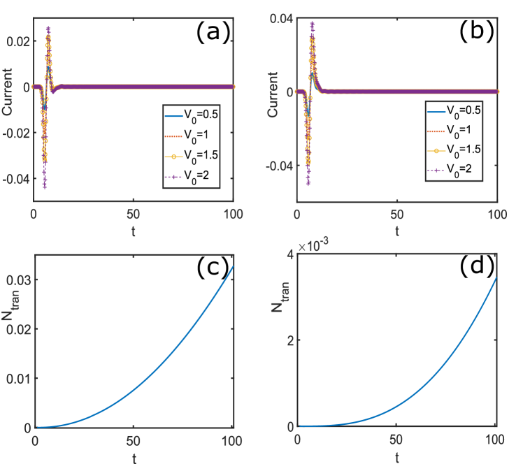
Figure 12: Ultrafast dynamics of RTM with the tight-binding dispersion relation, where $\Gamma=0.25$ and $\omega_{0}=1$. (a)-(b) The transient current for $\varepsilon_{d}=-0.5$ and $\varepsilon_{d}=0$; (c)-(d) The transport electron number $N_{\mathrm{tran}}$ for $\varepsilon_{d}=-0.5$ and $\varepsilon_{d}=0$.

References

- Basov et al. [2011] D. N. Basov, R. D. Averitt, D. Van Der Marel, M. Dressel, and K. Haule, Reviews of Modern Physics 83, 471 (2011).
- Kampfrath et al. [2013] T. Kampfrath, K. Tanaka, and K. A. Nelson, Nature Photonics 7, 680 (2013).
- Giannetti et al. [2016] C. Giannetti, M. Capone, D. Fausti, M. Fabrizio, F. Parmigiani, and D. Mihailovic, Advances in Physics 65, 58 (2016).
- Basov et al. [2017] D. N. Basov, R. D. Averitt, and D. Hsieh, Nature Materials 16, 1077 (2017).
- Cocker et al. [2013] T. L. Cocker, V. Jelic, M. Gupta, S. J. Molesky, J. A. J. Burgess, G. D. L. Reyes, L. V. Titova, Y. Y. Tsui, M. R. Freeman, and F. A. Hegmann, Nature Photonics 7, 620 (2013).
- Yoshioka et al. [2016] K. Yoshioka, I. Katayama, Y. Minami, M. Kitajima, S. Yoshida, H. Shigekawa, and J. Takeda, Nature Photonics 10, 762 (2016).
- Cocker et al. [2016] T. L. Cocker, D. Peller, P. Yu, J. Repp, and R. Huber, Nature 539, 263 (2016).
- Jelic et al. [2017] V. Jelic, K. Iwaszczuk, P. H. Nguyen, C. Rathje, G. J. Hornig, H. M. Sharum, J. R. Hoffman, M. R. Freeman, and F. A. Hegmann, Nature Physics 13, 591 (2017).
- Cuevas and Scheer [1990] J. C. Cuevas and E. Scheer, Molecular Electronics. An introduction to theory and experiment (World Scientific, 1990).
- Galperin et al. [2007] M. Galperin, M. a. Ratner, and A. Nitzan, Journal of Physics: Condensed Matter 19, 103201 (2007).
- Shi et al. [2018] T. Shi, E. Demler, and J. Ignacio Cirac, Annals of Physics 390, 245 (2018).
- Ashida et al. [2018a] Y. Ashida, T. Shi, M. C. Bañuls, J. I. Cirac, and E. Demler, Physical Review B 98, 024103 (2018a).
- Ashida et al. [2018b] Y. Ashida, T. Shi, M. C. Bañuls, J. I. Cirac, and E. Demler, Physical Review Letters 121, 26805 (2018b).
- Ng and Lee [1988] T. K. Ng and P. A. Lee, Phys. Rev. Lett. 61, 1768 (1988).
- Wingreen and Meir [1993] N. S. Wingreen and Y. Meir, Physical Review Letters 70, 2601 (1993).
- Wingreen and Meir [1994] N. S. Wingreen and Y. Meir, Physical Review B 49, 40 (1994).
- Ng [1996] T. K. Ng, Physical Review Letters 76, 487 (1996).
- Kaminski et al. [2000] A. Kaminski, Y. V. Nazarov, and L. I. Glazman, Phys. Rev. B. 62, 8154 (2000).
- Hewson and Meyer [2002] A. C. Hewson and D. Meyer, Journal of Physics Condensed Matter 14, 427 (2002).
- Legeza et al. [2008] O. Legeza, C. P. Moca, A. I. Toth, I. Weymann, and G. Zarand (2008), eprint arXiv:0809.3143.
- Holzner et al. [2010] A. Holzner, A. Weichselbaum, and J. Von Delft, Physical Review B - Condensed Matter and Materials Physics 81, 125126 (2010).
- Al-Hassanieh et al. [2006] K. A. Al-Hassanieh, A. E. Feiguin, J. A. Riera, C. A. Büsser, and E. Dagotto, Physical Review B 73, 195304 (2006).
- Heidrich-Meisner et al. [2009] F. Heidrich-Meisner, A. E. Feiguin, and E. Dagotto, Physical Review B 79, 235336 (2009).
- Eckel et al. [2010] J. Eckel, F. Heidrich-Meisner, S. G. Jakobs, M. Thorwart, M. Pletyukhov, and R. Egger, New Journal of Physics 12, 043042 (2010).
- Mahan [2000] G. Mahan, Many Particle Physics (Kluwer Academics/Plenum Publishers, 2000).
- Hewson [1993] A. C. Hewson, The Kondo Problem to Heavy Fermions-Cambridge University Press (1997) (Cambridge University Press, 1993).
- Kastner et al. [1998] M. a. Kastner, D. Goldhaber-Gordon, H. Shtrikman, D. Mahalu, D. Abusch-Magder, and U. Meirav, Nature 391, 156 (1998).
- S. M. Cronenwett et al. [1998] S. M. Cronenwett, T. H. Oosterkamp, and L. P. Kouwenhoven, Science 281, 540 (1998).
- Kouwenhoven and Glazman [2001] L. Kouwenhoven and L. Glazman, Physics World 14, 33 (2001).
- Bolech and Shah [2016] C. J. Bolech and N. Shah, Physical Review B 93, 085441 (2016).
- Stewart [1979] G. R. Stewart, Revews of Modern Physics 56, 755 (1979).
- Gegenwart et al. [2008] P. Gegenwart, Q. Si, and F. Steglich, Nature Physics 4, 186 (2008).
- Si and Steglich [2010] Q. Si and F. Steglich, Science 329, 1161 (2010).
- Kotliar and Vollhardt [2004] G. Kotliar and D. Vollhardt, Physics Today pp. 53–59 (2004).
- Andrei et al. [1983] N. Andrei, K. Furuya, and J. H. Lowenstein, Revews of Modern Physics 55, 331 (1983).
- Wiegmann and Tsvelik [1984] P. Wiegmann and A. M. Tsvelik, JETP Letters 83, 591 (1984).
- Bulla et al. [2008] R. Bulla, T. A. Costi, and T. Pruschke, Reviews of Modern Physics 80, 395 (2008).
- Read and Newns [1983] N. Read and D. M. Newns, Journal of Physics C: Solid State Physics 16, L1055 (1983).
- Kroha and Wolfle [1999] J. Kroha and P. Wolfle, Advances in Solid State Physics 39, 271 (1999).
- Georges et al. [1996] A. Georges, G. Kotliar, W. Krauth, and M. J. Rozenberg, Reviews of Modern Physics 68, 13 (1996).
- Feldbacher et al. [2004] M. Feldbacher, K. Held, and A. Assaad, Physical Review Letters 93, 136405 (2004).
- Rubtsov et al. [2005] A. N. Rubtsov, V. V. Savkin, and A. I. Lichtenstein, Physical Review B - Condensed Matter and Materials Physics 72, 035122 (2005).
- Werner et al. [2006] P. Werner, A. Comanac, L. De Medici, M. Troyer, and A. J. Millis, Physical Review Letters 97, 076405 (2006).
- Gull et al. [2011] E. Gull, A. J. Millis, A. I. Lichtenstein, A. N. Rubtsov, M. Troyer, and P. Werner, Reviews of Modern Physics 83, 349 (2011).
- Anders and Grewe [1994] F. B. Anders and N. Grewe, EPL (Europhysics Letters) 26, 551 (1994).
- Aoki et al. [2014] H. Aoki, N. Tsuji, M. Eckstein, M. Kollar, T. Oka, and P. Werner, Reviews of Modern Physics 86, 780 (2014).
- Cohen et al. [2013] G. Cohen, E. Gull, D. R. Reichman, A. J. Millis, and E. Rabani, Physical Review B 87, 195108 (2013).
- Kanász-Nagy et al. [2018] M. Kanász-Nagy, Y. Ashida, T. Shi, C. P. Moca, T. N. Ikeda, S. Fölling, J. I. Cirac, G. Zaránd, and E. A. Demler, Physical Review B 97, 155156 (2018).
- Kraus and Cirac [2010] C. V. Kraus and J. I. Cirac, New Journal of Physics 12, 113004 (2010).
- Cao et al. [2018] Y. Cao, D. G. Mazzone, D. Meyers, J. P. Hill, X. Liu, S. Wall, and M. P. M. Dean, Philosophiscal Transactions A arXiv:1809 (2018).
- Yang et al. [2007] D. S. Yang, N. Gedik, and A. H. Zewail, Journal of Physical Chemistry C 111, 4889 (2007).
- Stojchevska et al. [2010] L. Stojchevska, P. Kusar, T. Mertelj, V. V. Kabanov, X. Lin, G. H. Cao, Z. A. Xu, and D. Mihailovic, Physical Review B - Condensed Matter and Materials Physics 82, 1 (2010).
- Pomarico et al. [2017] E. Pomarico, M. Mitrano, H. Bromberger, M. A. Sentef, A. Al-Temimy, C. Coletti, A. Stöhr, S. Link, U. Starke, C. Cacho, et al., Physical Review B 95, 024304 (2017).
- Sch [2008] Science (New York, N.Y.) 321, 1649 (2008).
- Schmitt et al. [2011] F. Schmitt, P. S. Kirchmann, U. Bovensiepen, R. G. Moore, J. H. Chu, D. H. Lu, L. Rettig, M. Wolf, I. R. Fisher, and Z. X. Shen, New Journal of Physics 13 (2011).
- Gerber et al. [2017] S. Gerber, S. Yang, D. Zhu, H. Soifer, J. A. Sobota, S. Rebec, J. J. Lee, T. Jia, B. Moritz, C. Jia, et al., Science 75, 71 (2017).
- Nazarov [2003] Y. Nazarov, Quantum Noise in Mesoscopic Physics, NATO Science Series (Springer-Science+Business Media, B.v., 2003).
- Blanter and Buttiker [2000] Y. M. Blanter and M. Buttiker, Physics Reports 336, 1 (2000).
- Beenakker and Sch [2003] C. Beenakker and C. Sch, Physics Today p. 37 (2003).
- Kane and Fisher [1993] C. Kane and M. Fisher, Physical Review Letters 72, 724 (1993).
- Reznikov et al. [2002] M. Reznikov, V. Umansky, M. Heiblum, G. Bunin, R. De-Picciotto, and D. Mahalu, Physica B: Condensed Matter 249-251, 395 (2002).
- Sela et al. [2006] E. Sela, Y. Oreg, F. Von Oppen, and J. Koch, Physical Review Letters 97, 086601 (2006).
- Golub [2006] A. Golub, Physical Review B 73, 233310 (2006).
- Yamauchi et al. [2011] Y. Yamauchi, K. Sekiguchi, K. Chida, T. Arakawa, S. Nakamura, K. Kobayashi, T. Ono, T. Fujii, and R. Sakano, Physical Review Letters 106, 176601 (2011).
- Ament et al. [2011] L. J. P. Ament, M. van Veenendaal, T. P. Devereaux, J. P. Hill, and J. van den Brink, Reviews of Modern Physics 83, 705 (2011).
- Benjamin et al. [2013] D. Benjamin, D. Abanin, P. Abbamonte, and E. Demler, Physical Review Letters 110, 137002 (2013).
- Ganahl et al. [2015] M. Ganahl, M. Aichhorn, H. G. Evertz, P. Thunström, K. Held, and F. Verstraete, Physical Review B 92, 155132 (2015).