Synchronization of nonlinearly coupled networks of Chua oscillators

Abstract

The paper develops new sufficient conditions for synchronization of a network of $N$ nonlinearly coupled Chua oscillators interconnected via the first state coordinate only. The nonlinear coupling strength is governed by a function residing within a sector, i.e. it is bounded from above and below by linear functions. The derived sufficient conditions provide a trade-off between the characteristics of the sector and the interconnection topology of the network to guarantee the synchronization of the oscillators.

1 Introduction

Control and synchronization of nonlinear and chaotic systems have been intensively studied during the last decades (Pecora et al., 1997; Pecora and Carroll, 2015; Azar et al., 2017; Ochs et al., 2018; Raychowdhury et al., 2019). In particular, chaos synchronization has many potential applications in secure communication (Yang and Chua, 1997; Tse and Lau, 2003; Argyris et al., 2005), laser physics (Ohtsubo, 2002), chemical reactor process (Li et al., 2004), biomedical engineering (Strogatz, 2018). In this context, the Chua circuit appeared to be one of the most interesting objects for research since it exhibits extremely rich dynamical behavior and variety of bifurcation phenomena despite its structural simplicity. Investigation of synchronization abilities of coupled Chua oscillators may help to understand complex dynamical phenomena arising in networks of chaotic systems of more general types (Wu and Chua, 1994).

Synchronization of two linearly coupled Chua oscillators has been studied in Wu and Chua (1994); Wang and Liu (2006); Bowong and Tewa (2009); Wang et al. (1999); Zheng et al. (2002); Chen et al. (2010, 2012). In Wu and Chua (1994) it is conjectured that synchronization between two chaotic Chua circuits can be achieved by using the second state as the feedback variable for sufficiently large coupling constant. This conjecture has been analytically proven in Zheng et al. (2002) and Wang et al. (1999) utilizing Lyapunov-type arguments and a novel observer design methodology. Using the LaSalle invariance principle, a linear low-gain controller that exploits a single variable feedback (first state coordinate $x_{1}$) has been constructed in Chen et al. (2010). The robustness of this controller with respect to the perturbations of the parameters of Chua oscillators has been studied in Chen et al. (2012). Practical synchronization of chaotic systems with uncertainties via adaptive coupling mechanism has been investigated in Bowong and Tewa (2009). The synchronization of two identical chaotic and hyperchaotic systems with different initial conditions has been studied in Wang and Liu (2006).

A graph-spectral approach for the synchronization of a network of $N\in\mathbb{N}$ resistively coupled nonlinear oscillators has been proposed in Wu and Chua (1995). The sufficient conditions for synchronization have been derived from the connectivity graph, which describes how the oscillators are connected. An upper bound on the coupling conductance required for synchronization for arbitrary graphs has been obtained. Later, the synchronization of networks of $N\in\mathbb{N}$ nonlinear dynamical systems based on a state observer design approach has been studied in Jiang et al. (2006). Unlike the common diagonally coupling networks, see (Wang and Chen, 2003; Lü et al., 2004), where full state coupling is typically needed between two nodes, in Jiang et al. (2006) it is suggested that only a scalar coupling signal is required to achieve network synchronization. The presented approach has been applied to the chaos synchronization problem in two typical dynamical network configurations: global linear coupling and nearest-neighbor linear coupling, with each node being a modified Chua’s circuit. Finally, the problem of syhcnronizing an arbitrary subset of the nodes in the oscillatory network at fixed coupling stregth has been tackled in Gambuzza et al. (2019) by creation of appropriate network of additional interconnecting links between oscillators.

In the current paper, the sufficient conditions for the synchronization of the network of $N\in\mathbb{N}$ Chua oscillators interconnected with the static nonlinear coupling via the first state coordinate only are derived. These conditions provide a trade-off between characteristics of the connectivity graph and properties of the nonlinear coupling function to achieve synchronization.

The rest of the paper is organized as follows. In Section 2, the network under consideration is defined and the main problem of synchronization is formulated. In Section 3, the main result of the paper that is sufficient conditions for the synchronization of $N\in\mathbb{N}$ coupled Chua oscillators with static nonlinear coupling satisfying a so-called sector condition is derived. Also, numerical examples to illustrate the usage of the derived conditions are provided. In Section 4, a corollary of the main theorem for the case of two linearly coupled Chua oscillators is discussed and compared with the existing results in the literature. Finally, short conclusion and discussion in Section 5 complete the paper.

2 Problem Statement

Consider the extended Chua circuit system

$$\dot{x}_{1} =\alpha(-x_{1}+x_{2}-f(x_{1})){+u}, x_{1}(0)=x_{10}$$ (1a)

$$\dot{x}_{2} =x_{1}-x_{2}+x_{3}, x_{2}(0)=x_{20}$$ (1b)

$$\dot{x}_{3} =-\beta x_{2}-\gamma x_{3}, x_{3}(0)=x_{30}$$ (1c)

$$y =x_{1}$$ (1d)

with scalar piecewise linear function

$$f({x})=ax+\frac{1}{2}(b-a)(|x+1|-|x-1|)$$

and parameters $\alpha,\beta>0,\gamma\geq 0$, $a<b<0$. The system allows for vector-valued formulation

$$\dot{\bm{x}} =\bm{A}\bm{x}+{\bm{b}u}+\bm{f}(\bm{x}), \bm{x}(0)=\bm{x}_{0}$$ (2a)

$$y =\bm{c}^{T}\bm{x}$$ (2b)

with the state $\bm{x}{(t)}\in\mathbb{R}^{3}$, $\bm{x}_{0}^{T}=\begin{bmatrix}x_{10}&x_{20}&x_{30}\end{bmatrix}$, external input $u(t)\in\mathbb{R}$, which will be later used to interconnect Chua oscillators, and the matrix $\bm{A}$ and vectors $\bm{f},\bm{b},\bm{c}$ given by

$$\bm{A}=\begin{bmatrix}-\alpha&\alpha&0\\ 1&-1&1\\ 0&-\beta&-\gamma\end{bmatrix},\,\bm{f}(\bm{x})=\begin{bmatrix}-\alpha f(x_{1})\\ 0\\ 0\end{bmatrix},\,\bm{b}=\bm{c}=\begin{bmatrix}1\\ 0\\ 0\end{bmatrix}.$$

Now, consider a network of $N\in\mathbb{N}$ nodes described by a graph $\Gamma=(V,E)$ with vertex (node) set $V$ and edge set $E$, so that $|V|=N$. Let the associated adjacency matrix be given by $\bm{\mathcal{A}}=\{\alpha_{ij}\}_{i,j=1,\ldots,N}$, $\alpha_{ij}\in\left\{0,1\right\}$ with zero main diagonal.

Then, applying output feedback

$$u_{i}=-\sum_{j=1}^{N}\alpha_{ij}k(y_{i}-y_{j}),\quad i=1,\ldots,N$$

with an arbitrary nonlinear locally Lipschitz continuous coupling function $k:\mathbb{R}\to\mathbb{R}$, the dynamics of $N\in\mathbb{N}$ coupled Chua oscillators can be written as

$$\dot{\bm{x}}_{i} =\bm{A}\bm{x}_{i}-\bm{b}\sum_{j=1}^{N}\alpha_{ij}k(y_{i}-y_{j})+{\bm{f}(\bm{x_{i}})},\quad\bm{x}_{i}(0)=\bm{x}_{i0}$$ (3)

$$y_{i} =\bm{c}^{T}\bm{x}_{i},$$

for ${i}=1,\ldots,N$. For any given $\bm{\xi}\in\mathbb{R}^{3N}$ let $\bm{x}=(\bm{x}_{1},\ldots,\bm{x}_{N}):\mathbb{R}\to\mathbb{R}^{3N}$ denote a solution to (3) satisfying the initial condition $\bm{x}(0)=\bm{\xi}$. The Lipschitz continuity of the right-hand side of (3) guarantees the existence and uniqueness of the solution for any initial value $\bm{\xi}\in\mathbb{R}^{3N}$.

Associated to this network consider the relative synchronization errors with respect to the node 1

$$\bm{e}_{j}=\bm{x}_{j}-\bm{x}_{1},\quad{j}=1,\ldots,N.$$

The relative errors $\bm{e}_{ij}$ between arbitrary nodes $i$ and $j$ can be expressed using the relative errors $\bm{e}_{j}$ and $\bm{e}_{i}$

$$\bm{e}_{ij}=\bm{x}_{i}-\bm{x}_{j}=\bm{x}_{i}-\bm{x}_{1}-(\bm{x}_{j}-\bm{x}_{1})=\bm{e}_{i}-\bm{e}_{j}.$$

Accordingly, instead of analyzing $\frac{N(N-1)}{2}$ relative errors $\bm{e}_{ij}$ between connected nodes, it is sufficient to consider the behavior of the $N{-1}$ errors $\bm{e}_{j},\,{j=2},\ldots,N$.

The problem addressed in the sequel consists in providing sufficient conditions on the system parameters, the nonlinear coupling function $k$ and the network topology which ensure the synchronization of $N\in\mathbb{N}$ coupled Chua oscillators, i.e., the global convergence of the norms of errors $\bm{e}_{j}$ to zero:

$$\lim_{t\to\infty}\|\bm{e}_{j}(t)\|=0,\quad{j=2},\ldots,N.$$

3 Synchronization Conditions

Let $\{\bm{x}\}_{i}$ denote the $i$-th component of the vector $\bm{x}\in\mathbb{R}^{3}$, $i=1,2,3$. By splitting the state vector according to

$$\begin{bmatrix}z_{i}\\ \bm{\zeta}_{i}\end{bmatrix}=\begin{bmatrix}\{\bm{x}_{i}\}_{1}\\ \begin{bmatrix}\{\bm{x}_{i}\}_{2}\\ \{\bm{x}_{i}\}_{3}\end{bmatrix}\end{bmatrix},$$

rewrite the dynamics (3) in ${z}-\bm{\zeta}$ coordinates

$$\dot{z}_{i} =-\alpha z_{i}-\alpha f(z_{i})+\begin{bmatrix}\alpha&0\end{bmatrix}\bm{\zeta}_{i}$$ (4a)

$$\quad-\sum_{j=1}^{N}\alpha_{ij}k(z_{i}-{z_{j}})$$

$$\dot{\bm{\zeta}}_{i} =\begin{bmatrix}1\\ 0\end{bmatrix}z_{i}+\underbrace{\begin{bmatrix}-1&1\\ -\beta&-\gamma\end{bmatrix}}_{=:\bm{A}_{0}}\bm{\zeta}_{i},$$ (4b)

where matrix ${\bm{A}_{0}}$ is Hurwitz with eigenvalues $\lambda_{1,2}$ fulfilling $\mathfrak{R}(\lambda_{1,2})=-\mu_{0}<0$ with

$${-\mu_{0}=-\frac{1+\gamma}{2}+\mathfrak{R}\left(\sqrt{\frac{(1+\gamma)^{2}}{4}-(\gamma+\beta)}\right)},$$

where $\mathfrak{R}(\lambda)$ denotes the real part of $\lambda\in\mathbb{C}$.

Using the notation for the relative errors

$$\begin{bmatrix}e_{i}\\ \bm{\eta}_{i}\end{bmatrix}=\begin{bmatrix}z_{i}-z_{1}\\ \bm{\zeta}_{i}-\bm{\zeta}_{1}\end{bmatrix}$$

and taking into account that $e_{1}\equiv 0$, $\bm{\eta}_{1}\equiv\bm{0}$, the synchronization error dynamics can be written as

$$\dot{e}_{i} =-\alpha e_{i}-\alpha{\tilde{f}(e_{i})}+\begin{bmatrix}\alpha&0\end{bmatrix}\bm{\eta}_{i}$$ (5a)

$$\quad-\sum_{j=1}^{N}\Big{(}\alpha_{ij}k(e_{i}-e_{j})-\alpha_{1j}k(-e_{j})\Big{)}$$

$$\dot{\bm{\eta}}_{i} =\begin{bmatrix}1\\ 0\end{bmatrix}e_{i}+A_{0}\bm{\eta}_{i}$$ (5b)

with initial conditions $e_{i}(0)=e_{i,0}$ and $\bm{\eta}_{i}(0)=\bm{\eta}_{i,0}$, $i=2,\ldots,N$, and

$$\tilde{f}(e_{i})=f(z_{1}+e_{i})-f(z_{1}).$$ (6)

In the following subsection, sufficient conditions for global asymptotic stability of zero solution to the error dynamics system (5) will be derived. For this purpose additional sector requirement on the coupling function $k$ will be imposed.

3.1 Coupling with sector condition

Assumption 1

Coupling $k:\mathbb{R}\to\mathbb{R}$ is continuous odd function and there exist two constants $k_{2}\geq k_{1}\geq 0$ such that for all $e\in\mathbb{R}$:

$$k(e)e\geq 0,\quad k(-e)=-k(e),\quad k_{1}|e|\leq|k(e)|\leq k_{2}|e|.$$ (7)

Introduce the function

$$\tilde{k}(e)=k(e)-k_{2}e\quad\text{for all}\quad e\in\mathbb{R}.$$ (8)

From (7) and (8) it follows that functions $k$ and $\tilde{k}$ lie in the first-third and the second-fourth quadrant pairs respectively.

Lemma 2

Let Assumption 1 hold. Then

$$\left|\tilde{k}(e_{i}-e_{j})+\tilde{k}(e_{j})\right|\leq\left(k_{2}-k_{1}\right)|e_{i}|+\left(k_{2}-k_{1}\right)|e_{j}|$$ (9)

for all $e_{i},e_{j}\in\mathbb{R}$.

The left-hand side of (9) can be rewritten as

$$\begin{split}\left|\tilde{k}(e_{i}-e_{j})+\tilde{k}(e_{j})\right|&=|k(e_{i}-e_{j})-k_{2}(e_{i}-e_{j})\\ &\quad+k(e_{j})-k_{2}e_{j}|\\ &=\left|-k_{2}e_{i}+k(e_{j})-k(e_{j}-e_{i})\right|\end{split}$$

Consider the cases of positive and negative signs of the terms $e_{i},e_{j}$, and $e_{j}-e_{i}$ correspondingly. First, let $e_{i}\geq 0$, $e_{j}\geq 0$, $e_{j}-e_{i}\geq 0$. Then,

$$-k_{2}e_{i}+k_{1}e_{j}-k_{2}(e_{j}-e_{i}) \leq-k_{2}e_{i}+k(e_{j})-k(e_{j}-e_{i})$$

$$\leq-k_{2}e_{i}+k_{2}e_{j}-k_{1}(e_{j}-e_{i}),$$

which yields

$$|-k_{2}e_{i}+k(e_{j})-k(e_{j}-e_{i})|\leq(k_{2}-k_{1})|e_{j}|.$$ (10)

Let $e_{i}\geq 0$, $e_{j}\geq 0$, $e_{j}-e_{i}<0$. Then,

$$-k_{2}e_{i}+k_{1}e_{j}-k_{1}(e_{j}-e_{i}) \leq-k_{2}e_{i}+k(e_{j})-k(e_{j}-e_{i})$$

$$\leq-k_{2}e_{i}+k_{2}e_{j}-k_{2}(e_{j}-e_{i})$$

$$\leq 0,$$

which yields

$$|-k_{2}e_{i}+k(e_{j})-k(e_{j}-e_{i})|\leq(k_{2}-k_{1})|e_{i}|.$$ (11)

Let $e_{i}\geq 0$, $e_{j}<0$, $e_{j}-e_{i}<0$. Then,

$$-k_{2}e_{i}+k_{2}e_{j}-k_{1}(e_{j}-e_{i}) \leq-k_{2}e_{i}+k(e_{j})-k(e_{j}-e_{i})$$

$$\leq-k_{2}e_{i}+k_{1}e_{j}-k_{2}(e_{j}-e_{i})$$

which yields

$$|-k_{2}e_{i}+k(e_{j}) -k(e_{j}-e_{i})|$$ (12)

$$\leq(k_{2}-k_{1})|e_{i}|+(k_{2}-k_{1})|e_{j}|.$$

Similarly, one may check that for the rest combinations of the signs of $e_{i}$, $e_{j}$, and $e_{j}-e_{i}$ one of the inequalities (10), (11), (12) holds. Finally, combining (10), (11), (12), obtain that

$$\left|\tilde{k}(e_{i}-e_{j})+\tilde{k}(e_{j})\right|\leq\left(k_{2}-k_{1}\right)|e_{i}|+\left(k_{2}-k_{1}\right)|e_{j}|.$$

This completes the proof. $\square$

Denote the degree of node $i$ by $\kappa_{i}=\sum\limits_{j=1}^{N}\alpha_{ij}$ and rewrite the dynamics (5a) as follows:

$$\dot{e}_{i}= -\alpha e_{i}-\alpha\tilde{f}(e_{i})+\begin{bmatrix}\alpha&0\end{bmatrix}\bm{\eta}_{i}$$ (13)

$$-\sum_{j=1}^{N}\Big{(}\alpha_{ij}k(e_{i}-e_{j})+\alpha_{1j}k(e_{j})\Big{)}$$

$$= -\alpha e_{i}-\kappa_{i}k_{2}e_{i}-\alpha\tilde{f}(e_{i})+\begin{bmatrix}\alpha&0\end{bmatrix}\bm{\eta}_{i}$$

$$-\sum_{j=1}^{N}\Big{(}\alpha_{ij}\big{(}k(e_{i}-e_{j})-k_{2}(e_{i}-e_{j})\big{)}$$

$$+\alpha_{1j}k(e_{j})-\alpha_{ij}k_{2}e_{j}\Big{)}.$$

Introduce the residual connectivity coefficients with respect to the first node

$$\alpha_{1j} =\alpha_{ij}+\tilde{\alpha}_{ij},$$

$$\tilde{\alpha}_{ij} =\alpha_{1j}-\alpha_{ij}{=\begin{cases}0,&(i,j),(1,j)\in E,\\ 1,&(i,j)\notin E,(1,j)\in E,\\ -1,&(i,j)\in E,(1,j)\notin E,\\ 0,&(i,j),(1,j)\notin E,\end{cases}}$$

respectively. The expression inside the sum of (13) can be rewritten as

$$\alpha_{ij}\Big{(}k(e_{i} -e_{j})-k_{2}(e_{i}-e_{j})\Big{)}+\alpha_{1j}k(e_{j})-\alpha_{ij}k_{2}e_{j}$$

$$=\alpha_{ij}\Big{(}k(e_{i}-e_{j})-k_{2}(e_{i}-e_{j})\Big{)}$$

$$\quad+(\alpha_{ij}+\tilde{\alpha}_{ij})k(e_{j})-\alpha_{ij}k_{2}e_{j}$$

$$=\alpha_{ij}\Big{(}\tilde{k}(e_{i}-e_{j})+\tilde{k}(e_{j})\Big{)}+\tilde{\alpha}_{ij}k(e_{j}).$$

With these definitions the dynamics of $e_{i}$ can be written equivalently as

$$\dot{e}_{i}= -\alpha e_{i}-\kappa_{i}k_{2}e_{i}-\alpha\tilde{f}(e_{i})+\begin{bmatrix}\alpha&0\end{bmatrix}\bm{\eta}_{i}$$ (14)

$$-\sum_{j=1}^{N}\Big{(}\alpha_{ij}\big{(}\tilde{k}(e_{i}-e_{j})+\tilde{k}(e_{j})\big{)}+\tilde{\alpha}_{ij}k(e_{j})\Big{)}.$$

Following the reasoning in (Schaum, 2018) consider the implicit solution of the preceding ODEs (5b), (14) given by

$$e_{i}(t) =e^{-(\alpha+\kappa_{i}k_{2})t}e_{i,0}$$ (15)

$$+ \int_{0}^{t}e^{-(\alpha+\kappa_{i}k_{2})(t-\tau)}\bigg{(}-\alpha\tilde{f}(e_{i}(\tau))+\begin{bmatrix}\alpha&0\end{bmatrix}\bm{\eta}_{i}(\tau)$$

$${-} \sum_{j=1}^{N}\left(\alpha_{ij}\left(\tilde{k}(e_{i}-e_{j})+\tilde{k}(e_{j})\right)+\tilde{\alpha}_{ij}k(e_{j})\right)\bigg{)}d\tau$$

$$\bm{\eta}_{i}(t) =e^{\bm{A}_{0}t}\bm{\eta}_{i,0}+\int_{0}^{t}e^{\bm{A}_{0}(t-\tau)}\begin{bmatrix}1\\ 0\end{bmatrix}e_{i}(\tau)d\tau.$$

Since function $f$ is Lipschitz continuous with Lipschitz constant $|a|$ it holds that

$$|\tilde{f}(e_{i})|=|f(z_{1}+e_{i})-f(z_{1})|\leq|a||e_{i}|$$ (16)

for any $e_{i}\in\mathbb{R}$. Taking norms on both sides of (15), applying the triangle inequality, and accounting for Lemma 2 and inequality (16) the estimates

$$|e_{i}(t)| \leq e^{-(\alpha+\kappa_{i}k_{2})t}$$

$$\times\left(|e_{i,0}|+\int_{0}^{t}{e^{(\alpha+\kappa_{i}k_{2})\tau}}\Bigl{(}\alpha|a||e_{i}(\tau)|+\alpha\|\bm{\eta}_{i}(\tau)\|\right.$$

$$\left.{+}\sum_{j=1}^{N}\left(\alpha_{ij}(\left(k_{2}-k_{1}\right)|e_{i}(\tau)|+\left(k_{2}-k_{1}\right)|e_{j}(\tau)|)\right.\right.$$

$$\left.\left.{+}|\tilde{\alpha}_{ij}|k_{2}|e_{j}(\tau)|\right)\Bigr{)}d\tau\right)$$

$$\|\bm{\eta}_{i}(t)\| \leq e^{-\mu_{0}t}\left(\|\bm{\eta}_{i,0}\|+\int_{0}^{t}{e^{\mu_{0}\tau}}|e_{i}(\tau)|d\tau\right)$$

hold. Define the right-hand sides of the preceding inequalities as $\sigma_{i}$ and $\chi_{i}$, i.e.,

$$\begin{split}\sigma_{i}&=e^{-(\alpha+\kappa_{i}k_{2})t}\\ &\times\left(|e_{i,0}|+\int_{0}^{t}{e^{(\alpha+\kappa_{i}k_{2})\tau}}\Big{(}\alpha|a||e_{i}(\tau)|+\alpha\|\bm{\eta}_{i}(\tau)\|\right.\\ &\left.{+}\sum_{j=1}^{N}\left(\alpha_{ij}(\left(k_{2}-k_{1}\right)|e_{i}(\tau)|+\left(k_{2}-k_{1}\right)|e_{j}(\tau)|)\right.\right.\\ &\left.\left.+|\tilde{\alpha}_{ij}|k_{2}|e_{j}(\tau)|\right)\Big{)}d\tau\right)\end{split}$$

$$\chi_{i} =e^{-\mu_{0}t}\left(\|\bm{\eta}_{i,0}\|+\int_{0}^{t}{e^{\mu_{0}\tau}}|e_{i}(\tau)|d\tau\right)$$

so that $|e_{i}(t)|\leq\sigma_{i}(t)$ and $\|\bm{\eta}_{i}(t)\|\leq\chi_{i}(t)$ for all $t\geq 0$ with $|e_{i}(0)|=\sigma_{i}(0)$ and $\|\bm{\eta}_{i}(0)\|=\chi_{i}(0)$ for all $i=2,\ldots,N$. Since $e_{1}(t)=0$ for all $t\geq 0$, let $\sigma_{1}(t)\equiv 0$ so that $|e_{i}(t)|\leq\sigma_{i}(t)$ holds for all $i=1,\ldots,N$. The time derivatives of $\sigma_{i}$ and $\chi_{i}$ can be estimated by

$$\begin{split}\dot{\sigma}_{i}(t)=&-(\alpha+\kappa_{i}k_{2})\sigma_{i}(t)+\alpha|a||e_{i}(t)|+\alpha\|\bm{\eta}_{i}(t)\|\\ &+\sum_{j=1}^{N}\big{(}\alpha_{ij}\left(\left(k_{2}-k_{1}\right)|e_{i}|+\left(k_{2}-k_{1}\right)|e_{j}|\right)\\ &+|\tilde{\alpha}_{ij}|k_{2}|e_{j}(t)|\big{)}\\ \leq&-(\alpha-\alpha|a|+\kappa_{i}k_{1})\sigma_{i}(t)+\alpha\chi_{i}(t)\\ &+\sum_{j=1}^{N}\left(|\alpha_{ij}|(k_{2}-k_{1})+|\tilde{\alpha}_{ij}|k_{2}\right)\sigma_{j}(t)\end{split}$$

$$\begin{split}\dot{\chi}_{i}(t)=&-\mu_{0}\chi_{i}(t)+|e_{i}(t)|\\ \leq&-\mu_{0}\chi_{i}(t)+\sigma_{i}(t).\end{split}$$

Taking into account that $\sigma_{1}(t)\equiv 0$, the preceding dynamics can be written in vector notation as

$$\frac{d}{dt}\begin{bmatrix}\sigma_{i}\\ \chi_{i}\end{bmatrix} \leq\begin{bmatrix}-(\alpha-\alpha|a|+\kappa_{i}k_{1})&\alpha\\ 1&-\mu_{0}\end{bmatrix}\begin{bmatrix}\sigma_{i}\\ \chi_{i}\end{bmatrix}$$ (17)

$$+\begin{bmatrix}\sum_{j=2}^{N}\left(|\alpha_{ij}|(k_{2}-k_{1})+|\tilde{\alpha}_{ij}|k_{2}\right)\sigma_{j}\\ 0\end{bmatrix}.$$

Introducing $\bm{z}=\begin{bmatrix}\sigma_{2}&\cdots&\sigma_{N}&\chi_{2}&\cdots&\chi_{N}\end{bmatrix}^{T}$, inequality (17) can be written as

$$\dot{\bm{z}} \leq\underbrace{\begin{bmatrix}-(\alpha-\alpha|a|)\mathbf{I}-k_{1}\mathbf{K}+(k_{2}-k_{1})\bm{\mathcal{A}}_{1}+k_{2}\bm{\mathcal{A}}_{2}&\alpha\mathbf{I}\\ \mathbf{I}&-\mu_{0}\mathbf{I}\end{bmatrix}}_{=:\mathbf{M}}\bm{z}$$ (18)

with matrices

$$\bm{\mathcal{A}}_{1} =\begin{bmatrix}0&|\alpha_{23}|&\cdots&|\alpha_{2N}|\\ |\alpha_{32}|&0&\ddots&\vdots\\ \vdots&\ddots&\ddots&\vdots\\ |\alpha_{N2}|&\cdots&\cdots&0\end{bmatrix},$$

$$\bm{\mathcal{A}}_{2} =\begin{bmatrix}0&|\alpha_{23}-\alpha_{13}|&\cdots&|\alpha_{2N}-\alpha_{1N}|\\ |\alpha_{32}-\alpha_{12}|&0&\ddots&\vdots\\ \vdots&\ddots&\ddots&\vdots\\ |\alpha_{N2}-\alpha_{12}|&\cdots&\cdots&0\end{bmatrix},$$

$\mathbf{K}=\text{diag}\{\kappa_{2},\ldots,\kappa_{N}\}$, and $(N-1)\times(N-1)$–dimensional identity matrix $\mathbf{I}$. Sufficient conditions for the synchronization of the entire network can be formulated in terms of the eigenvalues of the matrix $\mathbf{M}$.

Theorem 3

Let Assumtion 1 hold and matrix $\mathbf{M}$ defined in (18) be Hurwitz. Then, the norm of errors between the states of Chua oscillators (3) converges exponentially to zero.

The differential inequality (17) for $\sigma_{i}$ contains both stabilizing and destabilizing terms, which have physical interpretation and can be used as guidelines for the coupling design. In particular, the stabilizing term becomes larger with the growth of the lower bound $k_{1}$ of the nonlinear coupling. The destabilizing terms vanish when the lower bound $k_{1}$ approaches the upper bound $k_{2}$ and the interconnection graph is fully connected (i.e. the coefficients $\tilde{\alpha}_{ij}$ are zero). These effects can be reached by choosing the coupling $k$ with a sufficiently large lower bound $k_{1}$.

3.2 Numerical example

3.2.1 Example 1.

Consider a fully connected network of $N=20$ Chua oscillators (3) with parameters $\alpha=15.61$, $\beta=25.581$, $\gamma=0$, $a=-1.142$, $b=-0.715$, and nonlinear coupling

$$k(e)=3e+\arctan{(e)}\quad\text{for all}\quad e\in\mathbb{R}.$$ (19)

The chosen parameters correspond to the chaotic behavior of each oscillator (Pivka et al., 1994). Oscillators’ trajectories converge to an attractor that has a double scroll shape in three dimensional state space (see Fig. 1).

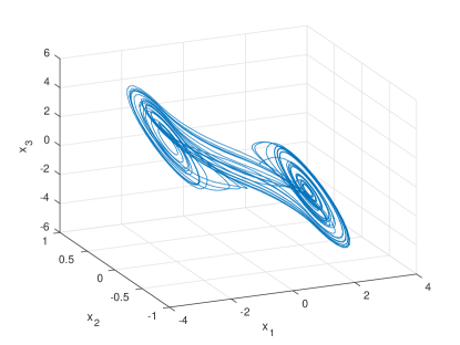
Figure 1: Double scroll attractor for the coupled chaotic Chua oscillators from Example 1.

Nonlinear coupling strength (19) satisfies the sector condition (7) with constants $k_{1}=3$ and $k_{2}=4$. For the chosen parameters and the interconnection coupling (19) the matrix $\mathbf{M}$ defined in (18) reads

$$\mathbf{M}=\begin{bmatrix}-54.7834\mathbf{I}&15.61\mathbf{I}\\ \mathbf{I}&-0.5\mathbf{I}\end{bmatrix}+\begin{bmatrix}\mathbf{1}{\mathbf{1}}^{\top}-\mathbf{I}&\mathbf{0}\\ \mathbf{0}&\mathbf{0}\end{bmatrix},$$

where $\mathbf{0}$ denotes zero $(N-1)\times(N-1)$–matrix, and $\mathbf{1}$ denotes $(N-1)$–dimensional vector $\begin{bmatrix}1&1&\cdots&1\end{bmatrix}^{\top}$. By direct calculation one may check that all eigenvalues lie in the open left half-plane

$$\mathfrak{R}(\lambda(\mathbf{M}))\in[-56.0643,-0.0748].$$

Hence, from Theorem 3 it follows that the oscillators are synchronized. The state evolution for $N=20$ oscillators is shown in Fig. 2.

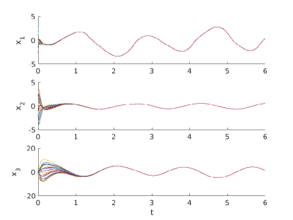
Figure 2: Time evolution of $N=20$ coupled chaotic Chua oscillators with interconnection coupling (19).

4 Synchronization of two oscillators

In this section a corollary from Theorem 3 for the case of two Chua oscillators connected with linear coupling

$$k(e)=ke\quad\text{for all}\quad e\in\mathbb{R}$$ (20)

with coupling constant $k>0$ is presented. Obviously, the function (20) satisfies the sector condition (7) with $k_{1}=k_{2}=k$.

Corollary 4

In the case of two Chua oscillators (3) connected via the first state variable with linear coupling (20) the condition for synchronization reads

$$k>\alpha\left(|a|+\frac{1}{\mu_{0}}-1\right),$$ (21)

i.e., the synchronization emerges if the coupling between the first state of each oscillator is sufficiently strong.

For the case of two Chua oscillators the matrix $\mathbf{M}$ from (18) is a $2\times 2$–matrix defined by

$$\mathbf{M}=\begin{bmatrix}-(\alpha-\alpha|a|+k)&\alpha\\ 1&-\mu_{0}\end{bmatrix}.$$

Due to the Routh-Hurwitz criterion, the roots of the corresponding characteristic polynomial

$$\lambda^{2}+\lambda\left(\mu_{0}+\alpha-\alpha|a|+k\right)+\left(\alpha-\alpha|a|+k\right)\mu_{0}-\alpha=0$$

are in the open left half-plane if and only if

$$\begin{cases}\mu_{0}+\alpha-\alpha|a|+k>0,\\ \left(\alpha-\alpha|a|+k\right)\mu_{0}-\alpha>0,\end{cases}$$

which yields

$$k>\alpha\left(|a|+\frac{1}{\mu_{0}}-1\right).$$

This completes the proof. $\square$

The problem of the synchronization of two identical Chua oscillators via the first state variable by linear coupling addressed in Corollary 4 has been also successfully tackled in Chen et al. (2010, 2012) for the case of $\gamma=0$ by employing the Lyapunov method. The constraint on the coupling constant obtained in Chen et al. (2010, 2012) reads as

$$k>\alpha|a|,$$

which is less a conservative condition compared to (21). However, the applicability of Theorem 3 is more general even in the case of two oscillators due to the possibility of $\gamma\not=0$. Besides this, the approach proposed in the present paper handles the case of an arbitrary number of Chua oscillators with an arbitrary interconnection topology and nonlinear coupling functions.

4.0.1 Example 2.

Consider two Chua oscillators with parameters $\alpha=10$, $\beta=15$, $\gamma=0.1$, $a=-1.31$, $b=-0.75$, which are linearly coupled via the first state coordinate. By direct calculation we obtain that

$$-\mu_{0}=-\frac{1.1}{2}+\mathfrak{R}\left(\sqrt{\frac{1.21}{4}-15}\right)=-\frac{1.1}{2}.$$

From Corollary 4, the coupling constant $k$ should be chosen larger than

$$k>10\left(1.31+\frac{2}{1.1}-1\right)\approx 21.282.$$

The state evolution of both oscillators for $k=21.3$ is shown in Fig. 3.

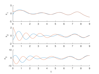
Figure 3: Time evolution of two coupled chaotic Chua oscillators with interconnection gain $k=21.3$.

5 Conclusion and Outlook

The synchronization of a network of $N\in\mathbb{N}$ Chua oscillators which are coupled via the first state coordinate with static nonlinear coupling is studied. Sufficient conditions for the synchronization are formulated in terms of the eigenvalues of the auxiliary matrix $\mathbf{M}$, whose entries represent the interplay between the parameters of the oscillators, the interconnection topology of the network and the characteristics of the nonlinear coupling function.

The extension of the derived conditions to the class of dynamically coupled Chua oscillators will allow for analysis of wide classes of memristive networks and, more generally, time-varying interconnections which are capable to model the bio-inspired plasticity phenomenon. Another interesting research direction is the study of multi-clustering capabilities of oscillatory networks and control design approaches for this kind of behaviour.

References

- Argyris et al. (2005) Argyris, A., Syvridis, D., Larger, L., Annovazzi-Lodi, V., Colet, P., Fischer, I., Garcia-Ojalvo, J., Mirasso, C.R., Pesquera, L., and Shore, K.A. (2005). Chaos-based communications at high bit rates using commercial fibre-optic links. Nature, 438(7066), 343.
- Azar et al. (2017) Azar, A.T., Vaidyanathan, S., and Ouannas, A. (2017). Fractional order control and synchronization of chaotic systems, volume 688. Springer.
- Bowong and Tewa (2009) Bowong, S. and Tewa, J.J. (2009). Practical adaptive synchronization of a class of uncertain chaotic systems. Nonlinear Dynamics, 56(1-2), 57.
- Chen et al. (2012) Chen, F., Ji, G., Zhai, S., Wang, S., Zhou, S., and Zhang, T. (2012). Uncertain Chua system chaos synchronization using single variable feedback based on adaptive technique. In Proceedings of the 2012 IEEE International Conference on Information and Automation (ICIA-2012), 196–199.
- Chen et al. (2010) Chen, F., Zhang, C., Ji, G., Zhai, S., and Zhou, S. (2010). Chua system chaos synchronization using single variable feedback based on LaSalle invariance principal. In Proceedings of the 2010 IEEE International Conference on Information and Automation (ICIA-2010), 301–304.
- Gambuzza et al. (2019) Gambuzza, L.V., Frasca, M., and Latora, V. (2019). Distributed control of synchronization of a group of network nodes. IEEE Transactions on Automatic Control, 64(1), 365–372.
- Jiang et al. (2006) Jiang, G.P., Tang, W.K.S., and Chen, G. (2006). A state-observer-based approach for synchronization in complex dynamical networks. IEEE Transactions on Circuits and Systems I: Regular Papers, 53 (12), 2739–2745.
- Li et al. (2004) Li, Y.N., Chen, L., Cai, Z.S., and Zhao, X.Z. (2004). Experimental study of chaos synchronization in the Belousov–Zhabotinsky chemical system. Chaos, Solitons & Fractals, 22(4), 767–771.
- Lü et al. (2004) Lü, J., Yu, X., and Chen, G. (2004). Chaos synchronization of general complex dynamical networks. Physica A: Statistical Mechanics and its Applications, 334(1-2), 281–302.
- Ochs et al. (2018) Ochs, K., Michaelis, D., and Roggendorf, J. (2018). Generalized Kuramoto Model: Circuit Synthesis and Electrical Interpretation of Synchronization. submitted to International Symposium on Circuits and Systems 2019.
- Ohtsubo (2002) Ohtsubo, J. (2002). Chaos synchronization and chaotic signal masking in semiconductor lasers with optical feedback. IEEE Journal of Quantum Electronics, 38(9), 1141–1154.
- Pecora and Carroll (2015) Pecora, L.M. and Carroll, T.L. (2015). Synchronization of chaotic systems. Chaos: An Interdisciplinary Journal of Nonlinear Science, 25(9), 097611.
- Pecora et al. (1997) Pecora, L.M., Carroll, T.L., Johnson, G.A., Mar, D.J., and Heagy, J.F. (1997). Fundamentals of synchronization in chaotic systems, concepts, and applications. Chaos: An Interdisciplinary Journal of Nonlinear Science, 7(4), 520–543.
- Pivka et al. (1994) Pivka, L., Wu, C.W., and Huang, A. (1994). Chua’s oscillator: A compendium of chaotic phenomena. Journal of Franklin Institute, 331 (6), 705–741.
- Raychowdhury et al. (2019) Raychowdhury, A., Parihar, A., Smith, G.H., Narayanan, V., Csaba, G., Jerry, M., Porod, W., and Datta, S. (2019). Computing with networks of oscillatory dynamical systems. Proceedings of the IEEE, 107(1), 73–89.
- Schaum (2018) Schaum, A. (2018). Strong detectability and unknown input observer design for a class of networks of systems. IFAC-PapersOnLine, 51(23), 46 – 51. 7th IFAC Workshop on Distributed Estimation and Control in Networked Systems NECSYS 2018.
- Strogatz (2018) Strogatz, S.H. (2018). Nonlinear dynamics and chaos: with applications to physics, biology, chemistry, and engineering. CRC Press.
- Tse and Lau (2003) Tse, C. and Lau, F. (2003). Chaos-based digital communication systems. Operating Principles, Analysis Methods and Performance Evaluation (Springer Verlag, Berlin, 2004).
- Wang and Liu (2006) Wang, F. and Liu, C. (2006). A new criterion for chaos and hyperchaos synchronization using linear feedback control. Physics Letters A, 360(2), 274–278.
- Wang and Chen (2003) Wang, X.F. and Chen, G. (2003). Complex networks: small-world, scale-free and beyond. IEEE Circuits and Systems Magazine, 3(1), 6–20.
- Wang et al. (1999) Wang, X.F., Wang, Z.Q., and Chen, G. (1999). A new criterion for synchronization of coupled chaotic oscillators with application to Chua’s circuits. International Journal of Bifurcation and Chaos, 9(06), 1169–1174.
- Wu and Chua (1995) Wu, C.W. and Chua, L.O. (1995). Application of graph theory to the synchronization in an array of coupled nonlinear oscillators. IEEE Transactions on Circuits and Systems I: Fundamental Theory and Applications, 42 (8), 494–497.
- Wu and Chua (1994) Wu, C.W. and Chua, L.O. (1994). A unified framework for synchronization and control of dynamical systems. International Journal of Bifurcation and Chaos, 4(04), 979–998.
- Yang and Chua (1997) Yang, T. and Chua, L.O. (1997). Impulsive stabilization for control and synchronization of chaotic systems: theory and application to secure communication. IEEE Transactions on Circuits and Systems I: Fundamental Theory and Applications, 44(10), 976–988.
- Zheng et al. (2002) Zheng, Y., Liu, Z., and Zhou, J. (2002). A new synchronization principle and application to Chua’s circuits. International Journal of Bifurcation and Chaos, 12 (4), 815.