Geodesic nets: some examples and open problems

Abstract.

Geodesic nets on Riemannian manifolds form a natural class of stationary objects generalizing geodesics. Yet almost nothing is known about their classification or general properties even when the ambient Riemannian manifold is the Euclidean plane or the round $2$-sphere.

In the first half of this paper we survey some results and open questions (old and new) about geodesic nets on Riemannian manifolds. Many of these open questions are about geodesic nets on the Euclidean plane. The second half contains a partial answer for one of these questions, namely, a description of a new infinite family of geodesic nets on the Euclidean plane with 14 boundary (or unbalanced) vertices and arbitrarily many inner (or balanced) vertices of degree $\geq 3$.

1. Overview

1.1. Geodesic nets and multinets: definition

Let $M$ be a Riemannian manifold, $S$ a finite (possibly empty) set of points in $M$, and $G$ a finite multigraph (or, more formally, a finite $1$-dimensional cell complex). A geodesic net modelled on $G$ with vertices $S$ is a smooth embedding $f$ of $G$ into $M$ such that:

1. Every point from $S$ is the image under $f$ of a vertex of $G$;

2. For each $1$-parametric flow $\Phi_{t},\ t\in(-\epsilon,\epsilon),$ of diffeomorphisms of $M$ fixing all points of $S$ with $\Phi_{0}=Id$, $t=0$ is the critical point of the function $l(t)$ defined as the length of $\Phi_{t}(f(G))$.

Less formally, geodesic nets on $M$ are critical points (not necessarily local minima!) of the length functional on the space of embedded multigraphs into $M$, where a certain subset of the set of vertices must be mapped to prescribed points of $M$.

The simplest example of geodesic nets arises when $S$ is a set of two points $x,y$, and $G=[0,1]$ the graph with two vertices and one edge. In this case, the geodesic nets modelled on $G$ with vertices $x,y$ are precisely non-self-intersecting geodesics in $M$ connecting $x$ and $y$. Self-intersecting geodesics can be modelled on more complicated graphs, but if we wish to model them on the same $G$ it makes sense to modify our definition of geodesic nets by allowing $f$ to be only an immersion on the union of interiors of edges. In other words, one may allow edges to self-intersect and to intersect each other. In particular, we are allowing that two different edges between the same pair of vertices might have the same image. As the result, the images of edges of $G$ in $M$ acquire multiplicities that can be arbitrary positive integer numbers. In this paper we are going to call geodesic nets defined using immersions rather than embeddings of multigraphs geodesic multinets.

Applying the first variation formula for for the length functional we see that the above definition of a geodesic (multi)net is equivalent to the following:

Definition 1.1.1.

Let $S$ be a (possibly empty) finite set of points in a Riemannian manifold $M$. A geodesic net on $M$ consists of a finite set $V$ of points of $M$ (called vertices) that includes $S$ and a finite set $E$ of non-constant distinct geodesics between vertices (called edges) so that for every vertex $v\in V\setminus S$ the following balancing condition holds: Consider the unit tangent vectors at $v$ to all edges incident to $v$. Direct each tangent vector from $v$ towards the other endpoint of the edge. Then the sum of all these tangent vectors must be equal to $0\in T_{v}M$. Further, edges are not allowed to intersect or self-intersect. Geodesic multinets are defined in the same way with the two following distinctions: 1) Edges are allowed to intersect and self-intersect; 2) Each edge is endowed with a positive integer multiplicity; the tangent vector to an edge enters the sum in the balancing condition at each its endpoint with the multiplicity equal to the multiplicity of the corresponding edge.

Vertices in $S$ are called boundary or unbalanced, vertices in $V\setminus S$ are called inner, or free, or balanced (as the balancing condition must hold only at each vertex in $V\setminus S$). If $v$ is an unbalanced vertex, then the sum of all unit tangent vectors to edges incident to $v$ need not be equal to the zero vector. We call this sum the imbalance vector $\operatorname{Imb}(v)$ at $v$, and its norm the imbalance, $\operatorname{imb}(v)$, at $v$. The sum of imbalances $\sum_{v\in S}\operatorname{imb}(v)$ over the set of all unbalanced points is called the total imbalance of the geodesic net. It is convenient to define $\operatorname{Imb}(v)$ also at balanced vertices as zero vectors in $T_{v}M$.

For the rest of the paper we are going to require that no balanced vertex is isolated, that is, has degree zero. As the degree of a balanced vertex clearly cannot be one, we see that the minimal degree of a balanced vertex becomes two. The balancing condition implies that for any balanced vertex of degree $2$, its two incident edges can be merged into a single geodesic. Conversely, we can subdivide each edge of a geodesic net by inserting as many new balanced vertices of degree $2$ as we wish. As now the role of balanced vertices of degree $2$ in the classification of geodesic nets is completely clear, we are going to consider below only geodesic nets where all balanced vertices have degree $\geq 3$. It is clear that we can add or remove geodesics connecting unbalanced vertices at will without affecting the balancing condition at a balanced vertex. Therefore, we agree that all considered geodesic nets do not contain edges between unbalanced vertices. Our final convention is that we are going to consider here only connected geodesic (multi)nets (as the classification of disconnected nets obviously reduces to classification of their connected components).

1.2. Geodesic nets in Euclidean spaces.

A significant part of this paper will be devoted to geodesic nets in Euclidean spaces, in particular, in the Euclidean plane. In this case above definition says that a geodesic multinet is a graph $G=(V,E)$ in $\mathbb{R}^{n}$ such that 1) $S$ is a subset of the set of vertices $V$, 2) each edge is a straight line segment between its endpoints, and is endowed with a positive integer multiplicity $n(e)$, 3) For each vertex $v\in V\setminus S$, there is zero imbalance, i.e. $\sum_{e\in I(v)}n(e)\frac{e}{\|e\|}=0$, where $I(v)$ denotes the set of edges incident to $v$, and $e$ denotes an edge regarded as the vector in $\mathbb{R}^{n}$ directed from $v$ towards the other endpoint. For geodesic nets, all $n(e)$ must be equal to $1$, and, in addition, different edges are not allowed to intersect. Figure 1.2.1 depicts examples of balanced points of degrees $3$, $4$ and $7$ in $\mathbb{R}^{2}$. It is easy to see that 1) the angles between edges incident to a balanced vertex of degree $3$ are always equal to $120$ degrees. (This will be true not only for $\mathbb{R}^{2}$ but for all ambient Riemannian manifolds $M$.) 2) A balanced vertex $v$ of degree $4$ in the Euclidean plane is a point of intersection of two straight line segments formed by two pairs of incident edges at $v$ (see Figure 1.2.1).

Figure 1.2.1. Examples for balanced vertices of degree $3$, $4$ and $7$.

Here are some other easily verified facts about geodesic (multi)nets in Euclidean spaces:

1. Each geodesic multinet is contained in the convex hull of its unbalanced vertices.

2. As a corollary each geodesic (multi)net with two boundary vertices is simply the straight line segment connecting these points (that can be endowed with any positive integer multiplicity in the case of geodesic multinets).

Therefore, the interesting part of the classification of geodesic (multi)nets in the Euclidean plane starts from the case of three boundary points.

1. For each geodesic (multi)net in $\mathbb{R}^{n}$ we can consider $\operatorname{Imb}(v)$ as vectors in the ambient space $\mathbb{R}^{n}$. Therefore, in this case one can also define the total imbalance vector. Yet this vector is always zero:

   $$\sum_{v\in S}\operatorname{Imb}(v)=\sum_{v\in V}\operatorname{Imb}(v)=0,\ \ \ (1.2.1)$$

   Indeed, the second sum can be represented as the sum of contributions of individual edges. Each edge contributes two oppositely directed vectors that enter sums in the definition of imbalance vectors at its endpoints. Therefore, the sum over edges of edge contributions is zero.

2. For a geodesic (multi)net $N$ in a Euclidean space its length $L(N)$ is given by the following formula:

   $$L(N)=-\sum_{v\in S}\langle v,\operatorname{Imb}(v)\rangle.\ \ \ (1.2.2)$$

   In the right hand side we perform the summation over the set of all unbalanced vertices; each vertex is also regarded as a vector in $\mathbb{R}^{n}$.
   Proof: In order to prove this formula, first observe that the right hand side does not change when we change the origin of the coordinate system in $\mathbb{R}^{n}$. (This easily follows from the formula (1.2.1).) Therefore, we can assume that the origin is not on the net. For each positive $r$ let $D_{r}$ denote the ball of radius $r$ centered at the origin, $\partial D_{r}$ its boundary, $E(r)$ the set of edges of the net intersecting $\partial D_{r}$. For each $e\in E(r)$ let $e(r)$ denote the point of intersection of $e$ and $\partial D_{r}$. Formula (1.2.2) is an immediate corollary of the following formula, when it is applied to very large values of $r$:

   $$L(N\bigcap D_{r})=\sum_{e\in E(r)}\langle e(r),\frac{e}{\|e\|}\rangle-\sum_{v\in D_{r}}\langle v,\operatorname{Imb}(v)\rangle.\ \ \ (1.2.3)$$

   In this formula we regard $e$ also as a vector in $\mathbb{R}^{n}$. We choose its direction from $e(r)$ towards the interior of $D_{r}$. This formula obviously holds, when $r$ is small, as both sides are equal to zero. Define special values of $r$ as those, where $\partial D_{r}$ is either tangent to one of the edges or passes through one of the vertices. There are only finitely many special values of $r$. Our next observation which is easy to verify is that the right hand side of (1.2.3) changes continuously, when $r$ passes through its special value. (Obviously, one needs only to check what happens if $\partial D_{r}$ passes through a balanced or an unbalanced vertex.) Now we see that it is sufficient to check that the derivatives of the right hand side and the left hand side with respect to $r$ at each non-special point coincide. Each of these derivatives will be a sum over edges in $E(r)$. To complete the proof it is sufficient to verify that the contributions of each edge to both sides are the same. Each such edge $e$ contributes $\frac{1}{\cos\theta_{e}(r)}$ to the derivative of the left hand side, where $\theta_{e}(r)$ denotes the angle between $e$ and $e(r)$. Its contribution to the right hand side is $(r\cos\theta_{e}(r))^{\prime}=\cos\theta_{e}(r)-r\sin\theta_{e}(r)\frac{d\theta_{e}(r)}{dr}=\frac{1}{\cos\theta_{e}(r)},$ as an easy trigonometric argument implies that $\frac{d\theta_{e}(r)}{dr}=-\frac{\tan\theta_{e}(r)}{r}.$ This completes the proof of (1.2.3) and, therefore (1.2.2).

1.3. Steiner trees and locally minimal geodesic nets.

Figure 1.3.1. A geodesic net with $3$ unbalanced vertices and $1$ balanced vertex (the Fermat Point). This is in fact the maximal number of balanced vertices when only given $3$ unbalanced vertices on the plane with a metric of nonpositive curvature. On the other hand, the two Steiner trees for four points are not maximal regarding the number of balanced vertices of a geodesic net with four unbalanced vertices.

Study of geodesic nets was originally motivated by the following question posed by Gauß: Given a set of points on the plane, connect them by means of a graph of the minimal possible length. It is easy to see that this graph is always a geodesic net modelled on a tree (called the Steiner tree). This tree is a geodesic net, where the given points are unbalanced points, but typically it also contains new balanced vertices. It is easy to prove that all balanced vertices of a Steiner tree have degree $3$. The first and the most fundamental example is the case of three points $A$, $B$, $C$ on the plane forming a triangle with angles $<120\degree$. In this case there exists the (unique) point $O$ in the triangle $ABC$ called the Fermat point, such that the angles $AOB$, $BOC$ and $COA$ are all equal to $120\degree$. The Steiner tree will consist of three edges $OA$, $OB$, and $OC$ (see Figure 1.3.1). The Steiner tree on four given (unbalanced) vertices might involve two extra (balanced) vertices (see same figure). A geodesic net (in a Riemannian manifold) is called locally minimal if its intersections with all sufficiently small balls are Steiner trees (for the set of points formed by all intersection of the geodesic net with the boundary circle and all unbalanced points in the circle). For geodesic nets in the Euclidean plane the local minimality is equivalent to the requirement that all balanced points have degree $3$. The locally minimal geodesic nets in Euclidean spaces and, more generally, Riemannian manifolds were extensively investigated by A. Ivanov and V. Tuzhilin (cf. [IT94], [IT16]). (Note that although general geodesic net are not locally minimal with respect to this condition, they are locally minimal in the following less restrictive sense: For each point $p$ on the net and all sufficiently small $r$ the intersection of the net with the ball of radius $r$ provides the global minimum of the length among all trees of the same shape (i.e. star-shaped with the same number of edges) connecting the boundary points.

The idea of minimization of length might seem useful if one wants to construct a geodesic net with the set $S$ of boundary points modelled on a given graph $G$, say, in the Euclidean plane as follows: Consider all embeddings of $G$ in the plane such that all edges are mapped into straight line segments, and a certain set of vertices is being mapped to $S$. Yet the positions of other vertices are variable, and we do not insist on balancing condition at any vertices. Now we are going to minimize the total length of all edges of the graph over the set of such embeddings. It is easy to see that the total length will be a convex function and has the unique minimum. Moreover, one can start with an arbitrary allowed embedding of $G$ and use an easy algorithm based on the gradient descent that numerically finds this minimum which will be always a geodesic net. The problem is that in the process of gradient descent different vertices or edges can merge, and some edges can shrink to a point. Then thee resulting graph will not be isomorphic to $G$ anymore. In fact, our numerical experiments seem to indicate that if one starts from a random allowed embedding of $G$ one typically ends at very simple geodesic nets such as, for example, the geodesic net with just one extra (balanced) vertex in the centre.

1.4. Plan of the rest of the paper.

In section 2 we survey closed geodesic nets on closed Riemannian manifolds. In section 3 we survey geodesic nets on Euclidean spaces and Riemannian surfaces. The emphasize there will be on (im)possibility to majorize the number of balanced points in terms of the number of unbalanced points ( and possibly, also the total imbalance). Section 4 contains a rather long construction of an infinite sequence of geodesic nets on the Euclidean plane with $1$ boundary vertices and arbitrarily many balanced vertices. This sequence provides a partial answer for one of the questions asked in section 3.

2. Closed geodesic nets.

Geodesic nets with $S=\emptyset$ are called closed geodesic nets. The simplest examples of closed geodesic nets are periodic geodesics (that can be modelled on any cyclic graph or the multigraph with one vertex and one loop-shaped edge) or, more generally, unions of periodic geodesics. The simplest example of a closed geodesic net not containing a non-trivial periodic geodesic is modelled on the $\theta$-graph with $2$ vertices connected by $3$ distinct edges. The corresponding closed geodesic net consists of two vertices connected by $3$ distinct geodesics, so that all angles between each pair of geodesics at each of the vertices are equal to $120\degree$. J. Hass and F. Morgan ([HM96]) proved that for each convex Riemannian $S^{2}$ sufficiently close to a round metric there exists a closed geodesic net modelled on the $\theta$-graph. It is remarkable that this is the only known result asserting the existence of closed geodesic nets not composed of periodic geodesics on an open (in $C^{2}$ topology) set of Riemannian metrics on a closed manifold!

Problem 2.0.1.

Is it true that each closed Riemannian manifold contains a closed geodesic multinet not containing a non-trivial periodic geodesic?

The standard Morse-theoretic approach to constructing periodic geodesics fails when applied to constructing closed geodesic nets, as any gradient-like flow might make the underlying multigraph to collapse to a (possibly mutiple) closed curve and, thus, yields only a periodic geodesic.

A classification of shapes of closed geodesic nets on specific closed Riemannian surfaces is aided by the Gauß-Bonnet theorem and the obvious observation that if a geodesic net on, say, a Riemannian $S^{2}$ is modelled on a graph $G$, then $G$ must be planar. Using these observations A. Heppes ([Hep99]) classified all closed geodesic nets on the round $S^{2}$, where all vertices have degree $3$ (there are just nine possible shapes). On the other hand, we are not aware of any restrictions on shapes of closed Riemannian manifolds of dimension $>2$.

The first question one might ask about closed geodesic nets in Riemannian manifolds of dimension $\geq 3$ is the following:

Problem 2.0.2.

Classify all $3$-regular graphs $G$ such that the round $3$-sphere has a geodesic net modelled on $G$.

Another reasonable question (which, of course, can also be asked for surfaces) is:

Problem 2.0.3.

Is it true that each closed Riemannian manifold of dimension $\geq 3$ has a $\theta$-graph shaped closed geodesic net?

To the best of our knowledge, nothing else is known about classification of geodesic nets on round $S^{2}$. In particular, the answer for the following problem posed by Spencer Becker-Kahn ([BK]) is not known even when $M$ is the round $2$-sphere.

Problem 2.0.4 (Becker-Kahn).

Let $M$ be a closed Riemannian manifold. Is there a function $f_{M}$ (depending on geometry and topology of $M$) such that each closed geodesic net on $M$ of length $L$ has at most $f_{M}(L)$ (balanced) vertices?

As we already noticed the set of closed geodesic nets includes periodic geodesics as well as their unions. Yet the standard “folk” argument involving the compactness of the set of closed curves of length $\leq x$ parametrised by the arclength on a closed Riemannian manifold, and a quantitative (Yomdin-style) version of the Sard-Smale theorem that implies that the set of non-constant periodic geodesics on a generic closed Riemannian manifold is countable, also implies the set of closed geodesic nets is countable as well. So, closed geodesic nets are also “rare”. This fact might be at least partially responsible for the scarcity of examples of closed geodesic nets not containing periodic geodesics.

Surprisingly, many extremely hard open problems about periodic geodesics can be solved when asked about closed geodesic nets. Here are some results about the existence of closed geodesic nets with interesting properties:

1. One of the authors (A.N.) and R. Rotman proved the existence of a constant $c(n)$ such that each closed Riemannian manifold $M^{n}$ contains a closed geodesic multinet of length $\leq c(n)vol(M^{n})^{\frac{1}{n}}$. It also contains a closed geodesic multinet of length $\leq c(n)$ diameter$(M^{n})$ ([NR07]). R. Rotman later improved this result and proved that one can choose a closed geodesic multinet satisfying these estimates that has a shape of a flower, that is consist of (possibly) multiple geodesic loops based at the same point (vertex) ([Rot11]). (Of course, the balancing (stationarity) condition at this point must hold.)

2. Recently L. Guth and Y.Liokumovich ([GL]) proved that for a generic closed Riemannian manifold the union of all closed geodesic multinets must be a dense set.

Note that these results do not shed any light on the existence of closed geodesic nets that do not include any periodic geodesic on closed manifolds as all closed geodesic nets in these theorems might be just periodic geodesics. Yet, in dimensions $>2$ it is completely unknown if either of the quoted results from [NR07] and [GL] holds for periodic geodesics instead of geodesic multinets.

Finally, note that closed geodesic multinets can be a useful tool to study other minimal objects on general closed Riemannian manifolds. For example, recently Rotman proved that for each closed Riemannian manifold $M^{n}$ and positive $\epsilon$, there exists a “wide” geodesic loop on $M^{n}$ with the angle greater than $\pi-\epsilon$ so that its length is bounded only in terms of $n$, $\epsilon$ and the volume of $M^{n}$ ([Rot]). Alternatively, one can also use the diameter of $M^{n}$ instead of its volume. The proof involves demonstrating the existence of closed geodesic multinets with certain properties. (Yet these nets can turn out to be a periodic geodesic in which case the short wide geodesic loop will be a short periodic geodesic as well.)

Our last remark about closed geodesic multinets is that in some sense they can be considered a better $1$-dimensional analog of minimal surfaces in higher dimensions than periodic geodesics. Indeed, minimal surfaces tend to develop singularities. Their existence is frequently proven through a version of Morse theory on spaces of cycles, where the resulting minimal surface first arises as a stationary varifold. Similar arguments using the space of $1$-cycles lead to proofs of existence of closed geodesic multinets that can be regarded as a particularly nice class of stationary $1$-varifolds. We refer the reader to [AA76] for properties of stationary $1$-varifolds including a version of formula (1.2.2) (“monotonicity formula”) valid for stationary $1$-varifolds, and, therefore, closed geodesic multinets on Riemannian manifolds.

3. Geodesic nets and multinets in Euclidean spaces and Riemannian manifolds

Recall, that we agreed to consider only connected geodesic nets with balanced vertices of degree $\geq 3$ and without edges running between unbalanced vertices. (However, it is still possible that the union of two or more edges forms a segment between two unbalanced vertices; of course, this segment will not be an edge.)

3.1. Geodesic nets and multinets on the Euclidean plane and more general Riemannian surfaces.

We are going to start from the description of the following example (see Figure 3.1.1):

Figure 3.1.1. An example of a geodesic multinet with three unbalanced vertices and six balanced vertices. Through continuous nesting, the number of balanced vertices can be increased arbitrarily. However, this is at the expense of additional imbalance at the three unbalanced vertices. In this example, $\cos\alpha=12/13$ and $\sin\alpha=5/13$

Example 3.1.1.

Let $A_{1}A_{2}A_{3}$ be a triangle. Denote its angle at $A_{i}$ by $\alpha_{i}$. Assume that for each $i=1,2,3$, $\cos\frac{\alpha_{i}}{2}$ is a rational number. It is easy to produce an infinite set of such triples of angles using Pythagorean triples of integers. For example, we can take $\alpha_{1}=\alpha_{2}=2\arcsin(\frac{5}{13})$, and $\alpha_{3}=\pi-\alpha_{1}-\alpha_{2}$. Any choice of angles $\alpha_{i}$ determines the triangle $A_{1}A_{2}A_{3}$ up to a similarity; the exact choice of its side lengths is not important for us. As $\cos\frac{\alpha_{i}}{2}$ is rational, it can be written as $\frac{m_{i}}{n_{i}}$ for positive integer $m_{i}$ and $n_{i}$. Let $N$ denote $n_{1}n_{2}n_{3}$ and $N_{i}$ denote (integer) $\frac{m_{i}N}{n_{i}}$. Further, let $0<r_{1}<r_{2}<\ldots<r_{k}<1$ be any finite increasing sequence of positive numbers $<1$ and $O$ denote the point of intersection of bisectors of angles $\alpha_{i}$. The set of vertices of a geodesic multinet that we are going to describe looks as follows: It has three unbalanced vertices $A_{1},A_{2}$ and $A_{3}$. To describe its set of balanced vertices consider $k$ homotheties of $A_{1}A_{2}A_{3}$ with center $O$ using ratios $r_{1},\ldots,r_{k}$. Denote the corresponding vertices of the homothetic triangles by $A_{1}^{j}A_{2}^{j}A_{3}^{j}$, $j\in\{1,\ldots,k\}$. The set of balanced vertices of the geodesic multinet will include all vertices $A_{i}^{j}$. Observe that for each $i=1,2$ or $3$ vertices $A_{i}^{j}$ will subdivide $A_{i}^{1}A_{i}$ into $k$ segments. We are going to denote these segments by $e_{i}^{j}$, $j=1,\ldots,k$ where the numeration by superscripts $j$ goes in the order from $A_{i}^{1}$ to $A_{i}$, so that $e_{i}^{1}=A_{i}^{1}A_{i}^{2}$ and $e_{i}^{k}=A_{i}^{k}A_{i}$. All these segments $e_{i}^{j}$ will be edges of the geodesic multinet; the weight of $e_{i}^{j}$ will be equal to $2jN_{i}$. The set of edges of the multinet will also include all sides of the triangles $A_{i}^{j}A_{2}^{j}A_{3}^{j}$; all these edges will be endowed with the same weight $N$. (Of course, we can then divide all weights by their g.c.d, if it is greater than $1$.) Now an easy calculation confirms that we, indeed, constructed (an uncountable family of) geodesic multinets with $3$ unbalanced vertices and $3k$ balanced vertices, where $k$ can be arbitrarily large.

However, we would like to make the following observations:

1. The weights of at least some of the edges (e.g. $A_{i}^{k}A_{i}$) become unbounded, as $k\longrightarrow\infty$.

2. In fact, the total imbalance will increase linearly with $k$, as $k\longrightarrow\infty$.

3. The condition of rationality of the trigonometric functions of $\frac{\alpha_{i}}{2}$ is very restrictive. We were able to carry out our construction only for a set of triples of points $A_{1}$, $A_{2}$, $A_{3}$ of measure $0$ in the space of all vertices of triangles in the Euclidean plane.

Looking at this example, one might be led into thinking that the constructed geodesic multinets with $3$ unbalanced vertices and arbitrarily many balanced vertices can be converted into a geodesic net by some sort of a small perturbation, where the balanced vertices are replaced by “clouds” of nearby points (with some extra edges inside each cloud), and all multiple edges are replaced by close but distinct edges running between chosen nearby “copies” of their former endpoints. It is easy to believe that such a perturbation plus, maybe, some auxiliary construction will be sufficient to construct examples of geodesic nets in the plane with $3$ unbalanced vertices and an arbitrary number of balanced vertices. Yet all such hopes are shattered by the following theorem of one of the authors (F.P.):

Theorem 3.1.2 ([Par18]).

A geodesic net with $3$ unbalanced vertices $A_{1}$, $A_{2}$, $A_{3}$ in the Euclidean plane has exactly one balanced vertex $O$ at the Fermat point of the three unbalanced vertices and three edges $OA_{i}$. Moreover, this assertion is true for geodesic nets with $3$ unbalanced vertices on any non-positively curved Riemannian $\mathbb{R}^{2}$.

Note that [Par18] contains an example demonstrating that this assertion is no longer true without the sign restriction on the curvature of the Riemannian plane. Yet it is not known if the assertion is still true if the integral of the positive part of the curvature is sufficiently small. (The example for positive curvature constructed in [Par18] requires total curvature at least $\pi$.)

The striking contrast between Example 3.1.1 of geodesic multinets with $3$ unbalanced vertices and the extreme rigidity of geodesic nets with three unbalanced vertices on the Euclidean plane leads to some intriguing open questions such as:

Problem 3.1.3.

Let $\Sigma$ be the set of all triples $S$ of points of the Euclidean plane such that there exist geodesic multinets with $3$ unbalanced vertices at $S$ and arbitrarily many balanced vertices. Is it true that $\Sigma$ is a set of measure zero (in $(\mathbb{R}^{2})^{3}$)?

Problem 3.1.4.

Is there a function $f(n)$ such that for each geodesic multinet with three boundary vertices in the Euclidean plane such the that multiplicities of all edges do not exceed $n$ the number of balanced vertices does not exceed $f(n)$?

Problem 3.1.5.

Classify all geodesic multinets in the Euclidean plane with $3$ unbalanced vertices.

3.2. Geodesic nets in the Euclidean plane and $3$-space with $4$ unbalanced vertices.

We are going to start from the following remark. Given several points $A_{1},\ldots,A_{k}$ in the Euclidean space $\mathbb{R}^{n}$, there is always the unique point $O\in\mathbb{R}^{n}$ (called Fermat point) such that the sum of distances $\sum_{i=1}^{k}\operatorname{dist}(x,A_{i})$ attains its global minimum at $O$. (This fact is an immediate corollary of the convexity of the function $\sum_{i}\operatorname{dist}(A_{i},x).$) For three points forming a triangle with the angles $<120\degree$, $O$ is the point such that all angles $A_{i}OA_{j}$ are equal to $120\degree$. For four points in the plane at the vertices of a convex quadrilateral, $O$ is the point of intersection of the two diagonals. For four vertices of a regular tetrahedron, $O$ is its center. If $O$ is not one of the points $A_{i}$, then the star-shaped tree formed by all edges $OA_{i}$ is a geodesic net with unbalanced vertices $A_{1},\ldots,A_{k}$ and the only balanced vertex at $O$. If $A_{1},A_{2},A_{3},A_{4}$ are, say, vertices of a square or a rectangle close to a square one has two other well-known and “obvious” geodesic nets with unbalanced vertices at $A_{i}$; Both these nets are shaped (see Figure 1.3.1): They have two new balanced vertices $O_{1}$ and $O_{2}$ connected by an edge. Each balanced vertex is connected by edges with a pair of unbalanced vertices, so that all three angles at either $O_{1}$ or $O_{2}$ are $120$ degrees, and each of the four unbalanced vertices is connected with exactly one balanced vertex. There are three ways to partition a set of four vertices into two unordered pairs, yet only those where the unbalanced vertices in each pair are connected by a side of the convex quadrilateral can “work”. Of course, the locations of balanced points $O_{1},O_{2}$ will be different for the two ways to partition the set of four sides of the quadrilateral into pairs. (Note that exactly the same idea works for the regular tetrahedron: Each of three pairs of opposite edges gives rise to a shaped geodesic net with two balanced vertices.)

Figure 3.2.1. An example of a geodesic net in the plane with four unbalanced vertices which is an “overlay” of trees.

It had been observed in [Par18] that given vertices $A_{1},\ldots,A_{4}$ of a convex quadrilateral close to a square but in general position, one can combine the star-shaped net with one balanced point at the point of intersection of diagonals, the two shaped nets and four star-shaped geodesic nets with unbalanced points at the vertices of each of $4$ triangles formed by all triples of four vertices $A_{i}$ one obtains a geodesic net with $28$ balanced vertices (see Figure 3.2.1). (One obtains some extra balanced vertices as points of intersection of edges of geodesic nets that are being combined.) This example might seem like a strong indication that no analog of Theorem 3.1.2 for geodesic nets with $4$ unbalanced vertices is possible. Yet one can define irreducible geodesic nets on a given set $S$ of unbalanced vertices as geodesic nets such that no subgraph formed by a proper subset of the set of edges (with all incident vertices) is a geodesic net with the same set $S$ of unbalanced vertices. It is clear that classification of geodesic nets boils down to the classification of irreducible nets. As so far we have only two “obvious” isomorphism types of geodesic nets with $4$ unbalanced vertices (namely, X-shaped and shaped trees), one might still suspect that there exists an easy classification of geodesic nets with $4$-vertices on the Euclidean plane.

Yet the situation changed (at least for us) after one of the authors discovered a new example of an irreducible geodesic net with $4$ unbalanced vertices at four vertices of the square and $16$ balanced vertices (see Figure 3.2.2) A detailed description of this example can be found in [Par19]. Now a natural next step in classification of geodesic nets on $4$ vertices in the plane will be the following problem:

Problem 3.2.1.

Find an irreducible geodesic net with $4$ unbalanced vertices in the Euclidean plane with more than $16$ balanced vertices (or prove that such a geodesic net does not exist.)

In fact, we believe that:

Conjecture 3.2.2.

There exist geodesic nets in the Euclidean plane with $4$ unbalanced vertices and an arbitrarily large number of balanced vertices. (Moreover, we will not be surprised if this assertion is already true in the case when the set of unbalanced vertices coincides with the set of vertices of a square).

Figure 3.2.2. The example of an irreducible geodesic net with four unbalanced vertices that is not a tree, as constructed in [Par19]

Note that we are not aware of any analogs of this geodesic net with $4$ unbalanced and $16$ balanced vertices when $4$ unbalanced vertices are non co-planar points in the Euclidean $3$-space, e.g. the vertices of the regular tetrahedron. Yet in this case there exists (a more obvious) geodesic net with $4$ unbalanced vertices $A_{i}$ and $7$ balanced vertices obtained as follows (see figure 3.2.3): Start from the star-shaped geodesic net with the balanced vertex at the center of the regular tetrahedron. For each of $6$ triangles $A_{i}A_{j}O$, where $i,j$ run of the set of all unordered distinct pairs of numbers $1,2,3,4$ attach the Y-shaped geodesic net with unbalanced vertices at $A_{i}$, $A_{j}$ and $O$ and a new balanced vertex at the center of the triangle $A_{i}A_{j}O$. Nevertheless, it seems that it is harder to construct irreducible nets with unbalanced vertices at the vertices of a regular tetrahedron than at the vertices of a square. We would not be surprised if the answer for the following question turns out to be positive:

Problem 3.2.3.

Is there a number $N$ such that each irreducible geodesic net with unbalanced vertices at all vertices of a regular tetrahedron has at most $N$ balanced vertices?

Figure 3.2.3. A geodesic net in Euclidean three-space, with four unbalanced and seven balanced vertices

3.3. Geodesic nets in the plane: can one bound the number of balanced vertices in terms of the number of unbalanced vertices?

We cannot solve Problem 3.2.1. Yet in the next section, we are going to describe a construction of a certain family of irreducible geodesic multinets $G_{i}(\varphi)$ with $14$ unbalanced vertices ($7$ of which a constant and $7$ variable) and arbitrarily many balanced vertices. We believe that these geodesic multinets are, in fact, geodesic nets. Our faith is based on the following facts:

1. We checked numerically that the first $100$ geodesic multinets from our list are, indeed, geodesic nets. (The number of balanced vertices of $G_{i}(\varphi)$ is greater or equal than $7i$.)

2. We constructed an sequence of functions $\varphi_{i}$ of one real variable $\varphi$. If for each $N$, some $N$ functions $\varphi_{i}(\varphi)$ are pairwise distinct in a neighbourhood of $0$, then our construction, indeed, produces geodesic nets with at least $7N$ balanced vertices. The functions $\varphi_{i}(\varphi)$ are presented by a very complicated set of recurrent relations. Whenever there seem to be no reason for any pair of these functions to coincide, the formulae are so complicated that the proof of this fact eludes us.

Note, that while the imbalances at the seven constant vertices are unbounded, the imbalance at $7$ variable vertices remain bounded. This leads us to a belief that some modification of our construction might lead to elimination of several variable unbalanced points leaving us only with seven constant unbalanced points. Moreover, we believe that it is possible that our construction will “survive” small perturbations of the seven constant unbalanced points. As a result we find that the following conjecture is very plausible:

Conjecture 3.3.1.

1. There exist $N_{0}$ and an $N_{0}$-tuple $S$ such that for each $N$ there exists a geodesic net with $S$ being its set of unbalanced vertices and the number of balanced vertices greater than $N$. 2. Furthermore, there exist not merely one such $N_{0}$-tuple $S$ but a subset of $(\mathbb{R}^{2})^{N_{0}}$ of positive measure (or even a non-empty open subset) of such $N_{0}$-tuples.

In fact, it is quite possible that $N_{0}=4$.

3.4. Gromov’s conjecture.

As we saw, even for the simplest geodesic multinets in the Euclidean plane, there is no upper bound for the number of balanced vertices in terms of the number of unbalanced vertices. The example mentioned in section 3.3 and explained in detail in the next section strongly suggests, that such a bound does not exist already for geodesic nets. The length of a geodesic net cannot be of great help either, as we can rescale any geodesic net to an arbitrarily small (or large) length without changing its shape. One appealing conjecture due to M. Gromov is the following:

Conjecture 3.4.1 (M. Gromov).

The number of balanced vertices of a geodesic net in the Euclidean plane can be bounded above in terms of the number of unbalanced vertices and the total imbalance.

Figure 3.4.1. This construction shows that there is a sequence of nets with bounded imbalance, but arbitrarily many balanced vertices

In fact, we do not see any reasons why this conjecture cannot be extended to geodesic multinets. Note that the following simple example demonstrates that one cannot majorize the number of balanced points only in terms of the total imbalance without using the number of unbalanced vertices (see figure 3.4.1): Take a copy of a regular $N$-gon, and obtain a second copy by rotating it by $\frac{\pi}{2N}$ about its center. Take a geodesic net obtained as the union of these two copies of the regular $N$-gon. The set of unbalanced vertices will consist of $2N$ vertices of both copies. Yet as sides of two copies intersect, we are going to obtain also $2N$ balanced vertices that arise as points of intersections of various pairs of sides. The imbalance at each unbalanced vertex is $2\sin\frac{\pi}{N}$, so the total imbalance is $4N\sin\frac{\pi}{N}<4N\frac{\pi}{N}=4\pi$. We see that when $N\longrightarrow\infty$, the number of balanced points also tends to $\infty$, yet the total imbalance remains uniformly bounded.

The above conjecture by Gromov was published in the paper by Y. Mermarian [Mem15] for geodesic nets such that all imbalances are equal to one (in our terms. As in this case the total imbalance is equal to the number of unbalanced vertices, the conjecture is that the number of unbalanced vertices does not exceed the value of some function of the number of balanced vertices. Note also that [Mem15] contains the proof of this restricted version of the conjecture in cases, when the degrees of all balanced vertices are either all equal to $3$, or all are equal to $4$.) Yet, the following simple observation implies that the restricted form (imbalances equal to 1 at each unbalanced vertex) is, in fact, equivalent to full Conjecture 3.4.1. The observation is that if $v$ is an unbalanced vertex, then it can be extended by adding less than $\operatorname{imb}(v)+3$ new edges starting at $v$ so that $v$ becomes balanced. Applying this trick to all imbalanced vertices we replace our original geodesic net by a new one, with the new number of unbalanced vertices not exceeding the sum of the total imbalance and thrice the number of unbalanced vertices in the original net. In this new geodesic net the imbalances of all unbalanced vertices are equal to one. Thus, the restricted version of the conjecture implies the general version. We are going to explain this observation in the case, when $\operatorname{imb}(v)\in(0,1)$ leaving the general case to the reader. In this case we need to find three new edges starting at $v$ such that their angles with the imbalance vector $\operatorname{Imb}(v)$ that we denote $\alpha_{1}$, $\alpha_{2}$ and $\alpha_{3}$ satisfy the balancing condition that can be written in the scalar form as the system of two equations: $\sum_{i=1}^{3}\cos\alpha_{i}=2\operatorname{imb}(v)$ and $\sum_{i=1}^{3}\sin\alpha_{i}=0.$ It is clear that this system has an uncountable set of solutions. This fact enables us to ensure that none of the new edges coincide with already existing edges incident to $v$.

Note that formula (1.2.2) implies that the length of a geodesic net does not exceed the product of its total imbalance and the diameter ( which for geodesic nets in the Euclidean space is always equal to the maximal distance between two unbalanced points). Further, we can always rescale a geodesic net in the plane so that its diameter becomes equal to $1$. In this case its length becomes equal to $\frac{L}{D}$, where $L$ and $D$ are the values of the length and the diameter before the rescaling. Therefore, Conjecture 3.4.1 would follow from the validity of the following conjecture:

Conjecture 3.4.2.

There exists a function $f$ of such that each geodesic multinet in the Euclidean plane with $n$ unbalanced vertices, diameter $D$, and total length $L$ has less than $f(\frac{L}{D},n)$ balanced vertices.

Now we would like to combine this conjecture with the Becker-Kahn problem 2.0.4 and extend it to all Riemannian manifolds. Before doing so, consider the example of a complete non-compact Riemannian manifold which is a disjoint union of (smooth) capped cylinders that have a fixed length but are getting thinner. More specifically, the cylinders have radii $\frac{1}{n}$ for all positive integers $n$ but fixed diameter of $1$. On any of these cylinders, we can now add $N$ closed geodesics around the waist of the cylinder, connecting all of them with a single closed geodesic that travels twice along the diameter of the manifold. Such a net will have $2N$ balanced vertices and fixed diameter $D=1$, but as long as $N/n$ is small enough, the length of the net $L$ gets arbitrarily close to $2$. So both $L/D$ and $L$ stay bounded whereas the number of balanced vertices can be chosen to be arbitrarily large. Note that we could make this manifold connected by connecting consecutive cylinders by thinner and thinner tubes of length $1$.

This example shows that for general Riemannian manifolds, we can’t bound the number of unbalanced vertices in terms of $L/D$, $L$, and the number of balanced vertices. So we must either bound the injectivity radius of our Riemannian manifold $M$ from below, or, more generally, adjust the length as follows: The adjusted total length $\tilde{L}$ of a geodesic net is the sum of integrals over all edges $e_{i}$ parametrized by their respective arclengths of $\frac{1}{\operatorname{inj}(e_{i}(s))}$, where $\operatorname{inj}(e_{i}(s))$ denotes the injectivity radius of the ambient Riemannian manifold at $e_{i}(s)$. If $M$ is a Riemannian manifold with a positive injectivity radius $\operatorname{inj}$, then $\tilde{L}\leq\frac{L}{\operatorname{inj}}$. Now we can state our most general conjecture.

Conjecture 3.4.3 (Boundedness conjecture for geodesic nets on Riemannian manifolds).

Let $M$ be a complete Riemannian manifold. There exists a function $f_{M}$ which depends on $M$ but is invariant with respect to rescalings of $M$ with the following property: Let $G$ be a geodesic net on $M$ with total length $L$, adjusted length $\tilde{L}$ and diameter $D$ that has $n$ unbalanced vertices. Then its number of balanced vertices does not exceed $f_{M}(\tilde{L},\frac{L}{D},n)$. In particular, if $M$ has injectivity radius $\operatorname{inj}>0$, then the number of balanced vertices does not exceed $f_{M}(\frac{L}{\operatorname{inj}},\frac{L}{D},n).$

4. The Star

4.1. Overview

The “star” $G_{n}(\varphi)$ constructed in this section is a possible example of how a geodesic net can be constructed that fulfills the following requirements:

• The net has 14 unbalanced vertices (of arbitrary degree)

• The net has an arbitrarily large (finite) number of balanced vertices

• All edges have weight one (as is required by our definition of geodesic nets)

In fact, the third condition is what makes the present construction both interesting but also quite sophisticated. If we allowed integer weights on our edges, there would be much simpler constructions of geodesic nets with just three unbalanced vertices and an arbitrary number of balanced vertices (see 3.1.1).

Our construction will work as follows: First, we will construct a highly symmetric geodesic net $G_{n}(0)$, layer by layer, that provides for an arbitrarily large number of balanced vertices. To arrive at a result as depicted in figure 4.3.2, we first need to build a toolbox to be used during the construction.

This highly symmetric net has edges of integer weights. That is why we will make sure that our construction works for a small deviation from the symmetric case as well, arriving at a net $G_{n}(\varphi)$. This deviation is intended to remove any integer weights.

As it turns out, showing that for some nonzero deviation $\varphi\in(-\epsilon,\epsilon)$, none of the edges of $G_{n}(\varphi)$ “overlap” necessitates a close look at a quite complicated finite recursive sequence. More precisely, we need to ensure that this sequence never repeats. We will present explicit formulas for this sequence as well as numerical results strongly suggesting that this sequence does in fact never repeat.

Assuming that this sequence never repeats, the “star” constructed in this section would therefore be an example for a sequence of geodesic nets with a fixed number of unbalanced vertices but an arbitrarily large number of balanced vertices.

4.2. Construction Toolbox

We will first build our “toolbox” to facilitate the construction of the geodesic net below.

4.2.1. Suspending

Suspending is a process that adds an additional edge to a vertex $v$ to change its imbalance.

Method 4.2.1 (Single-hook suspension).

Consider a vertex $v$ and another vertex $P$, called the hook. We suspend $v$ from $P$ by adding the edge $vP$.

Method 4.2.2 (Two-hook suspension).

Consider a vertex $v$ and two other vertices $P$, $Q$ such that all three interior angles of the triangle $\Delta PvQ$ are less than $120\degree$. There is a unique point $F$ – called the Fermat point – inside the triangle $\Delta PvQ$ such that the edges $PF$, $QF$ and $vF$ form angles of $120\degree$ at $F$. It can be constructed as follows: • Let $X$ be the third vertex of the unique equilateral triangle that has base $PQ$ and that is lying outside the triangle $\Delta PvQ$. • Let $c$ be the unique circle defined by the points $P$, $Q$ and $X$. • Note that $c$ and the segment $Xv$ intersect at two points: $X$ itself and one other point. That other point is $F$. That this construction does indeed yield the Fermat point (also known as the Toricelli point) is a result of classic Euclidean Geometry. We suspend $v$ from $P$ and $Q$ by adding $F$ and the edges $PF$, $QF$ and $vF$. Note that now $F$ is a degree three balanced vertex. The orange angle between $Xv$ and the axis of symmetry of the equilateral triangle will be denoted by $\varphi$ later. Note that if $\varphi=0$, then the picture is symmetric under reflection along $vX$.

4.2.2. Winging

Winging is a process that turns an unbalanced vertex into a balanced vertex.

Method 4.2.3 (Winging a degree $2$ vertex).

Consider an unbalanced vertex $v$ of degree $2$ with $\alpha_{i}$ being the larger angle between the two incident edges, i.e. with $180\degree<\alpha_{i}<360\degree$. We can balance this vertex by “spreading wings” as follows: Extend the two incident edges to the other side of the vertex, resulting in a degree $4$ balanced vertex. If $\beta_{i}$ is the smaller of the two angles between the two new edges (“wings”), then $\beta_{i}=360\degree-\alpha_{i}$.

Method 4.2.4 (Winging a degree $3$ vertex).

Consider an unbalanced vertex $v$ of degree $3$ such that the total imbalance (i.e. the sum of the unit vectors parallel to an edge) is less than $2$. We can balance this vertex by adding two edges in a unique way as follows: Since the imbalance is a vector of length less than $2$, there is one (and only one) way of writing its inverse as the sum of two unit vectors. Add the two corresponding edges that balance the vertex in this way (these edges might coincide with existing edges). We arrive at a balanced vertex of degree $5$. Note that this construction does not require the picture to be symmetric as in the sketch on the right. However, in the case that it is in fact symmetric, it is important to point out a special relationship: After winging, the picture will remain symmetric and we also get the following angle relation: If we denote the smaller of the two angles between the newly added wings by $\beta_{i}$, basic trigonometry yields $\beta_{i}=2\cdot\arccos(1/2-\cos(\alpha_{i}/2))$. Also, as long as $\alpha_{i}\neq 2\arccos(1/4)$ the two dashed edges will not coincide with already present edges since then $\beta_{i}\neq\alpha_{i}$.

4.2.3. About algebraic angles

Recall the following theorem based on Lindemann-Weierstraß:

Theorem 4.2.5.

If the angle $\alpha$ is algebraic (in radians), then $\cos(\alpha)$ and $\sin(\alpha)$ are transcendental.

We will fix an angle $\alpha_{0}>240\degree$ which will be close to $240\degree$, but so that $\alpha_{0}$ is in fact algebraic (and therefore its sine and cosine are transcendental, a property that we will need below). We will choose $\alpha_{0}=88/21\textrm{ (rad)}\approx 240.1\degree$, but of course any other algebraic angle closer to $240\degree$ would also work.

4.2.4. The parameters $n$ and $\varphi$

The construction of the geodesic net $G_{n}(\varphi)$ relies on two parameters $\varphi$ and $n$.

We will start with an outer circle, that is fixed and doesn’t change under any of the parameters. We the proceed and construct an inner circle whose deviation from the symmetric case is measured by the angle $\varphi$. This inner circle is the “zeroth layer” of the construction. We will then add a total of $n$ layers, producing more and more balanced vertices while keeping the number of unbalanced vertices fixed.

4.2.5. Outer circle

The outer circle is given by seven equiangularly distributed points on a circle. These seven vertices will be one half of the $14$ unbalanced vertices of the resulting net.

Note that the whole construction will be scaling invariant, so we can choose an arbitrary radius for the outer circle. We will fix the scale of the picture further below.

Whenever we will use the process of suspending a vertex as defined above, the two hooks will be two neighbouring vertices on the outer circle.

Figure 4.2.1. Outer circle and inner circle (= zero-th layer), symmetric case (left) and deviated case (right). Note that for fixed $\alpha_{0}$, there is a unique way to construct the inner circle from the outer circle once the deviation $\varphi\in(-\epsilon,\epsilon)$ is given. The reference point for deviation is given by $X$, which is the third point of the equilateral triangle that has two adjacent points $P$ and $Q$ on the outer circle as base. Note that the seven points on the inner circle are always deviated by the same angle $\varphi$. In other words: with deviation, there is no reflectional symmetry anymore, but rotational symmetry is maintained.

4.2.6. Inner circle

The inner circle is defined as follows: First, we fix $\alpha_{0}$ as specified above. Note that this angle will not change under deviation later. Fix two neighbouring points $P$ and $Q$ on the outer circle and let $X$ be the third vertex of the equilateral triangle with base $PQ$ that lies outside the outer circle (see figure 4.2.1). Recall that we are provided a deviation angle $\varphi\in(-\epsilon,\epsilon)$. Consider the segment $OX$ (where $O$ is the canter of the outer circle) and rotate this segment around $X$ by $\varphi$ There is a unique vertex $v$ on this segment such that $\angle PvQ=\alpha_{0}$. This is one vertex of the inner circle. The other six vertices of the inner circle are then provided by rotational symmetry (again, see figure 4.2.1).

We then connect the outer and inner circles by edges as depicted. To later simplify calculations, we now scale the picture so that the radius of the inner circle is 1.

4.3. The construction

4.3.1. Overview of the construction

The initial setup of outer and inner circle as described above is denoted as $G_{0}(\varphi)$. It is trivially a geodesic net with 14 unbalanced and no balanced vertices.

We will now add layers to $G_{0}(\varphi)$ to arrive at geodesic nets $G_{0}(\varphi),G_{1}(\varphi)\dots,G_{n}(\varphi)$ with the following properties:

• Each $G_{i}(\varphi)$ has $14$ unbalanced vertices.

• The number of balanced vertices goes to infinity as $i\longrightarrow\infty$.

So by choosing $n$ large enough, we get a geodesic net $G_{n}(\varphi)$ with $14$ unbalanced vertices and $N$ balanced vertices.

There is, however, one important caveat: We want the geodesic net to only have edges of weight one. As stated above: If we allowed for weighted edges, much simpler examples could be constructed.

In light of that requirement, we will observe the following:

• If we do not introduce deviation, i.e. if we fix $\varphi=0$, we get highly symmetric geodesic nets $G_{i}(0)$, many edges of which will intersect non-transversally. This means that some edges would need to be represented using integer weights.

• However, for small $\varphi\in(-\epsilon,\epsilon)$, we get geodesic nets $G_{i}(\varphi)$ with significantly less symmetry and for which numerical results strongly suggest that all edges intersect transversally (if at all). So they are in fact nets with edges of weight one.

4.3.2. About the feasibility of the process and smooth dependence

As we will see in the constructive process below, there are certain requirements on the behaviour of angles and lengths that are necessary to make this construction possible. We will proceed as follows:

• We will first describe the construction, which will be the same for the non-deviated and the deviated case. This construction will use several such requirements.

• We will then prove that all requirements are fulfilled for the non-deviated case $\varphi=0$.

• We will observe that each iteration of the construction smoothly depends on the previous one.

• Since all our requirements turn out to be restrictions of angles and lengths to open intervals and since the construction smoothly ($\Rightarrow$ continuously) depends on the initial setup, the requirements will therefore also be fulfilled for small $\varphi\in(-\epsilon,\epsilon)$.

4.3.3. Iterative process

Figure 4.3.1. First steps of the construction for $\varphi=0$.
Top left: Outer vertices ($V_{-1}$, black) and inner vertices ($V_{0}$, grey)
Top right: The vertices of $V_{0}$ (grey) have been winged and the wings meet at the new vertices of $V_{1}$ (red)
Bottom left: The vertices of $V_{1}$ (red) have been winged and the wings meet at the new vertices of $V_{2}$ (green)
Bottom right: The vertices of $V_{2}$ (green) first were suspended (note the edges from green to grey and the double weight on the outer edges) and then were winged. The wings meet at the new vertices of $V_{3}$ (blue)
After these first three steps, the seven vertices on the outer circle as well as the vertices of $V_{3}$ are unbalanced. There are 21 balanced vertices indicated. During the construction, we also get additional “accidental” degree four balanced vertices at points of intersection.
For the next step, the dashed edges would be added to suspend the vertices of $V_{3}$ (blue) and then each of them would be “winged” again.

We denote the set of vertices on the outer circle by $V_{-1}$ and on the inner circle by $V_{0}$ and proceed to construct $V_{i}$ for $i\geq 1$.

The reader is encouraged to first consult figure 4.3.1 that explains the process visually.

Consider the vertices of $V_{i}$, each of which is a degree $2$ vertex that is adjacent to two vertices of $V_{i-1}$. Using the $14$ connecting edges, we get a $14$-gon whose vertices alternate between vertices of $V_{i-1}$ and vertices of $V_{i}$. For the interior angle $\alpha_{i}$ at the vertices $V_{i}$ (not at the vertices of $V_{i-1}$), one of the following two cases can occur: $\alpha_{i}>180\degree$, called Case A; or $\alpha_{i}<180\degree$, called Case B (We justify $\alpha_{i}\neq 180\degree$ for all $i$ later).

Case A: $\alpha_{i}>180\degree$. In this case, the vertices of $V_{i}$ are unbalanced vertices of degree $2$ such that we can wing a degree $2$ vertex getting an angle $\beta_{i}=360\degree-\alpha_{i}<180\degree$ as described above. Each wing will end as soon as it intersects with another wing. At those seven points of intersection, we fix the seven vertices of $V_{i+1}$. Proceed to the next iteration.

Examples for Case A in figure 4.3.1 are the first two steps, namely the grey and red vertices.

Case B: $\alpha_{i}<180\degree$. In this case, we will first add an outwards edge to each vertex of $V_{i}$ using suspension. We distinguish two cases by the parity of $i$.

Case B1, $i$ is even:. In this case, by construction, each vertex $v$ of $V_{i}$ is close to a radial line through the origin and at the half-angle between two outer vertices $P$ and $Q$ (for deviation $\varphi=0$, $v$ is in fact on that radial line). Consider the triangle $\Delta PvQ$. It is clear that $\angle vPQ,\angle PQv\leq 90\degree<120\degree$. Furthermore note that $v$ is inside the inner circle (we will prove this in lemma 4.3.4). Even if $v$ were on the inner circle, we would have $\angle QvP<120\degree$ (by the choice of $\alpha_{0}>240\degree$). So since $v$ is inside the inner circle, we still have $\measuredangle QvP<120\degree$. Consequently, we can do a two-hook suspension of $v$ from the hooks $P$ and $Q$ as described above.

And example for Case B1 in figure 4.3.1 is the third step, namely the green vertices.

Case B2, $i$ is odd:. In this case, by construction, each vertex $v$ of $V_{i}$ is close to a radial line through the origin and one of the vertices $P$ on the outer circle (again, for deviation $\varphi=0$, $v$ is on that radial line). We will do a one-hook suspension of $v$ from $P$ by adding their connecting edge.

And example for Case B2 in figure 4.3.1 is the fourth step, namely the blue vertices.

After applying case B1 or B2, each vertex of $V_{i}$ now is a degree $3$ unbalanced vertex. We will prove below that it has imbalance of less than $2$. Therefore, we can wing this vertex of degree $3$. Each wing will end as soon as it intersects with another wing. At those seven points of intersection, we fix the seven vertices of $V_{i+1}$. Proceed to the next iteration.

This describes the whole construction. An example of the non-deviated case ($\varphi=0$) can be found in figure 4.3.2. We are left to show that the claims that make this construction possible are actually true.

Figure 4.3.2. $G_{100}$ of the non-deviated case. The 14 circled vertices are the only unbalanced vertices of this geodesic net. Note that some edges have integer weights of more than $1$. Those are the radial edges, as well as the edges of the outermost $14$-gon. After introducing deviation, these edges will split into weight-one-edges.

4.3.4. Helpful lemmata

The above construction implicitly uses several geometric facts which we will prove in this section. It is interesting to note that parts of the following lemma could be proven similarly for a construction starting with more than $7$ outer vertices, but fail for $6$ vertices. More specifically, we prove $\alpha_{i}>120\degree$ below, which would not be true if we started with $3$, $4$, $5$, $6$ vertices. This is the reason for the seemingly arbitrary choice of seven as the “magic number” of the construction.

Note the following:

Lemma 4.3.1.

The positions of all vertices depend smoothly on the deviation angle $\varphi\in(-\epsilon,\epsilon)$.

Proof.

The outer circle never moves. The definition of the inner circle (which is the layer $V_{0}$) makes it clear that the position of the vertices of that layer depend smoothly on $\varphi$.

Since, to find all the other layers, we are using nothing but suspending and winging as defined previously, we only need to check those processes. Assume the position of the vertices up to $V_{i}$ depend smoothly on $\varphi$.

• The angles of the incoming edges to $V_{i}$ from $V_{i-1}$ only depend on the positions of $V_{i}$ and $V_{i-1}$ which depend smoothly on $\varphi$ by induction hypothesis.

• If one-hook suspension is necessary: $P$ is on the outer circle, so it doesn’t change under $\varphi$. Since the position of $v$ depends smoothly on $\varphi$, so does the angle of the hooking edge. So the imbalance of $v$ before winging will change smoothly.

• If two-hook suspension is necessary: $P$, $Q$ and $X$ don’t change under $\varphi$. Since the position of $v$ depends smoothly on $\varphi$, so does the angle of the hooking edge. So the imbalance of $v$ before winging will change smoothly.

We now have established that the angles of all incoming edges to the vertices of $V_{i}$ and therefore the imbalance at the vertices of $V_{i}$ after possible suspension depends smoothly on $\varphi$. Checking the two possibilities for winging, it is apparent that the angles of the outgoing wings depend smoothly on the imbalance. Since the vertices of the next layer are defined to be the intersection of those wings, the positions of the next layer depend smoothly on $\varphi$. ∎

Note that all the following lemmas assert inequalities regarding angles and distances. In light of the previous lemma, it is therefore enough to prove them for $\varphi=0$. By smooth dependence (and therefore continuous dependence), they are then still true for small $\varphi\in(-\epsilon,\epsilon)$.

We will first prove the following technical lemma, the usefulness of which will be apparent later.

Lemma 4.3.2.

Consider the angles $\alpha_{i}$ and $\beta_{i}$ as the angle between the incoming edges and the angle between the outgoing edges during winging (see the figures describing the winging process). We have:

1. $\alpha_{i}\neq 180\degree,2\arccos(1/4)$ for all $i\geq 0$

2. $120\degree<\alpha_{i}<190\degree$ for all $i\geq 1$

3. $120\degree<\beta_{i}<180\degree$ for all $i\geq 1$

Proof.

As established, it is enough to consider the symmetric case $\varphi=0$.

Recall that $\alpha_{0}=88/21\textrm{(rad)}\approx 240.1$ and therefore $\beta_{0}\approx 119.9\degree$. The formulas for $\beta_{i}$ depending on $\alpha_{i}$ were derived above when winging was defined:

$$\beta_{i} =\begin{cases}360\degree-\alpha_{i}&\alpha_{i}>180\degree\quad\text{(winging of degree 2 vertex)}\\ 2\cdot\arccos(1/2-\cos(\alpha_{i}/2))&\alpha_{i}<180\degree\quad\text{(winging of degree 3 vertex)}\\ \end{cases}$$

Furthermore, since the vertices of $V_{i}$ and the vertices of $V_{i+1}$ form a 14-gon for which the interior angles at $V_{i}$ are $\beta_{i}$ (outgoing edges) and the interior angles at $V_{i+1}$ are $\alpha_{i+1}$ (incoming edges), we have

$$7\beta_{i}+7\alpha_{i+1}=12\cdot 180\degree\Leftrightarrow\alpha_{i+1}=\frac{12\cdot 180\degree}{7}-\beta_{i}$$

For a visualization of the interdependence of these sequences see figure 4.3.3.

Figure 4.3.3. The interdependences of $\alpha_{i}$, $\beta_{i}$ and $x_{i}$

Note that after proving (a), it is indeed clear that we do not need to consider the case $\alpha_{i}=180\degree$. We proceed by induction. Note that (a) starts at $i=0$ whereas (b) and (c) start at $i=1$:

1. Recall that $\cos(\alpha_{0})$ is not algebraic (by our initial choice of $\alpha_{0}$, see above). We will prove the following fact which will imply the required result: $\cos(\alpha_{i})$ is never algebraic for $i\geq 0$. The base case is given.

   To proceed with induction, first consider the case where $\alpha_{i}>180\degree$ and therefore

   $$\alpha_{i+1}=12\cdot 180\degree/7-360\degree+\alpha_{i}$$

   $$\Rightarrow \cos(\alpha_{i+1})=\cos(12\cdot 180\degree/7-360\degree+\alpha_{i})$$

   $$\Rightarrow \cos(\alpha_{i+1})=\cos(12\cdot 180\degree/7+\alpha_{i})$$

   $$\Rightarrow \cos(\alpha_{i+1})=\cos(12\cdot 180\degree/7)\cos(\alpha_{i})-\sin(12\cdot 180\degree/7)\sin(\alpha_{i})$$

   $$\Rightarrow \cos(\alpha_{i+1})=\cos(12\cdot 180\degree/7)\cos(\alpha_{i})-\sin(12\cdot 180\degree/7)\sqrt{1-\cos^{2}(\alpha_{i})}$$

   It follows that $\cos(\alpha_{i+1})$ is algebraic if and only if $\cos(\alpha_{i})$ is algebraic.

   Similarly, if $\alpha_{i}<180\degree$, then

   $$\alpha_{i+1}=12\cdot 180\degree/7-2\cdot\arccos(1/2-\cos(\alpha_{i}/2))$$

   $$\Rightarrow \cos(\alpha_{i+1}/2-6\cdot 180\degree/7)=1/2-\cos(\alpha_{i}/2)$$

   $$\Rightarrow \cos(\alpha_{i+1}/2)\cos(6\cdot 180\degree/7)+\sin(\alpha_{i+1}/2)\sin(6\cdot 180\degree/7)=1/2-\cos(\alpha_{i}/2)$$

   $$\Rightarrow \cos(\alpha_{i+1}/2)\cos(6\cdot 180\degree/7)+\sqrt{1-\cos^{2}(\alpha_{i+1}/2)}\sin(6\cdot 180\degree/7)=1/2-\cos(\alpha_{i}/2)$$

   It follows that $\cos(\alpha_{i+1}/2)$ is algebraic if and only if $\cos(\alpha_{i})$ is algebraic. But note that

   $$\cos(\alpha_{i+1})=2\cos^{2}(\alpha_{i+1}/2)-1$$

   Therefore $\cos(\alpha_{i+1})$ is algebraic if and only if $\cos(\alpha_{i+1}/2)$ is algebraic. The claim follows.

2. The base case for $\alpha_{1}$ can be verified by calculation. Now assume $120\degree<\alpha_{i}<190\degree$ and consider $\alpha_{i+1}$. We have two cases:

   If $\alpha_{i}>180\degree$, then

   $$\alpha_{i+1}=\frac{2160\degree}{7}-360\degree+\alpha_{i}$$

   We can see that $120\degree<\alpha_{i+1}<190\degree$ is true provided $180\degree<\alpha_{i}<190\degree$.

   If $\alpha_{i}<180\degree$, then

   $$\alpha_{i+1}=\frac{2160\degree}{7}-2\cdot\arccos(1/2-\cos(\alpha_{i}/2))$$

   It follows that $\alpha_{i+1}$ is an increasing function of $\alpha_{i}$ for $120\degree<\alpha_{i}<180\degree$ and that for $\alpha_{i}=120\degree$ we get $\alpha_{i+1}\approx 129\degree$ whereas for $\alpha_{i}=180\degree$ we get $\alpha_{i+1}\approx 188\degree$. So $120\degree<\alpha_{i+1}<190\degree$ is indeed the case.

3. The bounds for $\beta_{i}$ are immediate from the bounds on $\alpha_{i}$ and the formula for $\beta_{i}$ above.

∎

We can now proceed to prove facts that were relevant to our construction.

Lemma 4.3.3.

In the construction as defined above:

1. The incoming edges never meet at an angle of $\alpha_{i}=180\degree$, i.e. we always end up with case A or case B as described in the construction.

2. The total imbalance before winging, even after possible suspension, is always less than $2$, i.e. winging is always possible.

3. The outgoing edges produced by winging a degree 3 vertex never coincide with the incoming edges.

Proof.

It is again enough to consider the symmetric case $\varphi=0$ since each of the asserted properties can be expressed as an inequality, so they remain true for small $\varphi\in(-\epsilon,\epsilon)$.

1. This is given explicitly in the previous lemma.

2. $\alpha_{i}$ is the angle between incoming edges. Since $120\degree<\alpha_{i}<190\degree$ (see previous lemma), the imbalance produced by the two incoming edges is always less than $1$. Suspension adds an imbalance of at most $1$. Therefore the total imbalance is less than $2$.

3. We are considering the symmetric case. As stated in the definition of winging, the edges would only coincide if $\alpha_{i}=\beta_{i}$ which requires $\alpha_{i}=2\arccos(1/4)$, which is never the case by the previous lemma.

∎

Finally, we asserted that adding a Fermat point for two-hook suspension is always possible if necessary. This assertion was based on the following fact:

Lemma 4.3.4.

All layers $V_{i}$ lie strictly inside the inner circle for $i\geq 1$. Furthermore, the radius of the layers goes to zero as $i\longrightarrow\infty$.

Proof.

We will again only consider the symmetric case. By smooth dependence on $\varphi$, the claim follows for the deviated case.

Recall that we scaled the construction so that the inner circle is at a radius of $x_{0}=1$. During the construction as defined above, if we denote by $x_{i}$ the distance of the vertices at the $i$-th step from the origin, the claim follows if we prove $x_{i}<1$ for all $i\geq 1$ and that $x_{i}\longrightarrow 0$ as $i\longrightarrow\infty$. Note that in the symmetric case:

$$x_{i+1} =x_{i}f(\beta_{i}) \text{where }f(\beta_{i}) =\frac{\sin\beta_{i}/2}{\sin(1080\degree/7-\beta_{i}/2)}$$ (see figure 4.3.4)

where the formula for $\beta_{i}$, which in itself depends on $\alpha_{i}$, can be found above.

Figure 4.3.4. Finding the relation between $x_{i}$ and $x_{i+1}$.

By brute force calculation (for $\alpha_{0}=88/21$), we can verify the following:

• $x_{i}<1$ for $1\leq i\leq 8$

• $x_{9}<0.7$

• $180\degree<\alpha_{9}<190\degree$

We will now proceed to prove $x_{i}<1$ for $i>9$, using the fact that the values of $x_{i}$ are going through loops, at the end of which $x_{i}$ will have decreased. This can be formalized by the following claim:

Claim: Let $N\geq 9$ such that $180\degree<\alpha_{N}<190\degree$. Then the following is true for either $\ell=8$ or $\ell=9$:

• $180\degree<\alpha_{N+\ell}<190\degree$

• $x_{N+j}\leq 1.3\cdot x_{N}$ for all $j=1,2,\dots,\ell-1$, and

• $x_{N+\ell}<0.96\cdot x_{N}$

Note that the lemma follows from inductive application of this claim using $N=9$ as the base case since $1.3\cdot 0.7<1$ and since the sequence is “generally geometrically decreasing”. We do not need to prove $\alpha_{N+\ell}<190\degree$ since this is always true for any $\alpha_{i}$ ($i\geq 1$), see lemma 4.3.2.

We will now prove the claim. Observe the following facts:

• $180\degree<\alpha_{N}<190\degree$

• Therefore, $\alpha_{N+1}=\frac{2160\degree}{7}-360\degree+\alpha_{N}$, implying $120\degree<\alpha_{N+1}<180\degree$.

• Furthermore, the larger $\alpha_{N}$ is, the larger $\alpha_{N+1}$ will be.

• As long as $\alpha_{N+j}<180\degree$, we can write

  $$\alpha_{N+j+1}=\underbrace{\frac{2160\degree}{7}-2\arccos(1/2-\cos(\alpha_{N+j}/2))}_{=:g(\alpha_{N+j})}$$

  We can therefore rewrite the sequence $\alpha_{N+1},\alpha_{N+2},\alpha_{N+3}\dots$ as

  $$\alpha_{N+1},g(\alpha_{N+1}),g(g(\alpha_{N+1})),\dots$$

  This continues until, for some $\ell$, $\alpha_{N+\ell}=g^{(\ell-1)}(\alpha_{N+1})>180\degree$. In other words, the behaviour of $\alpha_{N},\alpha_{N+1},\alpha_{N+2},\dots$ can be summarized as follows: It starts at $\alpha_{N}>180\degree$, then $\alpha_{N+1}$ jumps below $180\degree$ and the sequence $\alpha_{N+i}$ climbs back up until $\alpha_{N+\ell}>180\degree$.

• We already established that the larger $\alpha_{N}$ is, the larger $\alpha_{N+1}$ will be. Also, $g(\alpha)$ is an increasing function for $120\degree<\alpha<180\degree$. Therefore, the larger $\alpha_{N}$ is, the larger each $\alpha_{N+j}$ will be for $j=1,\dots,\ell$.

We observe the following two cases:

Case 1: $183\degree\leq\alpha_{N}<190\degree$. Checking the extremal cases ($183\degree$ and $190\degree$), we can observe that either $\alpha_{N+8}>180\degree$ or $\alpha_{N+9}>180\degree$. We pick $\ell=8,9$ accordingly.

Case 2: $180\degree<\alpha_{N}<183\degree$. Again checking the extremal cases ($183\degree$ and $183\degree$), we can observe that $\alpha_{N+9}$ will be the first angle above $180\degree$. So we pick $\ell=9$.

For both cases, note that $x_{N+j+1}=x_{N+j}f(\beta_{N+j})$. We can link the factor $f(\beta)$ to the angles $\alpha$ as follows

• $\beta=2\cdot\arccos(1/2-\cos(\alpha/2))$ is a decreasing function of $\alpha$.

• $f(\beta)=\frac{\sin\beta/2}{\sin(1080\degree/7-\beta/2)}$ is an increasing function of $\beta$, since $120\degree<\beta<180\degree$ as established in a previous lemma.

• Therefore, we can write $f(\beta(\alpha))=h(\alpha)$ and as long as we underestimate $\alpha$, we overestimate $h(\alpha)$.

We write

$$x_{N+j} =x_{N}f(\beta_{N})f(\beta_{N+1})f(\beta_{N+2})\cdots f(\beta_{N+j-1})$$

$$=x_{N}h(\alpha_{N})h(\alpha_{N+1})h(\alpha_{N+2})\cdots h(\alpha_{N+j-1})$$

$$=x_{N}h(\alpha_{N})h(\alpha_{N+1})h(g(\alpha_{N+1}))\cdots h(g^{(j-2)}(\alpha_{N+1}))$$

Recall that $g$ is increasing and that $h$ is decreasing, so as long as we underestimate $\alpha_{N}$ (and therefore also $\alpha_{N+1}$), we overestimate $x_{N+j}$.

We can return to the two cases:

Case 1 $183\degree\leq\alpha_{N}<190\degree$. In this case we need $8$ or $9$ steps and $\alpha_{N}$ is at least $183\degree$. By the above considerations, we can simply study the case $\alpha_{N}=183\degree$. For larger starting values of $\alpha$, the values of $x$ can only be smaller. In that context, using the above equation:

$$x_{N+j} \leq x_{N}h(183\degree)h(131\degree)h(g(131\degree))\cdots h(g^{(j-2)}(131\degree))$$

Now calculations yield that $h(183\degree)h(131\degree)h(g(131\degree))\cdots h(g^{(j-2)}(131\degree))$ will be less than $1.3$ for $j=1,2,\dots,8,9$ and less than $0.96$ for $j=8,9$. So $\ell=8$ or $\ell=9$ has the properties stated in the claim.

Case 2 $180\degree<\alpha_{N}<183\degree$. In this case we need $9$ steps and $\alpha_{N}$ is at least $180\degree$. By the above considerations, we can simply study the case $\alpha_{N}=180\degree$ (as a limiting case, of course $\alpha=180\degree$ never happens). For larger starting values of $\alpha$, the values of $x$ can only be smaller. In that context, using the above equation:

$$x_{N+j} \leq x_{N}h(180\degree)h(128\degree)h(g(128\degree))\cdots h(g^{(j-2)}(128\degree))$$

Now calculations yield that $h(180\degree)h(128\degree)h(g(128\degree))\cdots h(g^{(j-2)}(128\degree))$ will be less than $1.3$ for $j=1,2,\dots,8,9$ less than $0.96$ for $j=9$. So $\ell=9$ has the properties stated in the claim.

It is noteworthy that a split like the one at $183\degree$ was necessary. In fact would we have a starting value of $\alpha_{N}=180\degree$ but only $8$ steps, the factor would be greater than $1$. Hence the casework to show that this case doesn’t happen.

This finishes the proof of the claim and the lemma. ∎

This concludes the proof that the construction works, both in the symmetric case $\varphi=0$ and for small deviation $\varphi\in(-\epsilon,\epsilon)$.

4.4. Analyzing the non-deviated construction

Note that our goal was to construct a sequence of nets $G_{i}(0)$ such that

1. There are $14$ unbalanced vertices

2. The number of balanced vertices goes to infinity as $i\longrightarrow\infty$.

3. Some edges might intersect non-transversally (i.e. overlap).

The first observation is true as explained above: The only unbalanced vertices are the vertices on the outer ring as well as the seven vertices of the last layer that has been added.

Regarding the second observation, note that lemma 4.3.4 demonstrates that the radius of the layers $V_{i}$ approaches zero as $i\longrightarrow\infty$. Therefore, increasing the number of layers increases the number of balanced vertices (otherwise, there would have to be a cyclical phenomenon in the construction, contradicting the fact that the radius goes to zero).

We now turn towards the third observation, which is what makes the introduction of deviation necessary. Note that the edges of the geodesic net can be categorized as follows:

• Whenever a new layer is added through the process of winging, this adds 14 edges from $V_{i-1}$ to $V_{i}$ to the net. We call those the layer-connecting edges. This includes the very first 14 edges to set up the outer circle and inner circle as seen in figure 4.2.1.

• Whenever we suspend a vertex from a single hook, a single edge is being added. We call it the suspension edge.

• Whenever we suspend a vertex from two hooks, three edges are being added: two edges from two vertices of the outer circle (the hooks) to the Fermat point, as well as one edge from the Fermat point to the vertex that is being suspended – we again call these suspension edges.

This now raises the question: Which edges can and will intersect non-transversally on $G_{i}(0)$ (i.e. if $\varphi=0$), either partially or in their entirety? We can observe (see also figure 4.3.2):

• Note that the Fermat point used in the process of suspension is the same for each layer in the symmetric case. Therefore, two of the three suspension edges involving the same two hooks are the same from the hooks to the Fermat point, every single time these hooks are being used. The third suspension edge then always starts at the same Fermat point and continues radially to the vertex that is being suspended.

• Similarly, if we do a one-hook suspension, the suspension edge is always radial, so all the suspension edges going to the same hook have an overlay.

• Layer-connecting edges, on the other hand, can only intersect any other edge transversally: The Fermat points are outside the inner circle and therefore never meet the layer-connecting edges. Regarding the radial suspension edges, note that layer-connecting edges are never radial, so they are always transversal to radial edges. Besides that, note that layer-connecting edges always start and end on the boundary of a $260\degree/14$ disk sector of the construction. So they could only be completely identical to another layer-connecting edge or intersect them transversally (if at all). For the sake of contradiction, assume that any layer-connecting edge would coincide with another layer-connecting edge. This would imply that the layer produced by them must be the same, including the incoming edges. Therefore, layers would repeat. This would contradict the phenomenon described in lemma 4.3.4, namely that the radius of the layers must converge to zero.

As established previously, everything depends smoothly on the deviation $\varphi$. Therefore, any small deviation will maintain transversality where it already is given. Deviation will, however, have to make sure that we split up suspension edges.

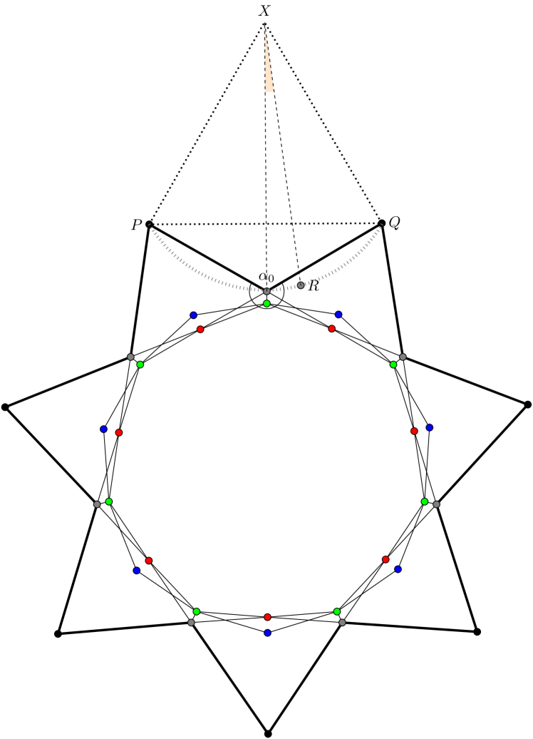
Figure 4.4.1. Note the dotted equilateral triangle $XPQ$ as well as the unique circular arc given by $P$, $R$ and $Q$. Denote by $\varphi$ the angle $OXR$ (where $O$ is the origin/center). The symmetric case is given by $\varphi=0$. To introduce deviation, we would slightly increase $\varphi$, and get a new position for $R$. This does not change the value of $\alpha_{0}$ (since we go along the circular arc). The same deviation is done at all seven grey points. This means that the star remains rotationally symmetric under a rotation by $360\degree/7$, but loses its symmetry under reflections.

4.5. Edges under deviation

As just established above, we only need to be concerned with the edges produced using the method of suspension. This section serves to support the following claim:

Whereas for $\varphi=0$, the geodesic nets $G_{i}(0)$ are highly symmetrical and many suspension edges overlap, for nonzero $\varphi\in(-\epsilon,\epsilon)$, all suspension edges of $G_{i}(\varphi)$ intersect transversally (if at all).

4.5.1. The sequence of suspension angles $\varphi_{i}$

To demonstrate this, we will study the sequence of suspension angles, which is defined as follows, based on the two types of suspension that we employ:

Definition 4.5.1 (Suspension angle for one-hook suspensions, layers $V_{i}$ for $i$ odd).

Whenever we do a one-hook suspension for a layer $V_{i}$, we are connecting a vertex $v$ to the closest vertex on the outer circle. Denote the center of the outer circle by $O$ and the hook by $P$. Then we define the suspension angle $\varphi_{i}$ to be the angle $\angle OPv$. For clarification, consider the figure on the right giving a positive suspension angle. Note that $\varphi_{i}$ depends only on the deviation $\varphi$ (which is the only free parameter of our construction) and that $\varphi_{i}(0)=0$ for all layers. We can define this suspension angle for all odd layers, even though in some cases we don’t need to suspend a vertex (if case A occurs).

Definition 4.5.2 (Suspension angle for two-hook suspensions, layers $V_{i}$ for $i$ even).

Whenever we do a two-hook suspension for a layer $V_{i}$, we are connecting a vertex $v$ to the closest two vertices on the outer circle $P$ and $Q$ through the Fermat point of $\Delta PvQ$, see the figure when defining two-hook suspension above). As before, we denote by $X$ the third vertex of the equilateral triangle $\Delta PQX$ used for the construction of the Fermat point. Let $O$ be the center of the outer circle. Then we define the suspension angle $\varphi_{i}$ to be the angle $\angle OXv$. For clarification, consider the figure on the right showing a positive suspension angle. Note that $\varphi_{i}$ depends only on the deviation $\varphi$ (which is the only free parameter of our construction) and that $\varphi_{i}(0)=0$ for all layers. Most importantly, for $i=0$ (the initial layer, aka the inner circle) the suspension angle is $\varphi_{0}(\varphi)=\varphi$. We can define this suspension angle for all even layers, even though in some cases we don’t need to suspend a vertex.

With this definition, we can now make the following observations:

Fact 4.5.3.

Consider $\varphi\in(-\epsilon,\epsilon)$ a geodesic net $G_{n}(\varphi)$ as constructed above with layers $V_{0},\dots,V_{n}$. Then

• As established before, only suspension edges could overlap/intersect non-transversally.

• For all one-hook suspensions (odd layers), only the edges going from vertices $v_{i}$, $v_{k}$ of two different layers to the same hook $P$ could overlap. But as long as $\varphi_{i}\neq\varphi_{k}$, they will not do so (this is apparent from the figure in the definition above).

• For all two-hook suspensions (even layers), only the edges suspending vertices $v_{i}$, $v_{k}$ of two different layers from the same two hooks $P$ and $Q$ could overlap. But as long as $\varphi_{i}\neq\varphi_{k}$, they will not do so (see figure 4.5.1).

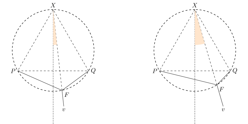
Figure 4.5.1. Construction of the Fermat point $F$ to suspend $v_{i}\in V_{i}$ from $P$ and $Q$. $\varphi_{i}$ is the angle between the axis of symmetry of $PQX$ and the segment $vX$. Observe: Whenever $\varphi_{i}$ (the marked suspension angle) is different, the segment $PF$ is at a different angle. The same is true for $QF$ and $vF$. So we only need to establish that $\varphi_{i}$ is different at every layer and this implies that none of the suspension edges overlap.

Note the following important observation:

Fact 4.5.4.

$G_{n}(\varphi)$ consists of finitely many layers, therefore $\varphi_{0},\varphi_{1},\dots,\varphi_{n}$ is a finite sequence.

Based on definitions 4.5.1, 4.5.2 and fact 4.5.3, we arrive at the following lemma:

Lemma 4.5.5.

If for any fixed $\varphi\in(-\epsilon,\epsilon)$, the sequence $\varphi_{i}(\varphi)$ never repeats itself, all edges of the resulting geodesic net $G_{n}(\varphi)$ intersect transversally (if at all). In other words, there are no edges with weight other than one.

Note that, in fact it would be enough if the $\varphi_{i}$ are different for the same parity (since even and odd layers never have suspension edges in common).

Based on symmetry (see also figure 4.3.2), we can observe

Fact 4.5.6.

$\varphi_{i}(0)=0$ for all $i$.

Also, since we established smooth dependence of the construction on the deviation $\varphi$ before and since this is in fact the only free parameter, we can consider the derivative of $\varphi_{i}(\varphi)$. We make the following conjecture:

Conjecture 4.5.7.

$\varphi_{i}^{\prime}(0)$ is a sequence that never repeats itself.

Keeping in mind that $\varphi_{i}$ is a finite sequence, the previous fact and conjecture (i.e. same value at $0$, but different derivatives) would then imply the following:

Conjecture 4.5.8.

For small nonzero $\varphi\in(-\epsilon,\epsilon)$, the sequence $\varphi_{i}(\varphi)$ never repeats itself. This implies that $G_{n}(\varphi)$ is a geodesic net for which all edges have weight one.

So this $G_{n}(\varphi)$ would in fact fulfill all required conditions:

1. There are $14$ unbalanced vertices.

2. For $n$ large enough, we can achieve an arbitrarily large number of balanced vertices.

3. All edges have weight one.

4.6. Studying the sequence $\varphi_{i}^{\prime}(0)$

So we are left with conjecture 4.5.7. For the remainder, we will consider statements we can make about the sequence $\varphi_{i}^{\prime}(0)$.

We will do the following:

• We will provide an explicit recursive formula for $\varphi_{i}^{\prime}(0)$.

• We will present numerical results that strongly suggest that conjecture 4.5.7 is true.

4.7. An explicit formula for $\varphi_{i}^{\prime}(0)$

In the following, all derivatives will be with respect to $\varphi$. First note, that $\varphi_{0}=\varphi$ and therefore obviously $\varphi_{0}^{\prime}(0)=1$. We will now find a recursive formula for $\varphi_{i}^{\prime}(0)$. The crucial question is how $\varphi_{i+1}^{\prime}(0)$ depends on $\varphi_{i}^{\prime}(0)$.

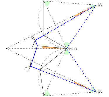
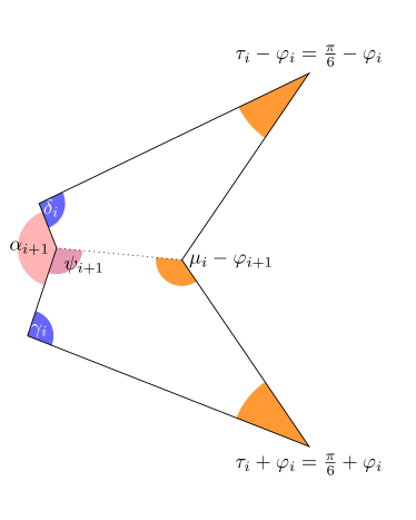
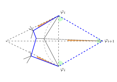
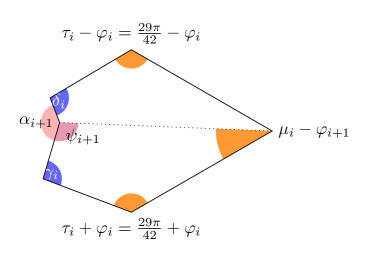
Figure 4.7.1. We want to relate $\varphi_{i+1}^{\prime}$ to $\varphi_{i}^{\prime}$. The upper pictures are considering the case $i$ even, the lower pictures are considering the case $i$ odd. All green angles are $60\degree$. $\mu$ is a constant angle. All dashed lines are stationary, all dotted and solid lines vary over a change of the deviation $\varphi$. The picture on the right extracts the blue hexagon out of the left picture. Note that in this example, $\varphi_{i}$ is positive whereas $\varphi_{i+1}$ is negative

Figure 4.7.1 shows the two cases for $i$ even and $i$ odd. Note that if $\varphi=0$, then the picture is symmetric along a horizontal reflection. In both cases, we get a hexagon made of two quadrilaterals.

In either case, by the angle sum in the lower quadrilateral:

$$\tau_{i}+\varphi_{i}+\gamma_{i}+\psi_{i+1}+\left(\mu_{i}-\varphi_{i+1}\right)=360\degree$$

Note that $\tau_{i}$ and $\mu_{i}$ are constants that don’t change under $\varphi$. Therefore, differentiation by $\varphi$ leads to:

$$\varphi_{i}^{\prime}+\gamma_{i}^{\prime}+\psi_{i+1}^{\prime}-\varphi_{i+1}^{\prime}=0\Rightarrow\varphi_{i+1}^{\prime}=\varphi_{i}^{\prime}+\gamma_{i}^{\prime}+\psi_{i+1}^{\prime}$$

In the appendix, we will establish the following relationships at $\varphi=0$.

$$\varphi_{0}^{\prime} =1\qquad\qquad\psi_{0}^{\prime}=\frac{1}{2}-\sin(\pi/6-\alpha_{0})$$

$$\varphi_{i+1}^{\prime} =\varphi_{i}^{\prime}+\gamma_{i}^{\prime}+\psi_{i+1}^{\prime}\qquad\qquad\psi_{i+1}^{\prime}=b_{i}\gamma_{i}^{\prime}+a_{i}\varphi_{i}^{\prime}\qquad\qquad\gamma_{i}^{\prime}=c_{i}\psi_{i}^{\prime}$$

The formulas for the coefficients make use of $x_{i}$ and $\alpha_{i}$, which were defined previously:

$$a_{i} =-\tan\frac{\alpha_{i+1}}{2}\left(\frac{\sin(\pi/7+\sigma_{i+1})\sin(\pi/7+\sigma_{i+1}+\tau_{i})}{\sin\tau_{i}}+\frac{\frac{1}{2}-\frac{\sin(\tau_{i}+2\pi/7+2\sigma_{i+1})}{2\sin\tau_{i}}}{\tan(\frac{\alpha_{i+1}}{2}-\sigma_{i+1})}\right)$$

$$b_{i} =-\frac{\tan\alpha_{i+1}/2}{\tan(\alpha_{i+1}/2-\sigma_{i+1})}\qquad\qquad c_{i}=\begin{cases}-1&\alpha_{i}>180\degree\\ \displaystyle\frac{2\cos\alpha_{i}/2}{1-2\cos\alpha_{i}/2}&\alpha_{i}<180\degree\end{cases}$$

$$\tau_{i} =\begin{cases}\pi/6&i\text{ even}\\ 29\pi/42&i\text{ odd}\\ \end{cases}\qquad\qquad\sigma_{i+1}=\begin{cases}\displaystyle\arctan\frac{\sin\pi/7}{\frac{\sin\alpha_{0}/2}{x_{i}\sin(\pi/7+\alpha_{0}/2)}-\cos\pi/7}&i\text{ even}\\ \displaystyle\arctan\frac{\sin\pi/7}{\frac{\sin\alpha_{0}/2}{x_{i}\sin(\pi/7+\alpha_{0}/2)}\frac{\sin(\pi/7+\pi/6)}{\sin\pi/6}-\cos\pi/7}&i\text{ odd}\end{cases}$$

4.8. Numerical consideration of the sequence $\varphi_{i}^{\prime}(0)$

While the formulas above are all explicit, they are arguably not very “handy” which makes understanding their behaviour a challenging task. Recall that all we need is that $\varphi_{i}^{\prime}(0)$ never repeats. This would then imply that a small deviation from $G_{n}(0)$ to $G_{n}(\varphi)$ would in fact split up all edges as required.

For a better understanding, we used MATLAB to compute the first items of the sequence. Figure 4.8.1 shows the first 100 elements of the sequence $\varphi_{i}^{\prime}(0)$, on a logarithmic scale. These calculations lead to the following observations, which in turn support conjecture 4.5.7, saying that $\varphi_{i}^{\prime}(0)$ doesn’t repeat:

• The magnitude of the sequence grows exponentially.

• The sequence seems to be generally increasing (i.e. increasing with a small number of exceptions)

• Since it is enough if the sequence differs for all even $i$ and for all odd $i$, we get additional “leeway”.

In fact, numerical evidence suggests that the first 100 elements of the sequence do not repeat. We computed the first 100 elements of $\varphi^{\prime}_{i}(0)$ with MATLAB using variable precision arithmetic, using between 10 and 100 significant digits. The following result remained stable under variable precision:

$$\min_{i\neq j}|\varphi^{\prime}_{i}(0)-\varphi^{\prime}_{j}(0)|\approx 3.743673268$$

This minimum is realized by $\varphi^{\prime}_{0}(0)$ and $\varphi^{\prime}_{2}(0)$.

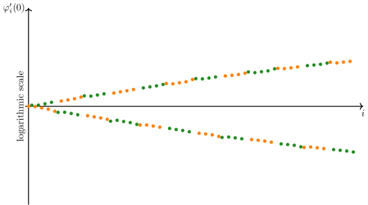
Figure 4.8.1. The first 100 values of $\varphi_{i}^{\prime}(0)$ on a logarithmic scale, calculated with $\alpha_{0}=88/21$. All points for $i$ even are marked in orange. All points for $i$ odd are marked in green.

5. Appendix: Finding the formulas for the sequence $\varphi_{i}^{\prime}(0)$

Consider figure 4.7.1 and the following formula we derived previously:

$$\varphi_{i+1}^{\prime}=\varphi_{i}^{\prime}+\gamma_{i}^{\prime}+\psi_{i+1}^{\prime}$$

In this appendix, we intend to do the following:

• Find the starting values of $\varphi_{0}^{\prime}(0)$ and $\psi_{0}^{\prime}(0)$.

• Establish that $\alpha_{i}^{\prime}(0)=0$ for all $i$.

• Derive a formula for $\gamma_{i}^{\prime}(0)$ in terms of $\psi_{i}^{\prime}(0)$.

• Derive a formula for $\psi_{i+1}^{\prime}(0)$ in terms of $\psi_{i}^{\prime}(0)$ and $\varphi_{i}^{\prime}(0)$.

5.1. Starting values

Since $\varphi$ is defined to be the suspension angle for the inner circle, which is the zeroth level (compare definition 4.5.2 and compare with the initial definition of the inner circle), $\varphi_{0}=\varphi$ and therefore

$$\varphi_{0}^{\prime}(0)=1$$

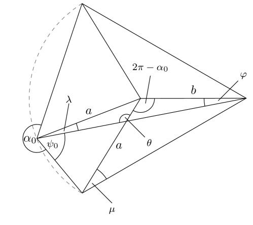
Figure 5.1.1. Dependence of $\psi_{0}$ on $\varphi$

To find $\psi_{0}^{\prime}(0)$, consider figure 5.1.1, more specifically the isosceles triangle with two sides of length $a$. Using angle sums in triangles:

$$\psi_{0}=(\pi-(\pi-\lambda-\theta))/2-\lambda=\theta/2-\lambda/2\ \Rightarrow\ \psi_{0}^{\prime}=\theta^{\prime}/2-\lambda^{\prime}/2$$

Finding $\lambda^{\prime}$. The law of sines, applied to the two triangles that share the common side of length $b$ but have two different sides of length $a$ gives us

$$\frac{\sin\lambda}{\sin\varphi}=\frac{b}{a}=\frac{\sin\mu}{\sin\pi/6}=2\sin\mu\ \Rightarrow\ \sin\lambda=2\sin\mu\sin\varphi\ \Rightarrow\ \cos\lambda\ \lambda^{\prime}=2\sin\mu\cos\varphi$$

At $\varphi=0$ we also have $\lambda=0$ and therefore $\lambda^{\prime}(0)=2\sin\mu=2\sin(\pi-\pi/6-(2\pi-\alpha_{0}))=2\sin(\pi/6-\alpha_{0})$.

Finding $\theta^{\prime}$. Using the angle sum in triangles, we get $\theta+\mu+\pi/6-\varphi=\pi$ and therefore $\theta^{\prime}=1$.

Combining these we arrive at $\psi_{0}^{\prime}(0)=\frac{1}{2}-\sin(\pi/6-\alpha_{0})$.

5.2. $\alpha_{i}^{\prime}(0)$ and $\gamma_{i}^{\prime}(0)$

Recall that $\alpha_{i}$ is the interior angle at the vertices $V_{i}$ of the 14-gon formed by $V_{i-1}$ and $V_{i}$. It is one of the two angles between the incoming edges at the vertex of a layer, before winging (see also methods 4.2.3 and 4.2.4 as well as the formulas in the proof of 4.3.2). Like all other angles, each $\alpha_{i}=\alpha_{i}(\varphi)$ is a smooth function of the deviation angle $\varphi$. Figures 4.7.1 and 5.2.1 show how $\gamma$ is one of the angles between an outgoing edge and the suspension edge, whereas $\psi$ is one of the angles between an incoming edge and the suspension edge (even if we do not suspend, as is the case for a degree $4$ vertex where $\alpha>180\degree$, we can still consider the angle compared to a hypothetical suspension edge.

Lemma 5.2.1.

For all $i=0,1,2,\dots$, we have the following relationships at $\varphi=0$

1. $\alpha_{i}^{\prime}=0$

2. $\gamma_{i}^{\prime}=c_{i}\psi_{i}^{\prime}$ where $c_{i}=\begin{cases}-1&\alpha_{i}>180\degree\\ \displaystyle\frac{2\cos\alpha_{i}/2}{1-2\cos\alpha_{i}/2}&\alpha_{i}<180\degree\end{cases}$

It is important to emphasize that these relationships between derivatives only hold at $\varphi=0$, which is, however, enough for us.

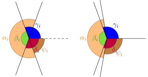
Figure 5.2.1. The angle relationships at a vertex of $V_{i}$ in the case of $\alpha_{i}>180\degree$ (left, winging a degree 2 vertex) and in the case of $\alpha_{i}<180\degree$ (right, winging a degree 3 vertex)

Proof.

1. For the base case, note that the inner circle is chosen precisely to ensure that $\alpha_{0}=88/21$ for any choice of $\varphi$. So $\alpha_{0}(\varphi)$ is constant and the base case follows.

   For the induction step, recall the following formulas (see proof of 4.3.2) for the symmetric case $\varphi=0$:

   $$\alpha_{i+1} =\frac{12\cdot 180\degree}{7}-\beta_{i}$$

   $$\beta_{i} =\begin{cases}360\degree-\alpha_{i}&\alpha_{i}>180\degree\quad\text{(winging of degree 2 vertex)}\\ 2\cdot\arccos(1/2-\cos(\alpha_{i}/2))&\alpha_{i}<180\degree\quad\text{(winging of degree 3 vertex)}\\ \end{cases}$$

   It is worth checking which of these formulas still apply in the deviated case $\varphi\neq 0$.

   • The relation $\alpha_{i+1}=\frac{12\cdot 180\degree}{7}-\beta_{i}$ remains unchanged, since the formula is based on the angle sum in the 14-gons during construction. Therefore $\alpha_{i+1}^{\prime}(0)=-\beta_{i}^{\prime}(0)$.

   • The formula for $\beta_{i}$ in the case of $\alpha_{i}>180\degree$ also applies to the non-symmetric case (see method 4.2.3). It follows that $\beta_{i}^{\prime}(0)=-\alpha_{i}^{\prime}(0)=0$ by induction hypothesis and we are done.

   • The formula for $\beta_{i}$ in the case of $\alpha_{i}<180\degree$, however, cannot be used for the asymmetric situation (as explained in method 4.2.4, it only works for the symmetric case).

   So we are left to show that $\beta_{i}^{\prime}(0)=0$ assuming that $\alpha_{i}^{\prime}(0)=0$ and $\alpha_{i}<180\degree$, but we can’t use the given formula.

   Instead, lets consider the right of figure 5.2.1, depicting this case. We ran rotate the vertex as depicted so that one edge is pointing to the right. Note that in the symmetric case, i.e. when $\varphi=0$, the picture is symmetric under reflection along the horizontal axis. Generally, though, this is not the case.

   The vertex is balanced, so we have

   $$[1,0]+[\cos\gamma_{i},\sin\gamma_{i}]+[\cos\delta_{i},-\sin\delta_{i}]+[\cos\psi_{i},-\sin\psi_{i}]+[\cos(\psi_{i}+\alpha_{i}),-\sin(\psi_{i}+\alpha_{i})]=[0,0]$$

   $$\Leftrightarrow \begin{cases}1+\cos\gamma_{i}+\cos\delta_{i}+\cos\psi_{i}+\cos(\psi_{i}+\alpha_{i})=0\\ \sin\gamma_{i}-\sin\delta_{i}-\sin\psi_{i}-\sin(\psi_{i}+\alpha_{i})=0\end{cases}$$

   We can derive everything with respect to $\varphi$ and arrive at

   $$-\gamma_{i}^{\prime}\sin\gamma_{i}-\delta_{i}^{\prime}\sin\delta_{i}-\psi_{i}^{\prime}\sin\psi_{i}-(\psi_{i}^{\prime}+\alpha_{i}^{\prime})\sin(\psi_{i}+\alpha_{i})=0$$

   $$\gamma_{i}^{\prime}\cos\gamma_{i}-\delta_{i}^{\prime}\cos\delta_{i}-\psi_{i}^{\prime}\cos\psi_{i}-(\psi_{i}^{\prime}+\alpha_{i}^{\prime})\cos(\psi_{i}+\alpha_{i})=0$$

   We are concerned with the derivatives at $\varphi=0$. As pointed out, the picture is symmetric in that case and we get $\gamma_{i}=\delta_{i}$ as well as $\psi_{i}+\alpha_{i}=2\pi-\psi_{i}$. By induction hypothesis, we also have $\alpha_{i}^{\prime}=0$. So we can simplify to

   $$-\gamma_{i}^{\prime}\sin\gamma_{i}-\delta_{i}^{\prime}\sin\gamma_{i}-\psi_{i}^{\prime}\sin\psi_{i}-\psi_{i}^{\prime}\sin(2\pi-\psi_{i})=0$$

   $$\gamma_{i}^{\prime}\cos\gamma_{i}-\delta_{i}^{\prime}\cos\gamma_{i}-\psi_{i}^{\prime}\cos\psi_{i}-\psi_{i}^{\prime}\cos(2\pi-\psi_{i})=0$$

   We can simplify further to

   $$-\gamma_{i}^{\prime}\sin\gamma_{i}-\delta_{i}^{\prime}\sin\gamma_{i}-\psi_{i}^{\prime}\sin\psi_{i}+\psi_{i}^{\prime}\sin\psi_{i}=0$$

   $$\gamma_{i}^{\prime}\cos\gamma_{i}-\delta_{i}^{\prime}\cos\gamma_{i}-\psi_{i}^{\prime}\cos\psi_{i}-\psi_{i}^{\prime}\cos\psi_{i}=0$$

   Note that $\gamma_{i}$ can’t be a multiple of $\pi$ at $\varphi=0$ since that would imply $\beta_{i}=0$ or $\beta_{i}=2\pi$ which is never the case as established previously. So $\sin\gamma_{i}\neq 0$ and the two equations do in fact simplify to

   $$\gamma_{i}^{\prime}+\delta_{i}^{\prime} =0$$

   $$(\gamma_{i}^{\prime}-\delta_{i}^{\prime})\cos\gamma_{i} =2\psi_{i}^{\prime}\cos\psi_{i}$$

   As is clear from figure 5.2.1, $\beta_{i}=2\pi-(\gamma_{i}+\delta_{i})$. Therefore $\beta_{i}^{\prime}=-(\gamma_{i}^{\prime}+\delta_{i}^{\prime})=0$ as required.

2. If $\alpha_{i}>180\degree$ consider the left of figure 5.2.1 from which it is clear that $\gamma_{i}=180\degree-\psi_{i}$. It follows that $\gamma_{i}^{\prime}=-\psi_{i}^{\prime}$ as stated (this relationship, in fact, would be true for any $\varphi\in(-\epsilon,\epsilon)$, not just for $\varphi=0$).

   If $\alpha_{i}<180\degree$, we have just established the following at $\varphi=0$

   $$\gamma_{i}^{\prime}+\delta_{i}^{\prime}=0\text{ and }(\gamma_{i}^{\prime}-\delta_{i}^{\prime})\cos\gamma_{i}=2\psi_{i}^{\prime}\cos\psi_{i}\quad\Rightarrow\quad 2\gamma_{i}^{\prime}\cos\gamma_{i}=2\psi_{i}^{\prime}\cos\psi_{i}\quad\Rightarrow\quad\gamma_{i}^{\prime}=\frac{\cos\psi_{i}}{\cos\gamma_{i}}\psi_{i}^{\prime}$$

   Furthermore, again due to symmetries at $\varphi=0$

   $$\cos\gamma_{i} =\cos(\pi-\beta_{i}/2)=-\cos(\beta_{i}/2)=-\cos\left(\frac{2\arccos(1/2-\cos(\alpha_{i}/2))}{2}\right)=-(1/2-\cos\alpha_{i}/2)$$

   $$\cos\psi_{i} =\cos(\pi-\alpha_{i}/2)=-\cos\alpha_{i}/2$$

   Combining these equations, we arrive at $\gamma_{i}^{\prime}=c_{i}\psi_{i}^{\prime}$ with $c_{i}=\displaystyle\frac{2\cos\alpha_{i}/2}{1-2\cos\alpha_{i}/2}$.

∎

5.3. $\tau_{i}$ and $\sigma_{i}$

$\tau_{i}$ is the “reference angle” from which the suspension angle $\varphi_{i}$ is measured. Consider the $14$-gon formed by the two outer sides of each of the seven equilateral triangles built on the outer circle. The interior angle at seven corners is $\pi/3$, the interior angle at the other seven corners is $29\pi/21$. These are the values for $2\cdot\tau_{i}$ even and odd respectively.

The angle $\sigma_{i+1}$ is depicted in figure 5.4.1. It changes under deviation, but at $\varphi=0$ it can be directly calculated from the sequence of $x_{i}$. If $i$ is even, consider figure 5.4.2. Note that $\sigma_{i+1}$ is one of the angles in a triangle with side $x_{i}$ and angle $\pi/7$. Since $\sigma_{i+1}$ is the angle at a vertex of the outer circle, we know one more side of the triangle. Recall that the inner circle is fixed at radius $1$ and consider figure 4.2.1, giving the other side as $\frac{\sin\alpha_{0}/2}{\sin(\pi/7+\alpha_{0}/2)}$. Using the law of sines, we get:

$$\sin\sigma_{i+1}=x_{i}\sin(\sigma_{i+1}+\pi/7)\frac{\sin(\pi/7+\alpha_{0}/2)}{\sin\alpha_{0}/2}$$

If $i$ is odd, a similar argument yields

$$\sin\sigma_{i+1}=x_{i}\sin(\sigma_{i+1}+\pi/7)\frac{\sin(\pi/7+\alpha_{0}/2)}{\sin\alpha_{0}/2}\frac{\sin\pi/6}{\sin(\pi/7+\pi/6)}$$

which is based on the fact that the additional vertex of $\sigma_{i}$ is at radius $\frac{\sin\alpha_{0}/2}{\sin(\pi/7+\alpha_{0}/2)}\frac{\sin(\pi/7+\pi/6)}{\sin\pi/6}$.

Since $\sigma_{i+1}<90\degree$, we can solve both equations for $\sigma_{i+1}$ and get

$$\sigma_{i+1}=\begin{cases}\displaystyle\arctan\frac{\sin\pi/7}{\frac{\sin\alpha_{0}/2}{x_{i}\sin(\pi/7+\alpha_{0}/2)}-\cos\pi/7}&i\text{ even}\\ \displaystyle\arctan\frac{\sin\pi/7}{\frac{\sin\alpha_{0}/2}{x_{i}\sin(\pi/7+\alpha_{0}/2)}\frac{\sin(\pi/7+\pi/6)}{\sin\pi/6}-\cos\pi/7}&i\text{ odd}\end{cases}$$

5.4. The formula for $\psi_{i}^{\prime}(0)$

We are left to establish the following

Lemma 5.4.1.

For all $i=0,1,2,\dots$ at $\varphi=0$, we have $\psi_{i+1}^{\prime}=b_{i}\gamma_{i}^{\prime}+a_{i}\varphi_{i}^{\prime}$ where

$$b_{i} =-\frac{\tan\frac{\alpha_{i+1}}{2}}{\tan(\frac{\alpha_{i+1}}{2}-\sigma_{i+1})}\qquad\qquad$$

$$a_{i} =-\tan\frac{\alpha_{i+1}}{2}\left(\frac{\sin(\pi/7+\sigma_{i+1})\sin(\pi/7+\sigma_{i+1}+\tau_{i})}{\sin\tau_{i}}+\frac{\frac{1}{2}-\frac{\sin(\tau_{i}+2\pi/7+2\sigma_{i+1})}{2\sin\tau_{i}}}{\tan(\frac{\alpha_{i+1}}{2}-\sigma_{i+1})}\right)$$

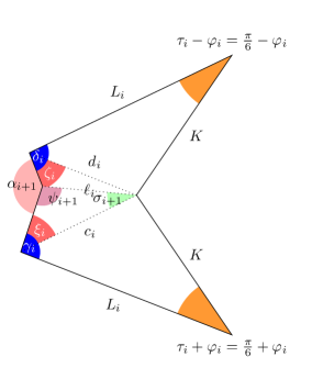
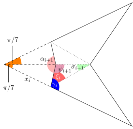
Figure 5.4.1. A detailed overview of a part of figure 4.7.1

Proof.

Consider the two cases in figure 4.7.1. We will cover the first case in detail ($i$ even). The other case, as given the lower of the two figures, can be deduced in the same way (the pictures only differ in the size of the angles, the underlying setup of polygons is the same). For this first case, figure 5.4.1 gives a more detailed overview.

$\psi_{i}$ is a particular angle in the given hexagon. The angles $\kappa_{i}$ and $\tau_{i}$ don’t change under $\varphi$ and neither does $K$ (it is the length of the sides of the equilateral triangles over the outer circle). Note the following: If we consider these angles and lengths

• The lengths $L_{i}$

• The angles $\varphi_{i}$, $\gamma_{i}$, $\delta_{i}$

then there is a one-to-one correspondence (within an open set) between tuples $(L_{i},\varphi_{i},\gamma_{i},\delta_{i})$ and hexagons.

Also note that the pictures is symmetric at $\varphi=0$, implying $\gamma_{i}(0)=\delta_{i}(0)$ and $\varphi_{i}(0)=0$. Since these quantities uniquely define the hexagon and since $\psi_{i+1}$ is an angle defined by the hexagon, we arrive at

$$\psi_{i+1}^{\prime}=\frac{\partial\psi_{i+1}}{\partial L_{i}}L_{i}^{\prime}+\frac{\partial\psi_{i+1}}{\partial\gamma_{i}}\gamma_{i}^{\prime}+\frac{\partial\psi_{i+1}}{\partial\delta_{i}}\delta_{i}^{\prime}+\frac{\partial\psi_{i+1}}{\partial\varphi_{i}}\varphi_{i}^{\prime}$$

As usual, we consider these derivatives at $\varphi=0$. The proof of the previous lemma established that in that case $\gamma_{i}^{\prime}=-\delta_{i}^{\prime}$. Also note that in the symmetric picture, a change in $L_{i}$ will not affect $\psi_{i}$. Therefore $\frac{\partial\psi_{i+1}}{\partial L_{i}}$ at $\varphi=0$. Combining all these, we arrive at

$$\psi_{i+1}^{\prime}=\left(\frac{\partial\psi_{i+1}}{\partial\gamma_{i}}-\frac{\partial\psi_{i+1}}{\partial\delta_{i}}\right)\gamma_{i}^{\prime}+\frac{\partial\psi_{i+1}}{\partial\varphi_{i}}\varphi_{i}^{\prime}$$

So we are left to show that

1. $b_{i}=\left(\frac{\partial\psi_{i+1}}{\partial\gamma_{i}}-\frac{\partial\psi_{i+1}}{\partial\delta_{i}}\right)=-\frac{\tan\frac{\alpha_{i+1}}{2}}{\tan(\frac{\alpha_{i+1}}{2}-\sigma_{i+1})}$

2. $a_{i}=\frac{\partial\psi_{i+1}}{\partial\varphi_{i}}=-\frac{\tan\frac{\alpha_{i+1}}{2}}{\sin\tau_{i}}\left(\sin(\pi/7+\sigma_{i+1})\sin(\pi/7+\sigma_{i+1}+\tau_{i})+\frac{-\sin\tau_{i}+\sin(\tau_{i}+2\pi/7+2\sigma_{i+1})}{2\tan(\frac{\alpha_{i+1}}{2}-\sigma_{i+1})}\right)$

To do so, we will make extensive use of trigonometric identities and laws.

The law of sines provides

$$c_{i}\frac{\sin\xi_{i}}{\sin\psi_{i+1}}=\ell_{i}=d_{i}\frac{\sin\zeta_{i}}{\sin(4\pi-\gamma_{i}-\delta_{i}-(\tau_{i}+\varphi_{i})-(\tau_{i}-\varphi_{i})-(2\pi-\kappa_{i})-\psi_{i+1})}$$

$$\Rightarrow c_{i}\sin\xi_{i}\sin(4\pi-\gamma-\delta-2\tau_{i}-(2\pi-\kappa_{i})-\psi_{i+1})=d_{i}\sin\zeta_{i}\sin\psi_{i+1}$$

1. Deriving with respect to $\gamma_{i}$ yields

   $$\text{derivatives w.r.t. }\gamma_{i}\left\{\begin{array}[]{lll}c_{i}\cos\xi_{i}\ \xi_{i}^{\prime}\sin(4\pi-\gamma_{i}-\delta_{i}-2\tau_{i}-(2\pi-\kappa_{i})-\psi_{i+1})\\ +c_{i}\sin\xi_{i}\cos(4\pi-\gamma_{i}-\delta_{i}-2\tau_{i}-(2\pi-\kappa_{i})-\psi_{i+1})\ (-1-\psi_{i+1}^{\prime})\\ =d_{i}\sin\zeta_{i}\ \cos\psi_{i+1}\ \psi_{i+1}^{\prime}\end{array}\right.$$

   We are considering values at $\varphi=0$. Due to symmetry

   $$\xi_{i} =\zeta_{i} c_{i} =d_{i} \psi_{i+1} =4\pi-\gamma-\delta-2\tau_{i}-(2\pi-\kappa_{i})-\psi_{i+1}=\pi-\frac{\alpha_{i+1}}{2}$$

   Also, $\xi_{i}=\gamma_{i}+\theta$ where $\theta$ is an angle that doesn’t change under $\gamma$. Therefore (since we are currently considering derivatives with respect to $\gamma_{i}$) we have $\xi_{i}^{\prime}=1$. Combining all these, we arrive at:

   $$\text{derivatives w.r.t. }\gamma_{i}\left\{\begin{array}[]{lll}c_{i}\cos\xi_{i}\ \sin\frac{\alpha_{i+1}}{2}-c_{i}\sin\xi_{i}\ \cos\frac{\alpha_{i+1}}{2}\ (-1-\psi_{i+1}^{\prime})\\ =-c_{i}\sin\xi_{i}\ \cos\frac{\alpha_{i+1}}{2}\ \psi_{i+1}^{\prime}\end{array}\right.$$

   This can be simplified to

   $$\text{derivatives w.r.t. }\gamma_{i}\left\{\begin{array}[]{lll}\cot\xi_{i}\ \tan\frac{\alpha_{i+1}}{2}-(-1-\psi_{i+1}^{\prime})=-\psi_{i+1}^{\prime}\end{array}\right.$$

   So we finally arrive at

   $$\frac{\partial\psi_{i+1}}{\partial\gamma_{i}}=-\frac{1}{2}\left(\cot\xi_{i}\tan\frac{\alpha_{i+1}}{2}+1\right)$$

   Note that at $\varphi=0$, we have $\pi=\xi_{i}+\sigma_{i+1}+\psi_{i+1}=\xi_{i}+\sigma_{i+1}+\pi-\frac{\alpha_{i+1}}{2}$ and therefore $\cot\xi_{i}=\cot(\frac{\alpha_{i+1}}{2}-\sigma_{i+1})$, so we can rewrite this as

   $$\frac{\partial\psi_{i+1}}{\partial\gamma_{i}}=-\frac{1}{2}\left(\frac{\tan\frac{\alpha_{i+1}}{2}}{\tan(\frac{\alpha_{i+1}}{2}-\sigma_{i+1})}+1\right)$$

   Very similar deductions based on derivatives with respect to $\delta_{i}$ allow us to arrive at

   $$\frac{\partial\psi_{i+1}}{\partial\delta_{i}}=\frac{1}{2}\left(\frac{\tan\frac{\alpha_{i+1}}{2}}{\tan(\frac{\alpha_{i+1}}{2}-\sigma_{i+1})}-1\right)$$

   The claim for $b_{i}$ follows.

2. We return to the identity based on the law of sines from above, but will now consider derivatives with respect to $\varphi_{i}$. Note that this time, $c_{i}$, $d_{i}$, $\xi_{i}$ and $\zeta_{i}$ vary whereas $\gamma_{i}$ and $\delta_{i}$ are constant.

   $$\text{derivatives w.r.t. }\varphi_{i}\left\{\begin{array}[]{lll}c_{i}^{\prime}\sin\xi_{i}\sin(4\pi-\gamma_{i}-\delta_{i}-2\tau_{i}-(2\pi-\kappa_{i})-\psi_{i+1})\\ +c_{i}\cos\xi_{i}\ \xi_{i}^{\prime}\sin(4\pi-\gamma_{i}-\delta_{i}-2\tau_{i}-(2\pi-\kappa_{i})-\psi_{i+1})\\ +c_{i}\sin\xi_{i}\cos(4\pi-\gamma_{i}-\delta_{i}-2\tau_{i}-(2\pi-\kappa_{i})-\psi_{i+1})\ (-\psi_{i+1}^{\prime})\\ =d_{i}^{\prime}\sin\zeta_{i}\sin\psi_{i+1}+d_{i}\cos\zeta_{i}\ \zeta_{i}^{\prime}\sin\psi_{i+1}+d_{i}\sin\zeta_{i}\cos\psi_{i+1}\ \psi_{i+1}^{\prime}\end{array}\right.$$

   We are considering values at $\varphi=0$. Due to symmetry

   $$\xi_{i} =\zeta_{i} c_{i} =d_{i} c_{i}^{\prime} =-d_{i}^{\prime} \xi_{i}^{\prime} =-\zeta_{i}^{\prime} \psi_{i+1} =4\pi-\gamma_{i}-\delta_{i}-2\tau_{i}-(2\pi-\kappa_{i})-\psi_{i+1}=\pi-\frac{\alpha_{i+1}}{2}$$

   Combining all these, we arrive at

   $$\text{derivatives w.r.t. }\varphi_{i}\left\{\begin{array}[]{lll}c_{i}^{\prime}\sin\xi_{i}\sin\frac{\alpha_{i+1}}{2}+c_{i}\cos\xi_{i}\ \xi_{i}^{\prime}\sin\frac{\alpha_{i+1}}{2}+c_{i}\sin\xi_{i}\cos\frac{\alpha_{i+1}}{2}\ \psi_{i+1}^{\prime}\\ =-c_{i}^{\prime}\sin\xi_{i}\sin\frac{\alpha_{i+1}}{2}-c_{i}\cos\xi_{i}\ \xi_{i}^{\prime}\sin\frac{\alpha_{i+1}}{2}-c_{i}\sin\xi_{i}\cos\frac{\alpha_{i+1}}{2}\ \psi_{i+1}^{\prime}\end{array}\right.$$

   And therefore

   $$\text{derivatives w.r.t. }\varphi_{i}\left\{\begin{array}[]{lll}c_{i}^{\prime}\sin\xi_{i}\sin\frac{\alpha_{i+1}}{2}+c_{i}\cos\xi_{i}\ \xi_{i}^{\prime}\sin\frac{\alpha_{i+1}}{2}+c_{i}\sin\xi_{i}\cos\frac{\alpha_{i+1}}{2}\ \psi_{i+1}^{\prime}=0\end{array}\right.$$

   This can be solved for

   $$\text{derivatives w.r.t. }\varphi_{i}\left\{\begin{array}[]{lll}\psi_{i+1}^{\prime}=-\tan\frac{\alpha_{i+1}}{2}\left(\frac{c_{i}^{\prime}}{c_{i}}+\cot\xi_{i}\ \xi_{i}^{\prime}\right)\end{array}\right.$$

   We now have to find $c_{i}^{\prime}/c_{i}$ and $\xi_{i}^{\prime}$. We start with $c_{i}^{\prime}/c_{i}$. Recall that we are still considering derivatives with respect to $\varphi_{i}$. The law of cosines gives us

   $$\text{derivatives w.r.t. }\varphi_{i}\left\{\begin{array}[]{lll}c_{i}^{2}=K^{2}+L_{i}^{2}-2KL_{i}\cos(\tau_{i}+\varphi_{i})\\ \Rightarrow 2c_{i}c_{i}^{\prime}=2KL_{i}\sin(\tau_{i}+\varphi_{i})\\ \Rightarrow\frac{c_{i}^{\prime}}{c_{i}}=\frac{K}{c_{i}}\frac{L_{i}}{c_{i}}\sin(\tau_{i}+\varphi_{i})\end{array}\right.$$

   At $\varphi=0$, we have

   $$\varphi_{i} =0 \frac{K}{c_{i}} =\frac{\sin(\gamma_{i}-\xi_{i})}{\sin\tau_{i}} \frac{L_{i}}{c_{i}} =\frac{\sin(\pi-(\gamma_{i}-\xi_{i})-\tau_{i})}{\sin\tau_{i}}=\frac{\sin(\gamma_{i}-\xi_{i}+\tau_{i})}{\sin\tau_{i}}$$

   We finish with finding $\xi_{i}^{\prime}$ (still as a derivative with respect to $\varphi_{i}$). We invoke the law of tangents for the triangle with sides $c_{i}$, $K$, $L_{i}$.

   $$\frac{L_{i}-K}{L_{i}+K}=\frac{\tan(\frac{1}{2}(\pi-(\tau_{i}+\varphi_{i})-(\gamma_{i}-\xi_{i})-(\gamma_{i}-\xi_{i}))}{\tan(\frac{1}{2}(\pi-(\tau_{i}+\varphi_{i})-(\gamma_{i}-\xi_{i})+(\gamma_{i}-\xi_{i}))}=\frac{\tan(\frac{1}{2}(\pi-\tau_{i}-\varphi_{i}-2(\gamma_{i}-\xi_{i})))}{\tan(\frac{1}{2}(\pi-\tau_{i}-\varphi_{i}))}$$

   Note that the left-hand side doesn’t change under a change of $\varphi_{i}$. So if we derive (and subsequently multiply by the denominator), we get

   $$\text{derivatives w.r.t. }\varphi_{i}\left\{\begin{array}[]{lll}0=\sec^{2}(\frac{1}{2}(\pi-\tau_{i}-\varphi_{i}-2(\gamma_{i}-\xi_{i})))(-1+2\xi_{i}^{\prime})\tan(\frac{1}{2}(\pi-\tau_{i}-\varphi_{i}))\\ +\tan(\frac{1}{2}(\pi-\tau_{i}-\varphi_{i}-2(\gamma_{i}-\xi_{i})))\sec^{2}(\frac{1}{2}(\pi-\tau_{i}-\varphi_{i}))\end{array}\right.$$

   Elementary trigonometric identities lead us to

   $$\text{derivatives w.r.t. }\varphi_{i}\left\{\begin{array}[]{lll}\displaystyle\xi_{i}^{\prime}=\frac{1}{2}-\frac{\sin(\pi-\tau_{i}-\varphi_{i}-2(\gamma_{i}-\xi_{i}))}{2\sin(\pi-\tau_{i}-\varphi_{i})}\end{array}\right.$$

   At $\varphi=0$, we have $\varphi_{i}=0$. So we get

   $$\text{derivatives w.r.t. }\varphi_{i}\left\{\begin{array}[]{lll}\displaystyle\xi_{i}^{\prime}=\frac{1}{2}-\frac{\sin(\tau_{i}+2(\gamma_{i}-\xi_{i}))}{2\sin\tau_{i}}\end{array}\right.$$

   We now have explicit formulas for $c_{i}^{\prime}/c_{i}$ as well as $\xi_{i}^{\prime}$. Combining the above results and using the following two identities at $\varphi=0$ (see figure 5.4.2):

   $$\xi_{i} =\pi-\psi_{i+1}-\sigma_{i+1}=\frac{\alpha_{i+1}}{2}-\sigma_{i+1} \pi-(\gamma_{i}-\xi_{i})+\pi/7+\sigma_{i+1}=\pi\ \Rightarrow\ \gamma_{i}-\xi_{i} =\pi/7+\sigma_{i+1}$$

   we can finally write

   $$\frac{\partial\psi_{i+1}}{\partial\varphi_{i}}=-\tan\frac{\alpha_{i+1}}{2}\left(\frac{\sin(\pi/7+\sigma_{i+1})\sin(\pi/7+\sigma_{i+1}+\tau_{i})}{\sin\tau_{i}}+\frac{\frac{1}{2}-\frac{\sin(\tau_{i}+2\pi/7+2\sigma_{i+1})}{2\sin\tau_{i}}}{\tan(\frac{\alpha_{i+1}}{2}-\sigma_{i+1})}\right)$$

∎

Figure 5.4.2. A figure showing the relationship between angles at $\varphi=0$ for $i$ even.

6. Acknowledgements

This research has been partially supported by A. Nabutovsky’s NSERC Discovery grant and F. Parsch’s Vanier Canada Graduate Scholarship. The authors would like to thank Adam Stinchcombe for valuable help with variable precision arithmetic in MATLAB.

References

- [AA76] W. K. Allard and F. J. Almgren, Jr., The structure of stationary one dimensional varifolds with positive density, Invent. Math. 34 (1976), no. 2, 83–97.
- [BK] Spencer Becker-Kahn, unpublished.
- [GL] Larry Guth and Yevgeny Liokumovich, in preparation.
- [Hep99] Aladár Heppes, On the partition of the -sphere by geodesic nets, Proc. Amer. Math. Soc. 127 (1999), no. 7, 2163–2165.
- [HM96] Joel Hass and Frank Morgan, Geodesic nets on the -sphere, Proc. Amer. Math. Soc. 124 (1996), no. 12, 3843–3850.
- [IT94] Alexandr O. Ivanov and Alexei A. Tuzhilin, Minimal networks, CRC Press, Boca Raton, FL, 1994.
- [IT16] Alexander O. Ivanov and Alexey A. Tuzhilin, Minimal networks: a review, Advances in dynamical systems and control, Stud. Syst. Decis. Control, vol. 69, Springer, 2016, pp. 43–80.
- [Mem15] Yashar Memarian, On the maximum number of vertices of critically embedded graphs, International Electronic Journal of Geometry 8 (2015), 168 – 180.
- [NR07] Alexander Nabutovsky and Regina Rotman, Shapes of geodesic nets, Geom. Topol. 11 (2007), 1225–1254.
- [Par18] Fabian Parsch, Geodesic nets with three boundary vertices, arXiv:1803.03728 (2018), 1–37.
- [Par19] by same author, An example for a nontrivial irreducible geodesic net in the plane, arXiv:1902.07872 (2019), 1–7.
- [Rot] Regina Rotman, Short wide geodesic loops on closed riemannian manifolds, in preparation.
- [Rot11] by same author, Flowers on Riemannian manifolds, Math. Z. 269 (2011), no. 1-2, 543–554.