Solitary waves on rotational flows with an interior stagnation point

Abstract

The two-dimensional free-boundary problem describing steady gravity waves with vorticity on water of finite depth is considered. Under the assumption that the vorticity is a negative constant whose absolute value is sufficiently large, we construct a solution with the following properties. The corresponding flow is unidirectional at infinity and has a solitary wave of elevation as its upper boundary; under this unidirectional flow, there is a bounded domain adjacent to the bottom, which surrounds an interior stagnation point and is divided into two subdomains with opposite directions of flow by a critical level curve connecting two stagnation points on the bottom.

Keywords: Steady water waves, constant negative vorticity, periodic waves, solitary wave, shear flow

1 Introduction

In the present paper, we consider the problem describing two-dimensional gravity waves travelling on a flow of finite depth. For an ideal fluid of constant density, say water, the effects of surface tension are neglected, whereas the flow is assumed to be rotational with a constant vorticity; this, according to observations, is the type of motion commonly occurring in nature (see, for example, Swan et al. (2001); Thomas (1981) and references cited therein). Also, it is assumed that the reference frame is moving with the wave so that the relative velocity field is stationary. Our aim is to consider a new class of solitary waves each having a cat’s-eye—a region of closed streamlines surrounding a stagnation point. Previously, this kind of behaviour was known only for periodic waves with vorticity.

The mathematical theory of two-dimensional solitary waves on irrotational flows goes back to the discovery of John Stcott Russell, who was the first to observe in 1834 and subsequently to analyse a solitary wave of elevation; see Russell (1844). The existence of the latter was justified mathematically by Boussinesq in 1877 and rediscovered by Korteweg and de Vries in 1895. The existence of solitary waves in the framework of the full water wave problem is far more complicated and the first proofs were obtained much later (by Lavrentiev (1954) and Friedrichs & Hyers (1954)). Modern proofs by Thomas Beale (1977) and Mielke (1988) use the Nash–Moser implicit function theorem and a dynamical system approach respectively. All these papers deal only with waves of small amplitude, whereas Amick & Toland (1981b) constructed large-amplitude solitary waves using global bifurcation theory and then proved the existence of a limiting wave of the extreme form, that is, having an angled crest, see Amick et al. (1982). All solitary waves considered in these papers are of positive elevation, symmetric and monotone on each side of the crest, see Craig & Sternberg (1988); McLeod (1984). The corresponding flows, being irrotatonal, have a simple structure of streamlines: they are unbounded curves similar (diffeomorphic) to the free surface profile. For all unidirectional waves with vorticity (when the horizontal component $u$ of the relative velocity field has a constant sign everywhere in the fluid), the latter property is also true. Essentially, this forbids the presence of critical layers and stagnation points.

The first construction of unidirectional small-amplitude solitary waves with vorticity was given by Ter-Krikorov (1962), whereas Benjamin (1962) obtained an approximate form of the wave profile which is the same as in the irrotational case. However, the relationships between the wave amplitude, the length scale and the propagation velocities depend on the primary velocity distribution in a complicated way. Much later, Hur (2008) and Groves & Wahlén (2008) obtained new results on this topic. The latter authors also considered solitary waves with vorticity in the presence of surface tension Groves & Wahlén (2007). The method used in Groves & Wahlén (2007, 2008), known as spatial dynamics, is essentially an infinite-dimensional version of the centre-manifold reduction which is known as spatial dynamics because is applied to a Hamiltonian system with the horizontal spatial coordinate playing the role of time. The first use of this method in the water-wave theory is due to Kirchgässner (1988, 1982) (see also Mielke (1986, 1988, 1991)), whereas an application of spatial dynamics to three-dimensional waves is given in Groves & Nilsson (2018) (see also references cited therein). So far, use of spatial dynamics was restricted exclusively to small-amplitude waves. Recently, Wheeler (2013) examined waves of large amplitude, but, like in the irrotational case, all solitary-wave solutions have the same structure of streamlines, that is, are symmetric and of positive elevation; see Hur (2008); Wheeler (2015); Kozlov et al. (2015, 2017). Thus, looking for a more complicated geometry of solitary waves, it is natural to consider flows with stagnation points and critical levels within the fluid domain. As in Wahlén (2009), by a critical level we mean a curve, where the horizontal component of velocity vanishes.

The simplest case of flows with critical levels is that of constant negative vorticity, and this has several advantages. Flows with constant vorticity are easier tractable mathematically and they are of substantial practical importance being pertinent to a wide range of hydrodynamic phenomena (see Constantin et al. (2016), p. 196). A new feature of laminar flows with constant vorticity (compared with irrotational ones) is that there are flows with critical levels. Moreover, it was shown by Wahlén (2009) that small perturbations of these parallel flows are periodic waves with arrays of cat’s-eye vortices—regions of closed streamlines surrounding stagnation points. An extension to periodic waves of large amplitude with critical layers is given in Constantin et al. (2016) (it includes overhanging waves). Despite the fact that waves considered in Wahlén (2009) and Constantin et al. (2016) have critical layers, the geometry of free surface profiles is still simple: symmetric about every crest and trough and monotone in between (just like that of the classical Stokes waves). Examples of more complicated wave profiles are known (see Ehrnström et al. (2011); Aasen & Varholm (2017); Kozlov & Lokharu (2017, 2019)), but for their construction the vorticity distribution must be at least linear. It should be emphasised that all theoretical studies of waves with critical layers were restricted so far to the periodic setting.

In the 1980s and 1990s, much attention was devoted to numerical computation of various solitary waves on flows with constant vorticity; see the papers Vanden-Broeck (1994, 1995) and references cited therein. In particular, an interesting family of solitary-wave profiles was obtained in the second of these papers; it approaches a singular one with trapped circular bulb at the crest which happens as the gravity acceleration tends to zero. However, no attempt was made to find bottom or interior stagnation points.

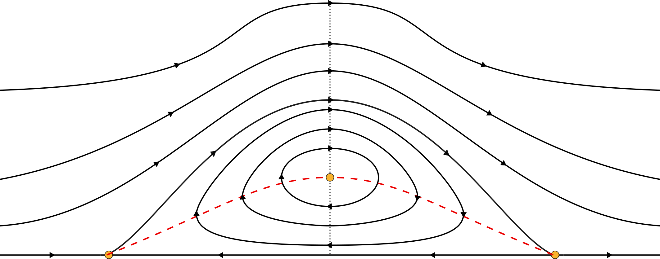
Figure 1: A sketch of the streamline pattern. Solid dots denote stagnation points and the dashed line shows the critical level, where the horizontal component of velocity vanishes. Another line connecting the bottom stagnation points is the critical streamline; the direction of streaming is indicated by arrows.

In the present paper, a new family of solitary waves is constructed for large negative values of the constant vorticity. All these waves have a remarkable property: the corresponding flow is unidirectional at both infinities, but there is a cat’s-eye vortex centred below the wave crest; see Figure 1. (The term was coined by Kelvin in his considerations of a shear flow having this pattern of streamlines; see Majda & Bertozzi (2002), pp. 53–54.) The vortex is bottom-adjacent and separated from the unidirectional flow above it by a critical streamline connecting two stagnation points on the bottom. Every solitary wave under consideration is obtained as a long-wave limit of Stokes wave-trains; in this aspect, our result is similar to that of Amick & Toland (1981a), who dealt with the irrotational case. However, Stokes waves has a cat’s-eye vortex centred below each crest in our case. For a sketch of the corresponding streamline pattern see the top Figure 4 below, whereas examples computed numerically are presented in Ribeiro et al. (2017), pp. 803–804. As the wavelength goes to infinity, these vortices does not shrink, which is different from the case of small-amplitude waves, whose sketch is plotted by Wahlén (2009) in his Figure 1. A sketch of streamlines corresponding to our solitary wave is plotted in Figure 1, where the solid dots denote stagnation points. Moreover, the dashed line shows the critical level along which the horizontal component of velocity vanishes and the critical streamline located above the critical level also connects the two bottom stagnation points; the direction of streaming is indicated by arrows.

It should be emphasised that small-amplitude solitary waves constructed in this paper cannot be captured by applying spatial dynamics directly because in a certain sense the problem turns into a singular one for large values of the vorticity. Thus, an appropriate scaling and a careful analysis are required prior spatial dynamics can be used.

The plan of the paper is as follows. Statement of the problem and formulation of main result are given in Subsection 1.1. Then, in Section 2, the problem is scaled and reformulated in a suitable way. After that, in Section 3, it is reduced to a finite-dimensional Hamiltonian system and Theorem 3 provides the existence of solitary waves. Then the main Theorem 1 is proved in Section 4.

1.1 Statement of the problem and formulation of the main result

Let an open channel of uniform rectangular cross-section be bounded from below by a horizontal rigid bottom and let water occupying the channel be bounded from above by a free surface not touching the bottom. The surface tension is neglected on the free surface, whereas the pressure is assumed to be cons tant there. In appropriate Cartesian coordinates $(X,Y)$, the bottom coincides with the $X$-axis and gravity acts in the negative $Y$-direction. We choose the frame of reference so that the velocity field is time-independent as well as the unknown free-surface profile. The latter is assumed to be the graph of $Y=\eta(X)$, $X\in\mathbb{R}$, where $\eta$ is a positive function. The water motion is supposed to be two-dimensional and rotational; combining this and the incompressibility of water, we seek the velocity field in the form $(\psi_{Y},-\psi_{X})$, in which case $\psi(X,Y)$ is referred to as the stream function.

It is convenient to use the non-dimensional variables proposed by Keady & Norbury (1978). Namely, lengths and velocities are scaled to $(Q^{2}/g)^{1/3}$ and $(Qg)^{1/3}$ respectively, where $Q$ is the mass flux and $g$ is the acceleration due to gravity respectively. Thus, $Q$ and $g$ are equal to unity in this variables. Since the surface tension is neglected, the pair $(\psi,\eta)$ must satisfy the following free-boundary problem:

$$\psi_{XX}+\psi_{YY}-b =0 \text{for }0<Y<\eta(X),$$ (1a)

$$\psi(X,Y) =0 \text{on}\ Y=0,$$ (1b)

$$\psi(X,Y) =1 \text{on}\ Y=\eta,$$ (1c)

$$|\nabla\psi(X,Y)|^{2}+2Y =R \text{on}\ Y=\eta(X).$$ (1d)

Here $R$ is a constant considered as problem’s parameter; it is referred to as the total head or the Bernoulli constant (see, for example, Keady & Norbury (1978)). This statement (with a general vorticity distribution) has long been known and its derivation from the governing equations and the assumptions about the boundary behaviour of water particles can be found in Constantin & Strauss (2004).

A solution of problem (1a)–(1d) defines a solitary wave provided the following relations hold

$$\eta(X)\to h\ \ \text{and}\ \ |\psi_{X}(X,Y)|\to 0\ \ \text{as}\ \ X\to\pm\infty.$$ (2)

Here $h$ is a constant, which coincides with the depth of a certian laminar flow at infinity. A sketch of the profile, that is typical for a solitary wave, is shown in Figure 2. It should be noted that the flow at infinity is not uniform as it is in the irrotational case.

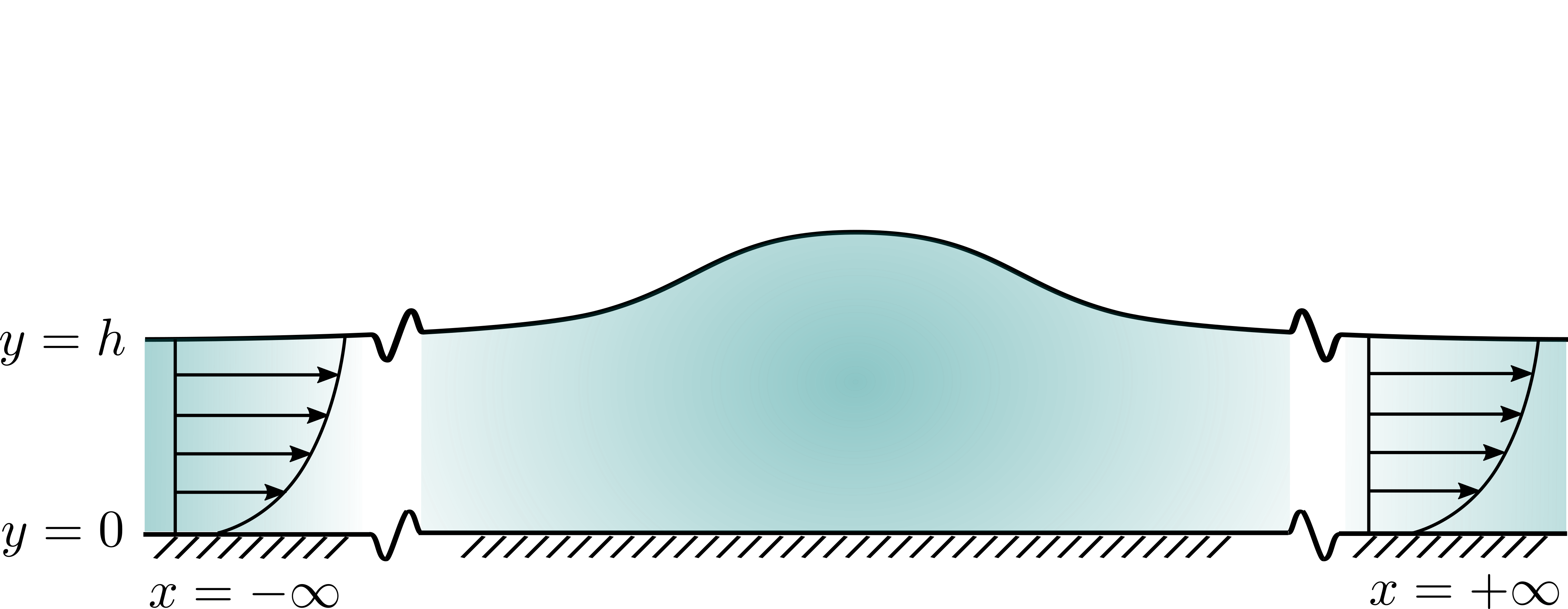
Figure 2: A sketch of the solitary wave profile on a unidirectional flow.

Now we are in a position to formulate our main result about the existence of solitary waves of elevation.

Theorem 1.

For every sufficiently large $b>0$ problem (1a)–(1d), (2) has a solution $(\psi,\eta)$ with the following properties:

(i) $\eta(X)>h$ for all $X\in\mathbb{R}$, that is, $\eta$ describes a solitary wave of elevation;

(ii) there are two stagnation points on the bottom and two streamlines within the fluid domain connect these points (see Figure 1); the critical level corresponds to the lower streamline, whereas the upper one of these streamlines is critical;

(iii) all streamlines below the critical one are closed and surround an interior stagnation point on the vertical line through the crest;

(iv) all streamlines above the critical one are diffeomorphic to the free surface profile.

An equivalent formulation of this assertion and its proof are given in the next two sections. Our approach is based on a carefully chosen scaling of the original problem. Then we apply the spatial dynamics method to the scaled problem in the same way as in Kozlov & Lokharu (2019). This allows us to reduce the problem to a finite-dimensional Hamiltonian system; it has one degree of freedom and admits a homoclinic orbit describing a solitary wave of elevation in the original coordinates. The orbit goes around an equilibrium point representing a shear flow of constant depth with a counter-current and this guarantees the presence of a stagnation point and a critical streamline as is illustrated in Figure 1 above.

2 Reformulation of the problem

To avoid difficulties arising from the fact that $b$ is large, it is convenient to scale variables as follows:

$$\bar{x}=\sqrt{b}X,\ \ \bar{y}=\sqrt{b}Y,\ \ \bar{\eta}(\bar{x})=\sqrt{b}\,\eta(X),\ \ \bar{\psi}(\bar{x},\bar{y})=\psi(X,Y).$$

This transforms (1a)–(1d) into

$$\bar{\psi}_{\bar{x}\bar{x}}+\bar{\psi}_{\bar{y}\bar{y}}-1 =0 \text{for }0<\bar{y}<\bar{\eta}(\bar{x}),$$ (3a)

$$\bar{\psi}(\bar{x},\bar{y}) =0 \text{on }\bar{y}=0,$$ (3b)

$$\bar{\psi}(\bar{x},\bar{y}) =1 \text{on }\bar{y}=\bar{\eta},$$ (3c)

$$|\nabla\bar{\psi}|^{2}+2\gamma\bar{y} =\bar{R} \text{on }\bar{y}=\bar{\eta},$$ (3d)

where $\gamma=b^{-3/2}$ and $\bar{R}=Rb^{-1}$. This problem describes two-dimensional waves with vorticity (the latter is equal to one) and weak gravity because $\gamma$ is a small parameter provided $b$ is large.

Let us consider the stream solution $\bar{\psi}=u(\bar{y};s)$ and $\bar{\eta}=h(s)$ such that $u^{\prime}(0)=s$. From (3a)–(3c) one obtains the unique pair

$$u(\bar{y};s)=\tfrac{1}{2}\bar{y}^{2}+s\bar{y},\ \ h(s)=-s+\sqrt{2+s^{2}}\,,$$ (4)

and (3d) yields the corresponding Bernoulli constant:

$$\bar{R}(s)=2\gamma h(s)+[u^{\prime}(h(s);s)]^{2}.$$

If $s<0$, then the laminar flow defined by (4) has a counter-current, whereas the corresponding flow is unidirectional when $s>0$. In what follows we assume that $s<0$.

2.1 Flattening transformation

Changing the coordinates $(\bar{x},\bar{y})$ to

$$(x,y)=\left(\bar{x},\frac{\bar{y}}{\bar{\eta}(\bar{x})}h(s)\right),$$

we map the water domain onto the strip $\mathbb{R}\times(0,h(s))$. Let

$$\hat{\Phi}(x,y)=\bar{\psi}\left(\bar{x},\bar{y}\right)$$

be new unknown function, for which problem (3) with $\bar{R}=\bar{R}(s)$ takes the form:

$$\Big{[}\hat{\Phi}_{x}-\frac{y\bar{\eta}_{x}}{\bar{\eta}}\hat{\Phi}_{y}\Big{]}_{x}-\frac{y\bar{\eta}_{x}}{\bar{\eta}}\Big{[}\hat{\Phi}_{x}-\frac{y\bar{\eta}_{x}}{\bar{\eta}}\hat{\Phi}_{y}\Big{]}_{y}+\frac{h^{2}(s)}{\bar{\eta}^{2}}\hat{\Phi}_{yy}-1 =0 \text{for }0<y<h(s),$$ (5a)

$$\hat{\Phi}(x,0) =0 \text{for }x\in\mathbb{R},$$ (5b)

$$\hat{\Phi}(x,h(s)) =1 \text{for }x\in\mathbb{R},$$ (5c)

$$\hat{\Phi}_{y}^{2}(x,h(s))-\frac{\bar{\eta}^{2}(\bar{R}(s)-2\gamma\bar{\eta})}{h(s)^{2}(1+\bar{\eta}_{x}^{2})} =0 \text{for }x\in\mathbb{R}.$$ (5d)

Note that $\hat{\Phi}=u(y;s)$ and $\bar{\eta}=h(s)$ is a solution of this system. Let us write (5) as a first-order system, for which purpose it is convenient to introduce the variable $\hat{\Psi}$ conjugate to $\hat{\Phi}$ (cf. Kozlov & Kuznetsov (2013)):

$$\hat{\Psi}(x,y)=\frac{\bar{\eta}}{h(s)}\Big{[}\hat{\Phi}_{x}-\frac{y\bar{\eta}_{x}}{\bar{\eta}}\hat{\Phi}_{y}\Big{]}.$$ (6)

This allows us to write (5) as follows:

$$\hat{\Phi}_{x}=\frac{h(s)}{\bar{\eta}}\hat{\Psi}+\frac{y}{\bar{\eta}}\bar{\eta}_{x}\hat{\Phi}_{y} \text{for }(x,y)\in\mathbb{R}\times(0,h(s)),$$ (7a)

$$\hat{\Psi}_{x}=\frac{\bar{\eta}_{x}}{\bar{\eta}}(y\hat{\Psi})_{y}-\frac{h(s)}{\bar{\eta}}\hat{\Phi}_{yy}+\frac{\bar{\eta}}{h(s)} \text{for }(x,y)\in\mathbb{R}\times(0,h(s)),$$ (7b)

$$\hat{\Phi}(x,0)=\hat{\Psi}(x,0)=0 \text{for }x\in\mathbb{R},$$ (7c)

$$\hat{\Phi}(x,y)=1 \text{on }y=h(s),$$ (7d)

$$\hat{\Phi}_{y}^{2}+\hat{\Psi}^{2}=\frac{\bar{\eta}^{2}}{h^{2}(s)}(\bar{R}(s)-2\gamma\bar{\eta}) \text{on }y=h(s).$$ (7e)

Furthermore, we have that

$$\bar{\eta}_{x}(x)=-\frac{\hat{\Psi}(x,h(s))}{\hat{\Phi}_{y}(x,h(s))}$$ (8)

Relations (7) can be considered as an infinite-dimensional dynamical system for $\hat{\Phi}$ and $\hat{\Psi}$ only. Indeed, $\bar{\eta}$ and $\bar{\eta}_{x}$ can be eliminated with the help of (7e) and (8), which will be formalised in the next section.

2.2 Linearization around a laminar flow

Let us linearize relations (7) around the stream solution $\hat{\Phi}=u(y;s),\hat{\Psi}=0,\bar{\eta}=h(s)$, for which purpose we introduce

$$\Phi=\hat{\Phi}-u-\frac{yu_{y}}{h(s)}\zeta,\ \ \Psi=\hat{\Psi},\ \ \zeta=\bar{\eta}-h(s).$$

Then we obtain from (7):

$$\Phi_{x}=\Psi+N_{1} \text{for }(x,y)\in\mathbb{R}\times(0,h(s)),$$ (9a)

$$\Psi_{x}=-\Phi_{yy}+N_{2} \text{for }(x,y)\in\mathbb{R}\times(0,h(s)),$$ (9b)

$$\Phi(x,0)=\Psi(x,0)=0 \text{for }x\in\mathbb{R},$$ (9c)

$$\Phi_{y}-\kappa\Phi=N_{3} \text{on }y=h(s).$$ (9d)

Here

$$\kappa=\kappa(s,\gamma)=\frac{\gamma+k}{k^{2}}\ \mbox{and}\ k=k(s)=h(s)+s=\sqrt{2+s^{2}}>0\,,$$

whereas the nonlinear operators in (9a), (9b) and (9c) have the form

$$\begin{split}N_{1}&=\frac{-h(s)\Psi\zeta+y\zeta_{x}(y\zeta+h(s)\Phi_{y})}{h(s)(h(s)+\zeta)},\\ N_{2}&=\frac{\zeta^{2}+h(s)\zeta_{x}(y\Psi)_{y}+h(s)\zeta\Phi_{yy}}{h(s)(h(s)+\zeta)},\\ N_{3}&=\frac{-h(s)^{2}\Psi^{2}+(\zeta+\Phi_{y})(-h(s)\zeta(h(s)-2k)+2\zeta^{2}k-h(s)^{2}\Phi_{y})}{2(h(s)+\zeta)^{2}k},\end{split}$$

respectively. Moreover, we find that

$$\zeta(x)=-\frac{\Phi(x,h(s))}{k},\ \ \zeta_{x}(x)=-\frac{h(s)\Psi(x,h(s))}{h(s)\zeta+h(s)k+\zeta k+h(s)\Phi_{y}(x,h(s))}.$$ (10)

Substituting these expressions into formulae for $N_{1}$, $N_{2}$ and $N_{3}$, we see that (9a) and (9b) form an infinite-dimensional reversible dynamical system on the manifold defined by (9c) and (9d). The presence of the nonlinear boundary condition (9d) is inessential because it is reducible to a homogeneous one after a proper change of variables; see Groves & Wahlén (2008) and Kozlov & Lokharu (2019) for details.

Let us assume the following regularity

$$\Psi\in C(\mathbb{R};X_{1}),\ \ \Phi\in C(\mathbb{R};X_{2}),$$

where

$$X_{m}=\{f\in H^{m}(0,1):\ f(0)=0\},\ \ \ m=0,1,2,$$

and $H^{m}(0,1)$ denotes the Sobolev space. Furthermore, it is clear that $k$ and $\kappa$ depend analytically on $s$ and $\gamma$, provided their values are small, and so the same is true for the operators $N_{1}$, $N_{2}$ and $N_{3}$. More precisely, let

$$\Lambda_{\epsilon}=\{\lambda=(s,\gamma)\in\mathbb{R}^{2}:|s|^{2}+|\gamma|^{2}<\epsilon^{2}\}$$

be a small neighbourhood of the origin in the parameter space, then

$$N_{1}\in C^{\infty}(X_{1}\times X_{2}\times\Lambda_{\epsilon};H^{1}(0,1)),\quad N_{2}\in C^{\infty}(X_{1}\times X_{2}\times\Lambda_{\epsilon};L^{2}(0,1)),$$

whereas $N_{3}\in C^{\infty}(X_{1}\times X_{2}\times\Lambda_{\epsilon};\mathbb{R})$. Moreover, all derivatives of these operators are bounded and uniformly continuous in $\Lambda_{\epsilon}$.

2.3 A linear eigenvalue problem

The centre subspace of (9) is determined by the imaginary spectrum of the linear operator $L(\Psi,\Phi)=(-\Phi_{YY},\Psi)$ defined on a subspace of $X_{1}\times X_{2}$ and subject to the homogeneous condition

$$\Phi_{Y}(h(s))=\kappa\Phi(h(s)).$$

It is straightforward to find that the spectrum is discrete and consists of all $\hat{\tau}\in{\mathbb{C}}$ such that $\mu=\hat{\tau}^{2}$ is an eigenvalue of the following Sturm–Liouville problem:

$$-\varphi_{YY}=\mu\varphi\ \mbox{on}\ (0,1);\quad\varphi(0)=0\ \mbox{and}\ [\varphi_{Y}-\kappa\varphi]_{Y=1}=0\,.$$ (11)

(Basic facts about Sturm–Liouville problems can be found in Teschl (2012).) Thus, the imaginary part of the spectrum of $L$ corresponds to the negative eigenvalues of (11).

The spectrum of (11) is discrete and consists of real simple eigenvalues say

$$\mu_{1}<\mu_{2}<\cdots<\mu_{j}<\cdots$$

accumulating at infinity, and the corresponding eigenfunctions $\varphi_{j}$ can be rescaled to form an orthonormal basis for $L^{2}(0,h(s))$.

2.4 On the existence of a negative eigenvalue

Let us investigate the spectral problem (11) for small negative $s$ and small positive $\gamma$. Solving (11) explicitly, we find that the unique negative eigenvalue $\mu_{1}=-\tau^{2}$ satisfies the dispersion equation:

$$\tau h(s)\coth(\tau h(s))=\kappa h(s).$$

Using the definition of $\kappa$, we obtain that

$$\kappa h(s)=1+\frac{\gamma-s}{\sqrt{2}}+O(\epsilon^{2})\ \ \mbox{as}\ \epsilon\to 0.$$

Thus, $\kappa h(s)>1$ for all sufficiently small negative $s$ and small $\gamma>0$, and so the dispersion equation has a unique root $\tau>0$ such that

$$[\tau h(s)]^{2}=3\frac{\gamma-s}{\sqrt{2}}+O(\epsilon^{2})\ \ \mbox{as}\ \epsilon\to 0.$$ (12)

Since $h(s)=\sqrt{2}+O(s)$, we have the following approximate expression for the normalized eigenfunction $\phi_{1}$:

$$\phi_{1}(y)=c_{0}\,y(1+O(\epsilon))\ \ \mbox{as}\ \epsilon\to 0,\ \mbox{where}\ c_{0}=\sqrt{\frac{3}{2^{3/2}}}\,.$$ (13)

It is uniform with respect to $y\in[0,h(s)]$ and $\lambda=(s,\gamma)\in\Lambda_{\epsilon}$.

Finally, it is worth mentioning that the positive part of the spectrum of $L$ is separated from zero, because $\mu_{2}>\pi^{2}/h^{2}(s)>\pi^{2}/2$.

3 Reduction to a finite-dimensional system

Let us reduce (9) to a finite-dimensional Hamiltonian system by using the centre-manifold technique developed by Mielke (1988), who considered quasilinear elliptic problems in cylinders. For this purpose we apply a result obtained in Kozlov & Lokharu (2019) (namely, Theorem 3.1), which is a convenient way to obtain a reduced problem. Prior to that we use the so-called spectral splitting to decompose the system.

3.1 Spectral decomposition and reduction

Following the method proposed in Kozlov & Lokharu (2019), we seek $(\Phi,\Psi)$ in the form

$$\Phi(x,y)=\alpha(x)\,\varphi_{1}(y)+\widetilde{\Phi}(x,y),\quad\Psi(x,y)=\beta(x)\,\varphi_{1}(y)+\widetilde{\Psi}(x,y)\,,$$

where $\widetilde{\Phi}$ and $\widetilde{\Psi}$ are orthogonal to $\varphi_{1}$ in $L^{2}(0,h(s))$; that is,

$$\alpha(x)=\int_{0}^{h(s)}\Phi(x,y)\,\varphi_{1}(y)\,\mathrm{d}\kern 0.2pty,\quad\beta(x)=\int_{0}^{h(s)}\Psi(x,y)\,\varphi_{1}(y)\,\mathrm{d}\kern 0.2pty\,.$$

For $\lambda\in\Lambda_{\epsilon}$ we define projectors ${\mathcal{P}}_{\lambda}\phi=\alpha\varphi_{1}$ and $\widetilde{\mathcal{P}}_{\lambda}={\rm id}-{\mathcal{P}}$, which are well defined on $H^{1}(0,h(s))$ and orthogonal in $L^{2}(0,h(s))$. Multiplying (9a) and (9b) by $\varphi_{1}$ and integrating over $(0,h(s))$, we obtain

$$\alpha_{X}=\beta+F_{1}(\Psi,\Phi;\lambda),$$ (14)

$$\beta_{X}=-\tau^{2}\alpha+F_{2}(\Psi,\Phi;\lambda),$$ (15)

where

$$\begin{split}&F_{1}(\Psi,\Phi;\lambda)=\int_{0}^{h(s)}N_{1}(\Psi,\Phi;\lambda)\varphi_{1}\,\mathrm{d}\kern 0.2pty,\\ &F_{2}(\Psi,\Phi;\lambda)=\int_{0}^{h(s)}N_{2}(\Psi,\Phi;\lambda)\varphi_{1}\,\mathrm{d}\kern 0.2pty-N_{3}(\Psi,\Phi;\lambda)\,\varphi_{1}(h(s))\,.\end{split}these$$

The system for $\widetilde{\Phi}$ and $\widetilde{\Psi}$ is as follows:

$$\widetilde{\Phi}_{x}=\widetilde{\Psi}+\widetilde{\mathcal{P}}_{\lambda}(N_{1}),$$ (16)

$$\widetilde{\Psi}_{x}=-\widetilde{\Phi}_{yy}+\widetilde{\mathcal{P}}_{\lambda}(N_{2})+\varphi_{1}(h(s))\,\varphi_{1}N_{3},$$ (17)

and these functions satisfy the following boundary conditions:

$$\widetilde{\Phi}(x,0)=\widetilde{\Psi}(x,0)=0,\quad\widetilde{\Phi}_{Y}(x,h(s))-\kappa\,\widetilde{\Phi}(x,h(s))=N_{3}\,.$$ (18)

Moreover, let $\widetilde{X}_{j}^{(\lambda)}$ denote $\widetilde{\mathcal{P}}_{\lambda}(X_{j})$, $j=0,1,2$, where $\lambda\in\Lambda_{\epsilon}$, then for all $x\in\mathbb{R}$ and $\lambda\in\Lambda_{\epsilon}$ we have that $\widetilde{\Psi}\in\widetilde{X}_{1}^{(\lambda)}$ and $\widetilde{\Phi}\in\widetilde{X}_{2}^{(\lambda)}$.

Applying Theorem 3.1 proved in Kozlov & Lokharu (2019) to the decomposed system (14)–(18), we arrive at the following assertion.

Theorem 2.

For any $m\geq 2$ there exist $\epsilon>0$, neighbourhoods $W\subset\mathbb{R}^{2},$ $W_{1}\subset X_{1},W_{2}\subset X_{2}$ and the vector-functions $r_{j}:W\times\Lambda_{\epsilon}\to W_{j},$ $j=1,2,$ of the class $C^{m}(W\times\Lambda_{\epsilon})$ with the following properties.

• The derivatives of $r_{1}$ and $r_{2}$ are bounded and uniformly continuous, and the estimate

  $$\|r_{1};H^{1}\|+\|r_{2};H^{2}\|=O(|\alpha|^{2}+|\beta|^{2}),\ \ where\ (\alpha,\beta)\in W,$$

  holds uniformly with respect to $\lambda\in\Lambda_{\epsilon}$.

• $r_{j}(\alpha,\beta,\lambda)\in\widetilde{X}_{j}^{(\lambda)},$ $j=1,2,$ for all $\lambda\in\Lambda_{\epsilon}$ and all $(\alpha,\beta)\in W$.

• The set

  $$M^{\lambda}=\{(\Psi^{r}[\alpha,\beta;\lambda],\Phi^{r}[\alpha,\beta;\lambda])\,:\,(\alpha,\beta)\in W,\ \lambda\in\Lambda_{\epsilon}\}\subset X_{1}\times X_{2},$$

  where $\Psi^{r}[\alpha,\beta;\lambda]=\beta\varphi_{1}+r_{1}(\alpha,\beta;\lambda)$ and $\Phi^{r}[\alpha,\beta;\lambda]=\alpha\varphi_{1}+r_{2}(\alpha,\beta;\lambda),$ is a locally invariant manifold for (9); that is, a unique solution of (9) goes through every point of $M^{\lambda}$ and this solution belongs to $M^{\lambda}$ as long as $(r_{1},r_{2})\in W_{1}\times W_{2}$.

• Every global solution $(\alpha,\beta)\in C(\mathbb{R};W)$ of the reduced system

  $$\begin{split}&\alpha_{x}=\beta+F_{1}(\Psi^{r}[\alpha,\beta;\lambda],\Phi^{r}[\alpha,\beta;\lambda];\lambda),\\ &\beta_{x}=\mu_{1}\alpha+F_{2}(\Psi^{r}[\alpha,\beta;\lambda],\Phi^{r}[\alpha,\beta;\lambda];\lambda),\end{split}$$ (19)

  where $\lambda\in\Lambda_{\epsilon},$ generates the solution $(\Psi,\Phi)$ of (9) with

  $$\Psi(x,y)=\Psi^{r}[\alpha(x),\beta(x);\lambda](y),\ \ \Phi(x,y)=\Phi^{r}[\alpha(x),\beta(x);\lambda](y).$$

  Moreover, the reduced system (19) is reversible.

A direct calculation shows that the reduced system (19) has the following structure:

$$\begin{split}&\alpha_{x}=\beta[1+O(|\alpha|+|\beta|^{2})],\\ &\beta_{x}=-\tau^{2}\alpha+A\alpha^{2}+O(|\alpha|^{3}+|\beta|^{2}),\end{split}$$ (20)

where $A=\tfrac{1}{2}c_{0}^{3}+O(\epsilon)$ and $c_{0}$ is defined in (13). Now we are in a position to formulate and prove the following.

Theorem 3.

Problem (20) has a homoclinic solution such that

$$\alpha_{h}(x)=\tau^{2}\alpha^{\star}_{+}-\left(\tfrac{3}{2}\alpha_{+}^{\star}\tau^{2}+O(\tau^{4})\right)\operatorname{sech}^{2}(\tau x/2)\ \ as\ \tau\to 0,$$ (21)

whereas $\beta_{h}$ is defined implicitly by the first formula (20). Here $\alpha^{\star}_{+}=1/A+O(\tau^{2})$ is a constant independent of $x$.

Proof.

It is known (see Groves & Stylianou (2014),Kozlov & Kuznetsov (2013)) that problem (1a)–(1d) has a Hamiltonian structure (even for arbitrary vorticity) with the role of time played by the horizontal coordinate. The Hamiltonian is the flow force invariant which has the following form in the original coordinates $(X,Y)$:

$${\mathcal{S}}=\left[\tfrac{1}{2}R-b\right]\eta(X)-\tfrac{1}{2}\Big{\{}\eta^{2}(X)-\int_{0}^{\eta(X)}\tfrac{1}{2}(\psi_{Y}^{2}-\psi_{X}^{2})+b\psi\,\mathrm{d}\kern 0.2ptY\Big{\}}.$$

Thus, the reduced system (20) has a constant of motion ${\mathcal{H}}(\alpha,\beta)$, to obtain which one has to subject $b^{-1}{\mathcal{S}}$ to all changes of variables described above. A direct calculation yields that

$$\mathcal{H}(\alpha,\beta)=\frac{1}{2}(\beta^{2}+\tau^{2}\alpha^{2})-\frac{A}{3}\alpha^{3}+O\left(\alpha^{4}+\beta^{2}\right)(=b^{-1}S),$$

where $A$ is the coefficient in the second equation (20). It should be noted that $\mathcal{H}(\alpha,\beta)$ is an even function of $\beta$ which follows from reversibility of this system. The form of $\mathcal{H}(\alpha,\beta)$ suggests that variables must be scaled as follows:

$$\alpha(x)=\tau^{2}\alpha_{1}(x_{1}),\ \ \beta(x)=\tau^{3}\beta_{1}(x_{1}),\ \ x=\tau^{-1}x_{1},\ \ {\mathcal{H}}(\alpha,\beta)=\tau^{6}{\mathcal{H}}_{1}(\alpha_{1},\beta_{1}),$$

where

$${\mathcal{H}}_{1}(\alpha_{1},\beta_{1})=\frac{1}{2}(\alpha_{1}^{2}+\beta_{1}^{2})-\frac{A}{3}\alpha_{1}^{3}+\tau^{2}O(|\alpha^{3}_{1}|+|\beta^{4}_{1}|),$$

and so the scaled equations are

$$\begin{split}&[\alpha_{1}]_{x_{1}}=\beta_{1}+\tau^{2}\beta_{1}O(|\alpha_{1}|+|\beta_{1}|^{2}),\\ &[\beta_{1}]_{x_{1}}=-\alpha_{1}+A\alpha_{1}^{2}+\tau^{2}O(|\alpha_{1}|^{3}+|\beta_{1}|^{2}).\end{split}$$ (22)

(a) Graph of the function ${\mathcal{H}}_{1}(\alpha_{1},0)$

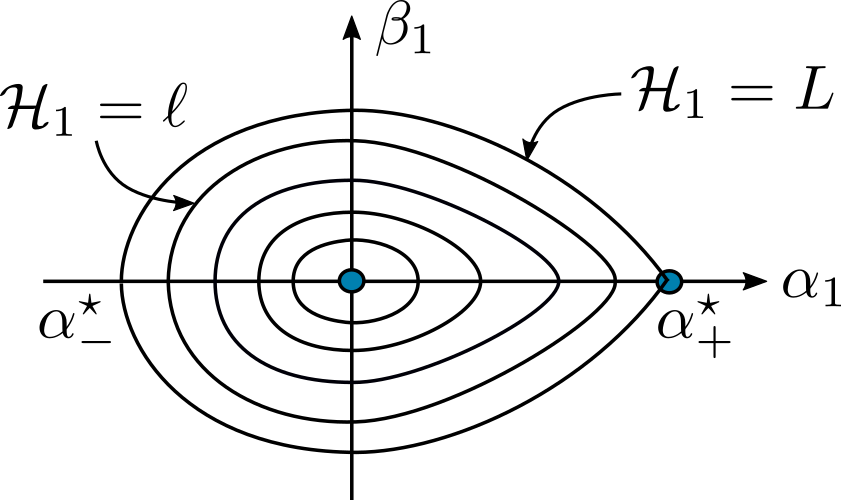
(b) Phase portrait

Figure 3: The behaviour of the Hamiltonian near the origin (A) and its level curves (B)

The graph of ${\mathcal{H}}_{1}(\alpha,0)$ in a neighbourhood of the origin is sketched in Figure 3A. It is clear that the local maximum of this function close to the origin is attained at $\alpha=\alpha^{\star}_{+}$ and $L={\mathcal{H}}_{1}(\alpha^{\star}_{+},0)$ is its value. Then the level line

$${\mathcal{H}}_{1}(\alpha_{1},\beta_{1})=\ell$$

is a closed curve for every $\ell\in(0,L)$ and it corresponds to a periodic solution. The contour

$${\mathcal{H}}_{1}(\alpha_{1},\beta_{1})=L$$

defines the homoclinic orbit; see a sketch of level lines in Figure 3B. The values $\alpha_{-}^{\star}$ and $\alpha_{+}^{\star}$ correspond to the “crest” and the limiting depth respectively. An essential feature of the homoclinic orbit is that $\alpha_{1}$ attains negative values on its left part; this implies that there is a stagnation point as will be shown below.

Let us turn to proving (21). By $\alpha_{1}^{h}$ we denote a homoclinic solution to (22). It is easy to see that it is monotone on each side of the crest; the latter corresponds to the value $\alpha_{1}^{h}(0)=\alpha_{-}^{\star}$. Then we have

$$X_{1}=\int_{0}^{x_{1}}\textrm{d}x_{1}=\int_{\alpha_{-}^{\star}}^{\alpha_{1}^{h}(x_{1})}\frac{\mathrm{d}\kern 0.2pt\alpha_{1}}{[\alpha_{1}^{h}]_{x_{1}}},$$

where $[\alpha_{1}^{h}]_{x_{1}}=\beta_{1}^{h}[1+O(\tau^{2})]$; see the first equation (22). On the other hand,

$$L-{\mathcal{H}}_{1}(\alpha_{1}^{h},0)=\frac{[\beta_{1}^{h}]^{2}}{2}\big{\{}1+\tau^{2}O([\beta_{1}^{h}]^{2})\big{\}},$$

where the system’s reversibility is used. Expressing $[\beta_{1}^{h}]^{2}$ from the last formula and taking into account the fact it is positive on the interval of the integration, we obtain

$$x_{1}=\int_{\alpha_{-}^{\star}}^{\alpha_{1}^{h}(x_{1})}\frac{\mathrm{d}\kern 0.2pt\alpha_{1}}{[\alpha_{1}^{h}]_{x_{1}}}=[1+O(\tau^{2})]\int_{\alpha_{-}^{\star}}^{\alpha_{1}^{h}(x_{1})}\frac{\mathrm{d}\kern 0.2pt\alpha_{1}}{\sqrt{2[L-{\mathcal{H}}_{1}(\alpha_{1}^{h},0)]}}.$$ (23)

Let us find an approximation of the integral using a third degree polynomial for the expression under the square root; more precisely, let us show that

$$\begin{split}L-{\mathcal{H}}_{1}(\alpha_{1},0)=a(\tau)(\alpha_{1}-\alpha_{-}^{\star})(\alpha_{1}-\alpha_{+}^{\star})^{2}+\tau^{2}O(|\alpha_{1}-\alpha_{-}^{\star}||\alpha_{1}-\alpha_{+}^{\star}|^{2}),\end{split}$$ (24)

where

$$a(\tau)=-\frac{L}{\alpha_{-}^{\star}[\alpha_{+}^{\star}]^{2}}=\frac{A}{3}+O(\tau^{2}).$$

It should be emphasised that (24) is used as a representation of $L-{\mathcal{H}}_{1}(\alpha_{1},0)$ only on the interval $[\alpha_{-}^{\star},\alpha_{+}^{\star}]$. To prove (24) we note that

$$L-{\mathcal{H}}_{1}(\alpha_{1},0)=L-\frac{\alpha_{1}^{2}}{2}+A\frac{\alpha_{1}^{3}}{3}+\tau^{2}O(|\alpha_{1}|^{3})=:Q_{1}(\alpha_{1})+\tau^{2}O(|\alpha_{1}|^{3}).$$

A direct calculation yields that the estimate $O(\tau^{2})$ holds for

$$Q_{1}(\alpha_{-}^{\star}),\ Q_{1}(\alpha_{+}^{\star}),\ \partial_{\alpha_{1}}Q_{1}(\alpha_{+}^{\star})$$

Therefore, solving a linear system, one obtains that up to $O(\tau^{2})$ the coefficients of

$$a(\tau)(\alpha_{1}-\alpha_{-}^{\star})(\alpha_{1}-\alpha_{+}^{\star})^{2}$$

are the same as those of $Q_{1}$. This shows that the error in (24) has the same estimate $O(\tau^{2})$. It remains to use the fact that $L-{\mathcal{H}}_{1}(\alpha_{1},0)$ has a simple zero at $\alpha_{-}^{\star}$ and a double zero at $\alpha_{+}^{\star}$ which proves (24).

Now we have

$$\begin{split}\int_{\alpha_{-}^{\star}}^{\alpha_{1}^{h}(x_{1})}\frac{\mathrm{d}\kern 0.2pt\alpha_{1}}{\sqrt{2(L-{\mathcal{H}}_{1}(\alpha_{1},0))}}\!=&[1+O(\tau^{2})]\int_{\alpha_{-}^{\star}}^{\alpha_{1}^{h}(x_{1})}\frac{\mathrm{d}\kern 0.2pt\alpha_{1}}{\sqrt{2a(\alpha_{1}-\alpha_{-}^{\star})(\alpha_{1}-\alpha_{+}^{\star})^{2}}}\\ =&\frac{1+O(\tau^{2})}{a_{0}\sqrt{2a}}\left[\ln\left|\frac{a_{0}+\sqrt{\alpha_{1}-\alpha_{-}^{\star}}}{a_{0}-\sqrt{\alpha_{1}-\alpha_{-}^{\star}}}\right|\right]_{\alpha_{1}=\alpha_{-}^{\star}}^{\alpha_{1}=\alpha_{1}^{h}(x_{1})}\\ =&\frac{1+O(\tau^{2})}{a_{0}\sqrt{2a}}\left(\ln\left[\frac{\left(a_{0}+\sqrt{\alpha_{1}^{h}(x_{1})-\alpha_{-}^{\star}}\right)^{2}}{\alpha_{+}^{\star}-\alpha_{1}^{h}(x_{1})}\right]\right),\end{split}$$

where $a_{0}=\sqrt{\alpha_{+}^{\star}-\alpha_{-}^{\star}}$. Comparing this and (23), one obtains the following formula for the solitary wave solution:

$$\alpha_{1}^{h}(x_{1})=\alpha_{+}^{\star}-\left[\frac{6}{A}+O(\tau^{2})\right]e^{-(1+O(\tau^{2}))x_{1}},$$ (25)

where formulas $\alpha_{-}^{\star}=-\alpha_{+}^{\star}/2+O(\tau^{2})$ and $\alpha_{+}^{\star}=1/A+O(\tau^{2})$ are taken into account. Furthermore, it is straightforward to show that

$$\|\alpha_{1}^{h}-\alpha_{1}^{h,\star}\|_{L^{\infty}(\mathbb{R})}=O(\tau^{2}),$$

where

$$\alpha_{1}^{h,\star}(x_{1})=\frac{1}{A}-\frac{3}{2A}\operatorname{sech}^{2}(x_{1}/2).$$

The latter is a homoclinic solution of (22) with $\tau=0$, in which case $\beta_{1}=[\alpha_{1}^{h,\star}]_{x_{1}}$. Combining this and the asymptotic formula (25), one arrives at (21) by rescaling variables to the original ones. ∎

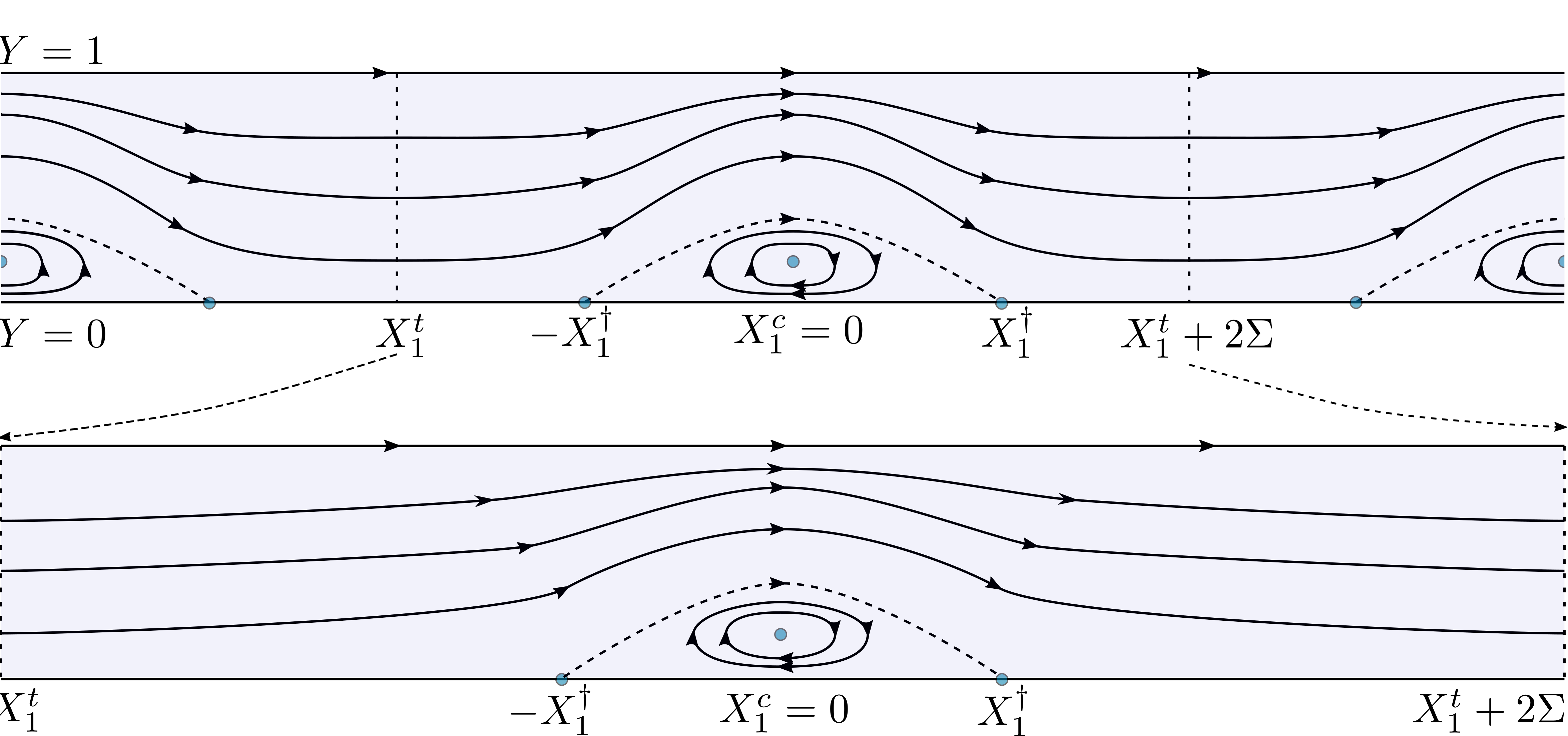
Figure 4: Two Stokes waves corresponding to different values of $\ell$ plotted in $(X_{1},Y)$-variables.

3.2 Periodic waves

An approximation of solutions for periodic waves can be found in the same way as for solitary waves. Indeed, let us consider the periodic solution $\alpha_{1}^{\ell}$ corresponding to some energy ${\mathcal{H}}_{1}=\ell$. Let the trough of the corresponding wave be located at $x_{1}^{c}=0$ and let the nearest crest to the left have the coordinate $x_{1}^{t}<x_{1}^{c}$ (see Figure 4). Then for every $x_{1}\in(x_{1}^{t}x_{1}^{c}]$ we have

$$x_{1}-x_{1}^{t}=\int_{\alpha_{-}}^{\alpha_{1}^{\ell}(x_{1})}\!\!\frac{\mathrm{d}\kern 0.2pt\alpha_{1}}{[\alpha_{1}^{\ell}]_{x_{1}}}=[1+O(\tau^{2})]\int_{\alpha_{-}}^{\alpha_{1}^{\ell}(x_{1})}\frac{\mathrm{d}\kern 0.2pt\alpha_{1}}{\sqrt{2[\ell-{\mathcal{H}}_{1}(\alpha_{1},0)]}}\,.$$ (26)

In particular, the half-period of this solution is equal to

$$\Sigma_{\ell}=x_{1}^{c}-x_{1}^{t}=[1+O(\tau^{2})]\int_{\alpha_{-}}^{\alpha_{+}}\!\!\frac{\mathrm{d}\kern 0.2pt\alpha_{1}}{\sqrt{2[\ell-{\mathcal{H}}_{1}(\alpha_{1},0)]}}\,,$$ (27)

and so $\Sigma_{\ell}\to+\infty$ as $\ell\to L$. Let us estimate the bottom width of a cat’s-eye vortex (in Figure 4, it is bounded above by the dashed streamline). On every interval symmetric about the crest and having the length $2\Sigma_{\ell}$, there are exactly two stagnation points on the bottom that bound the bottom-attached vortex (these points are shown solid in Figure 4), and $\alpha_{1}^{\ell}(\pm x_{1}^{\dagger})=0$ at these points nearest to the origin. From (26) the approximate formula follows:

$$-x_{1}^{\dagger}-x_{1}^{t}=[1+O(\tau^{2})]\int_{\alpha_{-}}^{0}\!\!\frac{\mathrm{d}\kern 0.2pt\alpha_{1}}{\sqrt{2[\ell-{\mathcal{H}}_{1}(\alpha_{1},0)]}}\,,$$

which yields that $x_{1}^{\dagger}=O(1)$ as $\ell\to L$ in view that the integral

$$\int_{\alpha_{-}}^{0}\!\!\frac{\mathrm{d}\kern 0.2pt\alpha_{1}}{\sqrt{2[L-{\mathcal{H}}_{1}(\alpha_{1},0)]}}$$

is finite. Indeed, the function $L-{\mathcal{H}}_{1}(\alpha_{1},0)$ has only one simple zero $\alpha_{1}=\alpha_{-}^{\star}$ on the interval of integration. Thus, $x_{1}^{\dagger}$ remains bounded when the wavelength goes to infinity, and the same is true for the domain occupied by cat’s-eye vortex. Therefore, the structure of streamlines is similar for the limiting solitary wave as shown in Figure 2.

4 Proof of Theorem 1

It is straightforward to recover the free surface profile which takes the form

$$\eta(X)=h_{-}+\sqrt{b}\left[\frac{3}{c_{0}^{2}}+O(\tau^{2})\right]\tau^{2}\textrm{sech}^{2}(\sqrt{b}\tau X/2)$$ (28)

in the original coordinates. Here $c_{0}^{2}=2Ak/\varphi_{1}(h(s))$ and $h_{-}$ is the depth of the unidirectional laminar flow conjugate to $b^{-1/2}h(s)$. Thus, $\eta(X)$ descibes a solitary wave of positive elevation.

To show that the flow, on which this wave propagates, has a bottom-attached cat’s-eye vortex, let us track back the changes of coordinates made above and find that

$$\hat{\Phi}_{y}=u_{y}+\Phi_{y}-(u_{y}+y)\Phi(x,h)/(kh).$$

Here $\Phi(x,y)=\alpha(x)\phi_{1}(y)+yO(\tau^{4})=c_{0}y\alpha(x)+yO(\tau^{4})$, and so

$$\hat{\Phi}_{y}=u_{y}\left[1-\frac{c_{0}}{k}\alpha(x)+O(\epsilon)+O(y)\right]+\alpha(X)(c_{0}+O(y)).$$

Since $s<0$, formula (4) implies that $u_{y}<0$ near the bottom, whereas the expression in the square brackets is positive. Moreover, it was established in the proof of Theorem 3 that the function $\alpha(x)$ attains negative values for some $x$. Taking this into account, the last formula shows that $\hat{\Phi}_{y}$ attains negative values near the bottom. More careful but simple analysis yields that the set of streamlines of $\hat{\Phi}$ has the structure shown in Figure 1 and it is essentially the same for $\psi$.

Acknowledgements. V. K. was supported by the Swedish Research Council (VR), 2017-03837. N. K. acknowledges the support from the Linköping University.

References

- Aasen & Varholm (2017) Aasen, Ailo & Varholm, Kristoffer 2017 Traveling gravity water waves with critical layers. Journal of Mathematical Fluid Mechanics 20 (1), 161–187.
- Amick et al. (1982) Amick, C. J., Fraenkel, L. E. & Toland, J. F. 1982 On the Stokes conjecture for the wave of extreme form. Acta Math. 148, 193–214.
- Amick & Toland (1981a) Amick, C. J. & Toland, J. F. 1981a On periodic water-waves and their convergence to solitary waves in the long-wave limit. Philos. Trans. Roy. Soc. London Ser. A 303 (1481), 633–669.
- Amick & Toland (1981b) Amick, C. J. & Toland, J. F. 1981b On solitary water-waves of finite amplitude. Arch. Rational Mech. Anal. 76 (1), 9–95.
- Benjamin (1962) Benjamin, T. B. 1962 The solitary wave on a stream with an arbitrary distribution of vorticity. J. Fluid Mech. 12, 97–116.
- Constantin & Strauss (2004) Constantin, Adrian & Strauss, Walter 2004 Exact steady periodic water waves with vorticity. Comm. Pure Appl. Math. 57 (4), 481–527.
- Constantin et al. (2016) Constantin, Adrian, Strauss, Walter & Vărvărucă, Eugen 2016 Global bifurcation of steady gravity water waves with critical layers. Acta Mathematica 217 (2), 195–262.
- Craig & Sternberg (1988) Craig, Walter & Sternberg, Peter 1988 Symmetry of solitary waves. Communications in Partial Differential Equations 13 (5), 603–633, arXiv: https://doi.org/10.1080/03605308808820554.
- Ehrnström et al. (2011) Ehrnström, Mats, Escher, Joachim & Wahlén, Erik 2011 Steady water waves with multiple critical layers. SIAM J. Math. Anal. 43 (3), 1436–1456.
- Friedrichs & Hyers (1954) Friedrichs, K. O. & Hyers, D. H. 1954 The existence of solitary waves. Comm. Pure Appl. Math. 7, 517–550.
- Groves & Nilsson (2018) Groves, M. D. & Nilsson, D. V. 2018 Spatial dynamics methods for solitary waves on a ferrofluid jet. Journal of Mathematical Fluid Mechanics .
- Groves & Stylianou (2014) Groves, Mark D. & Stylianou, Athanasios 2014 On the Hamiltonian structure of the planar steady water-wave problem with vorticity. C. R. Math. Acad. Sci. Paris 352 (3), 205–211.
- Groves & Wahlén (2007) Groves, M. D. & Wahlén, E. 2007 Spatial dynamics methods for solitary gravity-capillary water waves with an arbitrary distribution of vorticity. SIAM J. Math. Anal. 39 (3), 932–964.
- Groves & Wahlén (2008) Groves, M. D. & Wahlén, E. 2008 Small-amplitude Stokes and solitary gravity water waves with an arbitrary distribution of vorticity. Phys. D. 237 (10–12), 1530–1538.
- Hur (2008) Hur, Vera Mikyoung 2008 Exact solitary water waves with vorticity. Arch. Ration. Mech. Anal. 188 (2), 213–244.
- Keady & Norbury (1978) Keady, G. & Norbury, J. 1978 On the existence theory for irrotational water waves. Math. Proc. Cambridge Philos. Soc. 83 (1), 137–157.
- Kirchgässner (1982) Kirchgässner, Klaus 1982 Wave-solutions of reversible systems and applications. In Dynamical systems, II (Gainesville, Fla., 1981), pp. 181–200. New York: Academic Press.
- Kirchgässner (1988) Kirchgässner, K. 1988 Nonlinearly resonant surface waves and homoclinic bifurcation. In Advances in applied mechanics, Vol. 26, Adv. Appl. Mech., vol. 26, pp. 135–181. Boston, MA: Academic Press.
- Kozlov & Kuznetsov (2013) Kozlov, Vladimir & Kuznetsov, Nikolay 2013 Steady water waves with vorticity: spatial hamiltonian structure. Journal of Fluid Mechanics 733.
- Kozlov et al. (2015) Kozlov, V., Kuznetsov, N. & Lokharu, E. 2015 On bounds and non-existence in the problem of steady waves with vorticity. Journal of Fluid Mechanics 765, R1.
- Kozlov et al. (2017) Kozlov, V., Kuznetsov, N. & Lokharu, E. 2017 On the Benjamin–Lighthill conjecture for water waves with vorticity. Journal of Fluid Mechanics 825, 961–1001.
- Kozlov & Lokharu (2017) Kozlov, Vladimir & Lokharu, Evgeniy 2017 N-modal steady water waves with vorticity. Journal of Mathematical Fluid Mechanics 20 (2), 853–867.
- Kozlov & Lokharu (2019) Kozlov, V. & Lokharu, E. 2019 Small-amplitude steady water waves with critical layers: Non-symmetric waves. Journal of Differential Equations 267 (7), 4170–4191.
- Lavrentiev (1954) Lavrentiev, M. A. 1954 On the theory of long waves. Amer. Math. Soc. Transl. 102, 3–50.
- Majda & Bertozzi (2002) Majda, Andrew J. & Bertozzi, Andrea L. 2002 Vorticity and incompressible flow, Cambridge Texts in Applied Mathematics, vol. 27. Cambridge: Cambridge University Press.
- McLeod (1984) McLeod, J. B. 1984 The Froude number for solitary waves. Proceedings of the Royal Society of Edinburgh: Section A Mathematics 97, 193–197.
- Mielke (1986) Mielke, Alexander 1986 A reduction principle for nonautonomous systems in infinite-dimensional spaces. Journal of Differential Equations 65 (1), 68–88.
- Mielke (1988) Mielke, Alexander 1988 Reduction of quasilinear elliptic equations in cylindrical domains with applications. Math. Methods Appl. Sci. 10 (1), 51–66.
- Mielke (1991) Mielke, Alexander 1991 Hamiltonian and Lagrangian Flows on Center Manifolds. Springer Berlin Heidelberg.
- Ribeiro et al. (2017) Ribeiro, Roberto, Milewski, Paul A. & Nachbin, André 2017 Flow structure beneath rotational water waves with stagnation points. Journal of Fluid Mechanics 812, 792–814.
- Russell (1844) Russell, J. S. 1844 Report on waves. In Report of the fourteenth meeting of the British Association for the Advancement of Science, York, pp. 311–390. London: John Murray.
- Swan et al. (2001) Swan, C., Cummings, I.P. & James, R.L. 2001 An experimental study of two-dimensional surface water waves propagating on depth-varying currents. J. Fluid Mech 428, 273–304.
- Ter-Krikorov (1962) Ter-Krikorov, A.M. 1962 The solitary wave on the surface of a turbulent liquid. USSR Computational Mathematics and Mathematical Physics 1 (4), 1253–1264.
- Teschl (2012) Teschl, Gerald 2012 Ordinary differential equations and dynamical systems, Graduate Studies in Mathematics, vol. 140. American Mathematical Society, Providence, RI.
- Thomas (1981) Thomas, G. P. 1981 Wave-current interactions: an experimental and numerical study. part 1. linear waves. Journal of Fluid Mechanics 110, 457–474.
- Thomas Beale (1977) Thomas Beale, J. 1977 The existence of solitary water waves. Communications on Pure and Applied Mathematics 30 (4), 373–389, arXiv: https://onlinelibrary.wiley.com/doi/pdf/10.1002/cpa.3160300402.
- Vanden-Broeck (1994) Vanden-Broeck, J.-M. 1994 Steep solitary waves in water of finite depth with constant vorticity. Journal of Fluid Mechanics 274, 339–348.
- Vanden-Broeck (1995) Vanden-Broeck, J.-M. 1995 New families of steep solitary waves in water of finite depth with constant vorticity.
- Wahlén (2009) Wahlén, Erik 2009 Steady water waves with a critical layer. J. Differential Equations 246 (6), 2468–2483.
- Wheeler (2013) Wheeler, Miles H. 2013 Large-amplitude solitary water waves with vorticity. SIAM J. Math. Anal. 45 (5), 2937–2994.
- Wheeler (2015) Wheeler, Miles H. 2015 The Froude number for solitary water waves with vorticity. J. Fluid Mech. 768, 91–112.