Prompt $\eta_{c}$ meson production at the LHC in the NRQCD with $k_{T}$-factorization

Abstract

In the framework of the $k_{T}$-factorization approach, the prompt production of $\eta_{c}$ mesons at the LHC conditions is studied. Our consideration is based on the off-shell amplitudes for hard partonic subprocesses and on the nonrelativistic QCD (NRQCD) formalism for the formation of bound states. We try two latest parametrizations for noncollinear, or transverse momentum dependent (TMD) gluon densities derived from the Catani-Ciafaloni-Fiorani-Marchesini (CCFM) equation. We use the values of the nonperturbative matrix elements obtained from a combined fit of the $\eta_{c}$ and $J/\psi$ differential cross sections. Finally, we show an universal set of parameters that provides a reasonable simultaneous description for all of the available data on the prompt $J/\psi$ and $\eta_{c}$ production at the LHC.

I Motivation

Since long ago, the production of quarkonium states in high energy hadronic collisions remains an area of intense attention from both theoretical and experimental sides. Our present work continues the line started in the previous publications part1 ; part2 ; part3 . We have already considered there the production of $\psi^{\prime}$, $\chi_{c}$, and $J/\psi$ mesons and now come to $\eta_{c}$ mesons. As usual, we work in the $k_{T}$-factorization approach.

It is worth mentioning that the case of $\eta_{c}$ mesons turned out to be rather puzzling for conventional NRQCD calculations at next-to-leading order (NLO) Kniehl ; HanMa . This time, the theory was very unlucky to have too few free adjustable parameters. Having the nonperturbative matrix elements (NMEs) fixed from fitting all other production data, the theory lost its flexibility and made a prediction for $\eta_{c}$ by a huge factor off the measured cross section. The overall situation was even called ‘challenging’ Kniehl . The aim of the present note is to show that the approach used consistently in part1 ; part2 ; part3 meets no troubles with the $\eta_{c}$ data.

II Theoretical framework

As it was done previously for $\psi^{\prime}$, $\chi_{c}$ and $J/\psi$ production part1 ; part2 ; part3 , the present calculations are based on perturbative QCD and nonrelativistic bound state formalism (NRQCD). The production of $\eta_{c}$ mesons is dominated by the color singlet (CS) contribution that refers to the partonic subprocess

$$g^{*}(k_{1})+g^{*}(k_{2})\to\eta_{c}(p)$$ (1)

with the respective cross section

$$\sigma(pp\to\eta_{c}+X)$$

$$=\int\frac{2\pi}{x_{1}x_{2}s\,F}\,{{\cal F}}_{g}(x_{1},{\mbox{\bf k}}_{1T}^{2},\mu^{2})\,{{\cal F}}_{g}(x_{2},{\mbox{\bf k}}_{2T}^{2},\mu^{2})$$

$$\times\;\bigl{|}{\cal M}(g^{*}g^{*}\to\eta_{c})\bigr{|}^{2}\,d{\mbox{\bf k}}_{1T}^{2}\,d{\mbox{\bf k}}_{2T}^{2}\,dy_{\eta}\,\frac{d\phi_{1}}{2\pi}\,\frac{d\phi_{2}}{2\pi},$$ (2)

where ${k}_{1}$ and ${k}_{2}$ denote the initial gluon 4-momenta, $\phi_{1}$ and $\phi_{2}$ are the respective azimuthal angles, $y_{\eta}$ is the rapidity of $\eta_{c}$ meson, $x_{1}$ and $x_{2}$ are the gluon longitudinal momentum fractions, ${\cal M}(g^{*}g^{*}\to\eta_{c})$ is the hard scattering amplitude, and ${{\cal F}}_{g}(x_{i},{\mbox{\bf k}}_{iT}^{2},\mu^{2})$ is the transverse momentum dependent (TMD, or unintegrated) gluon density in a proton. In accordance with the general definition BycKaj , the off-shell gluon flux factor in (2) is taken as $F=2\lambda^{1/2}(\hat{s},k_{1}^{2},k_{2}^{2})$, where $\hat{s}=(k_{1}+k_{2})^{2}$.

In addition to the above, we have considered a number of color octet (CO) contributions and contribution from the feed-down $h_{c}\to\eta_{c}\,X$ process. The CO terms refer to the perturbative production of a color-octet $c\bar{c}^{[8]}$ pair followed by nonperturbative gluon radiation bringing the intermediate $c\bar{c}^{[8]}$ state to a real (colorless) meson:

$$g^{*}(k_{1})+g^{*}(k_{2})\to c\bar{c}^{[8]}\to\eta_{c}(p)+\mbox{soft~{}gluons}.$$ (3)

The intermediate color octet $c\bar{c}^{[8]}$ state can be either of ${}^{1}S_{0}$, ${}^{3}S_{1}$, ${}^{3}P_{0}$, ${}^{3}P_{1}$, ${}^{3}P_{2}$, or ${}^{1}P_{1}$, where we use standard spectroscopic notation. The probabilities of the subsequent nonperturbative soft transitions are not calculable within the theory and are usually accepted as free model parameters. There are, however, certain restrictions coming from some general principles. Whenever calculable or not, the nonperturbative amplitudes must be identical for transitions in both directions (i.e., from vectors to scalars and vice versa), as it is motivated by the heavy quark spin symmetry (HQSS). The amplitudes can only differ by an overall normalizing factor representing the averaging over spin degrees of freedom. Thus, we strictly have from this property Bodwin :

$$\left\langle{\cal O}^{\eta_{c}}\bigl{[}^{1}S_{0}^{[1]}\bigr{]}\right\rangle = \frac{1}{3}\left\langle{\cal O}^{J/\psi}\bigl{[}^{3}S_{1}^{[1]}\bigr{]}\right\rangle$$

$$\left\langle{\cal O}^{\eta_{c}}\bigl{[}^{1}S_{0}^{[8]}\bigr{]}\right\rangle = \frac{1}{3}\left\langle{\cal O}^{J/\psi}\bigl{[}^{3}S_{1}^{[8]}\bigr{]}\right\rangle$$

$$\left\langle{\cal O}^{\eta_{c}}\bigl{[}^{3}S_{1}^{[8]}\bigr{]}\right\rangle = \left\langle{\cal O}^{J/\psi}\bigl{[}^{1}S_{0}^{[8]}\bigr{]}\right\rangle$$

$$\left\langle{\cal O}^{\eta_{c}}\bigl{[}^{1}P_{1}^{[8]}\bigr{]}\right\rangle = 3\left\langle{\cal O}^{J/\psi}\bigl{[}^{3}P_{0}^{[8]}\bigr{]}\right\rangle$$

$$\left\langle{\cal O}^{h_{c}}\bigl{[}^{1}P_{1}^{[1]}\bigr{]}\right\rangle = 3\left\langle{\cal O}^{\chi_{c0}}\bigl{[}^{3}P_{0}^{[1]}\bigr{]}\right\rangle$$

$$\left\langle{\cal O}^{h_{c}}\bigl{[}^{1}S_{0}^{[8]}\bigr{]}\right\rangle = 3\left\langle{\cal O}^{\chi_{c0}}\bigl{[}^{3}S_{1}^{[8]}\bigr{]}\right\rangle$$ (4)

The above relations require a simultaneous fit for the $\eta_{c}$ and $J/\psi$ production data. This fit turned out to be impossible in the traditional NRQCD scheme. The calculated cross sections were either found to be at odds with the measurements Kniehl or at odds with theoretical principles HanMa .

The crucial point in the above papers is the presence of a large unwanted contribution to the $\eta_{c}$ production cross section from the intermediate ${}^{3}S_{1}^{[8]}$ state (unwanted, as the $\eta_{c}$ production cross section is saturated by the color singlet channel alone; a fact, already pointed out in Likhoded ). The corresponding nonperturbative matrix element is an HQSS counterpart of the ${}^{1}S_{0}^{[8]}$ matrix element engaged in the production of $J/\psi$ mesons, where it is needed to make the outgoing $J/\psi$ meson unpolarised: this spinless state is employed to dilute strong $J/\psi$ polarization in other channels. Note by the way that the size of $\langle{\cal O}^{J/\psi}[^{1}S_{0}^{[8]}]\rangle$ matrix element used in Kniehl is in conflict with the NRQCD quark relative velocity counting rules.

In our present approach, we follow the interpretation of nonperturbative color octet transitions in terms of multipole radiation theory. Then, the final state $J/\psi$ mesons come nearly unpolarized E1 , either because of the cancellation between the ${}^{3}P_{1}^{[8]}$ and ${}^{3}P_{2}^{[8]}$ contributions, or as a result of two successive color-electric (E1) dipole transitions in the chain ${}^{3}S_{1}^{[8]}\to{{}^{3}\!P}_{J}^{[8]}\to J/\psi$ with $J=0,1,2$. Thus, we can avoid the ${}^{1}S_{0}^{[8]}$ contribution to $J/\psi$ and, as a consequence, get rid of the ${}^{3}S_{1}^{[8]}$ contribution to $\eta_{c}$ production.

In the numerical analysis shown below, we tried two latest sets of TMD gluon densities in a proton, referred to as JH’2013 set 1 and JH’2013 set 2 JH2013 . These gluon densities were obtained from CCFM evolution equation where the input parametrization (used as boundary conditions) was fitted to the proton structure function $F_{2}(x,Q^{2})$. Following PDG , we take the charmonia masses $m(\eta_{c})=2.9839$ GeV, $m(h_{c})=3.52538$ GeV, $m(J/\psi)=3.0969$ GeV and the branching fractions $B(J/\psi\to\mu^{+}\mu^{-})=0.05961$ and $B(h_{c}\to\eta_{c}\gamma)=0.51$. The renormalization and factorization scales were set to $\mu_{R}^{2}=m^{2}+{\mbox{\bf p}}_{T}^{2}$ and $\mu_{F}^{2}=\hat{s}+{\mbox{\bf Q}}_{T}^{2}$, where $m$ and ${\mbox{\bf p}}_{T}$ are the mass and transverse momentum of the produced charmonium, and ${\mbox{\bf Q}}_{T}$ is the transverse momentum of the initial off-shell gluon pair. The choice of $\mu_{R}$ is rather standard for charmonia production, while the unusual choice of $\mu_{F}$ is connected with the CCFM evolution (see JH2013 for details). The analytic expressions for the hard scattering amplitudes in (1) and (3) were otained using the algebraic manipulation system form FORM . The multidimensional phase space integration has been performed by means of the Monte-Carlo technique using the routine vegas VEGAS .

III Numerical results

Table 1: Sets of NME’s for $J/\psi$ production as determined from the different fits

	JH set 1	JH set 2	Kniehl et al. BK	Gong et al. GW
$\left\langle{\cal O}^{J/\psi}\bigl{[}^{3}S_{1}^{[1]}\bigr{]}\right\rangle/\mbox{GeV}^{3}$	1.16	1.16	1.32	1.16
$\left\langle{\cal O}^{J/\psi}\bigl{[}^{1}S_{0}^{[8]}\bigr{]}\right\rangle/\mbox{GeV}^{3}$	0.0	0.0	0.304	0.097
$\left\langle{\cal O}^{J/\psi}\bigl{[}^{3}S_{1}^{[8]}\bigr{]}\right\rangle/\mbox{GeV}^{3}$	$(4.2\pm 0.9)\cdot 10^{-4}$	$(1.6\pm 0.2)\cdot 10^{-3}$	0.00168	-0.0046
$\left\langle{\cal O}^{J/\psi}\bigl{[}^{3}P_{0}^{[8]}\bigr{]}\right\rangle/\mbox{GeV}^{5}$	$0.023\pm 0.002$	$0.024\pm 0.002$	-0.00908	-0.0214

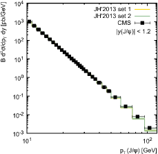
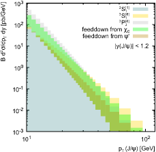
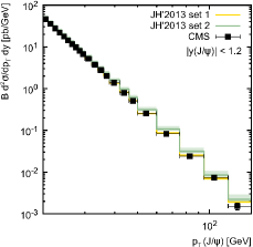
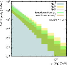
Figure 1: Transverse momentum distribution of prompt $J/\psi$ mesons produced in $pp$ collisions at $\sqrt{s}=7$ TeV (upper plots) and $\sqrt{s}=13$ TeV (lower plots). The shaded bands on the left panels represent the total uncertainties of our calculations (i.e. scale uncertainties and the uncertainties coming from NMEs fit, summed in quadrature), as estimated for JH’2013 set 2 gluon density. The relative contributions from the different production mechanisms are shown on the right panels. The experimental data are from CMS CMS .

To determine the NMEs of $J/\psi$ mesons (as well as their $\eta_{c}$ counterparts) we performed a combined fit of $J/\psi$ and $\eta_{c}$ transverse momentum distributions using the latest CMS CMS , ATLAS ATLAS and LHCb data LHCb collected at 7, 8 and 13 TeV. Here, the factorization principle seems to be on solid theoretical grounds because of not too low $p_{T}$ values for both $J/\psi$ and $\eta_{c}$ mesons. We do not impose any kinematic restrictions but the experimental acceptance. The fitting procedure was separately done in each of the rapidity subdivisions under the requirement that the NMEs be strictly positive, and then the mean-square average of the fitted values was taken. Note that we used the results of a global fit for the entire charmonium family (including, in particular, $\chi_{cJ}$ and $\psi^{\prime}$ states) global to properly calculate the feed-down contributions from $h_{c}$, $\chi_{cJ}$, and $\psi^{\prime}$ decays.

For some (yet unrecognized) reasons, our ${}^{1}P_{1}^{[1]}$ production amplitude (needed to calculate the feed-down $h_{c}\to\eta_{c}\,X$) disagrees with the one found in the literature. Our calculation is off-shell, but has continuous on-shell limit that can be promptly compared with Meijer ; Troost . The contribution is anyway small and unimportant numerically; but the discrepancy is still of interest from the academic point of view. For the lack of details presented in Meijer ; Troost , we cannot repeat their calculation. The details of our calculation are explained in the Appendix.

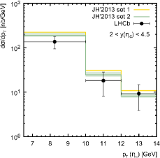
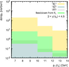
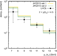
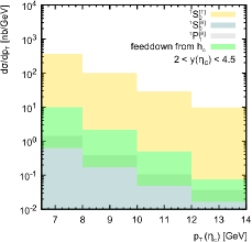
Figure 2: Transverse momentum distribution of prompt $\eta_{c}$ mesons produced in $pp$ collisions at $\sqrt{s}=7$ TeV (upper plots) and $\sqrt{s}=8$ TeV (lower plots). Shaded bands on the left panels represent the total uncertainties of our calculations (i.e. scale uncertainties and the uncertainties coming from NMEs fit, summed in quadrature), as estimated for JH’2013 set 2 gluon density. The relative contributions from the different production mechanisms are shown on the right panels. The experimental data are from LHCb LHCb .

The numerical values of our NMEs for $J/\psi$ and $h_{c}$ mesons are written out in Tables I and II. For comparison, we also present here several sets of NMEs BK ; GW ; chic1 ; chic2 , obtained in the NLO NRQCD by other authors. The NMEs shown for $h_{c}$ mesons are translated from $\chi_{c}$ NMEs using HQSS formulas. The fits differ from one another by somehow differently selected data sets. The corresponding values of NMEs for $\eta_{c}$ meson are collected in Table III. They can be easily obtained from Table I using the HQSS relations (4).

A comparison of our predictions with the experimental results is displayed in Figs. 1 and 2. The theoretical uncertainty bands include both scale uncertainties and the uncertainties coming from the NMEs fitting procedure. First of them were obtained by varying the $\mu_{R}$ scale around its default value by a factor of $2$. This was accompanied with using the JH’2013 set 2+ and JH’2013 set 2- in place of the JH’2013 set 2, in accordance with JH2013 . One can see that we have achieved a reasonably good agreement between our calculations and LHCb measurements (with both of the considered TMD gluons), simultaneously for the prompt $\eta_{c}$ and $J/\psi$ production data collected at different energies and in the whole $p_{T}$ range. The presented results can give a significant impact on the understanding of charmonia production within NRQCD.

Table 2: Sets of NME’s for $h_{c}$ production as determined from the different fits

	JH set 1	JH set 2	Zhang et al. chic1	Likhoded et al. chic2
$\left\langle{\cal O}^{h_{c}}\bigl{[}^{1}P_{1}^{[1]}\bigr{]}\right\rangle/\mbox{GeV}^{5}$	$3.1\pm 0.4$	$3.2\pm 0.5$	0.96	4.51
$\left\langle{\cal O}^{h_{c}}\bigl{[}^{1}S_{0}^{[8]}\bigr{]}\right\rangle/\mbox{GeV}^{3}$	$(6.0\pm 3.0)\cdot 10^{-4}$	$(1.5\pm 0.9)\cdot 10^{-3}$	0.00603	0.00132

IV Conclusions

We have considered the production of charmonium states at the LHC and found a consistent simultaneous description for the $J/\psi$ and $\eta_{c}$ data. Our nonperturbative matrix elements strictly obey the heavy quark spin symmetry rules.

The fundamental difference with the traditional NRQCD scheme (which was unable to accommodate the whole data set) is in a different treatement of the nonperturbative color-octet transitions. The latter are interpreted in our approach in terms of multipole radiation theory. Then the $J/\psi$ mesons are produced unpolarized, thus making no need in a diluting ${}^{1}S_{0}^{[8]}$ contribution to $J/\psi$ production and, as a consequence, requiring no ${}^{3}S_{1}^{[8]}$ contribution to $\eta_{c}$ production. In the forthcoming paper global we are going to present a global fit for the entire charmonium family, including $J/\psi$, $\chi_{cJ}$, $\psi(2S)$ and $\eta_{c}$ mesons.

V Appendix. Off-shell production amplitude for ${}^{1}P_{1}^{[1]}$ state

In this section, we consider the gluon-gluon fusion subprocess

$$g(k_{1},\epsilon_{1},a)+g(k_{2},\epsilon_{2},b)\to g(k_{3},\epsilon_{3},c)+c\bar{c}(p,\epsilon^{\alpha}),$$ (5)

where the symbols in the parentheses indicate the momentum, the polarization, and the color of the interacting quanta. The calculation of this subprocess at ${{\cal O}}(\alpha_{s}^{3})$ relates to six Feynman diagrams:

$${{\cal M}}_{1} = \mbox{tr}\!\left\{\not{\!\epsilon}_{1}(\not{\!p_{c}}-\not{\!k}_{1}+m_{c})\not{\!\epsilon}_{2}(-\not{\!p_{\bar{c}}}-\not{\!k}_{3}+m_{c})\not{\!\epsilon}_{3}\;{{\cal P}}_{S}\right\}$$ (6)

$$\times \left[k_{1}^{2}-2(p_{c}k_{1})\right]^{-1}\left[k_{3}^{2}+2(p_{\bar{c}}k_{3})\right]^{-1},$$

$${{\cal M}}_{2} = \mbox{tr}\!\left\{\not{\!\epsilon}_{1}(\not{\!p_{c}}-\not{\!k}_{1}+m_{c})\not{\!\epsilon}_{3}(-\not{\!p_{\bar{c}}}+\not{\!k}_{2}+m_{c})\not{\!\epsilon}_{2}\;{{\cal P}}_{S}\right\}$$ (7)

$$\times \left[k_{1}^{2}-2(p_{c}k_{1})\right]^{-1}\left[k_{2}^{2}-2(p_{\bar{c}}k_{2})\right]^{-1},$$

$${{\cal M}}_{3} = \mbox{tr}\!\left\{\not{\!\epsilon}_{3}(\not{\!p_{c}}+\not{\!k}_{3}+m_{c})\not{\!\epsilon}_{1}(-\not{\!p_{\bar{c}}}+\not{\!k}_{2}+m_{c})\not{\!\epsilon}_{2}\;{{\cal P}}_{S}\right\}$$ (8)

$$\times \left[k_{3}^{2}+2(p_{c}k_{3})\right]^{-1}\left[k_{2}^{2}-2(p_{\bar{c}}k_{2})\right]^{-1},$$

$${{\cal M}}_{4} = \mbox{tr}\!\left\{\not{\!\epsilon}_{2}(\not{\!p_{c}}-\not{\!k}_{2}+m_{c})\not{\!\epsilon}_{1}(-\not{\!p_{\bar{c}}}-\not{\!k}_{3}+m_{c})\not{\!\epsilon}_{3}\;{{\cal P}}_{S}\right\}$$ (9)

$$\times \left[k_{2}^{2}-2(p_{c}k_{2})\right]^{-1}\left[k_{3}^{2}+2(p_{\bar{c}}k_{3})\right]^{-1},$$

$${{\cal M}}_{5} = \mbox{tr}\!\left\{\not{\!\epsilon}_{2}(\not{\!p_{c}}-\not{\!k}_{2}+m_{c})\not{\!\epsilon}_{3}(-\not{\!p_{\bar{c}}}+\not{\!k}_{1}+m_{c})\not{\!\epsilon}_{1}\;{{\cal P}}_{S}\right\}$$ (10)

$$\times \left[k_{2}^{2}-2(p_{c}k_{2})\right]^{-1}\left[k_{1}^{2}-2(p_{\bar{c}}k_{1})\right]^{-1},$$

$${{\cal M}}_{6} = \mbox{tr}\!\left\{\not{\!\epsilon}_{3}(\not{\!p_{c}}+\not{\!k}_{3}+m_{c})\not{\!\epsilon}_{2}(-\not{\!p_{\bar{c}}}+\not{\!k}_{1}+m_{c})\not{\!\epsilon}_{1}\;{{\cal P}}_{S}\right\}$$ (11)

$$\times \left[k_{3}^{2}+2(p_{c}k_{3})\right]^{-1}\left[k_{1}^{2}-2(p_{\bar{c}}k_{1})\right]^{-1},$$

$${{\cal M}} = {{\cal M}}_{1}+{{\cal M}}_{2}+{{\cal M}}_{3}+{{\cal M}}_{4}+{{\cal M}}_{5}+{{\cal M}}_{6},$$ (12)

with the property ${{\cal M}}_{1}={{\cal M}}_{6}$, ${{\cal M}}_{2}={{\cal M}}_{5}$, ${{\cal M}}_{3}={{\cal M}}_{4}$. The color factor is universal and is equal to $d^{abc}/4\sqrt{3}$. This set of diagrams is complete; no other diagrams can contribute at the order ${{\cal O}}(\alpha_{s}^{3})$ to the production of a meson with the given quantum numbers $J^{PC}=1^{+-}$.

The amplitudes ${{\cal M}}_{i}$ contain spin projection operators which discriminate the spin-singlet and spin-triplet $c\bar{c}$ states:

$${{\cal P}}_{S{=}0} = (\not{\!p_{\bar{c}}}-m_{c})\gamma_{5}(\not{\!p_{c}}+m_{c})\cdot(2m_{c})^{-3/2},$$ (13)

$${{\cal P}}_{S{=}1} = (\not{\!p_{\bar{c}}}-m_{c})\not{\!\epsilon}_{\psi}(\not{\!p_{c}}+m_{c})\cdot(2m_{c})^{-3/2},$$ (14)

where $m_{c}$ is the charmed quark mass. These projectors are orthogonal to each other, as they should be: $tr\{{{\cal P}}_{0}\overline{{{\cal P}}_{1}}\}=0$. For the ${}^{1}P_{1}^{[1]}$ state we evidently have to use the projector ${{\cal P}}_{0}$.

The orbital angular momentum $L$ is associated with the relative momentum $q$ of the quarks in a bound state. The relative momentum $q$ is defined as

$$p_{c}=\frac{1}{2}p+q,\quad p_{\bar{c}}=\frac{1}{2}p-q.$$ (15)

According to a general formalism developed in Guber ; Krase , the terms showing no dependence on $q$ are identified with the contributions to the $L=0$ state; the terms linear in $q^{\alpha}$ are related to the $L=1$ state with the proper polarization vector $\epsilon^{\alpha}$ (see below); the quadratic terms $q^{\alpha}q^{\beta}$ refer to the $L=2$ state with the polarization tensor $\epsilon^{\alpha\beta}$; and so on. The decomposition of ${{\cal M}}$ in powers of $q$ is carried out by expanding the subprocess amplitude as

$${{\cal M}}(q)={{\cal M}}|_{q{=}0}+q^{\alpha}(\partial{{\cal M}}/\partial q^{\alpha})|_{q{=}0}+...,$$ (16)

where $q$ is assumed to be a small quantity. The amplitude ${{\cal M}}(q)$ has to be multiplied by the bound state wave finction $\Psi(q)$ and integrated over $q$. A term-by-term integration of Eq.(16) is performed using the relations

$$\int\frac{d^{3}q}{(2\pi)^{3}}\Psi(q) = \frac{1}{\sqrt{4\pi}}{{\cal R}}(x{=}0),$$ (17)

$$\int\frac{d^{3}q}{(2\pi)^{3}}q^{\alpha}\Psi(q) = -i\epsilon^{\alpha}\frac{\sqrt{3}}{\sqrt{4\pi}}{{\cal R}}^{\prime}(x{=}0),$$ (18)

etc., where ${{\cal R}}(x)$ is the radial wave function in the coordinate representation (the Fourier transform of $\Psi(q)$). This formula completes our derivation of the production matrix element. The resulting expression has been explicitly tested for gauge invariance by substituting the gluon momentum $k_{i}$ for the polarization vector $\epsilon_{i}$. We have observed gauge invariance even with off-shell initial gluons.

Table 3: Sets of NME’s for $\eta_{c}$ production as determined from the different fits

	JH set 1	JH set 2	Kniehl et al. BK	Gong et al. GW
$\left\langle{\cal O}^{\eta_{c}}\bigl{[}^{1}S_{0}^{[1]}\bigr{]}\right\rangle/\mbox{GeV}^{3}$	0.39	0.39	0.44	0.39
$\left\langle{\cal O}^{\eta_{c}}\bigl{[}^{3}S_{1}^{[8]}\bigr{]}\right\rangle/\mbox{GeV}^{3}$	0.0	0.0	0.304	0.097
$\left\langle{\cal O}^{\eta_{c}}\bigl{[}^{1}S_{0}^{[8]}\bigr{]}\right\rangle/\mbox{GeV}^{3}$	$(1.4\pm 0.3)\cdot 10^{-4}$	$(5.3\pm 0.7)\cdot 10^{-4}$	0.00056	-0.0015
$\left\langle{\cal O}^{\eta_{c}}\bigl{[}^{1}P_{1}^{[8]}\bigr{]}\right\rangle/\mbox{GeV}^{5}$	$0.069\pm 0.006$	$0.072\pm 0.006$	-0.02724	-0.0642