COCO-GAN: Generation by Parts via Conditional Coordinating

(Appendix) COCO-GAN: Generation by Parts via Conditional Coordinating

Abstract

Humans can only interact with part of the surrounding environment due to biological restrictions. Therefore, we learn to reason the spatial relationships across a series of observations to piece together the surrounding environment. Inspired by such behavior and the fact that machines also have computational constraints, we propose COnditional COordinate GAN (COCO-GAN) of which the generator generates images by parts based on their spatial coordinates as the condition. On the other hand, the discriminator learns to justify realism across multiple assembled patches by global coherence, local appearance, and edge-crossing continuity. Despite the full images are never generated during training, we show that COCO-GAN can produce state-of-the-art-quality full images during inference. We further demonstrate a variety of novel applications enabled by teaching the network to be aware of coordinates. First, we perform extrapolation to the learned coordinate manifold and generate off-the-boundary patches. Combining with the originally generated full image, COCO-GAN can produce images that are larger than training samples, which we called “beyond-boundary generation”. We then showcase panorama generation within a cylindrical coordinate system that inherently preserves horizontally cyclic topology. On the computation side, COCO-GAN has a built-in divide-and-conquer paradigm that reduces memory requisition during training and inference, provides high-parallelism, and can generate parts of images on-demand.

Chieh Hubert Lin National Tsing Hua University hubert052702@gmail.com	Chia-Che Chang National Tsing Hua University chang810249@gmail.com	Yu-Sheng Chen National Taiwan University nothinglo@ cmlab.csie.ntu.edu.tw
Da-Cheng Juan Google AI dacheng@google.com	Wei Wei Google AI wewei@google.com	Hwann-Tzong Chen National Tsing Hua University htchen@cs.nthu.edu.tw

1 Introduction

The human perception has only partial access to the surrounding environment due to biological restrictions (such as the limited acuity area of the fovea), and therefore humans infer the whole environment by “assembling” few local views obtained from their eyesight. This recognition can be done partially because humans are able to associate the spatial coordination of these local views with the environment (where they are situated in), then correctly assemble these local views, and recognize the whole environment. Currently, most of the computational vision models assume to have access to full images as inputs for down-streaming tasks, which sometimes may become a computational bottleneck of modern vision models when dealing with large field-of-view images. This limitation piques our interest and raises an intriguing question: “is it possible to train generative models to be aware of coordinate system for generating local views (i.e. parts of the image) that can be assembled into a globally coherent image?”

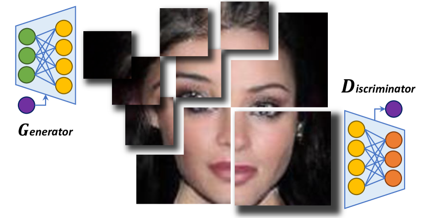
Figure 1: COCO-GAN generates and discriminates only parts of the full image via conditional coordinating. Despite the full images are never generated during training, the generator can still produce full images that are visually indistinguishable to standard GAN samples during inference.

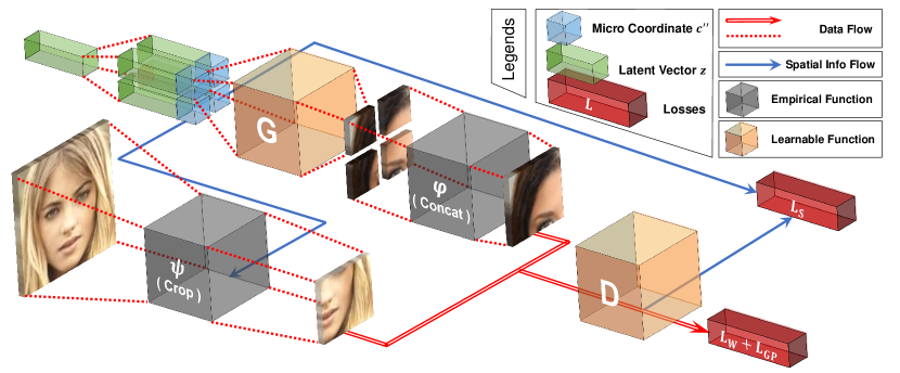
Figure 2: An overview of COCO-GAN training. The latent vectors are duplicated multiple times, concatenated with micro coordinates, and feed to the generator to generate micro patches. Then we concatenate multiple micro patches to form a larger macro patch. The discriminator learns to discriminate between real and fake macro patches and an auxiliary task predicting the coordinate of the macro patch. Note that the full images are only generated in the testing phase (Appendix 12).

Conventional GANs (Goodfellow et al., 2014) target at learning a generator that models a mapping from a prior latent distribution (normally a unit Gaussian) to the real data distribution. To achieve generating high-quality images by parts, we introduce coordinate systems within an image and divide image generation into separated parallel sub-procedures. Our framework, named COnditional COordinate GAN (COCO-GAN), aims at learning a coordinate manifold that is orthogonal to the latent distribution manifold. After a latent vector is sampled, the generator conditions on each spatial coordinate and generate patches at each corresponding spatial position. On the other hand, the discriminator learns to judge whether adjacent patches are structurally sound, visually homogeneous, and continuous across the edges between multiple patches. Figure 1 depicts the high-level idea.

We perform a series of experiments that set the generator to generate patches under different configurations. The results show that COCO-GAN can achieve state-of-the-art generation quality in multiple setups with “Fréchet Inception Distance” (FID) (Heusel et al., 2017) score measurement. Furthermore, to our surprise, even if the generated patch sizes are set to as small as $4\times 4$ pixels, the full images that are composed by 1024 separately generated patches can still consistently form complete and plausible human faces. To further demonstrate the generator indeed learns the coordinate manifold, we perform an extrapolation experiment on the coordinate condition. Interestingly, the generator is able to generate novel contents that are never explicitly presented in the real data. We show that COCO-GAN can produce $384\times 384$ images that are larger than the $256\times 256$ real training samples. We call such a procedure “beyond-boundary generation”; all the samples created through this procedure are guaranteed to be novel samples, which is a powerful example of artificial creativity.

We then investigate another series of novel applications and merits brought about by teaching the network to be aware of the coordinates. The first is panorama generation. To preserve the native horizontally-cyclic topology of panoramic images, we apply cylindrical coordinate to COCO-GAN training process and show that the generated samples are indeed horizontally cyclic. Next, we demonstrate that the “image generation by parts” schema is highly parallelable and saves a significant amount of memory for both training and inference. Furthermore, as the generation procedures of patches are disjoint, COCO-GAN inherently supports generation on-demand, which particularly fits applications for computation-restricted environments, such as mobile and virtual reality. Last but not the least, we show that by adding an extra prediction branch that reconstructs latent vectors, COCO-GAN can generate an entire image with respect to a patch of real image as guidance, which we call “patch-guided generation”.

COCO-GAN unveils the potential of generating high-quality images with conditional coordinating. This property enables a wide range of new applications, and can further be used by other tasks with encoding-decoding schema. With the “generation by parts” property, COCO-GAN is highly parallelable and intrinsically inherits the classic divide-and-conquer design paradigm, which facilitates future research toward large field-of-view data generation.

2 COCO-GAN

Overview.

COCO-GAN consists of two networks (a generator $G$ and a discriminator $D$), two coordinate systems (a finer-grained micro coordinate system for $G$ and a coarser-grained macro coordinate system for $D$), and images of three sizes: full images (real: $x$, generated: $s$), macro patches (real: $x^{\prime}$, generated: $s^{\prime}$) and micro patches (generated: $s^{\prime\prime}$).

The generator of COCO-GAN is a conditional model that generates micro patches with $s^{\prime\prime}=G(z,c^{\prime\prime})$, where $z$ is a latent vector and $c^{\prime\prime}$ is a micro coordinate condition designating the spatial location of $s^{\prime\prime}$ to be generated. The final goal of $G$ is to generate realistic and seamless full images by assembling a set of $s^{\prime\prime}$ altogether with a merging function $\varphi$. In practice, we find that setting $\varphi$ as a concatenation function without overlapping is sufficient for COCO-GAN to synthesize high-quality images. Note that the size of the micro patches and $\varphi$ also imply a cropping transformation $\psi$, cropping out a macro patch $x^{\prime}$ from a real image $x$, which is used to sample real macro patches for training $D$.

In the above setting, the seams between consecutive patches become the major obstacle of full image realism. To mitigate this issue, we train the discriminator with larger macro patches that are assembled with multiple micro patches. Such a design aims to introduce the continuity and coherence of multiple consecutive or nearby micro patches into the consideration of adversarial loss. In order to fool the discriminator, the generator has to close the gap at the boundaries between the generated patches.

COCO-GAN is trained with three loss terms: patch Wasserstein loss $L_{W}$, patch gradient penalty loss $L_{GP}$, and spatial consistency loss $L_{S}$. For $L_{W}$ and $L_{GP}$, compared with conventional GANs that use full images $x$ for both $G$ and $D$ training, COCO-GAN only cooperates with macro patches and micro patches. Meanwhile, the spatial consistency loss $L_{S}$ is an ACGAN-like (Odena et al., 2017) loss function. Depending on the design of $\varphi$, we can calculate macro coordinate $c^{\prime}$ for the macro patches $x^{\prime}$. $L_{S}$ aims at minimizing the distance loss between the real macro coordinate $c^{\prime}$ and the discriminator-estimated macro coordinate $\hat{c}^{\prime}$. The loss functions of COCO-GAN are

$$\begin{cases}L_{W}+\lambda L_{GP}+\alpha L_{S},&\text{for the discriminator}\,D,\\ -L_{W}+\alpha L_{S},&\text{for the generator}\,G.\end{cases}$$ (1)

Spatial coordinate system.

We start with designing the two spatial coordinate systems, a micro coordinate system for the generator $G$ and a macro coordinate system for the discriminator $D$. Depending on the design of the aforementioned merging function $\varphi$, each macro coordinate $c^{\prime}_{(i,j)}$ is associated with a matrix of micro coordinates: ${\bm{C}^{\prime\prime}}_{(i,j)}=\big{[}c^{\prime\prime}_{(i:i+N,j:j+M)}\big{]}$, whose complete form is

$$\scriptsize\bm{C}^{\prime\prime}_{(i,j)}=\begin{bmatrix}c^{\prime\prime}_{(i,j)}&c^{\prime\prime}_{(i,j+1)}&\dots&c^{\prime\prime}_{(i,j+M-1)}\\ c^{\prime\prime}_{(i+1,j)}&c^{\prime\prime}_{(i+1,j+1)}&\dots&c^{\prime\prime}_{(i+1,j+M-1)}\\ \vdots&\vdots&\ddots&\vdots\\ c^{\prime\prime}_{(i+N-1,j)}&c^{\prime\prime}_{(i+N-1,j+1)}&\dots&c^{\prime\prime}_{(i+N-1,j+M-1)}\end{bmatrix}.$$

During COCO-GAN training, we uniformly sample all combinations of $\bm{C}^{\prime\prime}_{(i,j)}$. The generator $G$ conditions on each micro coordinate $c^{\prime\prime}_{(i,j)}$, and learns to accordingly produce micro patches $s^{\prime\prime}_{(i,j)}$ by $G(z,c^{\prime\prime}_{(i,j)})$. The matrix of generated micro patches $\bm{S}^{\prime\prime}_{(i,j)}=G(z,\bm{C}^{\prime\prime}_{(i,j)})$ are produced independently while sharing the same latent vector $z$ across the micro coordinate matrix.

The design principle of the $\bm{C}^{\prime\prime}_{(i,j)}$ construction is that, the accordingly generated micro patches $\bm{S}^{\prime\prime}_{(i,j)}$ should be spatially close to each other. Then the micro patches are merged by the merging function $\varphi$ to form a complete macro patch $s^{\prime}_{(i,j)}=\varphi(\bm{S}^{\prime\prime}_{(i,j)})$ as a coarser partial-view of the imagery full-scene. Meanwhile, we assign $s^{\prime}_{(i,j)}$ with a new macro coordinate $c^{\prime}_{(i,j)}$ under the macro coordinate system with respect to $\bm{C}^{\prime\prime}_{(i,j)}$. On the real data side, we directly sample macro coordinates $c^{\prime}_{(i,j)}$, then produce real macro patches $x^{\prime}_{(i,j)}=\psi(x,c^{\prime}_{(i,j)})$ with the cropping function $\psi$. Note that the design choice of the micro coordinates $\bm{C}^{\prime\prime}_{(i,j)}$ is also correlated with the topological characteristic of the micro/macro coordinate systems (for instance, the cylindrical coordinate system for panoramas used in Section 3.4).

In Figure 2, we illustrate one of the most straightforward designs for the above heuristic functions that we have adopted throughout our experiments. The micro patches are always a neighbor of each other and can be directly combined into a square-shaped macro patch using $\varphi$. We observe that setting $\varphi$ to be a concatenation function is sufficient for $G$ to learn smoothly, and eventually to produce seamless and high-quality images.

During the testing phase, depending on the design of the micro coordinate system, we can infer a corresponding spatial coordinate matrix $\bm{C^{\prime\prime}}_{\textbf{{full}}}$. Such a matrix is used to independently produce all the micro patches required for constituting the full image.

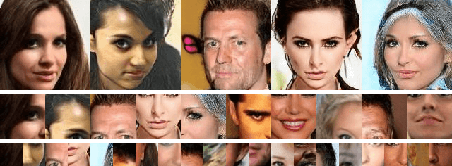
(a) CelebA (N2,M2,S32) (full image: 128$\times$128).

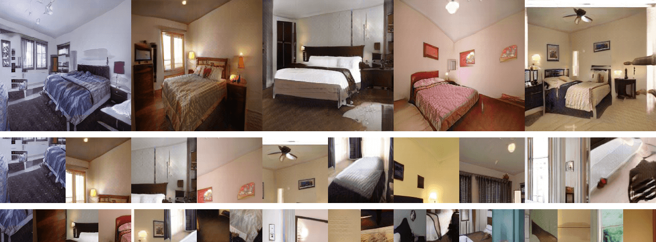
(b) LSUN bedroom (N2,M2,S64) (full image: 256$\times$256).

Figure 3: COCO-GAN generates visually smooth and globally coherent full images without any post-processing. The three rows from top to bottom show: (a) the generated full images, (b) macro patches, and (c) micro patches. For the first five columns, each column uses the same latent vector, e.g., the leftmost full image (first row), the leftmost micro patch (second row), and the leftmost micro patch (third row) share the same latent vector. Note that the columns are not aligned due to different sizes. More results can be found in the Appendix F.

Loss functions.

The patch Wasserstein loss $L_{W}$ is a macro-patch-level Wasserstein distance loss similar to Wasserstein-GAN (Arjovsky et al., 2017) loss. It forces the discriminator to distinguish between the real macro patches $x^{\prime}$ and fake macro patches $s^{\prime}$, and on the other hand, encourages the generator to confuse the discriminator with seemingly realistic micro patches $s^{\prime\prime}$. Its complete form is

$$L_{W}=\displaystyle\mathop{\mathbb{E}}_{x,c^{\prime}}\left[\,D(\psi(x,c^{\prime}))\,\right]-\mathop{\mathbb{E}}_{z,\bm{C}^{\prime\prime}}\left[\,D(\varphi(G(z,\bm{C}^{\prime\prime}))\,\right]\,.$$ (2)

Again, note that $G(z,\bm{C}^{\prime\prime})$ represents that the micro patches are generated through independent processes. We also apply Gradient Penalty (Gulrajani et al., 2017) to the macro patches discrimination:

$$L_{GP}=\displaystyle\mathop{\mathbb{E}}_{\hat{s}^{\prime}}\left[(\|\nabla_{\hat{s}^{\prime}}D(\hat{s}^{\prime})\|_{2}-1)^{2}\right]\,,$$ (3)

where $\hat{s}^{\prime}=\epsilon\,s^{\prime}+(1-\epsilon)\,x^{\prime}$ is calculated between randomly paired $s^{\prime}$ and $x^{\prime}$ with a random number $\epsilon\in\big{[}0,1\big{]}$.

Finally, the spatial consistency loss $L_{S}$ is similar to ACGAN loss (Odena et al., 2017). The discriminator is equipped with an auxiliary prediction head $A$, which aims to estimate the macro coordinate of a given macro patch with $A(x^{\prime})$. A slight difference is that both $c^{\prime\prime}$ and $c^{\prime}$ have relatively more continuous values than the discrete setting of ACGAN. As a result, we apply a distance measurement loss for $L_{S}$, which is an $L_{2}$-loss. It aims to train $G$ to generate corresponding micro patches by $G(z,c^{\prime\prime})$ with respect to the given spatial condition $c^{\prime\prime}$. The spatial consistency loss is

$$L_{S}=\displaystyle\mathop{\mathbb{E}}_{c^{\prime}}\left[\|c^{\prime}-A(x^{\prime})\|_{2}\right]\,.$$ (4)

3 Experiments

3.1 Quality of Generation by Parts

We start with validating COCO-GAN on two common GANs testbeds: CelebA (Liu et al., 2015) and LSUN (Yu et al., 2015) (bedroom). To verify that COCO-GAN can learn to generate the full image without the access to the full image, we first conduct a basic setting for both datasets in which the macro patch edge length (CelebA: $64\times 64$, LSUN: $128\times 128$) is 1/2 of the full image and the micro patch edge length (CelebA: $32\times 32$, LSUN: $64\times 64$) is 1/2 of the macro patch. We denote the above cases as CelebA (N2,M2,S32) and LSUN (N2,M2,S32), where N2 and M2 represent that a macro patch is composed of $2\times 2$ micro patches, and S32 means each of the micro patches is $32\times 32$ pixels. Our results in Figure 3 show that COCO-GAN generates high-quality images in the settings that the micro patch size is 1/16 of the full image.

To further show that COCO-GAN can learn more fine-grained and tiny micro patches under the same macro patch size setting, we sweep through the resolution of micro patch from $32\times 32$, $16\times 16$, $8\times 8$, $4\times 4$, labelled as (N2,M2,S32), (N4,M4,S16), (N8,M8,S8) and (N16,M16,S4), respectively. The results shown in Figure 4 suggest that COCO-GAN can learn coordinate information and generate images by parts even with extremely tiny $4\times 4$ pixels micro patch.

We report Fréchet Inception Distance (FID) (Heusel et al., 2017) in Table 1 comparing with state-of-the-art GANs. Without additional hyper-parameter tuning, the quantitative results show that COCO-GAN is competitive with other state-of-the-art GANs. In Appendix L, we also provide Wasserstein distance and FID score through time as training indicators. The curves suggest that COCO-GAN is stable during training.

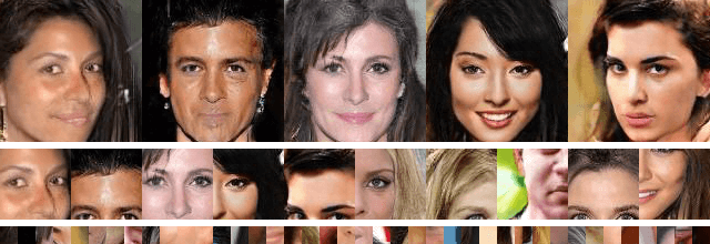
(a) CelebA (N4,M4,S16) (full image: 128$\times$128, FID: 9.99).

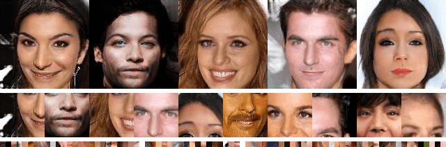
(b) CelebA (N8,M8,S8) (full image: 128$\times$128, FID: 15.99).

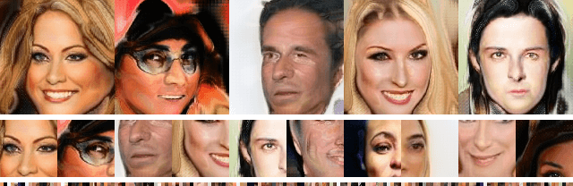
(c) CelebA (N16,M16,S4) (full image: 128$\times$128, FID: 23.90).

Figure 4: Various sizes of micro patches (from $16\times 16$ to $4\times 4$, even smaller than any human face organs) consistently generate visually smooth and globally coherent full images. Each sub-figure consists of three rows, from top to bottom: full images, macro patches, and micro patches. For the first five columns, each column uses the same latent vector (similar with Figure 3). Better to view in high-resolution since the micro patches are very small. More generation results are available in the Appendix F.

Dataset	CelebA 64$\times$64	CelebA 128$\times$128	LSUN Bedroom 64$\times$64	LSUN Bedroom 256$\times$256	CelebA-HQ 1024$\times$1024
DCGAN (Radford et al., 2015) + TTUR (Heusel et al., 2017)	12.5	-	57.5	-
WGAN-GP (Gulrajani et al., 2017) + TTUR (Heusel et al., 2017)	-	-	9.5	-	-
IntroVAE (Huang et al., 2018)	-	-	-	8.84	-
PGGAN (Karras et al., 2017)	-	7.30	-	8.34	7.48
Proj. $D$ (Miyato & Koyama, 2018) (our backbone)	-	19.55	-	-	-
Ours (N2,M2,S32)	4.00	5.74	5.20	5.99∗	9.49∗

Table 1: The FID score suggests that COCO-GAN is competitive with other state-of-the-art generative models. FID scores are measured between 50,000 real and generated samples based on the original implementation provided at https://github.com/bioinf-jku/TTUR. Note that all the FID scores (except proj. $D$) are officially reported numbers. The real samples for evaluation are held-out from training.

3.2 Latent Space Continuity

To demonstrate the space continuity more precisely, we perform the interpolation experiment in two directions: “full-images interpolation” and “coordinates interpolation”.

Full-Images Interpolation.

Intuitively, the inter-full-image interpolation is challenging for COCO-GAN, since all micro patches generated with different spatial coordinates must all change synchronously to make the full-image interpolation smooth. Nonetheless, as shown in Figure 5, we empirically find COCO-GAN can interpolate smoothly and synchronously without producing unnatural artifacts. We randomly sample two latent vectors $z_{1}$ and $z_{2}$. With any given interpolation point $z^{\prime}$ in the slerp-path (White, 2016) between $z_{1}$ and $z_{2}$, the generator uses the full spatial coordinate sequence $\bm{C^{\prime\prime}}_{\textbf{{full}}}$ to generate all corresponding patches. Then we assemble all the generated micro patches together and form a generated full image $s$.

Coordinates Interpolation.

Another dimension of the interpolation experiment is inter-class (e.g. between spatial coordinate condition) interpolation with a fixed latent vector. We linearly-interpolate spatial coordinates between $[-1,1]$ with a fixed latent vector $z$. The results in Figure 6 show that, although we only uniformly sample spatial coordinates within a discrete spatial coordinate set, the spatial coordinates interpolation is still overall continuous.

An interesting observation is about the interpolation at the position between the eyebrows. In Figure 6, COCO-GAN does not know the existence of the glabella between two eyes due to the discrete and sparse spatial coordinates sampling strategy. Instead, it learns to directly deform the shape of the eye to switch from one eye to another. This phenomenon raises an interesting discussion, even though the model learns to produce high-quality face images, it still may learn wrong relationships of objects behind the scene.

Figure 5: The results of full-images interpolation between two latent vectors show that all micro patches are changed synchronously in response to the change of the latent vector. More interpolation results are available in Appendix G.

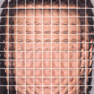
Figure 6: An example of spatial coordinates interpolation showing the spatial continuity of the micro patches. The spatial coordinates are interpolated between range $[-1,1]$ of the micro coordinate with a fixed latent vector. More examples are shown in Appendix I.

3.3 Beyond-Boundary Generation

COCO-GAN enables a new type of image generation that has never been achieved by GANs before: generate full images that are larger than any training sample from scratch. In this context, all the generated images are guaranteed to be novel and original, since these generated images do not even exist in the training distribution. A supportive evidence is that the generated images have higher resolution than any sample in the training data. In comparison, existing GANs mostly have their output shape fixed after its creation and prove the generator can produce novel samples instead of memorizing real data via interpolating between generated samples.

A shared and interesting behavior of learned manifold of GANs is that, in most cases, the generator can still produce plausible samples with latent vectors slightly out of the training distribution, which we called extrapolation. We empirically observe that with a fixed $z$, extrapolation can be done on the coordinate condition beyond the training coordinates distribution. However, as the continuity among patches at these positions is not considered during training, the generated images might show a slight discontinuity at the border. As a solution, we apply a straightforward post-training process (described in Appendix E) for improving the continuity among patches.

In Figure 7, we perform the post-training process on checkpoint of (N4,M4,S64) variant of COCO-GAN that trained on LSUN dataset. Then, we show that COCO-GAN generates high-quality $384\times 384$ images: the original size is 256, with each direction being extended by one micro patch (64 pixels), resulting a size of $384\times 384$. Note that the model is in fact trained on $256\times 256$ images.

Figure 7: “Beyond-Boundary Generation” generates additional contents by extrapolating the learned coordinate manifold. Note that the generated samples are $384\times 384$ pixels, whereas all of the training samples are of a smaller $256\times 256$ resolution. The red box annotates the $256\times 256$ region for regular generation without extrapolation.

3.4 Panorama Generation & Partial Generation

Generating panoramas using GANs is an interesting problem but has never been carefully investigated. Different from normal image generation, panoramas are expected to be cylindrical and cyclic in the horizontal direction. However, normal GANs do not have built-in ability to handle such cyclic characteristic if without special types of padding mechanism support (Cheng et al., 2018). In contrast, COCO-GAN is a coordinate-system-aware learning framework. We can easily adopt a cylindrical coordinate system, and generate panoramas that are having “cyclic topology” in the horizontal direction as shown in Figure 8.

To train COCO-GAN with a panorama dataset under a cylindrical coordinate system, the spatial coordinate sampling strategy needs to be slightly modified. In the horizontal direction, the sampled value within the normalized range $[-1,1]$ is treated as an angular value $\theta$, and then is projected with $\cos(\theta)$ and $\sin(\theta)$ individually to form a unit-circle on a 2D surface. Along with the original sampling strategy on the vertical axis, a cylindrical coordinate system is formed.

We conduct our experiment on Matterport3D (Chang et al., 2017) dataset. We first take the sky-box format of the dataset, which consists of six faces of a 3D cube. We preprocess and project the sky-box to a cylinder using Mercator projection, then resize to $768\times 512$ resolution. Since the Mercator projection creates extreme sparsity near the northern and southern poles, which lacks information, we directly remove the upper and lower $1/4$ areas. Eventually, the size of panorama we use for training is $768\times 256$ pixels.

We also find COCO-GAN has an interesting connection with virtual reality (VR). VR is known to have a tight computational budget due to high frame-rate requirement and high-resolution demand. It is hard to generate full-scene for VR in real time using standard generative models. Some recent VR studies on omnidirectional view rendering and streaming (Corbillon et al., 2017b; Ozcinar et al., 2017; Corbillon et al., 2017a) focus on reducing computational cost or network bandwidth by adapting to the user’s viewport. COCO-GAN, with the generation-by-parts feature, can easily inherit the same strategy and achieve computation on-demand with respect to the user’s viewpoint. Such a strategy can largely reduce unnecessary computational cost outside the region of interest, thus making image generation in VR more applicable.

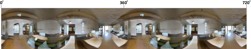
Figure 8: The generated panorama is cyclic in the horizontal direction since COCO-GAN is trained with a cylindrical coordinate system. Here, we paste the same generated panorama twice (from $360^{\circ}$ to $720^{\circ}$) to better illustrate the cyclic property of the generated panorama. More generation results are provided in Appendix H.

3.5 Patch-Guided Image Generation

We further explore an interesting application of COCO-GAN named “Patch-Guided Image Generation”. By training an extra auxiliary network $Q$ within $D$ that predicts the latent vector of each generated macro patch $s^{\prime}$, the discriminator is able to find a latent vector $z_{\textit{est}}=Q(x^{\prime})$ that generates a macro patch similar to a provided real macro patch $x^{\prime}$. Moreover, the estimated latent vector $z_{\textit{est}}$ can be applied to the full-image generation process, and eventually generates an image that is partially similar to the original real macro patch, while globally coherent.

This application shares similar context to some bijection methods (Dumoulin et al., 2017; Donahue et al., 2017; Chang et al., 2018), despite COCO-GAN estimates the latent vector with a single macro patch instead of the full image. In addition, the application is also similar to image restoration (Liu et al., 2018a; Yang et al., 2017; Yeh et al., 2017) or image out-painting (Sabini & Rusak, 2018). However, these related applications heavily rely on the information from the surrounding environment, which is not fully accessible from a single macro patch. In Figure 9, we show that our method is robust to extremely damaged images. More samples and analyses are described in Appendix K.

Macro Patch

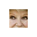
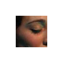
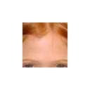
Partial Conv.

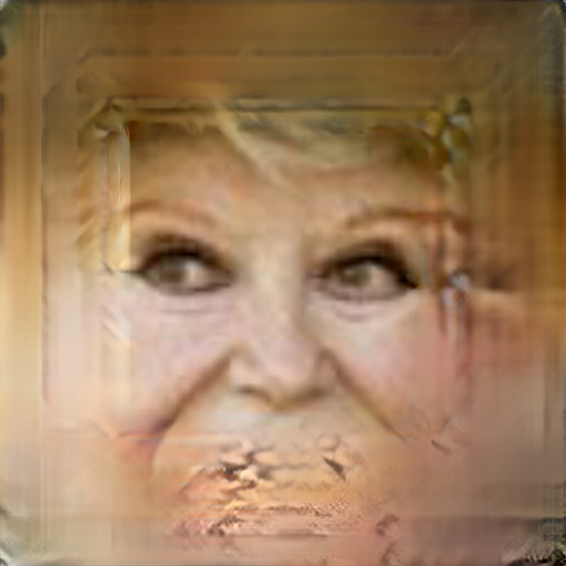
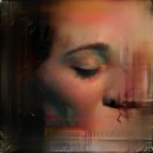
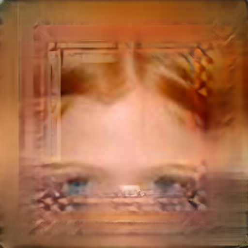
Ours

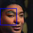
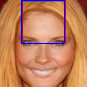
Figure 9: Patch-guided image generation loosely retains the local structures from the original image and make the full image still globally coherent. The quality outperforms the partial convolution (Liu et al., 2018a). The blue boxes visualize the predicted spatial coordinates $A(x^{\prime})$, while the red boxes indicate the ground truth coordinates $c^{\prime}$. Note that the generated images are not expected to be identical to the original real images. More examples are provided in Appendix K.

3.6 Computation-Friendly Generation

Recent studies in high-resolution image generation (Karras et al., 2017; Mescheder et al., 2018; Huang et al., 2018) have gained lots of success; however, a shared conundrum among these existing approaches is the computation being memory hungry. Therefore, these approaches make some compromises to reduce memory usage (Karras et al., 2017; Mescheder et al., 2018). Moreover, this memory bottleneck cannot be easily resolved without specific hardware support, which makes the generation of over $1024\times 1024$ resolution images difficult to achieve. These types of high-resolution images are commonly seen in panoramas, street views, and medical images.

In contrast, COCO-GAN only requires partial views of the full image for both training and inference. Note that the memory consumption for training (and making inference) GANs grows approximately linearly with respect to the image size. Due to using only partial views, COCO-GAN changes the growth in memory consumption to be associated with the size of a macro patch, not the full image. For instance, on the CelebA $128\times 128$ dataset, the (N2,M2,S16) setup of COCO-GAN reduces memory requirement from 17,184 MB (our projection discriminator backbone) to 8,992 MB (i.e., 47.7% reduction), with a batch size 128. However, if the size of a macro patch is too small, COCO-GAN will be misled to learn incorrect spatial relation; in Figure 10, we show an experiment with a macro patch of size $32\times 32$ and a micro patch size of $16\times 16$. Notice the low quality (i.e., duplicated faces). Empirically, the minimum requirement of macro patch size varies for different datasets; for instance, COCO-GAN does not show similar poor quality in panorama generation in Section 3.4, where the macro patch size is 1/48 of the full panorama. Future research on a) how to mitigate such effects (for instance, increase the receptive field of $D$ without harming performance) and b) how to evaluate a proper macro patch size, may further advance the generation-by-parts property particularly in generating large field-of-view data.

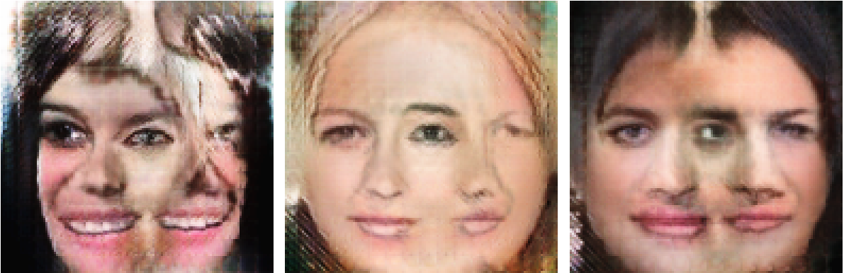
Figure 10: Examples to show that with macro patches smaller than 1/16 of the full image causes COCO-GAN to learn incorrect spatial relation. Note that this value may vary due to the nature (local structure, texture, etc) of each dataset being different.

3.7 Ablation Study

Model	best FID (150 epochs)
COCO-GAN (cont. sampling)	6.13
COCO-GAN + optimal $D$	4.05
COCO-GAN + optimal $G$	6.12
Multiple $G$	7.26
COCO-GAN (N2,M2,S16)	4.87

Table 2: The ablation study shows that COCO-GAN (N2,M2,S16) can converge well with little trade-off in convergence speed on CelebA $64\times 64$ dataset.

In Table 2, the ablation study aims to analyze the trade-offs of each component of COCO-GAN. We perform experiments in CelebA $64\times 64$ with four ablation configurations: “continuous sampling” demonstrates that using continuous uniform sampling strategy for spatial coordinates during training will result in moderate generation quality drop; “optimal $D$” lets the discriminator directly discriminate the full image while the generator still generates micro patches; “optimal $G$” lets the generator directly generate the full image while the discriminator still discriminates macro patches; “multiple $G$” trains an individual generator for each spatial coordinate.

We observe that, surprisingly, despite the convergence speed is different, “optimal discriminator”, COCO-GAN, and “optimal generator” (ordered by convergence speed from fast to slow) can all achieve similar FID scores if with sufficient training time. The difference in convergence speed is expected since “optimal discriminator” provides the generator with more accurate and global adversarial loss. In contrast, the “optimal generator“ has relatively more parameters and layers to optimize, which causes the convergence speed slower than COCO-GAN. Lastly, the “multiple generators” setting cannot converge well. Although it can also concatenate micro patches without obvious seams as COCO-GAN does, the full-image results often cannot agree and are not coherent. More experimental details and generated samples are shown in Appendix J.

3.8 Non-Aligned Dataset

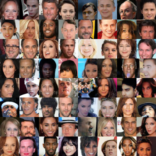
Figure 11: COCO-GAN can learn and synthesis samples with diverse position on the non-aligned Celeba-syn.

It is easy to get confused that the coordinate system would restrain COCO-GAN from learning on less aligned datasets. In fact, this is completely not true. For instance, the bedroom category of LSUN, the location, size and orientation of the bed are very dynamic and non-aligned. On the other hand, the Matterport3D panoramas are completely non-aligned in the horizontal direction.

To further resolve all the potential concerns, we propose CelebA-syn, which applies a random displacement on the raw data (different from data augmentation, this preprocessing directly affects the dataset) to mess up the face alignment. We first trim the raw images to 128$\times$128. The position of the upper-left corner is sampled by $(x,y)=(25+dx,50+dy)$, where $dx\sim\mathcal{U}(-25,25)$ and $dy\sim\mathcal{U}(-25,25)$. Then we resize the trimmed images to 64$\times$64 for training. As shown in Figure 11, COCO-GAN can stably create reasonable samples of high diversity (also notice the high diversity at the eye positions).

4 Related Work

Generative Adversarial Network (GAN) (Goodfellow et al., 2014) and its conditional variant (Mirza & Osindero, 2014) have shown their potential and flexibility to many different tasks. Recent studies on GANs are focusing on generating high-resolution and high-quality synthetic images in different settings. For instance, generating images with $1024\times 1024$ resolution  (Karras et al., 2017; Mescheder et al., 2018), generating images with low-quality synthetic images as condition (Shrivastava et al., 2017), and by applying segmentation maps as conditions (Wang et al., 2017). However, these prior works share similar assumptions: the model must process and generate the full image in a single shot. This assumption consumes an unavoidable and significant amount of memory when the size of the targeting image is relatively large, and therefore makes it difficult to satisfy memory requirements for both training and inference. Searching for a solution to this problem is one of the initial motivations of this work.

COCO-GAN shares some similarities to Pixel-RNN (van den Oord et al., 2016), which is a pixel-level generation framework while COCO-GAN is a patch-level generation framework. Pixel-RNN transforms the image generation task into a sequence generation task and maximizes the log-likelihood directly. In contrast, COCO-GAN aims at decomposing the computation dependencies between micro patches across the spatial dimensions, and then uses the adversarial loss to ensure smoothness between adjacent micro patches.

CoordConv (Liu et al., 2018b) is another similar method but with fundamental differences. CoordConv provides spatial positioning information directly to the convolutional kernels in order to solve the coordinate transform problem and shows multiple improvements in different tasks. In contrast, COCO-GAN uses spatial coordinates as an auxiliary task for the GANs training, which enforces both the generator and the discriminator to learn coordinating and correlations between the generated micro patches. We have also considered incorporating CoordConv into COCO-GAN. However, empirical results show little visual improvement.

5 Conclusion and Discussion

In this paper, we propose COCO-GAN, a novel GAN incorporating the conditional coordination mechanism. COCO-GAN enables “generation by parts” and demonstrates the generation quality being competitive to state-of-the-arts. COCO-GAN also enables several new applications such as “Beyond-Boundary Generation” and “Panorama Generation”, which serve as intriguing directions for future research on leveraging the learned coordinate manifold for (a) tackling with large field-of-view generation and (b) reducing computational requisition.

Particularly, given a random latent vector, Beyond-Boundary Generation generates images larger than any training sample by extrapolating the learned coordinate manifold, which is enabled exclusively by COCO-GAN. Future research on extending this property to other tasks or applications may further take advantage of such an out-of-distribution generation paradigm.

We show that COCO-GAN produces $128\times 128$ images with micro patches as small as $4\times 4$ pixels. The overall FID score slightly degrades due to the small micro patch size. Further studies on the relationship between the patch size and generation stability are left as a straight-line future work.

Although COCO-GAN has achieved a high generation quality comparable to state-of-the-art GANs, for several generated samples we still observe that the local structures may be discontinued or mottled. This suggests further studies on additional refinements or blending approaches that could be applied on COCO-GAN for generating more stable and reliable samples.

6 Acknowledgement

We sincerely thank David Berthelot and Mong-li Shih for the insightful suggestions and advice. We are grateful to the National Center for High-performance Computing for computer time and facilities. Hwann-Tzong Chen was supported in part by MOST grants 107-2634-F-001-002 and 107-2218-E-007-047.

Appendix A COCO-GAN during Testing Phase

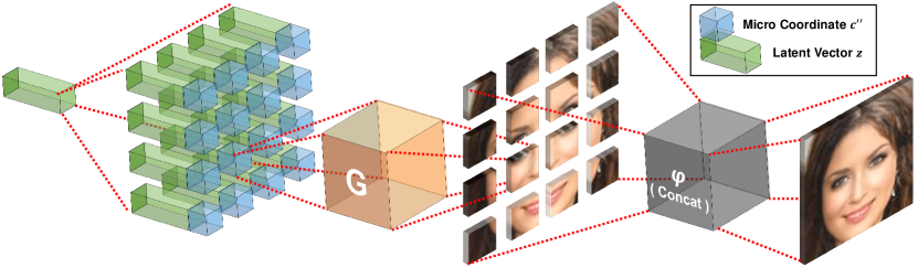
Figure 12: An overview of COCO-GAN during testing phase. The micro patches generated by $G$ are directly combined into a full image as the final output.

Appendix B Symbols

Group	Symbol	Name	Description	Usage
Model	$G$	Generator	Generates micro patches.	$s^{\prime\prime}=G(z,c^{\prime\prime})$
	$D$	Discriminator	Discriminates macro patches.	$D(\varphi(G(z,\bm{C^{\prime\prime}})))$
	$A$	Spatial prediction head	Predicts coordinate of a given macro patch.	$\hat{c}^{\prime}=A(x^{\prime})$
	$Q$	†Content prediction head	Predicts latent vector of a given macro patch.	$z_{est}=Q(s^{\prime})$
Heuristic Function	$\varphi$	Merging function	Merges multiple $s^{\prime\prime}$ to form a $s^{\prime}$ or $s$.	$s^{\prime}=\varphi(G(z,\bm{C^{\prime\prime}}))$
	$\psi$	Cropping function	Crops $x^{\prime}$ from $x$. Corresponding to $\varphi$.	$x^{\prime}=\psi(x,c^{\prime})$
Variable	$z$	Latent vector	Latent variable shared among $s^{\prime\prime}$ generation.	$s^{\prime\prime}=G(z,c^{\prime\prime})$
	$z_{est}$	†Predicted $z$	Predicted $z$ of a given macro patch.	$L_{Q}=\mathop{\mathbb{E}}\left[\,\|z-z_{est}\|_{1}\,\right]$
	$c^{\prime}$	Macro coordinate	Coordinate for macro patches on $D$ side.	$L_{S}=\mathop{\mathbb{E}}\left[\,\|c^{\prime}-\hat{c}^{\prime}\|_{2}\,\right]$
	$c^{\prime\prime}$	Micro coordinate	Coordinate for micro patches on $G$ side.	$s^{\prime\prime}=G(z,c^{\prime\prime})$
	$\hat{c}^{\prime}$	Predicted $c^{\prime}$	Coordinate predicted by $A$ with a given $x^{\prime}$.	$L_{S}=\mathop{\mathbb{E}}\left[\,\|c^{\prime}-\hat{c}^{\prime}\|_{2}\,\right]$
	$\bm{C^{\prime\prime}}$	Matrix of $c^{\prime\prime}$	The matrix of $c^{\prime\prime}$ used to generate $\bm{S^{\prime\prime}}$.	$s^{\prime}=\varphi(G(z,\bm{C^{\prime\prime}}))$
Data	$x$	Real full image	Full resolution data, never directly used.	$x^{\prime}=\psi(x,c^{\prime})$
	$x^{\prime}$	Real macro patch	A macro patch of $x$ which $D$ trains on.	$\text{adv}_{x^{\prime}}=D(\psi(x,c^{\prime}))$
	$s^{\prime}$	Generated macro patch	Composed by $s^{\prime\prime}$ generated with $\bm{C^{\prime\prime}}$.	$\text{adv}_{s^{\prime}}=D(s^{\prime})$
	$s^{\prime\prime}$	Generated micro patch	Smallest data unit generated by $G$.	$s^{\prime\prime}=G(z,c^{\prime\prime})$
	$\bm{S}^{\prime\prime}$	Matrix of $s^{\prime\prime}$	Matrix of $s^{\prime\prime}$ generated by $\bm{C^{\prime\prime}}$.	$\bm{S^{\prime\prime}}=G(z,\bm{C^{\prime\prime}})$
	$\hat{s}^{\prime}$	Interpolated macro patch	Interpolation between random $x^{\prime}$ and $s^{\prime}$.	$\hat{s}^{\prime}=\epsilon\,s^{\prime}+(1-\epsilon)\,x^{\prime}$, which $\epsilon\sim\left[0,1\right]$
Loss	$L_{W}$	WGAN loss	The patch-level WGAN loss.	$L_{W}=\mathop{\mathbb{E}}\left[D(x^{\prime})\right]-\mathop{\mathbb{E}}\left[D(s^{\prime})\right]$
	$L_{GP}$	Gradient penalty loss	The gradient penalty loss to stabilize training.	$L_{GP}=\mathop{\mathbb{E}}\left[(\|\nabla_{\hat{s}^{\prime}}D(\hat{s}^{\prime})\|_{2}-1)^{2}\right]$
	$L_{S}$	Spatial consistency loss	Consistency loss of coordinates.	$L_{S}=\mathop{\mathbb{E}}\left[\|c^{\prime}-A(x^{\prime})\|_{2}\right]$
	$L_{Q}$	†Content consistency loss	Consistency loss of latent vectors.	$L_{Q}=\mathop{\mathbb{E}}\left[\|z-Q(s^{\prime})\|_{1}\right]$
Hyper- parameter	$\alpha$	Weight of $L_{S}$	Controls the strength of $L_{S}$ (we use 100).	$\begin{cases}L_{W}+\lambda L_{GP}+\alpha L_{S},&\text{for}\,D,\\ -L_{W}+\alpha L_{S},&\text{for}\,G.\end{cases}$
	$\lambda$	Weight of $L_{GP}$	Controls the strength of $L_{GP}$ (we use 10).
Testing Only	$s$	Generated full image	Composed by $s^{\prime\prime}$ generated with $\bm{C^{\prime\prime}}_{Full}$.	$s=\varphi(G(z,\bm{C^{\prime\prime}}_{Full}))$
	$\bm{C^{\prime\prime}}_{Full}$	Matrix of $c^{\prime\prime}$ for testing	The matrix of $c^{\prime\prime}$ used during testing.	$s=\varphi(G(z,\bm{C^{\prime\prime}}_{Full}))$

^† Only used in “Patch-Guided Image Generation” application.

Appendix C Experiments Setup and Model Architecture Details

Architecture. Our $G$ and $D$ design uses projection discriminator (Miyato & Koyama, 2018) as the backbone and adding class-projection to the discriminator. All convolutional and feed-forward layers of generator and discriminator are added with the spectral-normalization (Miyato et al., 2018) as suggested in (Zhang et al., 2018). Detailed architecture diagram is illustrated in Figure 13 and Figure 14. Specifically, we directly duplicate/remove the last residual block if we need to enlarge/reduce the size of output patch. However, for (N8,M8,S8) and (N16,M16,S4) settings, since the model becomes too shallow, we keep using (N4,M4,S16) architecture, but without strides in the last one and two layer(s), respectively.

Conditional Batch Normalization (CBN). We follow the projection discriminator that employs CBN (Dumoulin et al., 2016; de Vries et al., 2017) in the generator. The concept of CBN is to normalize, then modulate the features by conditionally produce $\gamma$ and $\beta$ that used in conventional batch normalization, which computes $o_{K}=((i_{K}-\mu_{K})/\sigma_{K})*\gamma+\beta$ for the K-th input feature $i_{K}$, output feature $o_{K}$, feature mean $\mu_{K}$ and feature variance $\sigma_{K}$. However, in the COCO-GAN setup, we provide both spatial coordinate and latent vector as conditional inputs, which both having real values instead of common discrete classes. As a result, we create two MLPs, $\mathrm{MLP}_{\gamma}(z,c)$ and $\mathrm{MLP}_{\beta}(z,c)$, for each CBN layer, that conditionally produces $\gamma$ and $\beta$.

Hyperparameters. For all the experiments, we set the gradient penalty weight $\lambda=10$ and auxiliary loss weight $\alpha=100$. We use Adam (Kingma & Ba, 2014) optimizer with $\beta_{1}=0$ and $\beta_{2}=0.999$ for both the generator and the discriminator. The learning rates are based on the Two Time-scale Update Rule (TTUR) (Heusel et al., 2017), setting $0.0001$ for the generator and $0.0004$ for the discriminator as suggested in (Zhang et al., 2018). We do not specifically balance the generator and the discriminator by manually setting how many iterations to update the generator once as described in the WGAN paper (Arjovsky et al., 2017).

Coordinate Setup. For the micro coordinate matrix $\bm{C}^{\prime\prime}_{(i,j)}$ sampling, although COCO-GAN framework supports real-valued coordinate as input, however, with sampling only the discrete coordinate points that is used in the testing phase will result in better overall visual quality. As a result, all our experiments select to adopt such discrete sampling strategy. We show the quantitative degradation in the ablation study section. To ensure that the latent vectors $z$, macro coordinate conditions $c^{\prime}$, and micro coordinate conditions $c^{\prime\prime}$ share the similar scale, which $z$ and $c^{\prime\prime}$ are concatenated before feeding to $G$. We normalize $c^{\prime}$ and $c^{\prime\prime}$ values into range $[-1,1]$, respectively. For the latent vectors $z$ sampling, we adopts uniform sampling between $[-1,1]$, which is numerically more compatible with the normalized spatial condition space.

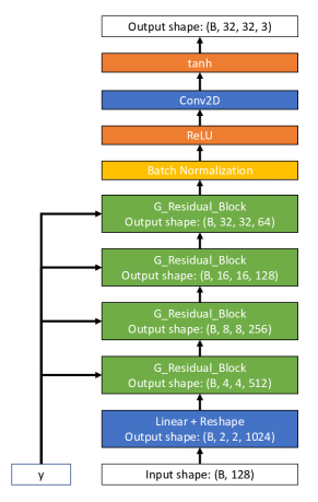
(a) Generator Overall Architecture

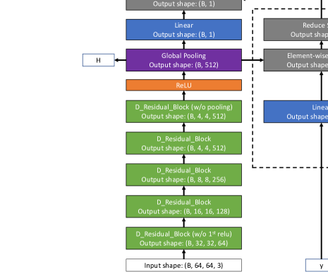
(b) Generator Residual Block

Figure 13: The detailed generator architecture of COCO-GAN for generating micro patches with a size of $32\times 32$ pixels.

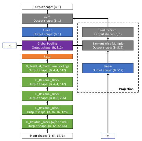
(a) Discriminator Overall Architecture

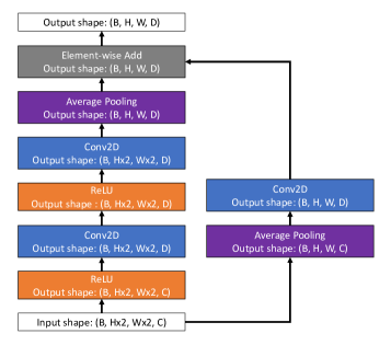
(b) Discriminator Residual Block

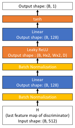
(c) Discriminator Auxiliary Head

Figure 14: The detailed discriminator architecture of COCO-GAN for discriminate macro patches with a size of $64\times 64$ pixels. Both the content vector prediction head ($Q$) and the spatial condition prediction head use the same structure shown in (c).

Appendix D Example of Coordinate Design

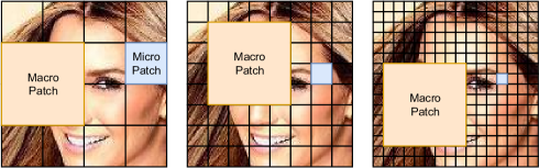
(a) Implementations used in this paper with (Left) P4x4, (Middle) P8x8 and (Right) P16x16.

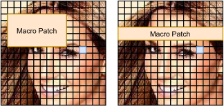
(b) Other possible implementations (not used in this paper).

Figure 15: We showcase some of the coordinate systems: (a) implementations we used in our experiments, and (b) some of the other possible implementations. For instance, 3D cubic data may choose to use each of its face as a macro patch. Also, a recent work (Sun et al., 2019) shows that horizontal tiles are naturally suitable for indoor layout task on panoramas, which points out that using horizontal tiles as macro patch in panorama generation may be an interesting future direction.

Appendix E Beyond-Boundary Generation: More Examples and Details of Post-Training

Figure 16: Without any extra training, original COCO-GAN can already perform slight extrapolations (i.e. the edge of the bed extends out of the normal generation area annotated with the red box), however, expectedly discontinuous on the edges.

We show more examples of “Beyond-Boundary Generation” in Figure 17.

Directly train with coordinates out of the $[-1,1]$ range (restricted by the real full images) is infeasible, since there is no real data at the coordinates outside of the boundary, thus the generator can exploit the discriminator easily. However, interestingly, we find extrapolating the coordinates of a manually trained COCO-GAN can already produce contents that seemingly extended from the edge of the generated full images (e.g., Figure 16).

With such an observation, we select to perform additional post-training on the checkpoint(s) of manually trained COCO-GAN (e.g., (N2,M2,S64) variant of COCO-GAN that trained on LSUN dataset for 1 million steps with resolution $256\times 256$ and a batch size 128). Aside from the original Adam optimizer that trains COCO-GAN with coordinates $\in\left[-1,1\right]$, we create another Adam optimizer with the default learning rate setup (i.e., $0.0004$ for $D$ and $0.0001$ for $G$). The additional optimizer trains COCO-GAN with additional coordinates along with the original coordinates. For instance, in our experiments, we extend an extra micro patch out of the image boundary, as a result, we train the model with $c^{\prime\prime}\in\left[-1.\overline{66},1.\overline{66}\right]$ (the distance between two consecutive micro patches is $2/(4-1)=0.\overline{66}$) and $c^{\prime}\in[-2,2]$ (the distance between two consecutive macro patches is $2/((4-1)-1)=1$). We only use the new optimizer to train COCO-GAN until the discontinuity becomes patches becomes invisible. Note that we do not train the spatial prediction head $A$ with coordinates out of $\left[-1,1\right]$, since our original model has a tanh activation function on the output of $A$, which is impossible to produce predictions out of the range of $\left[-1,1\right]$.

We empirically observe that by only training the first-two layers of the generator (while the whole discriminator at the same time) can largely stabilize the post-training process. Otherwise, the generator will start to produce weird and mottled artifacts. As the local textures are handled by later layers of the generator, we decide to freeze all the later layers and only train the first-two layers, which controls the most high-level representations. We flag the more detailed investigation on the root-cause of such an effect and other possible solutions as interesting future research direction.

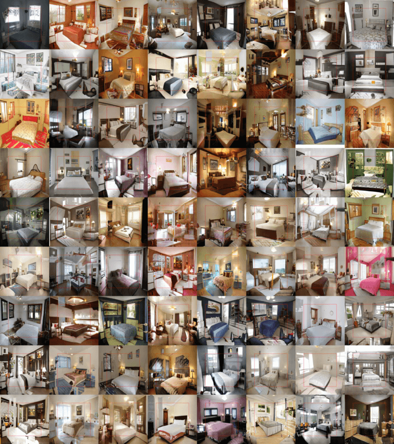
Figure 17: “Beyond-Boundary Generation” generates additional contents by extrapolating the learned coordinate manifold. Note that the generated samples are $384\times 384$ pixels, whereas all of the training samples are of a smaller $256\times 256$ resolution. The red box annotates the $256\times 256$ region for regular generation without extrapolation.

Appendix F More Full Image Generation Examples

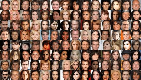
(a) Selected generation samples.

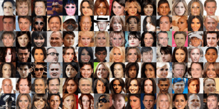
(b) Random generation without calibration.

(c) Generated micro patches.

Figure 18: Full images generated by COCO-GAN on CelebA $128\times 128$ with (N2,M2,S32) setting.

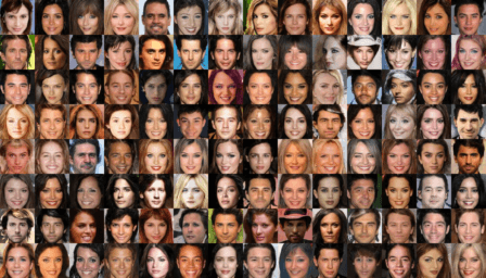
(a) Selected generation samples.

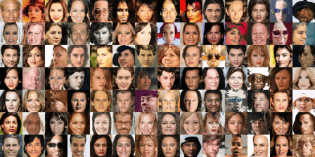
(b) Random generation without calibration.

(c) Generated micro patches.

Figure 19: Full images generated by COCO-GAN on CelebA $128\times 128$ with (N4,M4,S16) setting.

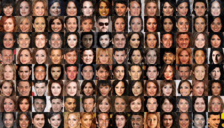
(a) Selected generation samples.

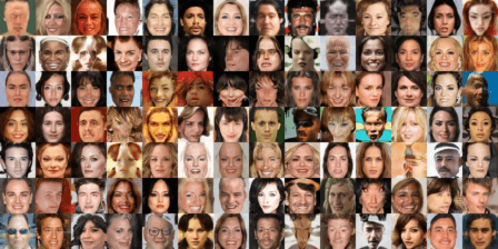
(b) Random generation without calibration.

(c) Generated micro patches.

Figure 20: Full images generated by COCO-GAN on CelebA $128\times 128$ with (N8,M8,S8) setting.

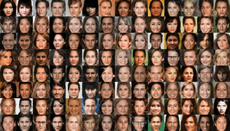
(a) Selected generation samples.

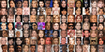
(b) Random generation without calibration.

(c) Generated micro patches.

Figure 21: Full images generated by COCO-GAN on CelebA $128\times 128$ with (N16,M16,S4) setting.

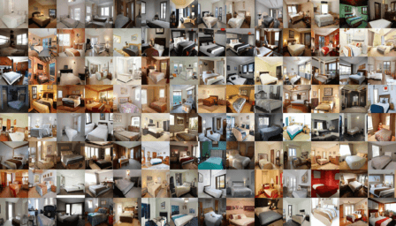
(a) Selected generation samples.

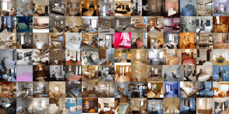
(b) Random generation without calibration.

(c) Generated micro patches.

Figure 22: Full images generated by COCO-GAN on LSUN $256\times 256$ with (N4,M4,S64) setting.

Appendix G More Interpolation Examples

Micro Patches Interpolation

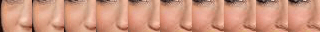
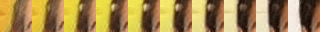
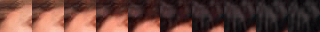
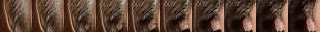
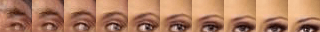
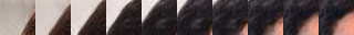
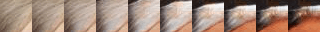
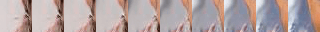
Full-Images Interpolation

(a) CelebA ($128\times 128$).

Micro Patches Interpolation

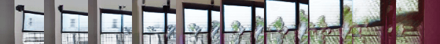
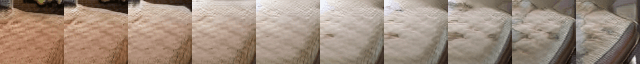
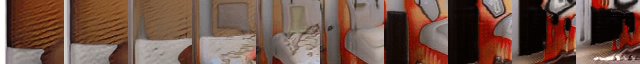
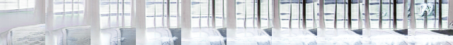
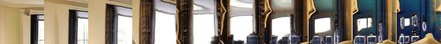
Full-Images Interpolation

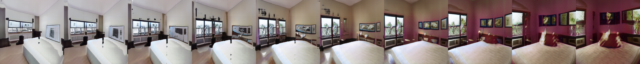
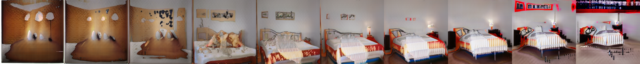
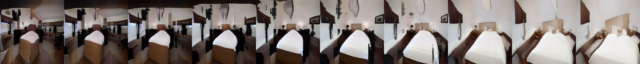
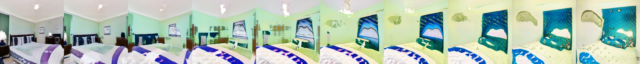
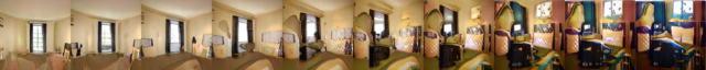
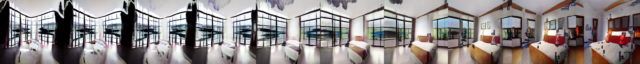
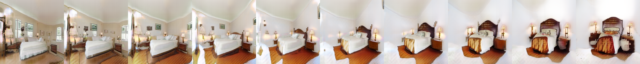
(b) LSUN (bedroom category) ($256\times 256$).

Figure 23: More interpolation examples. Given two latent vectors, COCO-GAN generates the micro patches and full images that correspond to the interpolated latent vectors.

Appendix H More Panorama Generation Samples

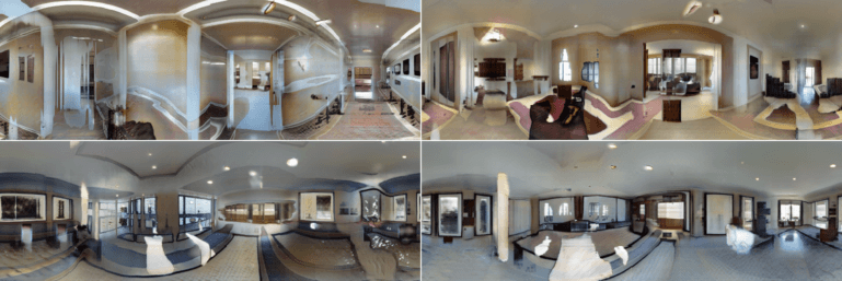
Figure 24: More examples of generated panoramas. All samples possess the cyclic property along the horizontal direction. Each sample is generated with a resolution of $768\times 256$ pixels, and micro patch size $64\times 64$ pixels.

Appendix I Spatial Coordinates Interpolation

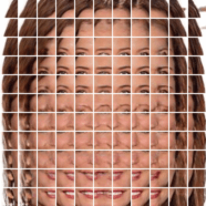
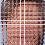
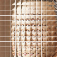
Figure 25: Spatial interpolation shows the spatial continuity of the micro patches. The spatial conditions are interpolated between range $[-1,1]$ of the micro coordinate with a fixed latent vector.

Appendix J Ablation Study

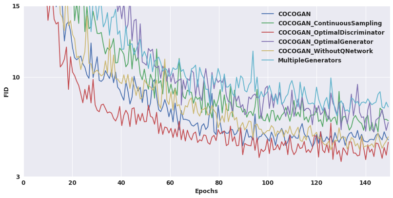
Figure 26: FID score curves of different variants of COCO-GAN in CelebA $64\times 64$ setting. Combined with Figure 27, the results do not show significant differences in quality between COCO-GAN variants. Therefore, COCO-GAN does not pay significant trade-off for the conditional coordinate property.

(a) COCO-GAN (ours).

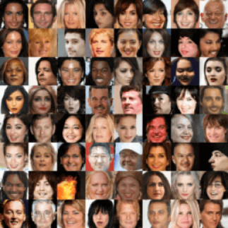
(b) COCO-GAN (cont sampling).

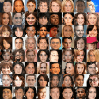
(c) COCO-GAN (optimal $D$).

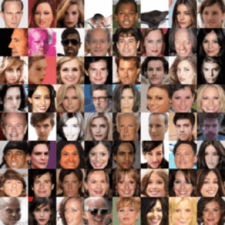
(d) COCO-GAN (optimal $G$).

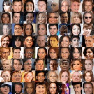
(e) Multiple generators.

Figure 27: Some samples generated by different variants of COCO-GAN. Note that each set of samples is extracted at the epoch when each model variant reaches its lowest FID score. We also provide more samples for each of the variants at different epochs via following : https://goo.gl/Wnrppf.

Appendix K Patch-Guided Image Generation

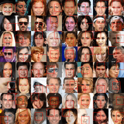
(a) (CelebA 128$\times$128) Real full images.

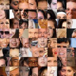
(b) (CelebA 128$\times$128) Real macro patches.

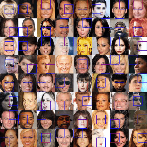
(c) (CelebA 128$\times$128) Patch-guided full image generation.

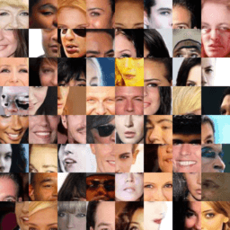
(d) (CelebA 128$\times$128) Patch-guided macro patch generation.

Figure 28: Patch-guided image generation can loosely retain some local structure or global characteristic of the original image. (b) shows the patch-guided generated images based on $z_{\textit{est}}$ estimated from (a). The blue boxes visualize the predicted spatial coordinates $A(x^{\prime})$, while the red boxes indicates the ground truth coordinates $c^{\prime}$. Since the information loss of cropping the macro patches from real images is critical, we do not expect (b) to be identical to the original real image. Instead, the area within blue boxes of (b) should be visually similar to (a), in the meanwhile, (b) should be globally coherent.

Appendix L Training Indicators

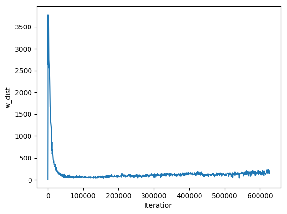
(a) Wasserstein distance

(b) FID

Figure 29: Both Wasserstein distance and FID through time show that the training of COCO-GAN is stable. Both two figures are logged while training on CelebA with $128\times 128$ resolution.

References

- Arjovsky et al. (2017) Arjovsky, M., Chintala, S., and Bottou, L. Wasserstein generative adversarial networks. In Proceedings of the 34th International Conference on Machine Learning, ICML 2017, Sydney, NSW, Australia, 6-11 August 2017, pp. 214–223, 2017.
- Chang et al. (2017) Chang, A. X., Dai, A., Funkhouser, T. A., Halber, M., Nießner, M., Savva, M., Song, S., Zeng, A., and Zhang, Y. Matterport3d: Learning from RGB-D data in indoor environments. In 2017 International Conference on 3D Vision, 3DV 2017, Qingdao, China, October 10-12, 2017, pp. 667–676, 2017.
- Chang et al. (2018) Chang, C.-C., Hubert Lin, C., Lee, C.-R., Juan, D.-C., Wei, W., and Chen, H.-T. Escaping from collapsing modes in a constrained space. In The European Conference on Computer Vision (ECCV), September 2018.
- Cheng et al. (2018) Cheng, H.-T., Chao, C.-H., Dong, J.-D., Wen, H.-K., Liu, T.-L., and Sun, M. Cube padding for weakly-supervised saliency prediction in 360° videos. In The IEEE Conference on Computer Vision and Pattern Recognition (CVPR), June 2018.
- Corbillon et al. (2017a) Corbillon, X., Devlic, A., Simon, G., and Chakareski, J. Optimal set of 360-degree videos for viewport-adaptive streaming. In Proceedings of the 2017 ACM on Multimedia Conference, MM 2017, Mountain View, CA, USA, October 23-27, 2017, pp. 943–951, 2017a.
- Corbillon et al. (2017b) Corbillon, X., Simon, G., Devlic, A., and Chakareski, J. Viewport-adaptive navigable 360-degree video delivery. In IEEE International Conference on Communications, ICC 2017, Paris, France, May 21-25, 2017, pp. 1–7, 2017b.
- de Vries et al. (2017) de Vries, H., Strub, F., Mary, J., Larochelle, H., Pietquin, O., and Courville, A. C. Modulating early visual processing by language. In Advances in Neural Information Processing Systems 30: Annual Conference on Neural Information Processing Systems 2017, 4-9 December 2017, Long Beach, CA, USA, pp. 6597–6607, 2017.
- Donahue et al. (2017) Donahue, J., Krähenbühl, P., and Darrell, T. Adversarial feature learning. In International Conference on Learning Representations, 2017. URL https://openreview.net/forum?id=BJtNZAFgg.
- Dumoulin et al. (2016) Dumoulin, V., Shlens, J., and Kudlur, M. A learned representation for artistic style. CoRR, abs/1610.07629, 2016.
- Dumoulin et al. (2017) Dumoulin, V., Belghazi, I., Poole, B., Lamb, A., Arjovsky, M., Mastropietro, O., and Courville, A. Adversarially learned inference. In International Conference on Learning Representations, 2017. URL https://openreview.net/forum?id=B1ElR4cgg.
- Goodfellow et al. (2014) Goodfellow, I. J., Pouget-Abadie, J., Mirza, M., Xu, B., Warde-Farley, D., Ozair, S., Courville, A. C., and Bengio, Y. Generative adversarial nets. In Advances in Neural Information Processing Systems 27: Annual Conference on Neural Information Processing Systems 2014, December 8-13 2014, Montreal, Quebec, Canada, pp. 2672–2680, 2014.
- Gulrajani et al. (2017) Gulrajani, I., Ahmed, F., Arjovsky, M., Dumoulin, V., and Courville, A. C. Improved training of wasserstein gans. In Advances in Neural Information Processing Systems 30: Annual Conference on Neural Information Processing Systems 2017, 4-9 December 2017, Long Beach, CA, USA, pp. 5769–5779, 2017.
- Heusel et al. (2017) Heusel, M., Ramsauer, H., Unterthiner, T., Nessler, B., and Hochreiter, S. Gans trained by a two time-scale update rule converge to a local nash equilibrium. In Advances in Neural Information Processing Systems 30: Annual Conference on Neural Information Processing Systems 2017, 4-9 December 2017, Long Beach, CA, USA, pp. 6629–6640, 2017.
- Huang et al. (2018) Huang, H., Li, Z., He, R., Sun, Z., and Tan, T. Introvae: Introspective variational autoencoders for photographic image synthesis. In Advances in Neural Information Processing Systems 31: Annual Conference on Neural Information Processing Systems 2018, NeurIPS 2018, 3-8 December 2018, Montréal, Canada., 2018.
- Karras et al. (2017) Karras, T., Aila, T., Laine, S., and Lehtinen, J. Progressive growing of gans for improved quality, stability, and variation. CoRR, abs/1710.10196, 2017.
- Kingma & Ba (2014) Kingma, D. P. and Ba, J. Adam: A method for stochastic optimization. CoRR, abs/1412.6980, 2014.
- Liu et al. (2018a) Liu, G., Reda, F. A., Shih, K. J., Wang, T., Tao, A., and Catanzaro, B. Image inpainting for irregular holes using partial convolutions. CoRR, abs/1804.07723, 2018a.
- Liu et al. (2018b) Liu, R., Lehman, J., Molino, P., Such, F. P., Frank, E., Sergeev, A., and Yosinski, J. An intriguing failing of convolutional neural networks and the coordconv solution. In Advances in Neural Information Processing Systems 31: Annual Conference on Neural Information Processing Systems 2018, NeurIPS 2018, 3-8 December 2018, Montréal, Canada., pp. 9628–9639, 2018b.
- Liu et al. (2015) Liu, Z., Luo, P., Wang, X., and Tang, X. Deep learning face attributes in the wild. In Proceedings of International Conference on Computer Vision (ICCV), December 2015.
- Mescheder et al. (2018) Mescheder, L. M., Geiger, A., and Nowozin, S. Which training methods for gans do actually converge? In Proceedings of the 35th International Conference on Machine Learning, ICML 2018, Stockholmsmässan, Stockholm, Sweden, July 10-15, 2018, pp. 3478–3487, 2018.
- Mirza & Osindero (2014) Mirza, M. and Osindero, S. Conditional generative adversarial nets. CoRR, abs/1411.1784, 2014.
- Miyato & Koyama (2018) Miyato, T. and Koyama, M. cgans with projection discriminator. CoRR, abs/1802.05637, 2018.
- Miyato et al. (2018) Miyato, T., Kataoka, T., Koyama, M., and Yoshida, Y. Spectral normalization for generative adversarial networks. CoRR, abs/1802.05957, 2018.
- Odena et al. (2017) Odena, A., Olah, C., and Shlens, J. Conditional image synthesis with auxiliary classifier gans. In Proceedings of the 34th International Conference on Machine Learning, ICML 2017, Sydney, NSW, Australia, 6-11 August 2017, pp. 2642–2651, 2017.
- Ozcinar et al. (2017) Ozcinar, C., Abreu, A. D., and Smolic, A. Viewport-aware adaptive 360∘ video streaming using tiles for virtual reality. In 2017 IEEE International Conference on Image Processing, ICIP 2017, Beijing, China, September 17-20, 2017, pp. 2174–2178, 2017.
- Radford et al. (2015) Radford, A., Metz, L., and Chintala, S. Unsupervised representation learning with deep convolutional generative adversarial networks. CoRR, abs/1511.06434, 2015.
- Sabini & Rusak (2018) Sabini, M. and Rusak, G. Painting outside the box: Image outpainting with gans. arXiv preprint arXiv:1808.08483, 2018.
- Shrivastava et al. (2017) Shrivastava, A., Pfister, T., Tuzel, O., Susskind, J., Wang, W., and Webb, R. Learning from simulated and unsupervised images through adversarial training. In 2017 IEEE Conference on Computer Vision and Pattern Recognition, CVPR 2017, Honolulu, HI, USA, July 21-26, 2017, pp. 2242–2251, 2017.
- Sun et al. (2019) Sun, C., Hsiao, C.-W., Sun, M., and Chen, H.-T. Horizonnet: Learning room layout with 1d representation and pano stretch data augmentation. arXiv preprint arXiv:1901.03861, 2019.
- van den Oord et al. (2016) van den Oord, A., Kalchbrenner, N., and Kavukcuoglu, K. Pixel recurrent neural networks. In Proceedings of the 33nd International Conference on Machine Learning, ICML 2016, New York City, NY, USA, June 19-24, 2016, pp. 1747–1756, 2016.
- Wang et al. (2017) Wang, T., Liu, M., Zhu, J., Tao, A., Kautz, J., and Catanzaro, B. High-resolution image synthesis and semantic manipulation with conditional gans. CoRR, abs/1711.11585, 2017.
- White (2016) White, T. Sampling generative networks: Notes on a few effective techniques. CoRR, abs/1609.04468, 2016.
- Yang et al. (2017) Yang, C., Lu, X., Lin, Z., Shechtman, E., Wang, O., and Li, H. High-resolution image inpainting using multi-scale neural patch synthesis. In 2017 IEEE Conference on Computer Vision and Pattern Recognition, CVPR 2017, Honolulu, HI, USA, July 21-26, 2017, pp. 4076–4084, 2017.
- Yeh et al. (2017) Yeh, R. A., Chen, C., Lim, T., Schwing, A. G., Hasegawa-Johnson, M., and Do, M. N. Semantic image inpainting with deep generative models. In 2017 IEEE Conference on Computer Vision and Pattern Recognition, CVPR 2017, Honolulu, HI, USA, July 21-26, 2017, pp. 6882–6890, 2017.
- Yu et al. (2015) Yu, F., Zhang, Y., Song, S., Seff, A., and Xiao, J. LSUN: construction of a large-scale image dataset using deep learning with humans in the loop. CoRR, abs/1506.03365, 2015.
- Zhang et al. (2018) Zhang, H., Goodfellow, I. J., Metaxas, D. N., and Odena, A. Self-attention generative adversarial networks. CoRR, abs/1805.08318, 2018.