High harmonic generation in crystals using Maximally Localized Wannier functions

Abstract

In this work, the nonlinear optical response, and in particular, the high harmonic generation of semiconductors is addressed by using the Wannier gauge. One of the main problems in the time evolution of the Semiconductor Bloch equations resides in the fact that the dipole couplings between different bands can diverge and have a random phase along the reciprocal space and this leads to numerical instability. To address this problem, we propose the use of the Maximally Localized Wannier functions that provide a framework to map ab-initio calculations to an effective tight-binding Hamiltonian with great accuracy. We show that working in the Wannier gauge, the basis set in which the Bloch functions are constructed directly from the Wannier functions, the dipole couplings become smooth along the reciprocal space thus avoiding the problem of random phases. High harmonic generation spectrum is computed for a 2D monolayer of hBN as a numerical demonstration.

I Introduction

Since the discovery of high harmonic generation (HHG) in solids (Ghimire et al., 2011), several works demonstrate the potential of analyzing the light emitted by bulk electrons in solids when exposed to intense laser fields. Recent results include the observation of dynamical Bloch oscillations (Schubert et al., 2014; Luu et al., 2015), band structure tomography (Vampa et al., 2015; Tancogne-Dejean et al., 2017), resolving electron-hole dynamics (Bauer and Hansen, 2018; McDonald et al., 2015), including dynamics in strongly correlated systems and phase transitions in the Mott insulator (Silva et al., 2018), the Peierls phase transition (Bauer and Hansen, 2018), or the imprint of the Berry phase on high harmonic spectrum (Luu and Wörner, 2018; Liu et al., 2017).

The first theoretical works trying to describe HHG in solids are previous to the experimental realization of the process (Plaja and Roso-Franco, 1992; Golde et al., 2008). But the interest in the theoretical understanding had grown in the last years (Hawkins and Ivanov, 2013; Vampa et al., 2014; Hawkins et al., 2015; Korbman et al., 2013; Wismer et al., 2016; Floss et al., 2018; Osika et al., 2017; Tancogne-Dejean et al., 2017). Several theoretical approaches were used in this context: solution of the time dependent Schrödinger equation (TDSE) (Korbman et al., 2013), time-dependent density functional theory (TDDFT) (Tancogne-Dejean et al., 2017) and semiconductor Bloch equations (SBE) (Kira and Koch, 2012; Golde et al., 2008).

Despite the variety of theoretical approaches used up to now, the calculation of nonlinear optical properties of crystals presents several difficulties. In the dipole approximation, two different gauges for the electromagnetic field are usually used: length gauge (LG) and velocity gauge (VG). In the VG, the advantage with respect to the LG is that the dynamical equations become decoupled in the Brillouin zone but a large number of bands need to be included in the calculation to obtain the converged result (Aversa and Sipe, 1995; Ventura et al., 2017). On the other hand, the LG gives the converged result for low frequencies with a modest number of bands included in the calculation. In the LG, the problem arises in the representation of the position operator, that now involves a derivative in the Brillouin zone (Blount, 1962). Evaluating this derivative is a numerical challenge since the Bloch eigenstates of the crystalline Hamiltonian are defined up to a random phase in the Brillouin zone. In this work, we propose a way to circumvent this problem by using the Maximally Localized Wannier functions (MLWF) that cure this gauge freedom (Marzari and Vanderbilt, 1997; Marzari et al., 2012). The formalism developed in this work can be applied to analytical tight-binding models but also for DFT calculations that can be mapped to a tight-binding Hamiltonian using the MLWF procedure (Mostofi et al., 2014; Marzari and Vanderbilt, 1997; Marzari et al., 2012).

II Theory

In this section, we give a brief overview of the theory of nonlinear optical response in semiconductors. It is worth to point out the reader to the work of Blount (Blount, 1962) and to the work of Ventura et al. (Ventura et al., 2017; Ventura, 2016) where detailed discussion is given on the difficulties that the position operator presents in a crystal. We derive the dynamical equations for the calculation of the bulk current of a semiconductor when in presence of an intense laser pulse. We will work in the length gauge (LG) under the dipole approximation and neglecting electron-electron and electron-phonon interactions.

The novelty of this work relies on the numerical solution of the dynamical equations in a diabatic basis instead of solving them in an adiabatic basis. As it is well know in molecular physics, the study of molecular dynamics is sometimes cumbersome if one chooses to work with an adiabatic basis, especially when one needs to deal with avoided crossings or conical intersections. It is much more appropriate to study molecular dynamics in a diabatic basis, in which non-adiabatic couplings are absent, or as small as possible (Tannor, 2006). Two major problems arise when calculating the non-adiabatic couplings in the adiabatic basis: the gauge freedom for choosing the eigenstates of the Hamiltonian up to a random phase and the divergences of the non-adiabatic couplings in the vicinity of the avoided crossings or conical intersections.

In a complete analogy with molecular physics, this work proposes a diabatic basis in which the numerical solution of SBE can be achieved easily, the Wannier gauge (Marzari et al., 2012). It must be stressed out that when one is referring to the LG versus the VG, we are dealing with the intrinsic gauge freedom to describe the electromagnetic field. On the other hand, when we are referring to the Hamiltonian gauge versus the Wannier gauge, we are dealing with two different basis set in which we can solve our quantum mechanical problem. The Hamiltonian gauge is a choice of a basis set in which we expand our wavefunction (or density matrix) in Bloch eigenstates of the crystalline Hamiltonian. On the other hand, the Wannier gauge is the gauge in which calculations are done using an expansion on Bloch states that are constructed from localized Wannier orbitals. In analogy with molecular physics, the Hamiltonian gauge is what we would think as an adiabatic basis and the Wannier gauge is what we would think as a diabatic basis.

II.1 Single-Particle Theory

Within the dipole approximation and in the LG, the time-dependent Hamiltonian describing the interaction of an electron in a periodic potential with a laser field is

$$\hat{H}\left(t\right) =\hat{H}_{0}+\left|e\right|\boldsymbol{E}\left(t\right).\hat{\boldsymbol{r}}$$ (II.1)

$$\hat{H}_{0} =\frac{\boldsymbol{p}^{2}}{2m_{e}}+U\left(\boldsymbol{r}\right)$$ (II.2)

$$U\left(\boldsymbol{r}\right) =U\left(\boldsymbol{r}+\boldsymbol{R}\right)$$ (II.3)

where $\boldsymbol{E}\left(t\right)$ is the electric field, $\left|e\right|$ is the elementary charge, $m_{e}$ is the electron mass and $\boldsymbol{R}$ is a Bravais lattice vector. Let us consider a set of $M$ localized Wannier orbitals in each cell $w_{m}\left(\boldsymbol{r}-\boldsymbol{R}\right)=\Braket{\boldsymbol{r}}{\boldsymbol{R}m}$. We assume that these Wannier orbitals form an orthonormal basis, i.e. $\Braket{\boldsymbol{R}^{\prime}n}{\boldsymbol{R}m}=\delta_{n,m}\delta_{\boldsymbol{R^{\prime}},\boldsymbol{R}}$. Assuming that our system contains $N_{c}$ unitary cells with periodic boundary conditions, we can define Bloch like functions from these Wannier orbitals

$$\Ket{\psi_{m\boldsymbol{k}}^{\left(W\right)}} =\frac{1}{\sqrt{N_{c}}}\sum_{\boldsymbol{R}}e^{i\boldsymbol{k}.\boldsymbol{R}}\Ket{\boldsymbol{R}m}$$ (II.4)

$$\Braket{\boldsymbol{r}}{\psi_{m\boldsymbol{k}}^{\left(W\right)}} =\frac{1}{\sqrt{N_{c}V_{c}}}e^{i\boldsymbol{k}.\boldsymbol{r}}u_{m\boldsymbol{k}}^{\left(W\right)}\left(\boldsymbol{r}\right)$$ (II.5)

where $V_{c}$ is the volume of a unit cell and $u_{m\boldsymbol{k}}^{\left(W\right)}\left(\boldsymbol{r}\right)$ is the periodic part of the Bloch function.

We are interested in the calculation of nonlinear optical response within the dipole approximation and for a complete description of the light-matter interaction it is only necessary to have the knowledge of

$$\Braket{\boldsymbol{0}n}{\hat{H}_{0}}{\boldsymbol{R}m}$$ (II.6)

$$\Braket{\boldsymbol{0}n}{\hat{\boldsymbol{r}}}{\boldsymbol{R}m}$$ (II.7)

where $\hat{H}_{0}$ is the unperturbed Hamiltonian and $\hat{\boldsymbol{r}}$ is the position operator. These matrix elements can either be calculated from an electronic structure calculation followed by a wannierization procedure (Marzari et al., 2012) or can be set explicitly by analytical tight-binding models. We can define, as in (Wang et al., 2006), the Hamiltonian and Berry connection matrices in the Wannier gauge

$$H_{nm}^{(W)}\left(\boldsymbol{k}\right) \equiv\sum_{\boldsymbol{R}}e^{i\boldsymbol{k}.\boldsymbol{R}}\left\langle\boldsymbol{0}n\left|\hat{H}_{0}\right|\boldsymbol{R}m\right\rangle$$ (II.8)

$$\boldsymbol{A}_{nm}^{(W)}\left(\boldsymbol{k}\right) \equiv\sum_{\boldsymbol{R}}e^{i\boldsymbol{k}.\boldsymbol{R}}\left\langle\boldsymbol{0}n\left|\hat{\boldsymbol{r}}\right|\boldsymbol{R}m\right\rangle.$$ (II.9)

where the sum in $\boldsymbol{R}$ runs over all lattice vectors in our system and the superscript $\left(W\right)$ refers to the Wannier gauge (as in (Wang et al., 2006)). As it will be seen later, these matrices enter in the dynamical equations of our system. Since we are working under the assumption that the Wannier orbitals are localized functions, we expect that the terms, $\left\langle\boldsymbol{0}n\left|\hat{H}_{0}\right|\boldsymbol{R}m\right\rangle$ and $\left\langle\boldsymbol{0}n\left|\hat{\boldsymbol{r}}\right|\boldsymbol{R}m\right\rangle$, in the sum will decay exponentially with $\boldsymbol{R}$ and this fact will lead to smooth matrices, $H^{(W)}\left(\boldsymbol{k}\right)$ and $\boldsymbol{A}^{(W)}\left(\boldsymbol{k}\right)$.

We can write the single particle unperturbed Hamiltonian as

$$\hat{H}_{0} =\sum_{\boldsymbol{k}\in FBZ}\sum_{n,m}H_{nm}^{(W)}\left(\boldsymbol{k}\right)\Ket{\psi_{n\boldsymbol{k}}^{\left(W\right)}}\Bra{\psi_{m\boldsymbol{k}}^{\left(W\right)}}$$ (II.10)

where the sum over $\boldsymbol{k}$ runs over all allowed crystal momentum inside the first Brillouin zone (FBZ). We can work in the basis where $\hat{H}_{0}$ is diagonal and for that we only need to diagonalize the $H_{nm}^{(W)}\left(\boldsymbol{k}\right)$ matrix. We will refer to this basis as the Hamiltonian gauge using the superscript $\left(H\right)$. Whenever none of the superscripts are used it means that the result is valid for both, $\left(W\right)$ and $\left(H\right)$, gauges. Both basis are related to each other by a unitary transformation

$$\ket{\psi_{n\boldsymbol{k}}^{\left(H\right)}}=\sum_{m}U_{mn}\left(\boldsymbol{k}\right)\ket{\psi_{m\boldsymbol{k}}^{\left(W\right)}}$$ (II.11)

where $U\text{$\left(\boldsymbol{k}\right)$}$ is a unitary matrix that diagonalizes $H^{(W)}\left(\boldsymbol{k}\right)$,

$$U^{\dagger}\text{$\left(\boldsymbol{k}\right)$}H^{(W)}\left(\boldsymbol{k}\right)U\text{$\left(\boldsymbol{k}\right)$}=H^{(H)}\left(\boldsymbol{k}\right).$$ (II.12)

The relationship between the $\boldsymbol{A}\left(\boldsymbol{k}\right)$ matrix in both gauges is (Wang et al., 2006)

$$\boldsymbol{A}^{\left(H\right)}\left(\boldsymbol{k}\right)=U^{\dagger}\text{$\left(\boldsymbol{k}\right)$}\boldsymbol{A}^{\left(W\right)}\left(\boldsymbol{k}\right)U\text{$\left(\boldsymbol{k}\right)$}+iU^{\dagger}\text{$\left(\boldsymbol{k}\right)$}\frac{\partial}{\partial\boldsymbol{k}}U\left(\boldsymbol{k}\right).$$ (II.13)

It must be noted that the matrix $U\left(\boldsymbol{k}\right)$ is not unique. This fact lies on the gauge freedom that we have to choose a global phase for the eigenstates, $\Ket{\psi_{n\boldsymbol{k}}^{\left(H\right)}}\rightarrow e^{i\theta_{n}\left(\boldsymbol{k}\right)}\Ket{\psi_{n\boldsymbol{k}}^{\left(H\right)}}$. Since the last term, $iU^{\dagger}\text{$\left(\boldsymbol{k}\right)$}\frac{\partial}{\partial\boldsymbol{k}}U\left(\boldsymbol{k}\right)$, is not invariant under this phase transformation, we have an intrinsic gauge freedom in the calculation of $\boldsymbol{A}^{\left(H\right)}\left(\boldsymbol{k}\right)$. It is precisely this gauge freedom that we try to avoid using the Wannier gauge.

The matrix elements of the position operator in a finite volume system with periodic boundary conditions are ill-defined, but can be computed in the thermodynamic limit. The representation of the position operator in a Bloch basis is (Blount, 1962; Ventura et al., 2017)

$$\hat{\boldsymbol{r}}=i\frac{\partial}{\partial\boldsymbol{k}}+\hat{\boldsymbol{A}}$$ (II.14)

where $\hat{\boldsymbol{A}}$ is the Berry connection that is defined as

$$\boldsymbol{A}_{nm}\left(\boldsymbol{k}\right)=i\int_{V_{C}}d^{D}\boldsymbol{r}\left(u_{n\boldsymbol{k}}\left(\boldsymbol{r}\right)\right)^{*}\frac{\partial}{\partial\boldsymbol{k}}u_{m\boldsymbol{k}}\left(\boldsymbol{r}\right).$$ (II.15)

In the Wannier gauge the Berry connection will be the one defined in Eq. (II.9).

The matrix representation of the current operator in a Bloch basis is defined as

$$\hat{\boldsymbol{J}} =\frac{-\left|e\right|}{i\hbar}\left[\hat{\boldsymbol{r}},\hat{H}\left(t\right)\right]$$ (II.16)

$$\left(\hat{\boldsymbol{J}}\right)_{\boldsymbol{k},nm} =\frac{-\left|e\right|}{\hbar}\left(\frac{\partial}{\partial\boldsymbol{k}}H_{nm}\left(\boldsymbol{k}\right)-i\left[\boldsymbol{A}\left(\boldsymbol{k}\right),H\left(\boldsymbol{k}\right)\right]_{nm}\right).$$ (II.17)

In the Hamiltonian gauge, we can identify the two terms in the expression for the current as the intraband and interband current.

$$\left(\hat{\boldsymbol{J}}_{intra}\right)_{\boldsymbol{k},nm} =\frac{-\left|e\right|}{\hbar}\left(\frac{\partial}{\partial\boldsymbol{k}}H_{nm}^{\left(H\right)}\left(\boldsymbol{k}\right)\right)$$ (II.18)

$$\left(\hat{\boldsymbol{J}}_{inter}\right)_{\boldsymbol{k},nm} =\frac{i\left|e\right|}{\hbar}\left(\left[\boldsymbol{A}^{\left(H\right)}\left(\boldsymbol{k}\right),H^{\left(H\right)}\left(\boldsymbol{k}\right)\right]_{nm}\right).$$ (II.19)

II.2 Many-body theory

Having all the relevant operators (the current and the time-dependent Hamiltonian operator) defined in first quantization, we proceed to define all the relevant operators in a second quantization formalism. The time-dependent many-body Hamiltonian is just

$$\hat{\mathcal{H}}\left(t\right) =\sum_{\boldsymbol{k}\in FBZ}\sum_{n,m}c_{n\boldsymbol{k}}^{\dagger}H_{nm}\left(\boldsymbol{k}\right)c_{m\boldsymbol{k}}$$

$$+\sum_{\boldsymbol{k}\in FBZ}\sum_{n,m}c_{n\boldsymbol{k}}^{\dagger}\left|e\right|\boldsymbol{E}\left(t\right).\left[i\delta_{nm}\frac{\partial}{\partial\boldsymbol{k}}+\boldsymbol{A}_{nm}\left(\boldsymbol{k}\right)\right]c_{m\boldsymbol{k}}$$ (II.20)

where $c_{n\boldsymbol{k}}^{\dagger}$ ($c_{n\boldsymbol{k}}$) is the fermionic creation (annihilation) operator of a Bloch state. The many-body current operator can also be expressed as

$$\hat{\boldsymbol{\mathcal{J}}} =\sum_{\boldsymbol{k}\in FBZ}\sum_{n,m}\left(\hat{\boldsymbol{J}}\right)_{\boldsymbol{k},nm}c_{n\boldsymbol{k}}^{\dagger}c_{m\boldsymbol{k}}$$ (II.21)

$$=\sum_{\boldsymbol{k}\in FBZ}\sum_{n,m}\frac{-\left|e\right|}{\hbar}\left(\frac{\partial}{\partial\boldsymbol{k}}H_{nm}\left(\boldsymbol{k}\right)\right)c_{n\boldsymbol{k}}^{\dagger}c_{m\boldsymbol{k}}$$

$$+\sum_{\boldsymbol{k}\in FBZ}\sum_{n,m}\frac{i\left|e\right|}{\hbar}\left[\boldsymbol{A}\left(\boldsymbol{k}\right),H\left(\boldsymbol{k}\right)\right]_{nm}c_{n\boldsymbol{k}}^{\dagger}c_{m\boldsymbol{k}}$$ (II.22)

The observables that we are interested in is the mean value of the current operator, $\hat{\left\langle\boldsymbol{\mathcal{J}}\right\rangle}$, and for that we only need to know the mean values of $c_{n\boldsymbol{k}}^{\dagger}c_{m\boldsymbol{k}}$. Let us define the reduced density matrix (RDM) as

$$\rho_{nm}\left(\boldsymbol{k},t\right)=\left\langle c_{m\boldsymbol{k}}^{\dagger}c_{n\boldsymbol{k}}\right\rangle.$$ (II.23)

Note that the band indexes are switched. The equations of motion for the RDM have the following form (Ventura et al., 2017)

$$i\hbar\frac{\partial}{\partial t}\rho_{nm}\left(\boldsymbol{k},t\right) =\left\langle\left[c_{m\boldsymbol{k}}^{\dagger}c_{n\boldsymbol{k}},\hat{\mathcal{H}}\left(t\right)\right]\right\rangle$$

$$=\left[H\left(\boldsymbol{k}\right),\rho\left(\boldsymbol{k},t\right)\right]_{nm}$$

$$+i\left|e\right|\boldsymbol{E}\left(t\right).\frac{\partial}{\partial\boldsymbol{k}}\rho_{nm}\left(\boldsymbol{k},t\right)$$

$$+\left|e\right|\boldsymbol{E}\left(t\right).\left[\boldsymbol{A}\left(\boldsymbol{k}\right),\rho\left(\boldsymbol{k},t\right)\right]_{nm}$$ (II.24)

With these equations we have the complete set of dynamical equations for our problem. It is precisely when we look at the structure of the equations of motion for the RDM that we can appreciate the advantage of using the Wannier gauge. Since the Wannier gauge provides smooth $\boldsymbol{A}\left(\boldsymbol{k}\right)$ and $H\left(\boldsymbol{k}\right)$, the numerical propagation of the equations of motion in a discretized $\boldsymbol{k}$-grid is easier compared to the Hamiltonian gauge case.

II.3 Initial Conditions

We can assume that the electrons in a solid are in thermal equilibrium before the application of a coherent perturbation. Thus our initial state is a mixed state without coherence between eigenstates with a Fermi-Dirac distribution. We can construct the unperturbed RDM in the $\left(H\right)$ gauge

$$\rho_{nm}^{\left(H\right)}\left(\boldsymbol{k},t_{0}\right)=\delta_{nm}s_{n}p_{n\boldsymbol{k}}$$ (II.25)

where $s_{n}=1,2$ takes into account spin degeneracy, $p_{n\boldsymbol{k}}=1/\left(e^{\left(\left(\varepsilon_{n}\left(\boldsymbol{k}\right)-\mu\right)/k_{B}T\right)}\right)$ and $\mu$ is the chemical potential. The relationship between the two RDM in both gauges is given by

$$\rho_{nm}^{\left(H\right)}\left(\boldsymbol{k},t\right) =\sum_{ab}U_{nb}^{\dagger}\left(\boldsymbol{k}\right)\rho_{ba}^{\left(W\right)}\left(\boldsymbol{k},t\right)U_{am}\left(\boldsymbol{k}\right)$$ (II.26)

$$\rho_{nm}^{\left(W\right)}\left(\boldsymbol{k},t\right) =\sum_{ab}U_{nb}\left(\boldsymbol{k}\right)\rho_{ba}^{\left(H\right)}\left(\boldsymbol{k},t\right)U_{am}^{\dagger}\left(\boldsymbol{k}\right).$$ (II.27)

Since the initial state at $t_{0}$ does not have any coherence (i.e. when $n\neq m$, $\left\langle c_{m\boldsymbol{k}}^{\left(H\right)\dagger}c_{n\boldsymbol{k}}^{\left(H\right)}\right\rangle=0$) the gauge freedom in the choice of $U$ will not change $\rho_{nm}^{\left(W\right)}\left(\boldsymbol{k},t_{0}\right)$. This makes our initial RDM in the Wannier gauge robust under phase transformations.

II.4 Dephasing

A single electron picture is not enough to describe nonlinear optical response in solids and for a proper modeling of the HHG process and decoherence due to electron-electron or electron-phonon scattering must be taken into account. In this work, we will just introduce decoherence in the same way it was introduced by Vampa et al. (Vampa et al., 2014) in the Hamiltonian gauge. There is an ongoing debate about the origin of the very short dephasing times needed to obtain agreement with the experimental results ($T_{2}\approx 2$fs) (Vampa et al., 2014). Recently, the importance of propagation effects in solids was pointed out in (Floss et al., 2018). The dynamical equation for the RDM in the Hamiltonian gauge including dephasing will now take the form

$$i\hbar\frac{\partial}{\partial t}\rho_{nm}^{\left(H\right)}\left(\boldsymbol{k},t\right) =\left[H^{\left(H\right)}\left(\boldsymbol{k}\right),\rho^{\left(H\right)}\left(\boldsymbol{k},t\right)\right]_{nm}$$

$$+i\left|e\right|\boldsymbol{E}\left(t\right).\frac{\partial}{\partial\boldsymbol{k}}\rho_{nm}^{\left(H\right)}\left(\boldsymbol{k},t\right)$$

$$+\left|e\right|\boldsymbol{E}\left(t\right).\left[\boldsymbol{A}^{\left(H\right)}\left(\boldsymbol{k}\right),\rho^{\left(H\right)}\left(\boldsymbol{k},t\right)\right]_{nm}$$

$$-i\hbar\frac{\left(1-\delta_{nm}\right)}{T_{2}}\rho_{nm}^{\left(H\right)}\left(\boldsymbol{k},t\right).$$ (II.28)

The dephasing term in the equation of motion for the RDM is better to be handled in the Hamiltonian gauge. In practice, to solve this set of equations numerically we propagate the coherent part of the equation in the Wannier gauge and the dephasing term is introduced in the Hamiltonian gauge.

III Numerical Results

In this section, we will show the results of applying the formalism developed to the case of a single monolayer of hexagonal boron nitride (hBN). In Fig. 1, we show the hexagonal structure of the hBN and the two laser polarizations that will be used in this work, along $\Gamma-\mathrm{M}$ and $\Gamma-\mathrm{K}$ directions. The distance between neighbor atoms is 1.446 Å. We will use two different set of parameters for the Hamiltonian and dipole couplings.

Figure 1: Single layer of hexagonal boron nitride. The boron (nitrogen) atoms are in green (grey). The blue (yellow) arrow represents the laser polarization along $\Gamma-\mathrm{M}$ ($\Gamma-\mathrm{K}$).

Figure 2: Electronic band structure for the effective model (blue line) and for the ab-initio model (red line).

Figure 3: Berry connection between the valence band and the conduction band, $\left|\boldsymbol{A}_{vc}^{\left(H\right)}\left(\boldsymbol{k}\right)\right|=\sqrt{\left|A_{x,vc}^{\left(H\right)}\left(\boldsymbol{k}\right)\right|^{2}+\left|A_{y,vc}^{\left(H\right)}\left(\boldsymbol{k}\right)\right|^{2}}$, for the ab-initio model.

Figure 4: Same as in Fig. 3 but for $\varepsilon_{B}=-\varepsilon_{N}=0.2$ eV.

The first one is the widely used simple tight-binding model in which only $p_{z}$ orbitals are considered (Neto et al., 2009). We set the hopping constant, $t_{0}$, to be 2.92 eV and the on-site energy of the two different atoms to be $\varepsilon_{B}=-\varepsilon_{N}=2.81$ eV. For the position operator we assume that it is diagonal in the basis of the localized Wannier orbitals, i.e.

$$\left\langle\boldsymbol{0}n\left|\hat{\boldsymbol{r}}\right|\boldsymbol{R}m\right\rangle=\delta_{nm}\delta_{\boldsymbol{0}\boldsymbol{R}}\boldsymbol{\tau}_{n},$$ (III.1)

where $\boldsymbol{\tau}_{n}$ is the center of the $n$ Wannier function. We will refer to this parametrization as effective model. The second parametrization is done by performing an ab-initio calculation using the HSE06 functional and a 10$\times$10 Monkhorst-Pack grid using the QuantumEspresso code (Giannozzi et al., 2009). We perform a projection on the $p_{z}$ orbitals and a wannierization procedure to obtain the Hamiltonian and dipole couplings using the Wannier90 software (Mostofi et al., 2008). We will refer to this parametrization as ab-initio model. In Fig. 2 we show the electronic band structure for both models.

In order to emphasize the necessity of employing the Wannier gauge for the numerical computation of the nonlinear optical properties, we show in Fig. 3 the Berry connection between the valence and the conduction band. It is clear that the Berry connection is centered around the $\mathrm{K}$ and $\mathrm{K}^{\prime}$ points and when the on-site energy of the atoms goes to smaller values, see Fig. 4, the Berry connection gets more peaked. To properly describe these abrupt changes in the BZ using the Hamiltonian gauge requires a very fine grid in k-space. On the other hand, in the Wannier gauge the Bloch functions are defined to be smooth and continuous in the reciprocal space. Another advantage of using the Wannier gauge is that in the case of using an ab-initio calculation we can circumvent the problem of random phases (Yu et al., 2019).

The laser pulse has a peak field of 40 MV/cm, a wavelength of 3 $\mu$m and 34.2 fs of FWHM in intensity with a $\cos^{2}$ envelope. We solve the equation of motion for the RDM using a 300$\times$300 Monkhorst-Pack grid and propagating with a fourth order Runge-Kutta propagator with a timestep of 2.5 as. For all the calculations, we have used a dephasing time, $T_{2}$, of 2 fs. Two different polarizations for the electric field of the laser pulse will be used, along the $\Gamma-\mathrm{M}$ (0º) and along the $\Gamma-\mathrm{K}$ (90º) direction. The HHG spectrum will be evaluated along the parallel ($\parallel$) and perpendicular ($\perp$) direction of the laser pulse.

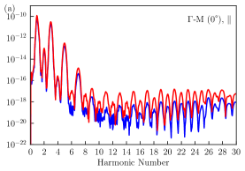
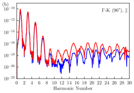
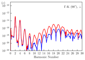
Figure 5: High harmonic generation spectrum computed for a single monolayer of hBN for the effective model (blue lines) and for the ab-initio model (red lines). (a,b,c) Harmonic spectrum for a laser pulse in the $\Gamma-\mathrm{M}$ ($\Gamma-\mathrm{K}$,$\Gamma-\mathrm{K}$) direction along its parallel (parallel, perpendicular) direction, respectively.

In Fig. 5, it is shown the spectrum for different pulse directions and different directions of emission. Symmetry imposes that for the $\Gamma-\mathrm{M}$ direction of the laser pulse the perpendicular current is strictly zero and for that reason is not shown. On the other hand, for the parallel emission, both even and odd harmonics are allowed due to the breaking of the inversion symmetry. When the laser pulse is aligned along the $\Gamma-\mathrm{K}$ direction, symmetry restricts harmonic emission to odd (even) harmonics for the parallel (perpendicular) emission (You et al., 2017). It is clear that first order harmonics, that are generated mostly by intraband current (Vampa et al., 2014), have an exponential decay until harmonic 13, that corresponds approximately to the bandgap energy, $5.62$ eV. It can be observed that the agreement between both models is extremely good given the simplicity of the effective model. For intraband harmonics the agreement between both approaches is almost quantitatively and for harmonics higher than the bandgap energy, usually coming from interband polarizations, the results agree on the overall shape having a discrepancy in its absolute value.

The quantitative discrepancy in the region of interband harmonics arises due to the approximation done in the construction of the dipole operator in the effective model. The assumption made in Eq. (III.1) for the effective model strongly reduces the possibility of recombination between distant Wannier orbitals and this can be observed by looking at the suppression of high harmonics when comparing against the ab-initio model. Furthermore, the low order harmonics have a much better agreement since it is not expected that recombination elements have a strong influence on them, just like Brunel harmonics in atomic HHG.

Conclusion

The Wannier gauge is presented in this work as a way to avoid the problem of random phases of the dipole couplings along the FBZ. The dynamical equations for the RDM are derived in the Wannier gauge. The presented formalism can provide a new framework in which DFT calculations and simple tight-binding Hamiltonians can be used for the description of the HHG process. The harmonic spectrum for a single monolayer of hBN is calculated and the results validate the use of the simplest tight-binding Hamiltonian commonly used (Neto et al., 2009) to study HHG when compared to ab-initio DFT calculations. Our work opens the window for the calculation of nonlinear optical response in crystals by using parameters directly extracted from ab-initio calculations using the MLWF procedure, that up to now was a cumbersome task due to the problem of the random phases in the dipole couplings.