Numerical study in stochastic homogenization for elliptic PDEs: convergence rate in the size of representative volume elements

Abstract

We describe the numerical scheme for the discretization and solution of 2D elliptic equations with strongly varying piecewise constant coefficients arising in the stochastic homogenization of multiscale composite materials. An efficient stiffness matrix generation scheme based on assembling the local Kronecker product matrices is introduced. The resulting large linear systems of equations are solved by the preconditioned CG iteration with a convergence rate that is independent of the grid size and the variation in jumping coefficients (contrast). Using this solver we numerically investigate the convergence of the Representative Volume Element (RVE) method in stochastic homogenization that extracts the effective behavior of the random coefficient field. Our numerical experiments confirm the asymptotic convergence rate of systematic error and standard deviation in the size of RVE rigorously established in [6]. The asymptotic behavior of covariances of the homogenized matrix in the form of a quartic tensor is also studied numerically. Our approach allows laptop computation of sufficiently large number of stochastic realizations even for large sizes of the RVE.

Key words: Stochastic homogenization, Representative Volume Element, elliptic problem solver, PCG iteration, homogenized matrix, empirical variance, Kronecker product, covariance of homogenization matrix.

AMS Subject Classification: 65F30, 65F50, 65N35, 65F10

1 Introduction

Homogenization methods allow to derive the effective mechanical and physical properties of highly heterogeneous materials from the knowledge of the spatial distribution of their components [1, 11]. In particular, stochastic homogenization via the Representative Volume Element (RVE) methods provide means for calculating the effective large-scale characteristics related to structural and geometric properties of random composites, by utilizing a possibly large number of probabilistic realizations [8, 9, 10, 6, 5]. The numerical investigation of the effective characteristics of random structures is a challenging problem since the underlying elliptic equation with randomly generated coefficients should be solved for many thousands realizations and for domains with substantial structural complexity to obtain sufficient statistics. Note that for every realization of the random medium one should construct a new stiffness matrix and right hand side to solve the discretized problem. Therefore, construction of fast solvers (which allow to confirm numerically the quantitative results in the stochastic homogenization) using the conventional computing facilities is a challenge.

This paper presents the numerical study of the stochastic homogenization of an elliptic system with randomly generated coefficients. Our approach is based on the FEM-Galerkin approximation of the 2D elliptic equations in a periodic setting by using fast assembling of the FEM stiffness matrix in a sparse matrix format, which is performed by agglomerating the Kronecker tensor products of simple 1D FEM discrete operators [12]. We use the product piecewise linear finite elements on the rectangular grid assuming that strongly varying piecewise constant equation coefficients are resolved on that grid. This scheme provides efficient approximation of equations with complicated jumping coefficients. The numerical analysis of the error in the Galerkin FEM approximation indicates the convergence rate $O(h^{\beta})$ in the $L^{2}$-norm with $3/2\leq\beta\leq 2$.

The resulting large linear system of equations is solved by the preconditioned CG iteration, where the convergence rate is proven to be independent on the grid size and the relative variation in jumping coefficients, i.e., on the contrast. The preconditioned iterative solvers for the discrete elliptic systems of equations with variable coefficients have been long since in the focus in the literature on numerical methods for multi-dimensional and stochastic PDEs, see [13, 14, 16] and the literature therein.

In this paper, we consider an ensemble of two-valued random coefficient fields, which is based on independently and uniformly placed (and thus overlapping) axi-parallel square inclusions of fixed side length. We investigate the RVE method that (approximately) extracts the effective (i.e. large-scale) behavior of the medium in form of the deterministic and homogeneous matrix $\mathbb{A}_{hom}$ from a given (stationary and ergodic) ensemble. This method produces an approximation to $\mathbb{A}_{hom}$ by solving $D=2$ elliptic equations on a torus of (lateral) size $L$ with a specific right hand side (the corrector equation), by taking the spatial average of the flux of these solutions, and by taking the empirical mean over $N$ independent realizations of this coefficient field under the naturally periodized version of the ensemble. This is an approximation in so far as the outcome is still random (as quantified by the standard deviation of the outcome of a single realization) and that the periodic boundary conditions affect the statistics (which we call the systematic error). In [6], Gloria, Neukamm and the last author rigorously derived upper bounds how the standard deviation and the systematic error decrease with increasing RVE size $L$. Our numerical experiments confirm the scaling of these bounds. Since numerically, there is no access to exact values of the variance (or standard expectation) or the expectation, we replace these quantities by their empirical counterparts for a large number of realizations $N$. We thus first provide numerical evidence that these quantities have saturated in $N$, and second that their limiting values display the predicted scaling in $L$.

In work [4] by Duerinckx, Gloria and the last author, it was worked out that the properly rescaled variance of the output of the RVE converges as $L\uparrow\infty$ to a quartic tensor $Q$ that governs the leading-order fluctuations of any solution. In this paper, we show how the symmetry properties of the ensemble yields symmetry properties of $Q$ (and its approximation). Also, a convergence rate was rigorously established in that work, and is being numerically investigated here. While the number of samples $N$ considered here seems too low to reach saturation in the empirical variance, the findings are at least not in contradiction with the theoretic results.

In numerical tests on the stochastic properties of the 2D RVE method we study the asymptotics of empirical variance versus the size of RVE $L\leq 128$, and of the systematic error versus the number of realizations $N$ up to $N=10^{5}$. Furthermore, we estimate the convergence of the quartic tensor by implementing a large number of stochastic realizations. The proposed techniques allow to compute a sufficiently large number of realizations of random coefficient fields with a large number of overlapping inclusions up to $L^{2}=128^{2}$ corresponding to the stiffness matrix size $513^{2}\times 513^{2}$ using MATLAB on a moderate computer cluster.

The numerical investigation of the stochastic homogenization problem attracts interest and becomes an active field of research, see the survey [1] and references therein. Recently the numerical solution of the corrector-type problem, in the context of homogenization of the diffusion equation with spherical inclusions by using boundary element methods and the fast multipole techniques has been considered in [3].

The rest of the paper is organized as follows. In Section 2, we address the problem setting and define the elliptic equations of stochastic homogenization. Section 3 describes the Galerkin-FEM discretization scheme based on the fast matrix generation by using sums of Kronecker products of single-dimensional matrices. We also outline the PCG iteration applied in the computer simulations and provide numerics on the FEM discretization error. Section 4 introduces the computational scheme for the stochastic average coefficient matrix. Furthermore, in Section 4.3 we describe the construction and properties of the covariances of the homogenized matrix in the form of a quartics tensor. Section 5 presents results of numerical experiments on the empirical average and systematic error at the limit of a large number of stochastic realizations. The asymptotic of the quartic tensor versus the leading order variances is analyzed numerically in Section 5.2. Conclusions outline the main results of the paper. In Appendix the spectral properties of the discrete stochastic elliptic operators are studied numerically for a sequence of stochastic realizations.

2 Elliptic equations in stochastic homogenization

In this section, we describe the problem setting in the stochastic homogenization theory. For given $f\in{\cal L}^{2}(\Omega)$ such that $\int_{\Omega}f(x)dx=0$, we consider the class of model elliptic boundary value problems on the $d$-dimensional torus $\Omega:=[0,L)^{d}$ of side-length $L\in\mathbb{N}$: find $\phi\in H^{1}(\Omega)$, s.t.

$${\cal A}\phi:=-\nabla\cdot\mathbb{A}(x)\nabla\phi=f(x),\quad x=(x_{1},\ldots,x_{d})\in\Omega,$$ (2.1)

with the diagonal $d\times d$ uniformly elliptic coefficient matrix $\mathbb{A}(x)$, $\infty>\beta_{0}I\geq\mathbb{A}(x)\geq\alpha_{0}I>0$. In this paper we focus on the special class of elliptic problems (2.1) arising in stochastic homogenization theory where the highly varying coefficient matrix and the right-hand side are defined by a sequence of stochastic realizations as described in [8, 9, 10, 6, 5], see details in Sections 3 and 4.

In what follows, we present the numerical analysis for 2D stochastic homogenization problems (2.1) with periodic boundary conditions on $\Gamma=\partial\Omega$, in the form

$$\phi(0,x_{2})=\phi(L,x_{2}),\quad\frac{\partial}{\partial x_{1}}\phi(0,x_{2})=\frac{\partial}{\partial x_{1}}\phi(L,x_{2}),\quad x_{2}\in[0,L),$$

$$\phi(x_{1},0)=\phi(x_{1},L),\quad\frac{\partial}{\partial x_{2}}\phi(x_{1},0)=\frac{\partial}{\partial x_{2}}\phi(x_{1},L),\quad x_{1}\in[0,L).$$

The diagonal $2\times 2$ coefficient matrix $\mathbb{A}(x)$ is defined by

$$\mathbb{A}(x)=\begin{pmatrix}a(x)&0\\ 0&a(x)\\ \end{pmatrix},\quad\quad x\in\Omega,$$

where the scalar function $a(x)>0$ is piecewise constant in $\Omega$. The efficient numerical simulation pre-supposes the fast numerical solution of the equation (2.1) in the case of many different coefficients $\mathbb{A}(x)$ and right-hand sides, generated by certain stochastic procedure, and in the calculation of various functionals on the sequence of solutions $\phi$. In this problem setting the bottleneck task is fast and accurate generation of the FEM stiffness matrix in the sparse matrix form, which should be re-calculated many hundred if not thousand times in the course of stochastic realizations.

In asymptotic analysis of stochastic homogenization problems the coefficient and the right-hand side are chosen in a specific way, see [10, 8] for the particular problem setting. In this paper, we describe the conventional 2D FEM discretization scheme in the rescaled domain $\Omega=[0,1)^{2}$. Given the size of representative volume elements $L=1,2,3,\ldots$ we generate (possibly overlapping) decomposition of the domain $\Omega$ into $L^{2}$ equal unit cells $G_{s}$, $s=1,\ldots,L^{2}$, each of size $\frac{2\alpha}{L}\times\frac{2\alpha}{L}$, whose centers are distributed randomly (by the Poisson distribution) within the supercell $\Omega$, taking into account periodicity in both spacial variables $x_{1}$ and $x_{2}$. Here the overlap factor satisfies $\alpha\leq 1/2$. Stochastic characteristics of the system can be estimated at the limit of a large number $L$.

We consider a sequence of random coefficient distributions $\{G_{s}\}_{n}$, numbered by $n=1,\ldots,N$, where the particular set $\{G_{s}\}=\{G_{s}\}_{n}$ for fixed $n$ will be called a realization. For any fixed realization define the covered domain

$$\widehat{G}=\widehat{G}_{n}:=\bigcup^{L^{2}}_{s=1}G_{s},$$ (2.2)

and the respective coefficient

$$\widehat{a}(x)=\widehat{a}^{(n)}(x)=\left\{\begin{array}[]{ll}1&\mbox{if }x\in\widehat{G}_{n},\\ 0&\mbox{otherwise}.\end{array}\right.$$ (2.3)

The stochastic model is specified by the choice of the overlap constant $\alpha\in(0,1/2]$ and the scaling factor $\lambda\in(0,1]$. In the following, the constant $\lambda$ will be fixed in the interval $0.1\leq\lambda\leq 0.8$. We denote the “stochastic” elliptic operator for the particular realization by ${\cal A}^{(n)}={\cal A}_{\lambda}^{(n)}$ or just ${\cal A}$ (if $n$ is fixed) so that

$${\cal A}^{(n)}=-\nabla\cdot\mathbb{A}^{(n)}(x)\nabla,$$

where the corresponding $2\times 2$ coefficient matrix $\mathbb{A}^{(n)}(x)$ is defined by

$$\mathbb{A}^{(n)}(x)=\lambda\begin{pmatrix}1&0\\ 0&1\\ \end{pmatrix}+(1-\lambda)\begin{pmatrix}\widehat{a}^{(n)}(x)&0\\ 0&\widehat{a}^{(n)}(x)\\ \end{pmatrix}:=\begin{pmatrix}{a}^{(n)}(x)&0\\ 0&{a}^{(n)}(x)\\ \end{pmatrix},\quad x\in\Omega,$$ (2.4)

and the diagonal matrix coefficient takes the form

$${a}^{(n)}(x)=\lambda+(1-\lambda)\widehat{a}^{(n)}(x).$$ (2.5)

We use the notation $\widehat{\mathbb{A}}^{(n)}(x)$ for the ”stochastic part” of a matrix associated with the diagonal coefficient $\widehat{a}^{(n)}(x)$, i.e.

$$\widehat{\mathbb{A}}^{(n)}(x)=\begin{pmatrix}\widehat{a}^{(n)}(x)&0\\ 0&\widehat{a}^{(n)}(x)\\ \end{pmatrix}.$$

Now the elliptic equations in stochastic homogenization are formulated as follows. Fixed coefficient $\widehat{\mathbb{A}}^{(n)}(x)$, for $i=1,2$ solve the periodic elliptic problems in $\Omega$,

$$-\lambda\Delta\phi_{i}-(1-\lambda)\nabla\cdot\widehat{\mathbb{A}}^{(n)}({\bf e}_{i}+\nabla\phi_{i})=0,$$ (2.6)

where the directional unit vectors ${\bf e}_{i}$, $i=1,2$, are given by ${\bf e}_{1}=(1,0)^{T}$ and ${\bf e}_{2}=(0,1)^{T}$, see Section 4 for more details. The variational form of the equation (2.6) reads as follows

$$\int_{\Omega}(\lambda\nabla\phi_{i}\cdot\nabla\psi+(1-\lambda)\widehat{a}^{(n)}(x)[{\bf e}_{i}+\nabla\phi_{i}]\cdot\nabla\psi)dx=0\quad\forall\;\psi\in H^{1}(\Omega).$$ (2.7)

The equation (2.6) can be also written in the classical form (2.1)

$${\cal A}^{(n)}\phi_{i}=f_{i},\quad\mbox{with}\quad f_{i}=(1-\lambda)\nabla\cdot\widehat{a}^{(n)}\,{\bf e}_{i}.$$ (2.8)

Fig. 2.1 illustrates an example of the particular realization of stochastic coefficient $a^{(n)}(x)$ in the case $L=8$, $\lambda=0.1$ and $\alpha=1/4$ visualized on $m_{1}\times m_{1}$ grid with $m_{1}=97$.

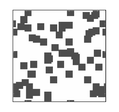
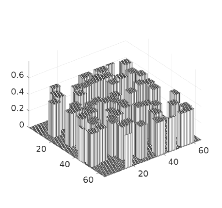
Figure 2.1: A realization of a stochastic process with $L^{2}$ overlapping cells for $L=8$, $\alpha=1/4$.

The problem setting remains verbatim in the $d$-dimensional case, $d>2$. In this case the equation (2.8) takes the same form, where a $d\times d$ coefficient matrix is given by

$$\mathbb{A}^{(n)}(x)=\mbox{diag}\{a^{(n)}(x),\ldots,a^{(n)}(x)\},\quad x\in\Omega$$

and ${\bf e}_{i}\in\mathbb{R}^{d}$, $i=1,\ldots,d$, represent the set of directional unit vectors in $\mathbb{R}^{d}$.

3 Matrix generation and iterative solution

In this section we describe the FEM discretization scheme and the fast matrix generation approach based on the use of tensor Kronecker products of “univariate” matrices.

3.1 Galerkin FEM discretization

First, we introduce the uniform $m_{s}\times m_{s}$ rectangular grid $\Omega_{h_{s}}$ in $\Omega$ with the grid size $h_{s}=\frac{1}{m_{s}-1}$, such that $m_{s}=m_{0}L+1$, $m_{0}=2^{p_{0}}$, i.e. $h_{s}=\frac{1}{m_{0}L}$. We assume that the unit cell $G_{s}$, $s=1,\ldots L^{2}$, of size $\frac{2\alpha}{L}\times\frac{2\alpha}{L}$ adjust the square grid $\Omega_{h_{s}}$, such that the center $c_{s}$ of $G_{s}$ belongs to the set of grid points in $\Omega_{s}$, while the overlap factor $\alpha$ may take values $\alpha\in\{\frac{1}{m_{0}},\frac{2}{m_{0}},\ldots\frac{2^{p_{0}-1}}{m_{0}}\}$. In this construction the univariate size of the unit cell varies as

$$\frac{2\alpha}{L}=\frac{2\alpha m_{0}}{m_{0}L}=kh_{s},\quad\mbox{with }\quad k=2,\;4,\;\ldots m_{0}.$$

In the following numerical examples we normally use the overlap constant $\alpha=1/4$. For $\alpha=1/2$, the maximal size of the unit cell is given by $\frac{1}{L}\times\frac{1}{L}$, which contains $m_{0}+1$ grid points in each spacial direction leading to $m_{1}\times m_{1}$ rectangular grid with $m_{1}=m_{0}L+1$.

The FEM discretization of the elliptic PDE in (2.8) can be constructed, in general, on the finer grid $\Omega_{h}$ compared with $\Omega_{s}$, which serves for the resolution of jumping coefficients. To that end, we introduce the $m_{1}\times m_{1}$ rectangular grid $\Omega_{h}$ with the mesh size $h=\frac{1}{m_{1}-1}$, $m_{1}\geq m_{s}$, that is obtained by a dyadic refinement of the grid $\Omega_{s}$, such that the relation

$$m_{1}-1=(m_{s}-1)2^{p},\quad\mbox{with}\quad p=0,1,2,\ldots$$ (3.1)

holds, implying $h_{s}=2^{p}h$. Now the grid-size of the unit cell $G_{s}$ on the finer grid $\Omega_{h}$ is given by $(m_{0}2^{p}+1)\times(m_{0}2^{p}+1)$.

Given a finite dimensional space $X\subset H^{1}(\Omega)$ of tensor product piecewise linear finite elements $X=\mbox{span}\{\psi_{\mu}(x)\}$ associated with the grid $\Omega_{h}$, with $\mu=1,...,M_{d}$, $M_{d}=m_{1}^{d}$, for $d=2$ incorporating periodic boundary conditions, we are looking for the traditional FEM Galerkin approximation of the exact solution in the form

$$\phi(x)\approx\phi_{X}(x)=\sum_{\mu=1}^{M_{d}}u_{\mu}\psi_{\mu}(x)\in X,$$

where ${\bf u}=(u_{1},\ldots,u_{M_{d}})^{T}\in\mathbb{R}^{M_{d}}$ is the unknown coefficients vector. Fixed realization of the coefficient $a^{(n)}(x)$, for $i=1,2$ we define the Galerkin-FEM discretization with respect to $X$ of the variational equation (2.7) by

$$A{\bf u}_{i}={\bf f}_{i},\quad A=[a_{\mu\nu}]\in\mathbb{R}^{M_{d}\times M_{d}},\quad{\bf f}_{i}={\bf f}=[f_{\mu}]\in\mathbb{R}^{M_{d}},$$ (3.2)

where the Galerkin-FEM matrix $A$ generated by the equation coefficient ${\mathbb{A}}^{(n)}(x)$ is calculated by using the associated bilinear form

$$a_{\mu\nu}=\langle{\cal A}\psi_{\mu},\psi_{\nu}\rangle=\int_{\Omega}(\lambda\nabla\psi_{\mu}\cdot\nabla\psi_{\nu}+(1-\lambda)a^{(n)}(x)\nabla\psi_{\mu}\cdot\nabla\psi_{\nu})dx,$$ (3.3)

and

$$f_{\mu}=\langle f,\psi_{\mu}\rangle=\int_{\Omega}(1-\lambda)\nabla\cdot\widehat{a}^{(n)}(x)\,{\bf e}_{i}\psi_{\mu}\,dx=-(1-\lambda)\int_{\Omega}\widehat{a}^{(n)}(x)\frac{\partial\psi_{\mu}}{\partial x_{i}}dx.$$ (3.4)

Corresponding to (2.8) and (3.3), we represent the stiffness matrix $A$ in the additive form

$$A=\lambda A_{\Delta}+(1-\lambda)\widehat{A}_{s},$$ (3.5)

where $A_{\Delta}$ represents the $M_{d}\times M_{d}$ FEM Laplacian matrix in periodic setting that has the standard two-terms Kronecker product form. Here matrix $\widehat{A}_{s}$ provides the FEM approximation to the ”stochastic part” in the elliptic operator corresponding to the coefficient $\widehat{a}^{(n)}(x)$, see (2.4). The latter is determined by the sequence of random coefficients distribution in the course of stochastic realizations, numbered by $n=1,\ldots,N$.

In the case of complicated jumping coefficients the stiffness matrix generation in the elliptic FEM usually constitutes the dominating part of the overall solution cost. In the course of stochastic realizations the equation (3.2) is to be solved many hundred or even thousand times, so that every time one has to update the stiffness matrix $A$ and the right-hand side $\bf f$.

Our discretization scheme computes all matrix entries at the low cost by assembling of the local Kronecker product matrices obtained by representation of $\widehat{a}^{(n)}(x)$ as a sum of separable functions. This allows to store the resultant stiffness matrix in the sparse matrix format. Such a construction only includes the pre-computing of tri-diagonal matrices representing 1D elliptic operators with jumping coefficients in periodic setting. In the next sections, we shall describe the efficient construction of the ”stochastic” term $A_{s}$.

3.2 Matrix generation by using Kronecker product sums

To enhance the time consuming matrix assembling process we apply the FEM Galerkin discretization (3.3) of equation (2.8) by means of the tensor-product piecewise linear finite elements

$$\{\psi_{\boldsymbol{\mu}}(x):=\psi_{\mu_{1}}(x_{1})\cdots\psi_{\mu_{d}}(x_{d})\},\quad{\boldsymbol{\mu}}=(\mu_{1},\ldots,\mu_{d}),\quad\mu_{\ell}\in{\mathcal{I}}_{\ell}=\{1,\ldots,m_{\ell}\},\;\ell=1,\ldots,d,$$

where $\psi_{\mu_{\ell}}(x_{\ell})$ are the univariate piecewise linear hat functions. The $M_{d}\times M_{d}$ stiffness matrix is constructed by the standard mapping of the multi-index $\boldsymbol{\mu}$ into the long univariate index $1\leq\mu\leq M_{d}$ for the active degrees of freedom in periodic setting. For instance, we use the so-called big-endian convention for $d=3$ and $d=2$

$${\boldsymbol{\mu}}\mapsto\mu:=\mu_{3}+(\mu_{2}-1)m_{3}+(\mu_{1}-1)m_{2}m_{3},\quad{\boldsymbol{\mu}}\mapsto\mu:=\mu_{2}+(\mu_{1}-1)m_{2},$$

respectively. In what follows, we consider the case $d=2$ in more detail.

In our discretization scheme we calculate the stiffness matrix by assembling of the local Kronecker product terms by using representation of the “stochastic part” in the coefficient $\widehat{a}^{(n)}(x)$ as an $R$-term sum of separable functions. To that end, let us assume for the moment that the scalar diffusion coefficient $a(x_{1},x_{2})$ can be represented in the separate form (rank-$1$ representation)

$$a(x_{1},x_{2})=a^{(1)}(x_{1})a^{(2)}(x_{2}).$$

Then the entries of the Galerkin stiffness matrix $A=[a_{{\mu}{\nu}}]\in\mathbb{R}^{M_{d}\times M_{d}}$ can be represented by

$$a_{{\mu}{\nu}} =\langle{\mathcal{A}}\psi_{\mu},\psi_{\nu}\rangle=\int_{\Omega}a^{(1)}(x_{1})a^{(2)}(x_{2})\nabla\psi_{\mu}\cdot\nabla\psi_{\nu}dx$$

$$={\int_{(0,1)}}a^{(1)}(x_{1})\dfrac{\partial\psi_{\mu_{1}}(x_{1})}{\partial x_{1}}\dfrac{\partial\psi_{\nu_{1}}(x_{1})}{\partial x_{1}}dx_{1}\int_{(0,1)}a^{(2)}(x_{2})\psi_{\mu_{2}}(x_{2})\psi_{\nu_{2}}(x_{2})dx_{2}$$

$$+\int_{(0,1)}a^{(1)}(x_{1})\psi_{\mu_{1}}(x_{1})\psi_{\nu_{1}}(x_{1})dx_{1}\int_{(0,1)}a^{(2)}(x_{2})\dfrac{\partial\psi_{\mu_{2}}(x_{2})}{\partial x_{2}}\dfrac{\partial\psi_{\nu_{2}}(x_{2})}{\partial x_{2}}dx_{2},$$

which leads to the rank-2 Kronecker product representation

$${A}={A}_{1}\otimes S_{2}+S_{1}\otimes{A}_{2},$$

where $\otimes$ denotes the conventional Kronecker product of matrices, see Definition 3.1 below. Here ${A}_{1}=[a_{\mu_{1}\nu_{1}}]\in\mathbb{R}^{m_{1}\times m_{1}}$ and ${A}_{2}=[a_{\mu_{2}\nu_{2}}]\in\mathbb{R}^{m_{2}\times m_{2}}$ denote the univariate stiffness matrices and $S_{1}=[s_{\mu_{1}\nu_{1}}]\in\mathbb{R}^{m_{1}\times m_{1}}$ and $S_{2}=[s_{\mu_{2}\nu_{2}}]\in\mathbb{R}^{m_{2}\times m_{2}}$ define the weighted mass matrices, for example

$$a_{\mu_{1}\nu_{1}}={\int_{(0,1)}}a^{(1)}(x_{1})\frac{\partial\psi_{\mu_{1}}(x_{1})}{\partial x_{1}}\frac{\partial\psi_{\nu_{1}}(x_{1})}{\partial x_{1}}dx_{1},\quad s_{\mu_{1}\nu_{1}}=\int_{(0,1)}a^{(1)}(x_{1})\psi_{\mu_{1}}(x_{1})\psi_{\nu_{1}}(x_{1})dx_{1}.$$

Definition 3.1

Recall that given $p_{1}\times q_{1}$ matrix $A$ and $p_{2}\times q_{2}$ matrix $B$, their Kronecker product is defined as a $p_{1}p_{2}\times q_{1}q_{2}$ matrix $C$ via the block representation

$$C=A\otimes B=[a_{ij}B],\quad i=1,\ldots,p_{1},\;j=1,\ldots,q_{1}.$$

Let us discuss in more detail the calculation of the 1D stiffness matrices $A_{1}$ and $A_{2}$ in the case of variable 1D coefficients. We choose the Galerkin FEM with $m=m_{1}$ piecewise-linear hat functions $\left\{\psi_{\mu_{1}}\right\}$ in periodic setting in $\Omega=[0,1)$, constructed on a uniform grid with a step size $h=1/m$, and nodes $x_{\mu_{1}}=h\,{\mu_{1}}$, ${\mu_{1}}=1,\ldots,m$. If we denote the diffusion coefficient by $a(x_{1})$, then the entries of the exact stiffness matrix ${A}_{1}$ read as

$$\left(a\right)_{\mu_{1},\mu_{1}^{\prime}}=\langle a(x)\nabla\psi_{\mu_{1}}(x),\nabla\psi_{\mu_{1}^{\prime}}(x)\rangle_{L_{2}(D)},\quad{\mu_{1}},{\mu_{1}^{\prime}}=1,\ldots,m.$$

We assume that the coefficient remains constant at each spatial interval $[x_{\mu_{1}-1},x_{\mu_{1}}]$, which corresponds to the evaluation of the scalar product above via the midpoint quadrature rule yielding the approximation order $O({h^{2}})$.

Introducing the coefficient vector ${\bf a}=[a_{\mu_{1}}]\in\mathbb{R}^{m}$, $a_{\mu_{1}}=a(x_{\mu_{1}-1/2})$, $\mu_{1}=1,\ldots,m$, where $x_{i_{1}-1/2}$ is the middle point of the integration interval, the symmetric tridiagonal matrix of interest can be represented by

$${A}_{1}=\dfrac{1}{h}\left[\begin{matrix}a_{1}+a_{2}&-a_{2}&&&-a_{1}\\ -a_{2}&a_{2}+a_{3}&-a_{3}\\ &\ddots&\ddots&\ddots\\ &&-a_{m-1}&a_{m-1}+a_{m}&-a_{m}\\ -a_{1}&&&-a_{m}&a_{m}+a_{1}\end{matrix}\right].$$ (3.6)

By simple algebraic transformations (e.g. by lamping of the mass matrices) the matrix ${A}$ can be simplified to the form (without loss of approximation order)

$${A}\mapsto A=A_{1}\otimes D_{2}+D_{1}\otimes A_{2},$$ (3.7)

where $D_{1},D_{2}$ are the diagonal matrices with positive entries. This representation applies in particular to the periodic Laplacian.

In the general case, the piecewise constant stochastic coefficient can be represented as an $R$-term sum of separable coefficients. This leads to the linear system of equations

$$A{\bf u}={\bf f},$$ (3.8)

constructed for the general $R$-term separable coefficient $a(x_{1},x_{2})$ with $R>1$.

The representation in (3.7) can be further simplified to the anisotropic Laplacian type matrix

$${A}\mapsto B=\alpha_{2}A_{1}\otimes I_{2}+\alpha_{1}I_{1}\otimes A_{2},$$

which will be used as a prototype preconditioner for solving the target linear system (3.8).

Taking into account the rectangular structure of the grid, we use the simple finite-difference (FD) scheme for the matrix representation of the Laplacian operator $-\Delta$. In this case the scaled discrete Laplacian incorporating periodic boundary conditions takes the form

$$A_{\Delta}=\Delta_{1}\otimes I_{m_{2}}+I_{m_{1}}\otimes\Delta_{2},$$ (3.9)

where

$$-\Delta_{1}=\mathrm{tridiag}\{1,-2,1\}+P^{(1)}\in\mathbb{R}^{m_{1}\times m_{1}},$$

such that the entries of the ”periodization” matrix $P^{(1)}\in\mathbb{R}^{m_{1}\times m_{1}}$ are all zeros except

$$P^{(1)}_{1,m_{1}}=P^{(1)}_{m_{1},1}=1,\quad\mbox{and}\quad P^{(1)}_{1,1}=P^{(1)}_{m_{1},m_{1}}=-1.$$

Here $I_{m_{1}}\in\mathbb{R}^{m_{1}\times m_{1}}$ is the identity matrix, $\Delta_{1}=\Delta_{2}$ is the 1D finite difference Laplacian (endorsed with the Neumann boundary conditions), and $\otimes$ denotes the Kronecker product of matrices, see Definition 3.1. We say that the Kronecker rank of both $A$ in (3.7) and $A_{\Delta}$ in (3.9) equals to $2$.

Notice that the $m_{1}\times m_{1}$ Laplacian matrices for the Neumann and periodic boundary conditions in 1D read as

$$\Delta_{N}=\begin{bmatrix}-1&1&\cdots&0&0\\ 1&-2&\cdots&0&0\\ \vdots&\vdots&\ddots&\vdots&\vdots\\ 0&0&\cdots&-2&1\\ 0&0&\cdots&1&-1\\ \end{bmatrix}\quad\mbox{ and }\quad\Delta_{P}=\begin{bmatrix}-2&1&\cdots&0&1\\ 1&-2&\cdots&0&0\\ \vdots&\vdots&\ddots&\vdots&\vdots\\ 0&0&\cdots&-2&1\\ 1&0&\cdots&1&-2\\ \end{bmatrix},$$ (3.10)

respectively.

In the $d$-dimensional case we have the similar Kronecker rank-$d$ representations. For example, in the case $d=3$ the ”periodic” Laplacian $M_{d}\times M_{d}$ matrix $A_{\Delta}$ takes a form

$$A_{\Delta}=A_{1,P}\otimes I_{2}\otimes I_{3}+I_{1}\otimes A_{2,P}\otimes I_{3}+I_{1}\otimes I_{2}\otimes A_{3,P},$$

such that its Kronecker rank equals to $3$, and similar for the arbitrary $d\geq 3$.

3.3 Fast matrix assembling for the stochastic part

The Kronecker form representation of the ”stochastic” term in (3.3) further denoted by $A_{s}$ is more involved. For given stochastically chosen distribution of overlapping cells $G_{s}$, $s=1,\ldots,L^{2}$, we construct the minimal non-overlapping decomposition of the full covered grid domain $\widehat{G}=\cup^{L^{2}}_{s=1}G_{s}$ colored by gray in Figure 2.1 (we have $a(x)=1$ for $x\in\widehat{G}$ and $a(x)=\lambda$ for $x\in\Omega\setminus\widehat{G}$) in a form of a union of elementary square cells $S_{k}$, $k=1,\ldots,K$, $K\geq L^{2}$, each of the grid-size $\overline{m}_{0}\times\overline{m}_{0}$,

$$\widehat{G}=\cup^{K}_{k=1}S_{k}.$$ (3.11)

Here $\overline{m}_{0}=2^{p}+1$, and $p=0,1,2,\ldots$, is fixed as above by relation $m_{1}-1=(m_{s}-1)2^{p}$. In this construction, the non-overlapping elementary cells $S_{k}$ for different $k$ are allowed to have the only common edges of size $\overline{m}_{0}$. Notice that in the case of non-overlapping decomposition (2.2) the set of cells $\{S_{k}\}$ coincides with the initial set $\{G_{s}\}$ which allows to maximize the size $\overline{m}_{0}\times\overline{m}_{0}$ of each $S_{k}$, $k=1,\ldots,L^{2}$, to the largest possible, i.e. to $\overline{m}_{0}=m_{0}2^{p}+1$.

To finalize the matrix generation procedure for $A_{s}$, we define the local $\overline{m}_{0}\times\overline{m}_{0}$ matrices representing the discrete Laplacian with Neumann boundary conditions,

$$\widehat{Q}_{\overline{m}_{0}}:=\mbox{tridiag}\{1,-2,1\}+\mbox{diag}\{1,0,\ldots,0,1\}\in\mathbb{R}^{\overline{m}_{0}\times\overline{m}_{0}},$$

and the diagonal matrix

$$\widehat{I}_{\overline{m}_{0}}:=\mbox{diag}\{1/2,1,\ldots,1,1/2\}\in\mathbb{R}^{\overline{m}_{0}\times\overline{m}_{0}},$$

see the visualization in (3.10). Here, we may select $\overline{m}_{0}=2,3,5,...$ that corresponds to the choice $p=0,1,2,...$. In the case of $\overline{m}_{0}\times\overline{m}_{0}$ matrix with minimal size $\overline{m}_{0}=2$, both discrete Laplacians in (3.10) simplify to

$$\Delta_{N}=\begin{bmatrix}-1&1\\ 1&-1\\ \end{bmatrix}\quad\mbox{ and }\quad\Delta_{P}=\begin{bmatrix}-1&1\\ 1&-1\\ \end{bmatrix}.$$ (3.12)

Let the subdomain $S_{k}$ be supported by the index set $I_{k}^{(1)}\times I_{k}^{(2)}$ of size $\overline{m}_{0}\times\overline{m}_{0}$ for $k=1,\ldots,K$. Introduce the block-diagonal matrices $\overline{Q}_{k}\in\mathbb{R}^{m_{1}\times m_{1}}$ and $\overline{I}_{k}\in\mathbb{R}^{m_{1}\times m_{1}}$ by inserting matrices $\widehat{Q}_{\overline{m}_{0}}$ and $\widehat{I}_{\overline{m}_{0}}$ as diagonal blocks into $m_{1}\times m_{1}$ zero matrix in the positions $I_{k}^{(1)}\times I_{k}^{(1)}$ and $I_{k}^{(2)}\times I_{k}^{(2)}$, respectively.

Now the stiffness matrix $A_{s}$ is represented in the form of a Kronecker product sum as follows,

$$A_{s}=\sum^{K}_{k=1}(\overline{Q}_{k}\otimes\overline{I}_{k}+\overline{I}_{k}\otimes\overline{Q}_{k})+P^{(2)},$$ (3.13)

where

$$P^{(2)}=P^{(1)}\otimes I_{m_{1}}+I_{m_{1}}\otimes P^{(1)}\in\mathbb{R}^{M_{d}\times M_{d}}$$

is the ”periodization” matrix in 2D. In a $d$-dimensional case the representation (3.13) generalizes to a sum of $d$-factor Kronecker products

$$A_{s}=\sum^{K}_{k=1}(\overline{Q}_{k}\otimes\overline{I}_{k}\otimes\cdots\otimes\overline{I}_{k}+\ldots+\overline{I}_{k}\otimes\cdots\otimes\overline{I}_{k}\otimes\overline{Q}_{k})+P^{(d)},$$ (3.14)

where $P^{(d)}$ is the ”periodization” matrix in $d$ dimensions, constructed as the $d$-term Kronecker sum similar to the case $d=2$.

The Kronecker product form of (3.9) and (3.13) leads to the corresponding Kronecker sum representation for the total stiffness matrix $A$. This allows an efficient implementation of the matrix assembly and low storage for the stiffness matrix preserving the Kronecker sparsity. Hence, it proves the following storage complexity for the matrix $A$.

Lemma 3.2

The storage size for the stiffness matrix $A$ is bounded by

$$Stor(A)\approx Stor(A_{s})=O(d\overline{m}_{0}K+dm_{1}).$$

Here, in general, the number $K$ of elementary cells is larger than $L^{2}$, and it coincides with $L^{2}$ only in the case of non-overlapping decomposition $\widehat{G}=\cup^{L^{2}}_{s=1}G_{s}$, where different patches $G_{s}$ are allowed to have joint pieces of boundary but no overlapping area.

In the general case $d\geq 2$ and $K\geq L^{d}$, the Kronecker rank of the matrix ${A}$ is bounded by

$$\mbox{rank}_{Kron}({A})\leq d\,K.$$

The Kronecker rank of the stiffness matrix reduces dramatically in two cases:
(a) For the case of non-overlapping cells $G_{s}$, $s=1,\ldots,L^{2}$, we have

$$\mbox{rank}_{Kron}({A})\leq L^{d}.$$

(b) In the case of cell-centered locations of subdomains $G_{s}$ (special case of geometric homogenization) there holds

$$\mbox{rank}_{Kron}({A})\leq L^{d-1}.$$

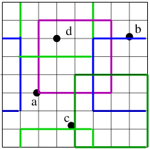
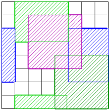
Figure 3.1: Example of the covering domain $\widehat{G}$ (right) and the typical locations of sampling points for the grid representation of $\mathbb{A}_{h}(x_{h})$ (left).

The corresponding vector representation ${\bf f}_{i}\in\mathbb{R}^{M_{d}}$ of the right hand side $f_{i}(x)$ is computed by multiplication of the discrete upwind gradient matrix $\nabla_{h}$ with a vector ${\bf y}_{i}\in\mathbb{R}^{M_{d}}$. Here the vector ${\bf y}_{i}$ represents the multiple of the vector ${\bf e}_{i}$, $i=1,2$, and the equation coefficient $\mathbb{A}^{(n)}=\mathbb{A}(x)=\mbox{diag}\{{a}^{(n)}(x),{a}^{(n)}(x)\}$, discretized on the grid $\Omega_{h}$, i.e. each block-entry of the ”discretized” matrix coefficient $\mathbb{A}(x)\mapsto A_{h}(x_{h})$ is given by an $M_{d}$-vector array with $M_{d}=m^{2}$,

$$A_{h}(x_{h})=\mbox{diag}\{{a}^{(n)}(x_{h}),{a}^{(n)}(x_{h})\},\quad{a}^{(n)}(x_{h})_{|x_{h}\in\Omega_{h}}\in\mathbb{R}^{M_{d}}.$$

Hence, we finally arrive at

$${\bf f}_{i}=(1-\lambda)\nabla_{h}\cdot{\bf y}_{i},\quad{\bf y}_{i}=[{\bf y}_{i}(x_{h})]\in\mathbb{R}^{M_{d}}\;\;\mbox{with}\;\;{\bf y}_{i}(x_{h})={A}_{h}(x_{h}){\bf e}_{i},\quad x_{h}\in\Omega_{h},$$

for $i=1,2$. Specifically, given the grid-point $x_{h}\in\Omega_{h}$, the corresponding diagonal value of ${A}_{h}(x_{h})$ is defined by $a^{(n)}(x_{h})$, see (2.5). Here the variable part $\widehat{a}^{(n)}(x_{h})$, describing the jumping coefficient, is assigned by $1$ for interior points in $\widehat{G}$, by $1/2$ for interface points (the angle equals to $\pi/2$), by $3/4$ for the ”interior” L-shaped corners (the angle equals to $3\pi/4$) and by $1/4$ for the ”exterior” corner of $\widehat{G}$ (the angle equals to $\pi/4$), see points (d), (b), (c) and (a) in Figure 3.1, respectively. This figure corresponds to $L=2$, the discretization parameter $n_{0}=4$ and periodic completion of the geometry. One observes the complicated shape of the strongly jumping coefficients.

3.4 Numerical analysis of the FEM approximation error

We tested convergence of the solutions on a sequence of dyadic refined grids, for the fixed configuration of coefficients and the right hand side given by $f=sin(2\pi x)cos(6\pi y)$. Test examples are performed for $L=2,\;4,\;8$, corresponding to $4$, $16$ and $64$ bumps in the coefficients, respectively. We compare the solution vectors ${\bf u}_{p}$ calculated on a sequence of five dyadic refined grids with the grid size $M_{d}=m_{p}^{2}=M_{d,p}$, with $m_{p}=2^{4+p}-1$, $p=1,\ldots,5$, equal to $M_{d,p}=31^{2}$, $63^{2}$, $127^{2}$, $255^{2}$, $511^{2}$ and $1023^{2}$, respectively. The matrix size is given by $M_{d}\times M_{d}$. A FEM interpolation error in the $H^{r}(\Omega)$-norm is expected of the order of $O(m^{-\beta+r})$ for $\beta\in(0,2]$ and $r\in[0,1]$, where $h=O(1/m)$ and $\beta$ measures the regularity of the solution $u\in H^{\beta}(\Omega)$.

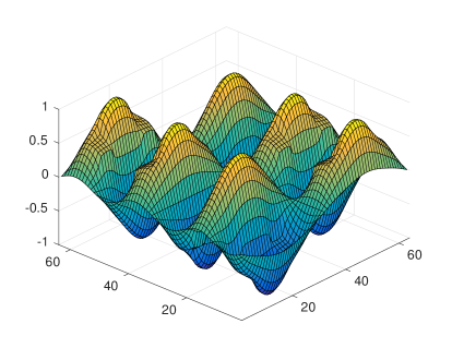
Figure 3.2: Examples of solutions $u$ for $m=255$, where $L=2$ (left) and $L=4$ (right).

Table 3.1 shows the decay of the solution error in $L_{2}$-norm estimated on a sequence of dyadic refined grids, and for different values of $L=2,4,8$. The solution is supposed to be represented on a sequence of grid in the form ${\bf u}_{p}={\bf c}_{0}+{\bf c}_{1}h_{p}^{\beta}$ up to low order term. We expect the asymptotic error behavior $O(h^{\beta})$ with $1\leq\beta\leq 2$, where in our case $\beta$ is close to $3/2$ that corresponds to decay factor $2\sqrt{2}\approx 2.8$. The latter can be expected in the case of reduced regularity in the solution caused by cusps by the multiple interior corners in the configuration of coefficient jumps. The respective convergence rate in the $H^{1}$-norm is of the order of $O(h^{\beta-1})$.

grid size $m_{p}$	$63$	$127$	$255$	$511$	$1023$
vector size $M_{d,p}$	$3969$	$16129$	$65025$	$261121$	$1046529$
$L=2$	-	$0.0051$	$0.0015$	$5.03e-04$	$1.806e-04$
$L=4$	-	$0.0057$	$0.0020$	$7.13e-04$	$2.638e-04$
$L=8$	-	-	$0.0035$	$1.40e-03$	$5.257e-04$

Table 3.1: Differences in the relative norms of solutions $\|{\bf u}_{p}-{\bf u}_{p-1}\|_{2}/\|{\bf u}_{p-1}\|_{2}$, $p=1,\ldots,5$, on dyadic refined grids computed in $L_{2}$-norm for $L=2,\;4,\;8$ and $\alpha=0.5$, $\lambda=0.1$.

Figure 3.2 illustrates examples of the solution ${\bf u}$ discretized over $m\times m$ grid with the univariate grid size $m=255$ and for $L=2$ and $L=4$.

Figure 3.3 represents differences in solutions on pair of $m\times m$ grids with $m=127,\;255$ (left) and $m=511,\;1023$ (right) for $f=sin(2\pi x)cos(6\pi y)$ and fixed $L=4$. One can observe the expected increase in the approximation error towards the interior corners in the geometry specifying the jumping coefficient function. The error decays by a factor about $10$ which agrees with the expected decay by $2.8^{2}$. For ease of comparison both solutions are interpolated onto the common grid with $m=63$.

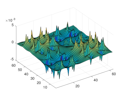
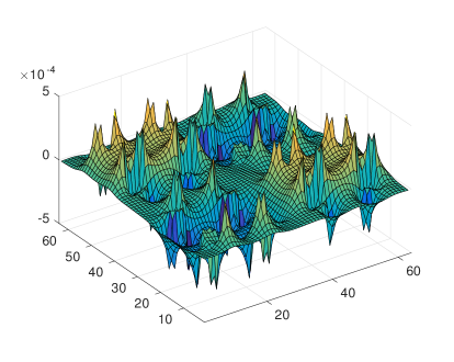
Figure 3.3: Differences in solutions on the $m\times m$ grids with $m=127,\;255$ (left) and $m=511,\;1023$ (right) for $L=4$.

3.5 Preconditioned CG iteration

Let the right-hand side in (3.3) satisfy $\langle F,1\rangle=0$, then for a fixed $m$, the equation

$$A^{(n)}{\bf u}=(\lambda A_{\Delta}+(1-\lambda)A^{(n)}_{s}){\bf u}={\bf f}$$ (3.15)

has the unique solution. We solve this equation by the preconditioned conjugate gradient (PCG) iteration (routine pcg in Matlab library) with the preconditioner

$$B=\frac{1+\lambda}{2}A_{\Delta}+\delta I=\frac{1+\lambda}{2}\Delta_{h}+\delta I,$$

where $\delta>0$ is a small regularization parameter introduced only for stability reasons (can be ignored in the theory) and $I$ is the $M_{d}\times M_{d}$ identity matrix.

It can be proven that the condition number of preconditioned matrix is uniformly bounded in $m_{1}$, $L$ and in the number of stochastic realizations $n=1,\ldots,N$. The particular estimates on the condition number in terms of a parameter $\lambda$ can be derived by introducing the average coefficient

$${a}_{0}(x)=\frac{1}{2}(a^{+}(x)+a^{-}(x)),$$

where $a^{+}(x)$ and $a^{-}(x)$ are chosen as majorants and minorants of $a^{(n)}(x)$ in (2.4), respectively. The following simple result holds.

Lemma 3.3

Given the preconditioner $B$ with $\delta=0$, then the condition number of the preconditioned matrix $B^{-1}{A}^{(n)}$ is bounded by

$$cond\{B^{-1}{A}^{(n)}\}\leq C{\lambda}^{-1}.$$

Proof. Lemma 4.1 in [15] shows that the preconditioner $A_{0}$ generated by the coefficient ${a}_{0}(x)=\frac{1}{2}(a^{+}(x)+a^{-}(x))$ allows the condition number estimate

$$cond\{{A}_{0}^{-1}{A}^{(n)}\}\leq C\max\frac{1+q}{1-q},\quad\mbox{with}\quad q:=\max(a^{+}(x)-{a}_{0}(x))/{a}_{0}(x)<1.$$

The preconditioner $B$ corresponds to the choice $a^{+}(x)=1$ and $a^{-}(x)=\lambda$, hence, we obtain ${a}_{0}(x)=\frac{1+\lambda}{2}$ and the result follows.   

The PCG solver for the system of equations (3.8) with the shifted discrete Laplacian as the preconditioner demonstrates robust convergence with the rate $q\ll 1$. In the practically interesting case $\alpha\approx 0.5$ we found that $q$ does not depend on $\lambda$. This can be explained by the fact that in this case the total overlap in all subdomains covers the large portion of the computational box $\Omega$. In all numerical examples considered so far the number of PCG iterations was smaller than $10$ for the residual stopping criteria $\delta=10^{-8}$. We use the univariate grid size $m_{1}=m_{s}$, corresponding to the choice $p=0$ in (3.1) which is fine enough to resolve geometry for larger $L$.

4 Asymptotic convergence to the stochastic average

In this section, we describe the computational scheme for calculation of the homogenized coefficient matrix for each stochastic realization.

4.1 Computational scheme for the stochastic average

For fixed stochastic realizations specifying the variable part in the $2\times 2$ coefficient matrix $\widehat{\mathbb{A}}^{(n)}(x)$, $n=1,\ldots,N$, we consider the problems

$$-\lambda\Delta\phi_{i}-(1-\lambda)\nabla\cdot\widehat{\mathbb{A}}^{(n)}(\cdot)({\bf e}_{i}+\nabla\phi_{i})=0,$$ (4.1)

for $i=1,2$. The right-hand side in equation (4.1), rewritten in the canonical form (2.8), reads as

$$f_{i}(x)=(1-\lambda)\nabla\cdot\widehat{\mathbb{A}}^{(n)}(x){\bf e}_{i}.$$

Taking into account (2.4), where the diagonal of $\widehat{\mathbb{A}}^{(n)}(x)$ is defined in terms of the scalar function $\widehat{a}^{(n)}(x)$, we arrive at

$$f_{1}(x)=(1-\lambda)\dfrac{\partial\widehat{a}^{(n)}(x)}{\partial x_{1}},\quad f_{2}(x)=(1-\lambda)\dfrac{\partial\widehat{a}^{(n)}(x)}{\partial x_{2}}.$$

Figure 4.1 illustrates an example of the calculated (reshaped) right-hand side vector in $\mathbb{R}^{m_{1}\times m_{1}}$ and the respective solution $\phi_{1}$ for $L=12$, $m_{1}=193$, and $m_{0}=16$.

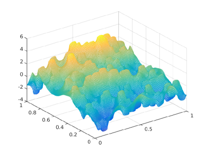
Figure 4.1: Right-hand side (left) and the solution $\phi_{1}$ (right) for $L=12$, $m_{1}=193$, $m_{0}=16$.

Fixed $L$, for the particular realization $\mathbb{A}^{(n)}$, by definition, the averaged coefficient matrix $\bar{\mathbb{A}}^{(n)}_{L}=\bar{\mathbb{A}}^{(n)}=[\bar{a}^{(n)}_{ij}]\in\mathbb{R}^{2\times 2}$, $i,j=1,2$, with the constant entries is given by

$$\bar{\mathbb{A}}^{(n)}{\bf e}_{i}=\int_{\Omega}\mathbb{A}^{(n)}(x)({\bf e}_{i}+\nabla\phi_{i})dx,$$ (4.2)

which implies the representation for matrix elements

$$\bar{a}^{(n)}_{L,ij}\equiv\bar{a}^{(n)}_{ij}=\int_{\Omega}[(\lambda I_{2\times 2}+(1-\lambda)\widehat{\mathbb{A}}^{(n)}(x))({\bf e}_{i}+\nabla\phi_{i})]_{j})dx,\quad i,j=1,2.$$

The latter leads to the entry-wise representation of the matrix $\bar{\mathbb{A}}^{(n)}=[\bar{a}^{(n)}_{ij}]$, $i,j=1,2$,

$$\bar{a}^{(n)}_{11}=\int_{\Omega}a^{(n)}(x)\Bigl{(}\dfrac{\partial\phi_{1}}{\partial x_{1}}+1\Bigr{)}dx,$$

$$\bar{a}^{(n)}_{12}=\int_{\Omega}a^{(n)}(x)\dfrac{\partial\phi_{1}}{\partial x_{2}}dx,$$

$$\bar{a}^{(n)}_{21}=\int_{\Omega}a^{(n)}(x)\dfrac{\partial\phi_{2}}{\partial x_{1}}dx,$$

$$\bar{a}^{(n)}_{22}=\int_{\Omega}a^{(n)}(x)\Bigl{(}\dfrac{\partial\phi_{2}}{\partial x_{2}}+1\Bigr{)}dx.$$ (4.3)

The representation (4.1) ensures the symmetry of the homogenized matrix $\bar{\mathbb{A}}^{(n)}$, i.e. $\bar{a}^{(n)}_{ij}=\bar{a}^{(n)}_{ji}$. Indeed, we calculate the difference between the scalar product of the first equation in (4.1) with $\phi_{2}$,

$$\langle\lambda\nabla\phi_{1}+(1-\lambda)\widehat{\mathbb{A}}^{(n)}\nabla\phi_{1},\nabla\phi_{2}\rangle-(1-\lambda)\langle\nabla\cdot\widehat{\mathbb{A}}^{(n)}(\cdot){\bf e}_{1},\phi_{2}\rangle=0,$$

and the second equation in (4.1) with $\phi_{1}$,

$$\langle\lambda\nabla\phi_{2}+(1-\lambda)\widehat{\mathbb{A}}^{(n)}\nabla\phi_{2},\nabla\phi_{1}\rangle-(1-\lambda)\langle\nabla\cdot\widehat{\mathbb{A}}^{(n)}(\cdot){\bf e}_{2},\phi_{1}\rangle=0,$$

and get the relation

$$\langle\dfrac{\partial\widehat{a}^{(n)}}{\partial x_{1}},\phi_{2}\rangle-\langle\dfrac{\partial\widehat{a}^{(n)}}{\partial x_{2}},\phi_{1}\rangle=0,$$

which then implies the desired property via integration by parts, and taking into account the relation (2.5),

$$\langle a^{(n)},\dfrac{\partial\phi_{2}}{\partial x_{1}}\rangle=\langle a^{(n)},\dfrac{\partial\phi_{1}}{\partial x_{2}}\rangle.$$

In numerical implementation, we apply the Galerkin scheme for FEM discretization of equation (4.1) its right-hand side. We use the same quadrature rule for computation of integrals in (4.1) thus preserving the symmetry in the matrix $\mathbb{A}^{(n)}$ inherited from the exact variational formulation (see argument above and Section 4.3 for the more detailed discussion).

Integrals over $\Omega$ in (4.2), (4.1) for the matrix entries $(\bar{\mathbb{A}}^{(n)})_{i,j}$, $i,j=1,2$, are calculated (approximately) by the scalar product of the $N$-vector of all-ones with the discrete representation of integrand on the grid $\Omega_{h}$, see Figure 3.1.

Tol. $\delta$	$10^{-3}$	$10^{-4}$	$10^{-5}$	$10^{-6}$	$10^{-7}$	$10^{-8}$	$10^{-9}$	$10^{-10}$	$10^{-11}$
$\|\mathbb{A}-\mathbb{A}^{T}\|$	$10^{-6}$	$3\;10^{-7}$	$10^{-7}$	$3\;10^{-9}$	$10^{-10}$	$3.6\;10^{-11}$	$10^{-11}$	$10^{-12}$	$5.7\;10^{-15}$

Table 4.1: Symmetry in the matrix $\bar{\mathbb{A}}^{(n)}_{L}$, with fixed $n$, vs. residual stopping criteria $\delta$.

To complete this section, we check numerically that the FEM discretization scheme preserves the symmetry in the matrix $\bar{\mathbb{A}}^{(n)}_{L}$ for fixed $L$ if the discrete system of equations (3.2) is solved accurately enough. Table 4.1 demonstrates that the symmetry in the matrix $\bar{\mathbb{A}}^{(n)}_{L}$ with fixed $n$ is recovered on the level of residual stopping criteria $\delta>0$ in the preconditioned iteration for solving the discrete system of equations. For this calculation we set $L=4$, $m_{0}=8$, $\alpha=0.5$ and $\lambda=0.2$.

4.2 Asymptotic of systematic error and standard deviation

The set of numerical approximations $\{\bar{\mathbb{A}}^{(n)}_{L}\}$ to the homogenized matrix $\mathbb{A}_{\mbox{\footnotesize hom}}$ is calculated by (4.2) for the sequence $\{\mathbb{A}^{(n)}_{L}(x)\}$ of $n=1,...,N$ realizations, where $N$ is large enough, and the artificial period $L$ defines the size of Representative Volume Elements (RVE). For a fixed $L$, the approximation $\bar{\mathbb{A}}^{N}_{L}$ is computed as the empirical average of the sequence $\{\bar{\mathbb{A}}^{(n)}_{L}\}_{n=1}^{N}$,

$$\bar{\mathbb{A}}^{N}_{L}=\frac{1}{N}\sum^{N}_{n=1}\bar{\mathbb{A}}^{(n)}_{L}.$$ (4.4)

By the law of large numbers we have that the empirical average converges almost surely to the ensemble average (expectation)

$$\langle\bar{\mathbb{A}}_{L}\rangle_{L}=\lim\limits_{N\to\infty}\bar{\mathbb{A}}^{N}_{L}.$$ (4.5)

Furthermore, by qualitative homogenization theory, as the artificial period $L\to\infty$, this converges to the homogenized matrix

$$\mathbb{A}_{\mbox{\footnotesize hom}}:=\lim\limits_{L\to\infty}\langle\bar{\mathbb{A}}_{L}\rangle_{L}.$$ (4.6)

In what follows, we use the entry-wise notation for $d\times d$ matrices ${\mathbb{A}}=[a_{ij}]$, $i,j=1,\ldots,d$, for example, $\langle\bar{\mathbb{A}}_{L}\rangle=[\bar{a}_{L,ij}]$ and $\bar{\mathbb{A}}_{L}^{(n)}=[\bar{a}_{L,ij}^{(n)}]$, etc.

In terms of square expectations, the convergence rate for the computable quantities can be estimated by, see [6],

$$\left\langle|\bar{\mathbb{A}}^{N}_{L}-\mathbb{A}_{\mbox{\footnotesize hom}}|^{2}\right\rangle_{L}^{1/2}\leq\frac{C_{1}}{\sqrt{N}}L^{-d/2}+C_{2}L^{-d}\log^{d}L.$$ (4.7)

We numerically study the asymptotic of both terms on the right-hand side of (4.7) separately by considering the random part of the error,

$$var^{1/2}_{L}(\bar{\mathbb{A}}_{L})=\langle\left|\mathbb{A}_{\mbox{\footnotesize hom}}-\langle\bar{\mathbb{A}}_{L}\rangle_{L}\right|^{2}\rangle_{L}^{1/2}\leq C_{1}L^{-d/2},$$ (4.8)

and the systematic error

$$\left|\mathbb{A}_{\mbox{\footnotesize hom}}-\langle\bar{\mathbb{A}}_{L}\rangle_{L}\right|\leq C_{2}L^{-d}\log^{d}L,$$ (4.9)

where $\langle\bar{\mathbb{A}}_{L}\rangle_{L}$ is calculated for large enough $N$.

4.3 Covariances of the homogenized matrix in the form of quartic tensor

Let $\langle\cdot\rangle_{L}$ be an ensemble of uniformly elliptic symmetric coefficient fields on the $d$-dimensional torus $[0,L)^{d}$. Assume that it is invariant under translation (stationary) and under the group ${\mathcal{G}}$ of all orthogonal transformations $R$ of $\mathbb{R}^{d}$ that leave the (hyper-)cube $[0,L)^{d}$ invariant (this is generated by rotations in one of the Cartesian two-dimensional planes and reflections along any Cartesian hyper-plane) in the sense of (4.22) below. In case of isotropic (i.e. scalar) coefficient fields $\mathbb{A}(x)$, (4.22) turns into

$$\mathbb{A}(R\cdot)\;\mbox{and}\;\mathbb{A}\;\mbox{have the same distribution under}\;\langle\cdot\rangle_{L},$$

which is certainly the case for the ensembles we consider numerically.

Let $X$ be a finite-dimensional space of functions on the torus $[0,L)^{d}$ of side-length $L$ with square-integrable gradients, e.g. coming from continuous, piecewise affine Finite Elements. For a given realization $\mathbb{A}(x)=\mathbb{A}^{(n)}(x)$ of the coefficient field and any direction $i=1,\cdots,d$, we consider $\phi_{i}\in X$ defined through

$$\forall\;\psi\in X\quad\int_{[0,L)^{d}}\nabla\psi\cdot\mathbb{A}({\bf e}_{i}+\nabla\phi_{i})=0,$$ (4.10)

where ${\bf e}_{i}$ denotes the unit vector in direction $i$. If $X$ contains the constant functions (as would be the case for the Finite Element space), $\phi_{i}$ has to be normalized to be unique, e.g. by imposing $\int_{[0,L)^{d}}\phi_{i}=0$, but this should be irrelevant since we are only interested in $\nabla\phi_{i}$. If $X$ is indeed a Finite Element space, and if $\{\psi_{\alpha}\}_{\mbox{nodes}\;\alpha}$ denotes the standard “Hütchen” basis then the (stiffness) matrix $A=[a_{\alpha\beta}]$ and the right hand side ${\bf f}=[f_{\alpha}]$ are given by

$$a_{\alpha\beta}=\int_{[0,L)^{d}}\nabla\psi_{\alpha}\cdot\mathbb{A}\nabla\psi_{\beta}\quad\mbox{and}\quad f_{\alpha}=-\int_{[0,L)^{d}}\nabla\psi_{\alpha}\cdot\mathbb{A}{\bf e}_{i}.$$ (4.11)

Here it is important to treat periodicity correctly: In practice, one identifies functions on $[0,L)^{d}$ with functions on $\mathbb{R}^{d}$ that are periodic in each (Cartesian) argument of period $L$, hence if the node $\alpha$ is such that one of the adjacent triangles crosses the boundary of the periodic cell $[0,L)^{d}\subset\mathbb{R}^{d}$, then there is a piece of $\phi_{\alpha}$ that appears on the other side. If a quadrature rule is used for computing the stiffness matrix, it is important that the same one is used for approximation of the right-hand side.

Let us consider the $d\times d$ matrix $\bar{\mathbb{A}}_{L}=[\bar{a}_{L,ij}]=\bar{\mathbb{A}}_{L}(\mathbb{A})$ defined through (see also (4.2))

$$\bar{a}_{L,ij}:={\bf e}_{j}\cdot\int_{[0,L)^{d}}\mathbb{A}({\bf e}_{i}+\nabla\phi_{i}),$$ (4.12)

(where again, the same quadrature rule should be used). Then we have for every realization

$$\bar{\mathbb{A}}_{L}\;\;\mbox{is symmetric, i.e.}\;\;\bar{a}_{L,ij}=\bar{a}_{L,ji}.$$ (4.13)

Let us consider the ensemble average $\langle\bar{\mathbb{A}}_{L}\rangle_{L}$, which by the law of large numbers is given by (see also (4.5))

$$\langle\bar{\mathbb{A}}_{L}\rangle_{L}=\lim_{N\uparrow\infty}\frac{1}{N}\sum_{n=1}^{N}\bar{\mathbb{A}}_{L}^{(n)},$$ (4.14)

almost surely, where $\bar{\mathbb{A}}_{L}^{(n)}$ come via (4.12) from independent realizations $\mathbb{A}=\mathbb{A}^{(n)}$ according to the distribution $\langle\cdot\rangle_{L}$. Suppose that the finite-dimensional space $X$ is invariant under reflections in the coordinate directions in the sense of (4.23) below. This imposes a more serious restriction on the Finite Element space, namely that it is based on a subdivision of the torus $[0,L)^{d}$ into axi-parallel cubes (instead of triangles) and that the function space on each cube is spanned by functions that are multi-linear in the Cartesian coordinates (as opposed to affine). If this condition is satisfied, then we have

$$\langle\bar{\mathbb{A}}_{L}\rangle_{L}\;\mbox{is isotropic, i.e.}\;\langle\bar{a}_{L,ij}\rangle_{L}=\lambda_{L}\delta_{ij}$$ (4.15)

for some $\lambda_{L}\in(0,L)$.

We are interested in the covariances of the entries of $\bar{\mathbb{A}}_{L}$, and note that by the law of large numbers

$${\rm cov}_{\langle\cdot\rangle_{L}}[\bar{a}_{L,ij},\bar{a}_{L,i^{\prime}j^{\prime}}]:=\big{\langle}(\bar{a}_{L,ij}-\langle\bar{a}_{L,ij}\rangle_{L})(\bar{a}_{L,i^{\prime}j^{\prime}}-\langle\bar{a}_{L,i^{\prime}j^{\prime}}\rangle_{L})\big{\rangle}_{L}$$

$$=\lim_{N\uparrow\infty}\frac{1}{N-1}\sum_{n=1}^{N}\big{(}\bar{a}_{L,ij}^{(n)}-\frac{1}{N}\sum_{m=1}^{N}\bar{a}_{L,ij}^{(m)}\big{)}\big{(}\bar{a}_{L,i^{\prime}j^{\prime}}^{(n)}-\frac{1}{N}\sum_{m^{\prime}=1}^{N}\bar{a}_{L,i^{\prime}j^{\prime}}^{(m^{\prime})}\big{)}.$$

More precisely, we are interested in its rescaled version

$$\bar{Q}_{L,iji^{\prime}j^{\prime}}:=L^{d}{\rm cov}_{\langle\cdot\rangle_{L}}[\bar{a}_{L,ij},\bar{a}_{L,i^{\prime}j^{\prime}}]$$

which is easier to understand as the four-linear form

$$\bar{Q}_{L}(\eta,\xi,\eta^{\prime},\xi^{\prime}):=L^{d}{\rm cov}_{\langle\cdot\rangle_{L}}[\eta\cdot\bar{\mathbb{A}}_{L}\xi,\eta^{\prime}\cdot\bar{\mathbb{A}}_{L}\xi^{\prime}].$$

We claim that it has the invariance property

$$\bar{Q}_{L}(R\eta,R\xi,R\eta^{\prime},R\xi^{\prime})=\bar{Q}_{L}(\eta,\xi,\eta^{\prime},\xi^{\prime}).$$ (4.16)

In the case of $d=2$, this implies that $\bar{Q}_{L}$ is just characterized by three different numbers:

$$\bar{Q}_{L}(e_{1},e_{1},e_{1},e_{2}) =\bar{Q}_{L}(e_{1},e_{1},e_{2},e_{1})=$$

$$\bar{Q}_{L}(e_{1},e_{2},e_{1},e_{1}) =\bar{Q}_{L}(e_{2},e_{1},e_{1},e_{1})=0,$$ (4.17)

$$\bar{Q}_{L}(e_{1},e_{2},e_{2},e_{2}) =\bar{Q}_{L}(e_{2},e_{1},e_{2},e_{2})=$$

$$\bar{Q}_{L}(e_{2},e_{2},e_{1},e_{2}) =\bar{Q}_{L}(e_{2},e_{2},e_{2},e_{1})=0,$$ (4.18)

$$\bar{Q}_{L}(e_{1},e_{2},e_{1},e_{2}) =\bar{Q}_{L}(e_{1},e_{2},e_{2},e_{1})=$$

$$\bar{Q}_{L}(e_{2},e_{1},e_{1},e_{2}) =\bar{Q}_{L}(e_{2},e_{1},e_{2},e_{1}),$$ (4.19)

$$\bar{Q}_{L}(e_{1},e_{1},e_{2},e_{2}) =\bar{Q}_{L}(e_{2},e_{2},e_{1},e_{1}),$$ (4.20)

$$\bar{Q}_{L}(e_{1},e_{1},e_{1},e_{1}) =\bar{Q}_{L}(e_{2},e_{2},e_{2},e_{2}).$$ (4.21)

Argument for (4.13). According to (4.10), definition (4.12) may be reformulated as

$$\bar{a}_{L,ij}=\int_{[0,L)^{d}}({\bf e}_{j}+\nabla\phi_{j})\cdot\mathbb{A}({\bf e}_{i}+\nabla\phi_{i}),$$

so that the symmetry of $\mathbb{A}$ yields the symmetry of $\bar{\mathbb{A}}_{L}$.

Argument for (4.15). Identifying the points on the torus with $[0,L)^{d}\subset\mathbb{R}^{d}$, let ${\mathcal{G}}$ denote the subgroup of the orthogonal group that leaves $[0,L)^{d}$ invariant. According to our assumption, for any $R\in{\mathcal{G}}$,

$$R^{t}\mathbb{A}(R\cdot)R\;\mbox{and}\;\mathbb{A}\;\mbox{have the same distribution under}\;\langle\cdot\rangle_{L},$$ (4.22)

where $R^{t}\mathbb{A}(R\cdot)R$ denotes the matrix field $[0,L)^{d}\ni x\mapsto R^{t}\mathbb{A}(Rx)R$. According to our assumption on $X$ we have

$$\psi\in X\;\Longrightarrow\;\psi(R\cdot)\in X,$$ (4.23)

where $\psi(R\cdot)$ denotes the function $[0,L)^{d}\ni x\mapsto\psi(Rx)$.

For a fixed vector $\xi\in\mathbb{R}^{d}$, we consider $\phi_{\xi}:=\xi_{i}\phi_{i}$ (Einstein’s summation convention) and note that in view of (4.10), for given realization $\mathbb{A}=\mathbb{A}^{(n)}$, the function $\phi_{\xi}=\phi_{\xi}(\mathbb{A})$ (at least up to additive constants) is characterized by

$$\forall\;\psi\in X\quad\int_{[0,L)^{d}}\nabla\psi\cdot\mathbb{A}(\xi+\nabla\phi_{\xi})=0,$$ (4.24)

We now argue that $\phi$ transforms under $R\in{\mathcal{G}}$ as follows

$$\phi_{R\xi}(\mathbb{A};Rx)=\phi_{\xi}(R^{t}\mathbb{A}(R\cdot)R;x).$$ (4.25)

Indeed, this relies on the straightforward orthogonal transformation rule

$$\int_{[0,L)^{d}}\nabla_{y}[\psi(Ry)]\cdot\mathbb{A}(y)(R\xi+\nabla\phi_{R\xi}(y))dy$$

$$\stackrel{{\scriptstyle y=Rx}}{{=}}\int_{[0,L)^{d}}\nabla\psi(x)\cdot R^{t}\mathbb{A}(Rx)R(\xi+\nabla_{x}[\phi_{R\xi}(Rx)])dx.$$

According to (4.23) and (4.24) (with $\xi$ replaced by $R\xi$) the left-hand side vanishes for all $\psi\in X$; hence by the characterization (4.24) applied to the right-hand side, we obtain (4.25).

We now argue note that from (4.25) we obtain for the gradient $\nabla\phi_{R\xi}(\mathbb{A};Rx)=\nabla\phi_{\xi}(R^{t}\mathbb{A}(R\cdot)R;x)$ and thus for the flux $q_{\xi}(\mathbb{A};x):=\mathbb{A}(\xi+\nabla\phi_{\xi}(\mathbb{A};x))$ the transformation rule

$$q_{R\xi}(\mathbb{A};Rx)=Rq_{\xi}(R^{t}\mathbb{A}(R\cdot)R;x),$$

from which we obtain by definition (4.12) that

$$\bar{\mathbb{A}}_{L}(\mathbb{A})R\xi=R\bar{\mathbb{A}}_{L}(R^{t}\mathbb{A}(R\cdot)R)\xi.$$ (4.26)

According to (4.22) this yields the following invariance property for the symmetric matrix $\langle\bar{\mathbb{A}}_{L}\rangle_{L}$

$$\langle\bar{\mathbb{A}}_{L}\rangle_{L}R\xi=R\langle\bar{\mathbb{A}}_{L}\rangle_{L}\xi.$$

Since this holds for all $\xi\in\mathbb{R}^{d}$ and all $R\in{\mathcal{G}}$, by an argument of elementary algebra, we obtain the isotropy of $\langle\bar{\mathbb{A}}_{L}\rangle_{L}$, cf (4.15).

Argument for (4.16). This follows from (4.26) in form of

$$(R\eta)\cdot\bar{\mathbb{A}}_{L}(\mathbb{A})R\xi=\eta\cdot\bar{\mathbb{A}}_{L}(R^{t}\mathbb{A}(R\cdot)R)\xi$$

and from (4.22).

Argument for (4.21)-(4.17). The four identities in (4.19) on the variances just follow from the symmetry of the underlying random variable $\bar{\mathbb{A}}_{L}$, c.f.  (4.13), in form of

$${\bf e}_{1}\cdot\bar{\mathbb{A}}_{L}{\bf e}_{2}={\bf e}_{2}\cdot\bar{\mathbb{A}}_{L}{\bf e}_{1}.$$

The identity (4.20) follows from the symmetry of the covariance in its two arguments. The vanishing of the eight entries stated in (4.17) and (4.18) follows from (4.16) applied to the reflection $R\in{\mathcal{G}}$ given by $R{\bf e}_{1}=-{\bf e}_{1}$ and $R{\bf e}_{2}={\bf e}_{2}$. The identity (4.21) follows from (4.16) applied to the reflection $R\in{\mathcal{G}}$ given by $R{\bf e}_{1}={\bf e}_{2}$ and $R{\bf e}_{2}={\bf e}_{1}$.

5 Numerical study of stochastic homogenization

In this section, we estimate numerically the mean constant coefficient in the system (2.8) depending on $L$ and other model parameters at the limit of $N\to\infty$, see [10, 8] for the respective problem setting.

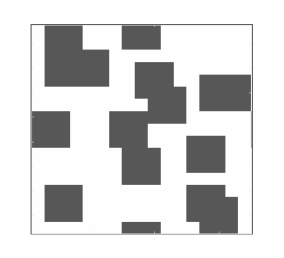
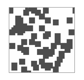
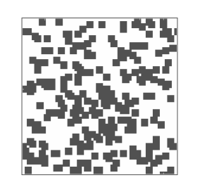
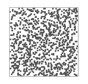
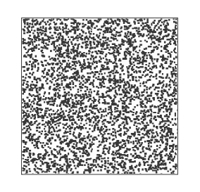
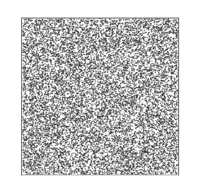
Figure 5.1: Realization examples of a stochastic process with $L^{2}$ overlapping cells for $L=4,8,16$ (top) and $L=32,64,128$ (bottom), $\alpha=1/4$.

Recall that the homogenization problem is solved in the unit square $\Omega=[0,1]^{2}$ with the grid size $m_{s}\times m_{s}$, where $m_{s}=m_{0}\,L+1$. Due to tensor-based construction of the stiffness matrix and sparse representation of matrix entities, in our numerical experiments using MATLAB, the largest number of generated homogenization cells in the domain $\Omega$ reaches the value up to $L^{2}=128^{2}$. It corresponds to the problem (vector) size $263169$ ($m_{s}=513$ with $m_{0}=4$).

Figure 5.1 illustrates examples of distributions of $L^{2}$ randomly located (overlapping) cells specifying the equation coefficient in the cases of moderate and large size of the representative volume elements (RVE) for $L=4,\,\ldots,\,128$, used in the study of asymptotic of empirical variance/average versus the size of the RVE, $L$.

$L^{2}$	$m$/$m^{2}$	matrix	RHS	PCG time
$4^{2}$	17/289	0.012	0.01	0.006
$8^{2}$	33/1089	0.06	0.045	0.137
$16^{2}$	65/4225	0.34	0.19	0.11
$32^{2}$	129/16641	3.0	0.8	0.5
$64^{2}$	257/66049	36	3.7	2.6
$128^{2}$	513/263169	561	22	13.8

Table 5.1: CPU times (sec) versus the number of inclusions (i.e., $L^{2}$) for generating the stiffness matrix, the right-hand side, and for the solution of the discretized system for the case of overlapping inclusions. Tolerance $\varepsilon=10^{-8}$.

Table 5.1 presents the CPU times for generating the stiffness matrix, the right-hand side (RHS), and for the solution of the discretized system for the case of overlapping inclusions, for tolerance $\varepsilon=10^{-8}$. Number of inclusions ($L^{2}$) varies from $16$ to $16384$. The latter is computed on a mesh of size $513\times 513$. We observe that matrix generation takes the dominating time.

5.1 Systematic error and empirical variance versus $L$

In what follows, we numerically check the theoretical convergence rate (4.7), in form of checking (4.8) and (4.9) separately.

Figure 5.2 serves to illustrate the asymptotic convergence of the systematic error see (4.9), at the limit of large $L$. Since we do not have access to the ensemble averages $\langle\bar{\mathbb{A}}_{L}\rangle_{L}$, we take empirical averages $\bar{\mathbb{A}}_{L}^{N}$ for large enough $N$, (cf. (4.6)) as a proxy. Furthermore, due to the fact that $\mathbb{A}_{\mbox{\footnotesize hom}}$ is not computable we compare the differences in $\langle\bar{a}_{L,11}\rangle_{L}$ computed on a sequence of increasing values of $L$.

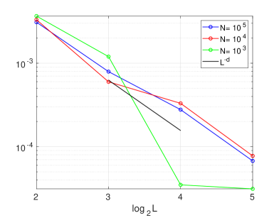
Figure 5.2: Systematic error $\langle\bar{a}_{L,11}\rangle_{L}-\langle\bar{a}_{2L,11}\rangle_{2L}$ vs. $L$, for increasing $L=2^{p}$, $p=1,\;2,\,\ldots,5$ computed for the largest number of realizations $N=10^{5}$.

Figure 5.2 shows the differences in matrix entries $\langle\bar{a}_{L,11}\rangle_{L}-\langle\bar{a}_{2L,11}\rangle_{2L}$ for increasing sizes of the RVE, i.e., for $L=2^{p}$, $p=1,\;2,\,\ldots,5$, computed with $N=10^{5}$, $N=10^{4}$ and $N=10^{3}$ stochastic realizations. It illustrates the asymptotic convergence of the systematic error, see (4.9),

$$\left|\langle\bar{\mathbb{A}}_{L}\rangle_{L}-\mathbb{A}_{\mbox{\footnotesize hom}}\right|\lesssim L^{-d}\log^{d}L$$

at the limit of large $L$. Calculations are performed with $m_{0}=4$, $\alpha=\frac{1}{4}$ and $\lambda=0.4$ and tolerance $\varepsilon=10^{-8}$. The black line corresponds to the curve $L^{-d}$, with $d=2$.

The largest size of RVE with $p=\log_{2}L=5$, presented in statistics in Figure 5.2, corresponds to the most left picture in the bottom row in Figure 5.1. In this example the jumping coefficient contains $32^{2}$ (overlapping) inclusions, and the discrete problem of size $m_{s}^{2}=129^{2}$ (i.e., vector size is $16641$) has been solved $N=10^{5}$ times for providing the representative statistics. For readers convenience, Table 5.2 presents the same data visualized in Figure 5.2.

L / N	$10^{5}$	$10^{4}$	$10^{3}$
4	0.003095	0.003316	0.003665
8	0.000792	0.000598	0.001198
16	0.000277	0.000330	-0.000034
32	0.000067	0.000077	0.000031

Table 5.2: Systematic error $\langle\bar{a}_{L,11}\rangle_{L}-\langle\bar{a}_{2L,11}\rangle_{2L}$ vs. $L$, for increasing $L=2^{p}$, $p=1,\;2,\,\ldots,5$, computed for $N=10^{5},10^{4}$ and $10^{3}$ realizations.

We now turn to the random error, i.e., the variance of $\langle\bar{\mathbb{A}}_{L}\rangle_{L}=[\bar{a}_{ij}]$. Since by symmetry considerations, $\langle\bar{a}_{11}\rangle_{L}=\langle\bar{a}_{22}\rangle_{L}$ and $\langle\bar{a}_{12}\rangle_{L}=0$, we monitor

$$\langle(\bar{a}_{L,11}-\bar{a}_{L,22})^{2}\rangle^{1/2}_{L}\quad\mbox{and}\quad\langle(\bar{a}_{L,12})^{2}\rangle^{1/2}_{L},$$

which should decay as $1/L$. Again, since we do not have access to the ensemble averages defining the standard deviation, we replace them by their empirical approximation for large enough $N$,

$$\left(\frac{1}{N}\sum\limits_{n=1}^{N}(\bar{a}_{L,12}^{(n)})^{2}\right)^{1/2}\approx\; \langle(\bar{a}_{L,12})^{2}\rangle^{1/2}_{L}\leq C_{1}L^{-d/2},$$ (5.1)

$$\left(\frac{1}{N}\sum\limits_{n=1}^{N}(\bar{a}_{L,11}-\bar{a}_{L,22})^{2}\right)^{1/2}\approx\; \langle(\bar{a}_{L,11}-\bar{a}_{L,22})^{2}\rangle^{1/2}_{L}\leq C_{1}L^{-d/2}.$$ (5.2)

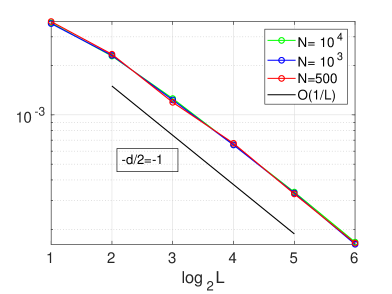
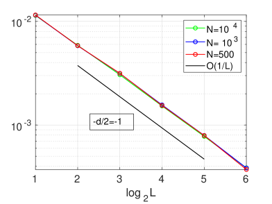
Figure 5.3: Standard deviation of $\bar{a}_{L,12}$ (left) and of $(\bar{a}_{L,11}-\bar{a}_{L,22})$ (right) versus $L$, with $L=2^{p}$, $p=1,\;2,\,\ldots,6$, for $N=500,10^{3}$ and $10^{4}$.

Figure 5.3 presents the empirical average (standard deviation) for $\bar{a}_{L,12}$ and $\bar{a}_{L,11}-\bar{a}_{L,22}$ vs. $L=2,\,4,\,\ldots,\,64$, corresponding to $N=500,10^{3}$ and $10^{4}$ realizations ($\alpha=\frac{1}{4}$, $\lambda=0.4$), confirming the estimates (5.1) and (5.2). Notice that starting from $N=500$ the values of empirical average for different number of realizations practically coincide. The results for the homogenized matrix for the largest $p=6$ presented in Figure 5.3 correspond to ensembles with $4096$ overlapping cells, and the size of the discrete problem (i.e., vector/matrix size) is $66049$. These systems of equations have been solved $10^{4}$ times. An example of realization for $p=6$ is shown in Figure 5.1 (middle bottom panel).

	$\bar{a}_{L,12}$		$\bar{a}_{L,11}-\bar{a}_{L,22}$
L / N	$10^{4}$	$500$	$10^{4}$	$500$
2	0.003643	0.003716	0.011402	0.011531
4	0.002287	0.002346	0.005875	0.005828
8	0.001258	0.001193	0.003052	0.003156
16	0.000656	0.000670	0.001527	0.001543
32	0.000337	0.000329	0.000778	0.000792
64	0.000167	0.000165	0.000386	0.000372

Table 5.3: Standard deviation of $\bar{a}_{L,12}$ (left) and $\bar{a}_{L,11}-\bar{a}_{L,22}$ (right) versus $L$, with $L=2^{p}$, $p=1,\;2,\,\ldots,6$, for $N=500$ and $N=10^{4}$.

Related to Figure 5.3, Table 5.3 presents standard deviation of $\bar{a}_{L,12}$ (left) and $\bar{a}_{L,11}-\bar{a}_{L,22}$ (right) versus $L$, with $L=2^{p}$, $p=1,\;2,\,\ldots,6$, for $N=500$ and $N=10^{4}$. We choose the following discretization and model parameters $m_{0}=4$, $\varepsilon=10^{-8}$, $\alpha=\frac{1}{4}$, and $\lambda=0.4$.

We summarize that numerical results presented in Figures 5.2 and 5.3 (see also Tables 5.2 and 5.3) confirm the asymptotic convergence rates of the systematic error (4.9) and the empirical average (5.1), (5.2) in the size $L$ of RVE.

5.2 The asymptotic of quartic tensor vs. leading order variances

In this section, we consider the convergence of the quartic tensor $\bar{Q}_{L}$, representing covariances of the matrix $\bar{\mathbb{A}}_{L}$, to its leading order variances ${Q}_{\mbox{\footnotesize hom}}$, see Section 4.3. For the large number of realizations $N$, the computable approximation, $\bar{Q}_{L}^{N}\in\mathbb{R}^{2\times 2\times 2\times 2}$, to the scaled quartic tensor is defined by

$$\bar{Q}_{L}^{N}=\frac{L^{d}}{N-1}\sum_{n=1}^{N}(\bar{\mathbb{A}}^{(n)}_{L}-\frac{1}{N}\sum_{n^{\prime}=1}^{N}\bar{\mathbb{A}}^{(n^{\prime})}_{L})^{\otimes 2},$$ (5.3)

so that by the central limit theorem

$$\bar{Q}_{L}:=\lim\limits_{N\to\infty}\bar{Q}_{L}^{N}.$$

The equivalent matrix representation of $\bar{Q}_{L}^{N}$ is obtained by setting the operation $\otimes 2$ in (5.3) as the Kronecker product of matrices (see Definition 3.1), further denoted by

$$\bar{{Q}}^{N}_{L}=[\bar{q}_{L,ij}]\in\mathbb{R}^{4\times 4},\quad i,j=1,\ldots,4.$$

In our numerical tests we shall check the asymptotic behavior

$$\left\langle\left|\frac{L^{d}}{N-1}\sum_{n=1}^{N}(\bar{\mathbb{A}}^{(n)}_{L}-\frac{1}{N}\sum_{n^{\prime}=1}^{N}\bar{\mathbb{A}}^{(n^{\prime})}_{L})^{\otimes 2}-{Q}_{\mbox{\footnotesize hom}}\right|^{2}\right\rangle_{L}\lesssim L^{-d}\ln^{d}L,$$

which can be expected at the limit of large size $L$ of the RVE, see [6, 4].

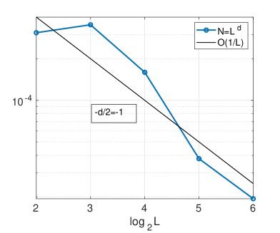
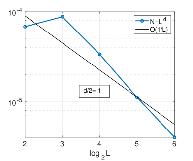
Figure 5.4: $\bar{q}_{L,11}-\bar{q}_{2L,11}$ (left) and $\bar{q}_{L,14}-\bar{q}_{2L,14}$ (right) versus $L=2^{p}$, $p=1,\ldots,6$, $N=L^{d}$.

It is worth to note that the quartic tensor $\bar{Q}_{L}$ can be calculated at no further cost than the effective homogenized matrix $\bar{\mathbb{A}}_{L}$.

Figure 5.4 shows the diagonal elements, $\bar{q}_{L,11}-\bar{q}_{2L,11}$ and $\bar{q}_{L,14}-\bar{q}_{2L,14}$, in quartic tensor $\bar{Q}_{L}^{N}$ versus increasing size of RVE $L=2^{p}$, $p=1,\ldots,6$, (see (5.3)), for $N=L^{d}$. Figure 5.4 confirms convergence rate of $\bar{q}_{L,11}-\bar{q}_{2L,11}$ in RVE $L$ as $O(L^{d/2}$.

6 Conclusions

We present the numerical scheme for discretization and solution of 2D elliptic equations with strongly varying piecewise constant coefficients arising in stochastic homogenization of multiscale composite materials. The resulting large linear system of equations is solved by the preconditioned CG iteration with the convergence rate that is independent of the grid size and of the variation in jumping coefficients. For a fixed size of the representative volume element, our approach allows to avoid the generation of the new FEM space in each stochastic realization. For every realization, fast assembling of the FEM stiffness matrix is performed by agglomerating the Kronecker tensor products of 1D FEM discretization matrices. The resultant stiffness matrix is maintained in a sparse matrix format.

Our numerical scheme allows to investigate the asymptotic convergence rate of significant quantities of stochastic homogenization process in the course of a large number of realizations (of the order of $N=10^{5}$) and for large sizes of the representative volume elements up to $L=128$, corresponding to the number of inclusions $16384$ and matrix size $513^{2}\times 513^{2}$. Note that for every realization a new matrix generation and solution of the respective linear system is performed.

Our numerical experiments study the asymptotic convergence rate of systematic error and standard deviation in the size of RVE, rigorously established in [6]. In particular, we confirm in various numerical tests the theoretical asymptotic estimates, see Section 4.2, concerning the convergence rate $O(1/L)$ for the empirical variance at the limit of large $L$, but with a moderate number of stochastic realizations $N$, and the asymptotic $CL^{-2}\ln^{2}L$ in the case of large $N$.

The asymptotic behavior of covariances of the homogenized matrix in the form of quartic tensor are studied numerically. In particular, we consider the asymptotic of the quartic tensor versus the leading order variances, computed for the large number of stochastic realizations up to $N=10^{4}$. In this way, the asymptotic $O(L^{-d}\ln^{d}L)$, for $d=2$, is confirmed on a sequence of increasing sizes of the RVE, up to $L=64$.

The stochastic characteristics of the system are analyzed for a range of intrinsic model parameters like the number of realizations, the size of periodic representative volume element, the jump-ratio in the stochastic equation coefficients (contrast) and various grid discretization parameters. The presented numerical scheme allows to perform large scale simulations using MATLAB on a moderate computer cluster. The tensor-based numerical techniques to matrix generation presented in this paper can be extended to 3D and higher dimensional problems.

7 Appendix: spectral density of a stochastic operator

Spectral properties of the randomly generated family of elliptic operators are important in many applications, in particular, in stochastic homogenization of time dependent PDEs. In what follows, we analyze numerically the average behavior of the so-called density of spectrum (DOS) for the family of stochastically generated 2D elliptic operators $\{A_{n}\}$ for the large sequence of stochastic realizations $n=1,\ldots,N$. The DOS provides the important spectral characteristics of the stochastic differential operator which accumulate the significant information on the static and dynamical characteristics of the complex physical or molecular system. Here we numerically demonstrate the convergence of DOS to the sample average function at the limit of large number of stochastic realizations with fixed $L$. Our second goal is the numerical study of the DOS depending on the increasing number $L$.

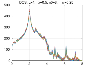
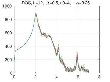
Figure 7.1: Density of states for a number of stochastic processes $N=1,\;2,\ldots,\;20$ with $L=4$ (left) and $L=12$ (right) for $\lambda=0.5$, $n_{0}=8$ and $\alpha=0.25$.

We use the simple definition of DOS for symmetric matrices, see [18, 2],

$$\phi(t)=\frac{1}{m}\sum\limits_{j=1}^{m}\delta(t-\lambda_{j}),\quad t,\lambda_{j}\in[0,a],$$ (7.1)

where $\delta$ is the Dirac function and the $\lambda_{j}$’s are the eigenvalues of $A=A^{T}\in\mathbb{R}^{m\times m}$,

$$A{\bf u}_{j}=\lambda_{j}{\bf u}_{j},\quad j=1,\ldots,m,$$

assumed to be labeled non-decreasingly.

In the presented analysis we employ the commonly used class [18] of blurring approximations to the spectral density $\phi(t)$ by using regularization via a Gaussian function with width parameter $\eta>0$,

$$\delta(t)\rightsquigarrow g_{\eta}(t)=\frac{1}{\sqrt{2\pi}\eta}\exp{\left(-\frac{t^{2}}{2\eta^{2}}\right)},$$

where the choice of small regularization parameter $\eta$ depends on the particular problem setting. The DOS in (7.1) will be approximated by Gaussian broadening,

$$\phi(t)\mapsto\phi_{\eta}(t):=\frac{1}{m}\sum\limits_{j=1}^{m}g_{\eta}(t-\lambda_{j}),\quad t\in[\lambda_{min},\lambda_{max}].$$ (7.2)

Figure 7.1 represents DOS for a sequence of $N=1,\;2,\ldots,\;20,$ stochastic realizations with $L=4,8$ from left to right, corresponding to the fixed model parameters $\lambda=0.5$, $\alpha=0.25$ and $m_{0}=8$. This figure demonstrates the clustering of DOS around the sample average on a sequence of $N$ realizations. This can be compared with DOS corresponding to the homogenized coefficient. The numerical experiments show that the spectrum of the stochastic operator strongly depends on the parameter $\alpha$ of the stochastic process. Moreover, we come to the following practically important observation.

Remark 7.1

Figure 7.1 indicates that the DOS calculated with fixed model parameters, but for different values of $L$ have practically identical shapes in the case of periodic boundary conditions. This stochastic property is the reminiscence of the corresponding feature for the deterministic lattice structured systems in the periodic super-cell.

Finally, we notice that the specific feature of the homogenized DOS is that the sample average differs substantially from DOS for the operator with the homogenized coefficient.

Acknowledgements. The authors would like to thank Julian Fischer (IST Austria, Wien) and Ronald Kriemann (MPI MiS, Leipzig) for useful discussions concerning the problem setting.

References

- [1] A. Anantharaman, R. Costaouec, C. Le Bris, F. Legoll and F. Thomines. Introduction to numerical stochastic homogenization and the related computational challenges: some recent developments. In Lecture Notes Series, Institute for Mathematical Sciences, Vol. 22, eds. Weizhu Bao and Qiang Du (National University of Singapore), 2011, pp 197–272.
- [2] P. Benner, V. Khoromskaia, B. N. Khoromskij and C. Yang. Computing the density of states for optical spectra of molecules by low-rank and QTT tensor approximation. J. Comput. Phys., 382, 2019, 221-239.
- [3] Eric Cances, Virginie Ehrlacher, Frederic Legoll, Benjamin Stamm, Shuyang Xiang. An embedded corrector problem for homogenization. Part II: Algorithms and discretization. arXiv: http://arxiv.org/abs/1810.09885v1, 2018.
- [4] Mitia Duerinckx, Antoine Gloria and Felix Otto: The structure of fluctations in stochastic homogenization. ArXiv: 1602.01717v3, 2017.
- [5] Julian Fischer. The choice of representative volumes in the approximation of the effective properties of random materials. E-preprint, arXiv:1807.00834, 2018.
- [6] Antoine Gloria, Stefan Neukamm and Felix Otto. Quantification of ergodicity in stochastic homogenization: optimal bounds via spectral gap on Glauber dynamics. In: Inventiones mathematicae, 199 (2015) 2, p. 455-515; MIS-Preprint: 91/2013, DOI: 10.1007/s00222-014-0518-z.
- [7] Antoine Gloria and Felix Otto. An optimal variance estimate in stochastic homogenization of discrete elliptic equations. Ann. Probab., 39 (3) (2011), 779-856.
- [8] Antoine Gloria and Felix Otto. The corrector in stochastic homogenization: near-optimal rates with optimal stochastic integrability. ARXIV: http://arxiv.org/abs/1510.08290, 2016.
- [9] Antoine Gloria and Felix Otto. Quantitative estimates on the periodic approximation of the corrector in stochastic homogenization. ESAIM: Proceedings and Surveys, 48 (2015), p. 80-97.
- [10] Antoine Gloria and Felix Otto: An optimal error estimate in stochastic homogenization of discrete elliptic equations. In: The annals of applied probability, 22 (2012) 1, p. 1-28. E-preprint, arXiv: http://de.arxiv.org/abs/1203.0908.
- [11] T. Kanit, S. Forest, I. Galliet, V. Mounoury and D. Jeulin. Determination of the size of the representative volume element for random composites: statistical and numerical approach. Int. J. of Solids and Structures, 40, 2003, 3647-3679.
- [12] V. Khoromskaia, B. N. Khoromskij and F. Otto. A Numerical Primer in 2D Stochastic Homogenization: CLT scaling in the Representative Volume Element. Preprint 47/2017, Max-Planck Institute for Mathematics in the Sciences, Leipzig, 2017.
- [13] B.N. Khoromskij and G. Wittum. Numerical Solution of Elliptic Differential Equations by Reduction to the Interface. Research monograph, LNCSE, No. 36, Springer-Verlag 2004.
- [14] Boris N. Khoromskij. Tensor Numerical Methods in Scientific Computing. Research monograph, De Gruyter Verlag, Berlin, 2018.
- [15] B.N. Khoromskij and S. Repin. A fast iteration method for solving elliptic problems with quasi-periodic coefficients. Russ. J. Numer. Anal. Math. Modelling 2015; 30 (6):329-344. E-preprint, arXiv:1510.00284, 2015.
- [16] B. N. Khoromskij and Ch. Schwab. Tensor-structured Galerkin approximation of parametric and stochastic elliptic PDEs. SIAM J. Sci. Comput. 33 (1), 364-385, 2011.
- [17] C. Le Bris, F. Legoll. Examples of computational approaches for elliptic, possibly multiscale PDEs with random inputs, J Comput. Phys. 328 (2017) 455–473.
- [18] L. Lin, Y. Saad, and C. Yang. Approximating spectral densities of large matrices. SIAM Review, 58(1): 34–65, 2016.