Phase space classification of an Ising Cellular Automaton: the Q2R model

Abstract

An exact characterization of the different dynamical behavior that exhibit the space phase of a reversible and conservative cellular automaton, the so called Q2R model, is shown in this paper. Q2R is a cellular automaton which is a dynamical variation of the Ising model in statistical physics and whose space of configurations grows exponentially with the system size. As a consequence of the intrinsic reversibility of the model, the phase space is composed only by configurations that belong to a fixed point or a limit cycle. In this work we classify them in four types accordingly to well differentiated topological characteristics. Three of them –which we call of type S-I, S-II and S-III– share a symmetry property, while the fourth, which we call of type AS, does not. Specifically, we prove that any configuration of Q2R belongs to one of the four previous limit cycles. Moreover, at a combinatorial level, we are able to determine the number of limit cycles for some small periods which are almost always present in the Q2R. Finally, we provide a general overview of the resulting decomposition of the arbitrary size Q2R phase space, in addition, we realize an exhaustive study of a small Ising system ($4\times 4$) which is fully analyzed under this new framework.

1 Introduction

A central problem in statistical physics concerns the manifestation of irreversibility whenever the system is governed by a large number of elements, or more precisely the number of degrees of freedom. Despite the reversible character of the equation of motions in mechanics, the nature does not allow to observe a reversible behavior of a macroscopical system. After Boltzmann theory and the subsequent Loschmidt and Zermelo’s considerations this central question has been in the core of debates in basic physics since the end of the 19th century. In particular, Zermelo argued that the Boltzmann H-theorem is in contradiction with Poincaré’s recurrence theorem, however, as Boltzmann replied, the hypothetical recurrence time would be huge in comparison with all practical times in the usual thermodynamics.

To model the recurrence time paradox, Paul and Tatiana Ehrenfest elaborated a particle exchange model [1, 2], the so-called the “dog-flea” model. This combinatorial model appears as an illustration of the irreversible exchange of heat between two distinct reservoirs at different temperatures. Ehrenfest model consists of $N$ particles that can be distributed in the left or right side of a container, in such a way that $N/2+n$ balls are initially at the left container and $N/2-n$ in the right one. As shown by M. Kac [3], the Ehrenfest model may be mapped into a random walk. Moreover, if initially the system is filling mostly one container side $n\approx N/2$, then the average recurrence time is exponentially long, $\sim 2^{N}$. On the other hand, if initially the system is almost equally distributed $n\approx 0$, then, the waiting time scales as a diffusion process $\sqrt{N}$. Therefore, as one increases the total number of degrees of freedom $N$, there are some initial conditions with exponentially long recurrence times. The interest of the extremely simplified Ehrenfest model is that captures the essence of an exponentially long recurrence time showing that some initial configuration require exponentially long time to be back to the same state again.

Generically, irreversibility arises as a consequence of systems that possess a large number of degrees of freedom. Moreover, even in moderate system size, say $N=64$ for the Ehrenfest’s model, the recurrence time becomes of the order of $2^{64}$, i.e., essentially infinity. Therefore, although irreversibility appears to be a consequence of thermodynamic limit, $N\to\infty$, in practice even in moderate system size a thermodynamic statistical description appears to be the adequate one [4].

In a recent article [5], two of us, developed a master equation approach to a reversible and conservative cellular automaton model: the Q2R model. Introduced in the 80 by Vichniac [6], Q2R is a dynamical variation of the Ising model for ferromagnetism that possesses quite a rich and complex dynamics. Remarkably, the evolution of Q2R preserves an Ising-like energy [7], appealing the analogy with the continuous dynamics of Hamiltonian systems. Because the Q2R model is a reversible cellular automaton its phase space is finite and there are neither attractive nor repulsive attractors, all attractors must be fixed points or limit cycles.

Q2R is a two variable automaton, i.e., a state is defined through $(x^{t},y^{t})$ in which each component $x^{t}$ and $y^{t}$ belong to a graph which is defined via a lattice and a neighbor (see Section 2). Although it can be defined in any kind of lattice, we restrict ourselves to the particular case of a square grid with a von-Neuman four nearest neighbors. The size of the lattice will be $N=L\times L$, thus the phase space is the set of the $2^{2N}$ vertices of a $2N$-dimensional hypercube. However, as we show in this paper, the phase space is partitioned in a large number of subspaces composed by periodic orbits or fixed points. A given initial condition belongs to one of this limit cycles or is a fixed point.

It has been reported numerically, that the phase space is composed of a huge number of limit cycles with probable exponentially long periods [8]. For small Ising systems, e.g., for a $2\times 2$ square lattice, there are $2^{8}=256$ states and the longest orbit is of period 4. In the case, of a $4\times 4$, the phase space has $2^{32}\approx 4.3\times 10^{9}$ elements, being $T=1080$ the longest limit cycle. More important, this case can be scrutinized exactly, and we are able to conjecture that the number of states of a given period is exponentially large with the number of sites $N$.

In Ref. [5], following the Nicolis and Nicolis coarse-graining approach [9], we have applied it to the time series of the total magnetization, leading to a master equation that governs the macroscopic irreversible dynamics of the Q2R automata. The methodology works out for various lattice sizes. Notably, in the case of small systems, we show that the master equation leads to a tractable probability transfer matrix of moderate size, which provides a master equation for a coarse-grained probability distribution. The success of a consistent thermodynamic description is based on the existence of rich nature of the phase space. Similarly, Lindgren and Olbrich [10] have recently considered the equilibrium properties of the Q2R model but with a different approach. Furthermore, for a large system size it has been established that the evolution presents an irreversible behavior towards an equilibrium ruled by a micro-canonical ensemble [11, 12]. Moreover, in Ref. [12], it has been shown numerically that for a set of random initial conditions with different energies one recovers statistically the Ising phase transition ruled by the Onsager and Yang exact solutions [15, 16].

The aim of the present article, is to study and classify the different possible attractors (fixed points and limit cycles) of the phase space of the Q2R cellular automaton in a square lattice of arbitrary size. The starting point is the reversibility property of the Q2R model and essentially all results of the current paper follow after the Lemma 3.16 (on Reversibility).

Our main results are the following:

1. A fully classification of all attractors in four types of limit cycles consisting of symmetric and asymmetric ones (Theorem 4.28). More precisely this characterization is according to the specific topological features of the cycle. These limit cycles may be symmetric limit cycle of type S-I, S-II and S-III (See Sec. 4.4) and asymmetric limit cycle (AS).

2. The fixed points are of type S-I, moreover with the aid of splitting the lattice in two sub lattices we are able to show that the total number of fixed points is $\beta^{2}=4k^{2}$ , with $k\in\mathbb{N}$ (Theorems 4.18 and 4.46).

3. The characterization and existence of $\beta^{2}(\beta^{2}-1)$ period-two limit cycles. (Theorems 4.22 and 4.46).

4. The characterization and existence of period-three limit cycles (Theorem 4.24 and Proposition 4.41).

The paper is organized as follows: In Section 2, we define the Q2R model and its main properties. In Section 3, we establish the formal definitions scheme, and we state the fundamental Lemma on reversibility (Lemma 3.16) which is the key property after it all results in the paper follows. In Section 4, we prove the main results listed above. Next, in Section 5, we present a general overview of the resulting decomposition of the phase space of Q2R. In Section 6 we conclude and discuss on further results and conjectures. Finally, in the Appendix 7 we provide an exhaustive study of a small Ising system ($4\times 4$) which is fully analyzed under this new framework with some specific examples of limit cycles.

2 The model

2.1 Context and definitions

The Q2R model, introduced by Vichniac [6], is defined in a regular two dimensional toroidal lattice with even rank $L\times L$, being $N=L^{2}$ the total number of nodes which have associated an index ${\bm{k}}\in\{1,\dots,N\}$, as well as a relative position in the lattice specified by two indices $k_{1}\in\{1,\dots,L\}$ and $k_{2}\in\{1,\dots,L\}$ (the respective row and column indices). Further, a node $\bm{k}$ is characterized by two possible values $x_{\bm{k}}=\pm 1$, conforming with the following two-step rule:

$$x^{t+1}_{\bm{k}}=x^{t-1}_{\bm{k}}\,H\left(\sum_{{\bm{i}}\in V_{\bm{k}}}x^{t}_{\bm{i}}\right),$$

where $V_{\bm{k}}$ denotes the von Neuman neighborhood of the four closest neighbors with periodic boundary conditions. The function $H$ is such a that $H(s=0)=-1$ and $H(s)=+1$ in all other cases.

The above two-step rule may be naturally re-written as a one step rule with the aid of a second dynamical variable [7]:

$$y^{t+1}_{\bm{k}} = x^{t}_{\bm{k}}$$

$$x^{t+1}_{\bm{k}} = y^{t}_{\bm{k}}\,H\left(\sum_{i\in V_{\bm{k}}}x^{t}_{\bm{i}}\right).$$ (2.1)

Thus, the state $x$ belongs to the discrete set $\Omega=\{-1,1\}^{N}$ (of size $2^{N}$) and the set of configurations, denoted by $\Omega^{2}$, it is composed by couples of states in $\Omega^{2}=\Omega\times\Omega=\left\{(x,y)/x\in\Omega\wedge y\in\Omega\right\}$ (of size $2^{2N}$).

Definition 2.1.

We denote the symbol $\odot$ by the Hadamard product, which is the multiplication component to component of the state $x\in\Omega$ and $y\in\Omega$. Hence, $x\odot y\in\Omega$ represents that each component is defined by: $[x\odot y]_{ij}\equiv x_{ij}y_{ij}$. This product is commutative, associative, and it possesses a neutral element, that we denote by $\mathbb{1}$ and corresponds to the state of $\Omega$ composed only by 1s. Moreover, we also define $-\mathbb{1}\in\Omega$ by the states composed only by -1s. Given $x\in\Omega$, we will write $-x$ to refer to $-x=[-\mathbb{1}]\odot x$.

Definition 2.2.

Let be the function $\phi:\Omega\to\Omega$ such that, if $x\in\Omega$ then, the $\bm{k}$-th component of $[\phi(x)]_{\bm{k}}=-1$ if the sum of all von Neuman neighbors of the $\bm{k}$-th components is null, namely $\sum_{{\bm{i}}\in V_{\bm{k}}}x_{\bm{i}}=0$. Notice that the neighborhood, $V_{\bm{k}}$, includes the periodic boundary condition of the lattice. Otherwise, $[\phi(x)]_{\bm{k}}=+1$. Therefore, the function $\phi(x)$ is a state in $\Omega$ that has a -1 in the sites that $x$ has a null neighborhood.

Example.

Consider the state $x\in\Omega$ below. The node (3,2) has null neighborhood (its neighbors are marked by boxes), while the neighborhood of the node located at (1,4) is not null (its neighbors are marked by double boxes accordingly, to the toroidal lattice). So, the state $\phi(x)$ will have a -1 value at position (3,2) and a 1 value at position (1,4) that are also marked, with a box and a double box, respectively, in $\phi(x)$. In a similar way, all other values of $\phi(x)$ are obtained.

$$x=\left[\begin{array}[]{cccc}\doublebox{1}&1&\doublebox{1}&1\\ 1&\framebox{-1}&1&\doublebox{1}\\ \framebox{1}&1&\framebox{-1}&1\\ 1&\framebox{1}&1&\doublebox{1}\\ \end{array}\right]\mapsto\phi(x)=\left[\begin{array}[]{cccc}1&1&1&\doublebox{1}\\ 1&1&-1&1\\ 1&\framebox{-1}&1&1\\ 1&1&1&1\\ \end{array}\right].$$ (2.2)

Definition 2.3.

The state $x$ does not have any null-neighborhood iff $\phi(x)=\mathbb{1}$. Notice that $\phi(\mathbb{1})=\phi(-\mathbb{1})=\mathbb{1}$.

2.2 The Q2R rule.

Given $(x^{t},y^{t})\in\Omega^{2}$ at time $t$, and according with the previous definitions we re-write the Q2R model (2.1) as the following two step deterministic rule:

$$y^{t+1} = x^{t}$$

$$x^{t+1} = y^{t}\odot\phi\left(x^{t}\right).$$ (2.3)

The evolution is dictated by the rule (2.2) and is complemented with an initial configuration $(x^{0},y^{0})\in\Omega^{2}$. For instance, let us consider $x^{0}=y^{0}=x$, the example given in (2.2). The evolution of the initial configuration $(x^{0},y^{0})$ are obtained as follows:

$\left(\underbrace{\left[\begin{array}[]{cccc}1&1&1&1\\ 1&-1&1&1\\ 1&1&-1&1\\ 1&1&1&1\end{array}\right]}_{x^{0}}\right.$	,	$\left.\underbrace{\left[\begin{array}[]{cccc}1&1&1&1\\ 1&-1&1&1\\ 1&1&-1&1\\ 1&1&1&1\end{array}\right]}_{y^{0}}\right)$
$\left(\underbrace{\left[\begin{array}[]{cccc}1&1&1&1\\ 1&-1&-1&1\\ 1&-1&-1&1\\ 1&1&1&1\end{array}\right]}_{x^{1}=y^{0}\odot\phi(x^{0})}\right.$	,	$\left.\underbrace{\left[\begin{array}[]{cccc}1&1&1&1\\ 1&-1&1&1\\ 1&1&-1&1\\ 1&1&1&1\end{array}\right]}_{y^{1}=x^{0}}\right)$
⋮		⋮

that we schematize with the following abbreviated notation:

$$(x^{0},y^{0})\to(x^{1},y^{1})\to\cdots\,.$$

Remark 2.4.

In general, we will write $(x^{t},y^{t})\to(x^{t+1},y^{t+1})$ for the one-step evolution from $(x^{t},y^{t})$ to $(x^{t+1},y^{t+1})=\left(y^{t}\odot\phi\left(x^{t}\right),x^{t}\right)$, according to rule (2.2).

Definition 2.5.

The Phase Space of the Q2R model it is composed by the set of configurations $\Omega^{2}$ and its one-step evolutions. Because is finite, the phase space has two types of attractors: limit cycles or fixed points. A limit cycle $\mathcal{C}$ of period $T\in\mathbb{N}$ is a sequence dictated by the evolution $(x^{0},y^{0})\to(x^{1},y^{1})\to\cdots\to(x^{T-1},y^{T-1})\to(x^{T},y^{T})$ such that all configurations $(x^{t},y^{t})$ are different, except $(x^{0},y^{0})=(x^{T},y^{T})$. We will write $(x,y)\in\mathcal{C}$ if $(x,y)$ is a configuration that is in $\mathcal{C}$ and, more general, the notation $[(x^{t},y^{t})\to(x^{t+1},y^{t+1})\to\cdots\to(x^{t+\tau},y^{t+\tau})]\in\mathcal{C}$ will be used to refer to the subsequence of $\mathcal{C}$ that goes from $(x^{t},y^{t})$ to $(x^{t+\tau},y^{t+\tau})$, $\tau\leq T$. A fixed point is a limit cycle of period $T=1$, i.e., is a configuration $(x,y)\in\Omega^{2}$ such that $(x,y)\to(x,y)$.

2.3 Main properties

2.3.1 Reversibility

Observe that $\phi\left(x^{t}\right)\odot\phi\left(x^{t}\right)=\mathbb{1},\,\forall x^{t}\in\Omega$. Then Q2R rule may be inverted getting the backward evolution of the system but for the couple $(y^{t},x^{t})$, that reads:

$$\left\{\begin{array}[]{l}x^{t-1}=y^{t}\\ y^{t-1}=x^{t}\odot\phi\left(y^{t}\right),\end{array}\right.$$ (2.6)

which is exactly the same rule (2.2), displaying the remarkable property of reversibility. This property will be highlighted in the “Reversibility Lemma” (Lemma 3.16).

2.3.2 Configurations of the phase space

Since the Q2R rule is reversible and the phase space is finite, each configuration has two possibilities; to be a fixed point or to belong in a limit cycle.

2.3.3 Dynamical Invariants: The energy.

Definition 2.6.

Let be the energy function

$$E[\left(x^{t},y^{t}\right)]=-\frac{1}{2}\sum_{\left<{\bm{i}},{\bm{k}}\right>}x^{t}_{\bm{i}}y^{t}_{\bm{k}},$$ (2.7)

where the symbol $\left<\cdots\right>$ stands for sum over the four near neighbors. The energy (2.7) is bounded by $-2N\leq E\leq 2N$.

Remark 2.7.

As shown by Pomeau [7], the energy function (2.7) is conserved, under the dynamics defined by the Q2R rule (2.2). That is $E[\left(x^{t},y^{t}\right)]=E[\left(x^{0},y^{0}\right)],\,\forall t\in\mathbb{N}$.

Remark 2.8.

Other dynamical invariants are known in the literature [13].

2.3.4 The phase space and the qualitative dynamics

The phase space of all configurations is defined through all possible values of the $2N$ dimensional state $(x,y)\in\Omega^{2}$. The resulting phase space is composed by the $2^{2N}$ vertices of a hypercube in dimension $2N$. This phase space is partitioned in different sub-spaces accordingly to its energy, $E$, and accordingly with its dynamical characteristic such that the period, and other unknown parameters.

For instance, the constant energy subspace shares in principle many limit cycles of different periods, as well as, many different fixed points. An arbitrary initial condition of energy $E$, falls into one of these limit cycles, and it runs until a time $T$, which could be exponentially long, and displaying a complex behavior (not chaotic stricto-sensu, see for instance [14]). More important, the probability that an initial condition belongs to an exponentially long period limit cycle and it exhibits a complex behavior is finite [8]. Moreover, Q2R manifests sensitivity to initial conditions, that is, if one starts with two distinct, but close, initial conditions, then, they will evolve into very different limit cycles as time evolves [12]. In some sense, any initial state explores vastly the phase space justifying the grounds of statistical physics, as we shown in the Remark 3.10 and the main Theorem 4.28 on the limit cycle general classification.

3 Preliminary Results

The core of this work aims to propose a new framework to study the dynamic of the Q2R model. It is based in particular properties of its configurations that allow to partition $\Omega^{2}$ in order to characterize the full spectrum of fixed points and limit cycles, as well as delving into topological and combinatorial aspects. We begin by establishing the basic concepts that will be used along the text and the first results, necessary to understand the main results (Section 4).

3.1 Partitions of $\Omega^{2}$.

Observe that, given the states $x,y\in\Omega$, there are two possibilities: $[x=y]$ or $[x\neq y]$. Therefore a first partition of $\Omega^{2}$ arises as follows:

Definition 3.9.

We denote by $\Omega^{2}_{xx}$ the set of configurations with equal states, i.e.,

$$\Omega^{2}_{xx}=\left\{(x,y)\in\Omega^{2}/x=y\right\},$$

whose size is $|\Omega^{2}_{xx}|=2^{N}$. Similarly, the set of configurations with different states will be denoted by $\Omega^{2}_{xy}$ and corresponds to the complement set of $\Omega^{2}_{xx}$ in $\Omega^{2}$, i.e.,

$$\Omega^{2}_{xy}=\Omega^{2}-\Omega^{2}_{xx}=\left\{(x,y)\in\Omega^{2}/x\neq y\right\}$$

whose size is $|\Omega^{2}_{xy}|=2^{N}(2^{N}-1)$. Note that: $\Omega^{2}=\Omega^{2}_{xx}\cup\Omega^{2}_{xy}.$

Remark 3.10.

We underline that $|\Omega^{2}_{xx}|<|\Omega^{2}_{xy}|$. Further, the probability to have a configuration in $\Omega^{2}_{xx}$ is $p_{xx}=|\Omega^{2}_{xx}|/|\Omega^{2}|=2^{-N}$, while the probability to have a configuration in $\Omega^{2}_{xy}$, is $p_{xy}=|\Omega^{2}_{xy}|/|\Omega^{2}|=1-2^{-N}$. Hence, in practice, $p_{xx}\ll p_{xy}$. Moreover $p_{xy}\to 1$ in the thermodynamic limit ($N\to\infty$).

A second partition of $\Omega^{2}$ will allow us to know in detail the topology of the limit cycles: here, the sets $\Omega^{2}_{xx}$ and $\Omega^{2}_{xy}$ are also partitioned regarding the two possibilities of $\phi(x)$ in a configuration $(x,y)$, that is $[\phi(x)=\mathbb{1}]$ or $[\phi(x)\neq\mathbb{1}]$, regardless the value of $\phi(y)$, as in the following definition:

Definition 3.11.

Let be the following sets:

$$A = \left\{(x,y)\in\Omega_{xx}^{2}/\phi(x)=\mathbb{1}\right\}$$

$$B = \left\{(x,y)\in\Omega_{xy}^{2}/\phi(x)=\mathbb{1}\right\}$$

$$C = \left\{(x,y)\in\Omega_{xx}^{2}/\phi(x)\neq\mathbb{1}\right\}$$

$$D = \left\{(x,y)\in\Omega_{xy}^{2}/\phi(x)\neq\mathbb{1}\right\}.$$

We say that $(x,y)\in\Omega^{2}$ is a configuration of type $A$, $B$, $C$ or $D$, if $(x,y)$ belongs to one of the sets $A$, $B$, $C$ or $D$, respectively. Later on, we refer to a evolution of type $U\to V$ to the one step evolution of a configuration $(x,y)\in U$ up to $(w,x)\in V$ with $U,V\in\{A,B,C,D\}$. In such a case, we will say that $U$ evolves to $V$, or $V$ comes from $U$ (see Figure 3 and Corollary 4.26 as a given examples of this terminology).

Definition 3.12.

We denote by $P_{T}\subset\Omega^{2}$ the set of configurations belonging to a limit cycle of period $T\in\mathbb{N}$. In particular, $P_{1}$ correspond to the set of fixed points of Q2R. Moreover, we will denote by $\nu(T)$ the size of the set $P_{T}$ and by $n(T)$ the number of limit cycles of period $T$. That is: $\nu(T)\equiv|P_{T}|$ and $n(T)\equiv\frac{\nu(T)}{T}$.

Remark 3.13.

From definition 3.11, $\Omega^{2}_{xx}=A\cup C$ and $\Omega^{2}_{xy}=B\cup D$. Further, we show in Remarks 4.19 and 4.23 that $P_{1}=A\subset\Omega^{2}_{xx}$ and $P_{2}\subset B\subset\Omega^{2}_{xy}$, respectively.

Definition 3.14.

We say that, the symmetric configuration of $(x,y)\in\Omega^{2}$ is the configuration $(y,x)\in\Omega^{2}$. In particular, the symmetric configuration of $(x,x)\in\Omega^{2}$ is itself, $(x,x)$, and we will call it as a self-symmetric configuration. We say that a limit cycle $\mathcal{C}$ is symmetric if satisfy:

$$(x,y)\in\mathcal{C}\Rightarrow(y,x)\in\mathcal{C}.$$

Otherwise, we say that $\mathcal{C}$ is non-symmetric.

Naturally, the above definition allow us to separate all the attractors of Q2R into symmetric and non-symmetric, however, from our (main) Theorem 4.28, it will be shown that the symmetric ones are of 3 types, while that the non-symmetric ones possess the following (stronger) property defined below (see Figure 1).

Definition 3.15.

A non-symmetric limit cycle $\mathcal{C}$ is said to be asymmetric if satisfy:

$$(x,y)\in\mathcal{C}\Rightarrow(y,x)\notin\mathcal{C}.$$

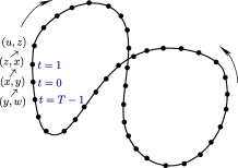
Figure 1: Scheme of an asymmetric limit cycle $\mathcal{C}$; if a configuration $(x,y)$ belongs to $\mathcal{C}$, then $(y,x)$ does not.

Next, we continue with a key property of the Q2R model that will allow to have an easy understanding of the attractor classification shown in this paper.

3.2 Fundamental property between configurations and its symmetrical

The following Reversibility Lemma shows a main characteristic of the Q2R system (2.2).

Lemma 3.16 (Reversibility).

Let $x$, $y$, $z$ in $\Omega$, then,

$$[\left(x,y\right)\to\left(z,x\right)]\Leftrightarrow[\left(x,z\right)\to\left(y,x\right)].$$

Proof.

From (2.2) and because of $\phi\left(x\right)\odot\phi\left(x\right)=\mathbb{1}$:

$$[\left(x,y\right)\to\left(z,x\right)] \Leftrightarrow \left\{\begin{array}[]{l}x=x\\ z=y\odot\phi\left(x\right)\end{array}\right.$$ (3.3)

$$\Leftrightarrow \left\{\begin{array}[]{rl}x&=x\\ z\odot\phi\left(x\right)&=y\end{array}\right.$$

$$\Leftrightarrow [\left(x,z\right)\to\left(y,x\right)]$$

∎

This Reversibility Lemma says that, if there is a one time step evolution between two configurations, then, there is also a one time step evolution between their symmetric configuration, but, in the opposite sense. As a consequence, we have the following generalization:

Corollary 3.17.

Let $x^{t}$, $y^{t}$ in $\Omega$, $t\in\{0,...,p\}$, $p\in\mathbb{N}$, then,

$$\left(x^{0},y^{0}\right)\to\cdots\to(x^{p},y^{p})\Leftrightarrow(y^{p},x^{p})\to\cdots\to\left(y^{0},x^{0}\right).$$

Figure 2 illustrates the proof of this property.

$$\begin{array}[]{cccc}\underbrace{(x^{0},y^{0})\to\left(x^{1},y^{1}\right)}&\to&\cdots&\underbrace{\to(x^{p},y^{p})}\\ {\Updownarrow}&&\cdots&\Updownarrow\\ \overbrace{(y^{0},x^{0})\leftarrow\left(y^{1},x^{1}\right)}&\leftarrow&\cdots&\overbrace{\leftarrow(y^{p},x^{p})}$$\end{array}$$

Figure 2: Applying successively the Lemma 3.16 at each step-evolution $(x^{t},y^{t})\to(x^{t+1},y^{t+1})$, for $t\in\{0,\dots,{p}\}$, $p\in\mathbb{N}$, one constructs the backward evolution between their symmetric configurations.

Let us study the possible evolutions, according to the type of configurations involved.

3.3 The possible evolutions between configurations of type $A$, $B$, $C$ and $D$

Given a configuration of type $U\in\{A,B,C,D\}$, then the only possible evolutions are:

• Configurations of type $A$.
  Let $(x,y)\in A$, then $[x=y]\wedge[\phi(x)=\mathbb{1}]$. Since $\phi(x)=\mathbb{1}$, then $(x,y)\to(y,x)$, and because $y=x$, then $\phi(y)=\mathbb{1}$. Therefore, $(x,x)\to(x,x)\in A$. In fact, this is the characterization of the fixed points of Q2R (Theorem 4.18). Thus, $A\to A$ as shown in Figure 3-(T1).

• Configurations of type $B$.
  Let $(x,y)\in B$, then $[x\neq y]\wedge[\phi(x)=\mathbb{1}]$. Because $\phi(x)=\mathbb{1}$, then $(x,y)\to(y,x)$. Hence, there are two possibilities for $\phi(y)$:

  • If $\phi(y)=\mathbb{1}$, then $(x,y)\to(y,x)\in B$. In fact, this is the characterization of the limit cycles of period two of the Q2R model (Theorem 4.22).

  • If $\phi(y)\neq\mathbb{1}$, then $(x,y)\to(y,x)\in D$.

  Thus, $[B\to B]$ or $[B\to D]$, as shown in Figure 3-(T2).

• Configurations of type $C$.
  Let $(x,y)\in C$, then $[x=y]\wedge[\phi(x)\neq\mathbb{1}]$. Hence, $(x,y)\to(z=y\odot\phi(x),x)$ with $z\neq y$ (consequently, $z\neq x$) and there are two possibilities for $\phi(z)$:

  • If $\phi(z)=\mathbb{1}$, then $(x,y)\to(z,x)\in B$.

  • If $\phi(z)\neq\mathbb{1}$, then $(x,y)\to(z,x)\in D$.

  Thus, $[C\to B]$ or $[C\to D]$, as shown in Figure 3-(T3).

• Configurations of type $D$.
  Let $(x,y)\in D$, then $[x\neq y]\wedge[\phi(x)\neq\mathbb{1}]$. Hence, $(x,y)\to(z=y\odot\phi(x),x)$ with $z\neq y$ (but eventually, $z=x$) and there are two possibilities for $z$, which implies three possible evolutions for $(x,y)$:

  • If $z=x$, then $(x,y)\to(z,x)=(x,x)\in C$.

  • If $z\neq x$, then we have the same two possibilities (T3)-(i) and (T3)-(ii) for $\phi(z)$.

  Therefore, $[D\to B]$, $[D\to C]$ or $[D\to D]$, as shown in Figure 3-(T4).

The above analysis is summarized in Figure 3.

(T1)

(T2)

(T3)

(T4)

Figure 3: (T1) A type $A$ configuration only can evolve to itself. (T2)-(T3) Configurations of type $B$ and $C$ can evolve to configurations of type $B$ or $D$. (T4) A type $D$ configuration can evolve to any configuration, excepting the configurations of type $A$.

4 Main Results

4.1 Characterization of fixed points and limit cycles of period two and higher.

Theorem 4.18 (Characterization of fixed points).

Let $(x,y)\in\Omega^{2}$ be a configuration of the Q2R model. Then,

$$(x,y)\in P_{1}\Leftrightarrow[x=y]\wedge[\phi(x)=\mathbb{1}].$$

Proof.

$$(x,y)\in P_{1} \Leftrightarrow [(x,y)\to(x,y)]\text{, by definition of fixed point.}$$

$$\Leftrightarrow \left\{\begin{array}[]{rl}x&=y\\ x&=y\odot\phi(x)\end{array}\right.\text{, by Remark \ref{rem_iter}.}$$

$$\Leftrightarrow [x=y]\wedge[\phi(x)=\mathbb{1}].$$

∎

Remark 4.19.

The above result states that fixed points of the Q2R model are always configurations of type $A$ (see Figure 4-a), i.e., self-symmetric ($(x,x)\in\Omega^{2}_{xx}$) and without null neighborhoods ($\phi(x)=\mathbb{1}$). Hence, $P_{1}=A$.

a)     b)  

Figure 4: a) Scheme for a fixed point (or limit cycle of period 1). b) Scheme for a period-2 limit cycle.

Since Q2R is a reversible system, if a configuration $(x,y)\in\Omega^{2}$ is not a fixed point, then necessarily it belongs to a limit cycle of period 2 or higher. In this context, as a characterization of such a limit cycles, we consider convenient to explicit the next Corollary, which is the negation of Theorem 4.18.

Corollary 4.20.

Let $(x,y)\in\Omega^{2}$ be a configuration of Q2R. Then,

$$(x,y)\text{ belongs in a limit cycle of period 2 or higher}\Leftrightarrow[x\neq y]\vee[\phi(x)\neq\mathbb{1}].$$

Remark 4.21.

The possible evolutions analyzed before implies that the configurations involved in any limit cycle of period 2 or higher are of type $B$, $C$ or $D$ (not A).

4.2 Period 2 limit cycles

Theorem 4.22 (Characterization of limit cycles of period 2).

Let $(x,y)\in\Omega^{2}$ be a configuration of Q2R. Then,

$$(x,y)\in P_{2}\Leftrightarrow[x\neq y]\wedge[\phi(x)=\mathbb{1}]\wedge[\phi(y)=\mathbb{1}].$$

Proof.

$$(x,y)\in P_{2} \Leftrightarrow [(x,y)\to(y\odot\phi(x),x)\to(x,y)]\text{, by definition of }P_{2}.$$ (4.8)

$$\Leftrightarrow [(x,y)\to(y\odot\phi(x),x)]\wedge\begin{array}[]{c}\left\{\begin{array}[]{rl}y&=y\odot\phi(x)\\ x&=x\odot\phi(y\odot\phi(x))\end{array}\right.\\ \text{(by Remark \ref{rem_iter})}\end{array}$$

$$\Leftrightarrow [(x,y)\to(y\odot\phi(x),x)]\wedge\left\{\begin{array}[]{rl}\phi(x)&=\mathbb{1}\\ \phi(y\odot\phi(x))&=\mathbb{1}\end{array}\right.$$ (4.11)

$$\Leftrightarrow [(x,y)\to(y,x)]\wedge\left\{\begin{array}[]{rl}\phi(x)&=\mathbb{1}\\ \phi(y)&=\mathbb{1}\end{array}\right.$$

$$\Leftrightarrow [x\neq y]\wedge[\phi(x)=\mathbb{1}]\wedge[\phi(y)=\mathbb{1}].$$

∎

Remark 4.23.

The above result says that the limit cycles of period 2 consists of configurations $(x,y)$, of type $B$ and with both states, $x$ and $y$, without null neighborhoods (see Figure 4b). Hence, $P_{2}\subset B$.

Observe that there are elements in $B$ which do not belong to $P_{2}$. For instance, take the configuration $(\mathbb{1},x)\in B$ where the state $x\in\Omega$ is composed by a $2\times 2$ block of -1s surrounded by 1s, i.e.,

$$x=\left[\begin{array}[]{cccccccc}1&1&\cdots&\cdots&\cdots&\cdots&1&1\\ 1&\ddots&\cdots&\cdots&\cdots&\cdots&\vdots&1\\ 1&\ddots&1&1&1&1&\cdots&1\\ \vdots&\cdots&1&-1&-1&1&\cdots&\vdots\\ \vdots&\cdots&1&-1&-1&1&\cdots&\vdots\\ 1&\cdots&1&1&1&1&\cdots&1\\ \vdots&\vdots&\cdots&\cdots&\cdots&\cdots&\ddots&1\\ 1&1&\cdots&\cdots&\cdots&\cdots&1&1\end{array}\right]_{L\times L},$$

This configuration has only 4 null neighborhoods, located just in the nodes of the inner block of -1s. In other words, $\phi(x)=x$. Thus, by applying the Q2R rule we get :

• $(\mathbb{1},x)\to(\phi(\mathbb{1})\odot x,\mathbb{1})=(x,\mathbb{1})$

• $(x,\mathbb{1})\to(\phi(x)\odot\mathbb{1},x)=(x\odot\mathbb{1},x)=(x,x)$

• $(x,x)\to(x\odot\phi(x),x)=(x\odot x,x)=(\mathbb{1},x)$

Therefore, the sequence of evolutions $(\mathbb{1},x)\to(x,\mathbb{1})\to(x,x)\to(\mathbb{1},x)$ is a period-3 limit cycle and, consequently, $(\mathbb{1},x)\in P_{3}$, hence, $(\mathbb{1},x)\notin P_{2}$.

4.3 Period 3 limit cycles

Theorem 4.24 (Characterization of limit cycles of period 3).

Let $\{(x,y),(z,x),(y,z)\}\subset\Omega^{2}$ such that $(x,y)\to(z,x)\to(y,z)$. Then,

$$\{(x,y),(z,x),(y,z)\}\subseteq P_{3}\Leftrightarrow\phi(x)\odot\phi(y)\odot\phi(z)=\mathbb{1}.$$

Proof.

By Remark 2.4, $(x,y)\to(z,x)\to(y,z)$ means that:

$$\underbrace{[y=x\odot\phi(z)]}_{(a)}\wedge\underbrace{[z=y\odot\phi(x)]}_{(b)}$$

$\Rightarrow)$

$$\{(x,y),(z,x),(y,z)\}\subseteq P_{3} \Rightarrow [(y,z)\to(x,y)]$$ (4.15)

$$\Rightarrow x=z\odot\phi(y)\text{, by Remark \ref{rem_iter}.}$$

Replacing (a) in (b) and, after that, (b) in (4.15) we have that $x\odot\phi(x)\odot\phi(y)\odot\phi(z)=x$, i.e.,

$$\phi(x)\odot\phi(y)\odot\phi(z)=\mathbb{1}.$$

$\Leftarrow)$

$$\phi(x)\odot\phi(y)\odot\phi(z)=\mathbb{1} \Rightarrow x\odot\phi(x)\odot\phi(y)\odot\phi(z)=\mathbb{1}\odot x=x$$

$$\Rightarrow [x\odot\phi(z)]\odot\phi(x)\odot\phi(y)=x$$

$$\Rightarrow y\odot\phi(x)\odot\phi(y)=x\text{, by { (a)}.}$$

$$\Rightarrow z\odot\phi(y)=x\text{, by { (b)}.}$$

$$\Rightarrow [(y,z)\to(x,y)]$$

Thus, $[(x,y)\to(z,x)\to(y,z)]\wedge[(y,z)\to(x,y)]$, i.e.,

$$\{(x,y),(z,x),(y,z)\}\subseteq P_{3}$$

∎

Remark 4.25.

Contrary with the statements of the Remarks 4.19 and 4.23, in which fixed points and period-2 limit cycles are shown to have a unique topology, the condition $\phi(x)\odot\phi(y)\odot\phi(z)=\mathbb{1}$ for period-3 limit cycles allows different topologies (see Figure 5). This fact occurs for all limit cycles of period 3 and higher and it will be explained later in Remark 4.29.

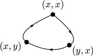
a)     b) 

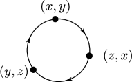
Figure 5: The two different topologies for a period-3 limit cycle: a) A symmetric limit cycle, with one self-symmetric configuration $(x,x)$. b) An asymmetric limit cycle, hence, without any self-symmetric configuration.

4.4 Properties of the configurations in limit cycles with period three and higher.

The following result will be useful for the proof of our main Theorem 4.28 (on the attractors classification in Q2R) and dictates direct consequences that are easily deduced from Theorems 4.18 and 4.22 and the possible evolutions shown in Figure 3.

Corollary 4.26.

Let $\mathcal{C}$ be a limit cycle of Q2R with period 3 or higher. Then:

• $\mathcal{C}$ has at least one configuration of type $D$.

• $\mathcal{C}$ does not have evolutions of type $A\to A$, nor $B\to B$ (notice that $C\to C$ does not exist) but it could have evolutions of type $D\to D$.

• If $\mathcal{C}$ has a type $D$ configuration, then $D$ comes from a type $V$ configuration with $V\in\{B,C,D\}$.

• If $\mathcal{C}$ has a configuration $(x,y)\in B$, then $(x,y)\to(y,x)\in D$.

4.5 Topological classification of limit cycles in Q2R

Definition 4.27.

Let $\mathcal{C}$ be a limit cycle of the Q2R model with period $T\in\mathbb{N}$. We say that $\mathcal{C}$ is:

• A symmetric limit cycle of type I (S-I). If $T=1$ or if there exists $p\in\mathbb{N}_{0}$ such that $\mathcal{C}$ has the topology of Figure 6-a, i.e., is symmetric with:

  • An odd period $T=2(p+1)+1$.

  • Only one configuration of type $C$, only one configuration of type $B$ and $(2p+1)$ configurations of type $D$.

• A symmetric limit cycle of type II (S-II). If there exists $p\in\mathbb{N}_{0}$ such that $\mathcal{C}$ has the topology of Figure 6-b, i.e., is symmetric with:

  • An even period $T=2(p+2)$.

  • Only two configurations of type $C$ and $2(p+1)$ configurations of type $D$.

• A symmetric limit cycle of type III (S-III). If $T=2$ or if there exists $p\in\mathbb{N}_{0}$ such that $\mathcal{C}$ has the topology of Figure 6-c, i.e., is symmetric with:

  • An even period $T=2(p+2)$.

  • Only two type $B$ configurations and $2(p+1)$ type $D$ configurations.

• An asymmetric limit cycle (AS). If there exists $p\in\mathbb{N}\setminus\{1\}$ such that $\mathcal{C}$ has the topology of one of the two limit cycles of Figure 6-d, i.e., is an asymmetric limit cycle with:

  • Period $T=p+1$ (it can be even or odd, depending on the value of $p$).

  • All its configurations are of type $D$.

a)  b)
c)  d)

Figure 6: Topology of different type of limit cycles. a) Symmetric limit cycle of type I. b) Symmetric limit cycle of type II. c) Symmetric limit cycle of type III. d) Two asymmetric limit cycles.

4.6 Attractors classification of Q2R

The following (main) Theorem shows that the only possible limit cycles existing in Q2R are the four ones defined above.

Theorem 4.28 (Attractors classification of Q2R).

Let $\mathcal{C}$ be a limit cycle of Q2R with period $T\in\mathbb{N}$. Then $\mathcal{C}$ is of type S-I, S-II, S-III or AS.

Proof.

Let $\mathcal{C}$ be a limit cycle of Q2R with period $T\in\mathbb{N}$.
If $T=1$ or $T=2$ then, by definition, $\mathcal{C}$ is of type S-I or S-III, respectively.
Let $T\geq 3$, then, by Corollary 4.26-(i), $\mathcal{C}$ has at least one configuration of the type $D$, $(x^{0},y^{0})$, which, according with Corollary 4.26-(iii), it may come from a configuration of the type $B$, $C$ or $D$. Previous statement allows us to consider only three cases for the limit cycle $\mathcal{C}$:

• $\mathcal{C}$ has only configurations of type $D$. In this case, $\mathcal{C}$ has the form $(x^{0},y^{0})\to(x^{1},y^{1})\to\cdots\to(x^{p},y^{p})\to(x^{0},y^{0})$ with $p=T-1$ as in Figure 6d)-right, i.e., $\mathcal{C}$ is of type AS.

• $\mathcal{C}$ has a configuration $(x^{0},y^{0})\in D$ coming from a configuration $(y^{0},x^{0})\in B$, as in Figures 6-a) or 6c). Because of Corollary 4.26-(ii), a configuration of type $D$ could (eventually) evolve to another configuration of type $D$, so, we can consider $p\in\mathbb{N}_{0}$ as the maximum time step such that $[(x^{0},y^{0})\to(x^{1},y^{1})\to\cdots\to(x^{p},y^{p})]\in\mathcal{C}$ and $(x^{t},y^{t})\in D$, $\forall i\in\{0,...,p\}$. Hence, we have only two possible evolutions for the configuration $(x^{p},y^{p})\in D$:

  • $(x^{p},y^{p})\to(x^{p+1},y^{p+1})\in B$.
    In this case, by Corollary 4.26-(iv), $(x^{p+1},y^{p+1})\to(y^{p+1},x^{p+1})\in D$ and $(y^{p+1},x^{p+1})\to(y^{p},x^{p})\to\cdots\to(y^{1},x^{1})\to(y^{0},x^{0})$ (by Corollary 3.17), completing $\mathcal{C}$ with an even period $T=2(p+2)$ as shown in Figure 6c), i.e., $\mathcal{C}$ is of type S-III.

  • $(x^{p},y^{p})\to(x^{p+1},y^{p+1})\in C$.
    In this case, $(x^{p+1},y^{p+1})=(x^{p},x^{p})$ and, again, the Corollary 3.17 justifies both: $(x^{p},x^{p})\to(y^{p},x^{p})$ and $(y^{p},x^{p})\to(y^{p-1},x^{p-1})\to\cdots\to(y^{1},x^{1})\to(y^{0},x^{0})$, completing $\mathcal{C}$ with an odd period $T=2(p+1)+1$ as shown in Figure 6a), i.e., $\mathcal{C}$ is of type S-I.

• $\mathcal{C}$ has a configuration $(x^{0},y^{0})\in D$ coming from a configuration $(y^{0},y^{0})\in C$. By considering $p\in\mathbb{N}_{0}$ the same as (C2), again we have only two possible evolutions for $(x^{p},y^{p})\in D$: $(x^{p+1},y^{p+1})\in B$ or $(x^{p+1},y^{p+1})\in C$, but the analysis in both cases are similar to (i) and (ii) of the previous case (C2), respectively. In the case (i), $\mathcal{C}$ ends being of type S-I with an odd period $T=2(p+1)+1$ as shown in Figure 6a) while that, for the case (ii), $\mathcal{C}$ ends up being of type S-II with an even period $T=2(p+2)$ as shown in Figure 6b).

∎

Remark 4.29.

Let $\mathcal{C}$ be a limit cycle of Q2R with period $T\in\mathbb{N}$ and $(x,y)\in\mathcal{C}$. Some particular information about $T$ and the configuration $(x,y)$ can help us to deduce the particular type of $\mathcal{C}$. In fact:

• If $T$ is odd, then $\mathcal{C}$ could be of type S-I or AS only. If $T$ is even, then $\mathcal{C}$ could be of type S-II, S-III or AS.

• If $(x,y)\in B$ then, if there exists $(x^{\prime},y^{\prime})\in\mathcal{C}$ such that $[(x^{\prime},y^{\prime})\neq(x,y)]\wedge[(x^{\prime},y^{\prime})\in B]$, then $\mathcal{C}$ is of type S-III, otherwise, $\mathcal{C}$ is of type S-I.

• If $x=y$ (i.e., $(x,y)\in\{A,C\}$), then, if there exists $(x^{\prime},y^{\prime})\in\mathcal{C}$ such that $[(x^{\prime},y^{\prime})\neq(x,y)]\wedge[x^{\prime}=y^{\prime}]$, then $\mathcal{C}$ is of type S-II, otherwise, $\mathcal{C}$ is of type S-I.

Remark 4.30.

The asymmetric limit cycles always appear in pairs (in the sense that all the symmetric configurations of one limit cycle belongs into the other limit cycle). Furthermore, we know that $(x,y)\in D$ means $[x\neq y]\wedge[\phi(x)\neq\mathbb{1}]$ (regardless the value of $\phi(y)$) but, if $(x,y)$ belongs to an asymmetric limit cycle, then $(x,y)\in D$ and, necessarily, $\phi(y)\neq\mathbb{1}$, i.e.,

$$[x\neq y]\wedge[\phi(x)\neq\mathbb{1}]\wedge[\phi(y)\neq\mathbb{1}].$$ (4.16)

The converse relation is not true, i.e., if $(x,y)$ satisfy (4.16) then not necessarily $(x,y)$ belongs to an asymmetric limit cycle (see the limit cycle (7.2) in Appendix 7.3 as a counterexample).

Definition 4.31.

We denote by $\nu_{\rm SI}(T)$, $\nu_{\rm SII}(T)$, $\nu_{\rm SIII}(T)$ and $\nu_{\rm AS}(T)$ as the number of configurations belonging to a limit cycle of period $T$ and of type S-I, S-II, S-III and AS, respectively. Similarly, $n_{\rm SI}(T)$, $n_{\rm SII}(T)$, $n_{\rm SIII}(T)$ and $n_{\rm AS}(T)$ denote the number of limit cycles of period $T$ and type S-I, S-II, S-III and AS, respectively. Notice that:

$$\nu(T) = \nu_{\rm SI}(T)+\nu_{\rm SII}(T)+\nu_{\rm SIII}(T)+\nu_{\rm AS}(T)$$

$$n(T) = n_{\rm SI}(T)+n_{\rm SII}(T)+n_{\rm SIII}(T)+n_{\rm AS}(T)$$

$$n_{q}(T) = \frac{\nu_{q}(T)}{T},\quad\text{with }q\in\{{\rm SI},{\rm SII},{\rm SIII},{\rm AS}\}.$$

The following result shows that the sets S-I and S-II are naturally rare in the whole phase space.

Theorem 4.32.

$\displaystyle\sum_{T\geq 1}\left(n_{\rm SI}(T)+2n_{\rm SII}(T)\right)=|\Omega^{2}_{xx}|=2^{N}$.

Proof.

Because of the third point of Remark 4.29, one has that if $(x,x)\in\Omega^{2}_{xx}$, then, $(x,x)$ belongs only to a cycle of type S-I or S-II. Therefore, this Theorem is true because the limit cycles of type S-I include one configuration in $\Omega^{2}_{xx}$ while that those cycles of type S-II include two configurations in $\Omega^{2}_{xx}$. ∎

4.7 On the size of attractor’s sets: a combinatory approach.

In this section we show that the number of fixed points, $|P_{1}|$, will be the fundamental quantity that determine the size of the different sub-spaces of $\Omega^{2}$. Our starting point relates the neighborhoods of $x\in\Omega$ with those of $-x\in\Omega$.

Proposition 4.33.

Let $x\in\Omega$. Then: $\phi(x)=\mathbb{1}\Leftrightarrow\phi(-x)=\mathbb{1}$.

Proof.

The null neighborhoods of $x\in\Omega$ have two -1’s and two 1’s. This is kept for $-x\in\Omega$, so: $\phi(x)\neq\mathbb{1}\Leftrightarrow\phi(-x)\neq\mathbb{1}$. ∎

The second result relates fixed points with limit cycles of period 2.

Theorem 4.34.

$\{(x,x),(y,y)\}\subseteq P_{1}\Leftrightarrow\{(x,y),(y,x)\}\subseteq P_{2}$

Proof.

$$\{(x,x),(y,y)\}\subseteq P_{1} \Leftrightarrow [x\neq y]\wedge[\phi(x)=\mathbb{1}]\wedge[\phi(y)=\mathbb{1}]\text{, by Theorem \ref{MMM1}.}$$

$$\Leftrightarrow \{(x,y),(y,x)\}\subseteq P_{2}\text{, by Theorem \ref{MMM2}.}$$

∎

As a first consequence of the previous Theorem, we have the following result:

Corollary 4.35.

Let $x\in\Omega$ such that $\phi(x)=\mathbb{1}$. Then, in the Q2R dynamics:

• $(x,x)$ and $(-x,-x)$ are two different fixed points, as well as;

• $(x,-x)\to(-x,x)\to(x,-x)$ is a limit cycle of period 2.

Proof.

Let $x\in\Omega$ such that $\phi(x)=\mathbb{1}$, then, by Theorem 4.18 and Proposition 4.33, $\{(x,x),(-x,-x)\}\subseteq P_{1}$. Therefore, by Theorem 4.34, $\{(x,-x),(-x,x)\}\subseteq P_{2}$. Finally, applying the Q2R rule, we have that $(x,-x)\to(-x,x)\to(x,-x)$ is, in fact, a limit cycle of period 2. ∎

4.8 Size of the sets $P_{1}$, $P_{2}$ and $P_{3}$.

A second consequence of Theorem 4.34 shows that the number of limit cycles of period 2 is larger than the number of fixed points, moreover:

Corollary 4.36.

$|P_{2}|=|P_{1}|(|P_{1}|-1)$.

Proof.

$$|P_{2}| = 2\cdot\text{(number of limit cycles of period 2), by definition of }P_{2}$$

$$= 2\cdot{|P_{1}|\choose 2}\text{, by Theorem \ref{thm_fp-cl2}}$$

$$= |P_{1}|(|P_{1}|-1).$$

∎

Moreover, because of Remark 4.19, $P_{1}=A=\left\{(x,y)\in\Omega_{xx}^{2}/\phi(x)=\mathbb{1}\right\}$. In other words, $P_{1}=\{(x,x)\in\Omega^{2}:\,\phi(x)=\mathbb{1}\}$. Thus, $|P_{1}|=|\Phi_{\mathbb{1}}|$ where $\Phi_{\mathbb{1}}=\left\{x\in\Omega/\phi(x)=\mathbb{1}\right\}$, i.e., $\Phi_{\mathbb{1}}$ is the set of states without null neighborhood.

Definition 4.37.

Let $x\in\Omega$. We define the staggered-state [13] $x_{B}$ as the state $x$ restricted to the nodes ${\bm{k}}\in\{1,...,N\}$ such that $k_{1}+k_{2}$ is even. Analogously is defined the staggered-state $x_{W}$ but for the nodes ${\bm{k}}\in\{1,...,N\}$ such that $k_{1}+k_{2}$ is odd. In other words, $x_{B}$ and $x_{W}$ can be seen as the black and white fields in the “chessboard $x\in\Omega$” respectively, and, such that its superposition – denoted with the $\uplus$ symbol – is $x$, i.e.:

$$x=[x_{B}\uplus x_{W}]\in\Omega.$$

We will use the subindices $(\cdot)_{B}$ and $(\cdot)_{W}$ to refer to the corresponding restriction of the element $(\cdot)$ which we are working in order that:

$$(\cdot)=[(\cdot)_{B}\uplus(\cdot)_{W}]\in\Omega.$$

In particular, we define the chessboard states $\mathbb{1}_{BW}$ and $\mathbb{1}_{WB}$ of $\Omega$ as follows:

$$\mathbb{1}_{BW}\equiv[-\mathbb{1}_{B}]\uplus\mathbb{1}_{W}\quad\text{ and }\quad\mathbb{1}_{WB}\equiv-\mathbb{1}_{BW}=\mathbb{1}_{B}\uplus[-\mathbb{1}_{W}].$$

Remark 4.38.

This construction using the staggered-states is particularly useful in the case of the von Neuman neighborhood. Moreover, in the particular case of $L$ being an odd number, the staggered-states loss its utility (see the first fact of Remark 4.43).

Remark 4.39.

According with the above definition, notice the following statements:

1. $\Omega=\Omega_{B}\uplus\Omega_{W}$.

2. $|\Omega|=2^{N}\Rightarrow|\Omega_{B}|=|\Omega_{W}|=2^{N/2}$.

3. $x\in\Omega\Leftrightarrow[x_{B}\in\Omega_{B}]\wedge[x_{W}\in\Omega_{W}]$.

4. $\phi(\mathbb{1}_{BW})=\phi(\mathbb{1}_{WB})=\mathbb{1}$.

The following two propositions establish conditions for the existence of fixed points and limit cycles of period 2 and 3.

Proposition 4.40.

$\forall L$ even, $4\leq|P_{1}|<|P_{2}|$.

Proof.

Because of definition 2.3 and remark 4.39: $\phi(-\mathbb{1})=\phi(\mathbb{1})=\phi(\mathbb{1}_{BW})=\phi(\mathbb{1}_{WB})=\mathbb{1}$. Hence, by Theorem 4.18:

$$\left\{(\mathbb{1},\mathbb{1}),(-\mathbb{1},-\mathbb{1}),(\mathbb{1}_{BW},\mathbb{1}_{BW}),(\mathbb{1}_{WB},\mathbb{1}_{WB})\right\}\subseteq P_{1},$$

therefore, $4\leq|P_{1}|<|P_{1}|(|P_{1}|-1)=|P_{2}|$ (where the last equality is by Corollary 4.36). ∎

Proposition 4.41.

$\forall L\geq 4$, $|P_{3}|\geq 6N=6L^{2}$.

Proof.

Let $L\geq 4$, and consider an state $x\in\Omega$ of Remark 4.23 where we have proved that $\{(\mathbb{1},x),(x,\mathbb{1}),(x,x)\}\subseteq P_{3}$, i.e., $|P_{3}|\geq 3$.

Because the block of -1s may be situated at any point of $x$, there are $N$ equivalent configurations, moreover, because the inverse configuration $(-\mathbb{1},-x)\in P_{3}$, there are at least $2N$ limit cycles of period 3. Therefore, $|P_{3}|\geq 6N$. ∎

Definition 4.42.

We denote by $B_{\mathbb{1}}$ and $W_{\mathbb{1}}$ as the sets of staggered-states $x_{B}\in\Omega_{B}$ and $x_{W}\in\Omega_{W}$ without null neighborhoods, respectively. That is:

$$B_{\mathbb{1}} =\{u\in\Omega_{B}:\exists x\in\Omega,[x_{B}=u]\wedge[\phi(x)_{W}=\mathbb{1}_{W}]\}$$

$$W_{\mathbb{1}} =\{v\in\Omega_{W}:\exists x\in\Omega,[x_{W}=v]\wedge[\phi(x)_{B}=\mathbb{1}_{B}]\}$$

Example.

Consider the following state $x\in\{-1,1\}^{16}$ and its corresponding state $\phi(x)\in\{-1,1\}^{16}$:

$$x=\left[\begin{array}[]{cccc}\framebox{1}&1&\framebox{1}&1\\ 1&\framebox{-1}&1&\framebox{1}\\ \framebox{1}&1&\framebox{-1}&1\\ 1&\framebox{1}&1&\framebox{1}\\ \end{array}\right]\text{ and }\phi(x)=\left[\begin{array}[]{cccc}1&\framebox{1}&1&\framebox{1}\\ \framebox{1}&1&\framebox{-1}&1\\ 1&\framebox{-1}&1&\framebox{1}\\ \framebox{1}&1&\framebox{1}&1\\ \end{array}\right]$$ (4.25)

The values in the boxes of $x$ correspond to the staggered-state $x_{B}\in\{-1,1\}^{8}$ while the other values that are not in boxes correspond to $x_{W}\in\{-1,1\}^{8}$. Similarly, the values in the boxes of $\phi(x)$ correspond to $\phi(x)_{W}$ and were obtained with the values of $x_{B}$ while the other values, that are not in the boxes of $\phi(x)$, correspond to $\phi(x)_{B}$ and were obtained with the values of $x_{W}$.

Remark 4.43.

The previous example allows us to understand the following facts, that are direct consequences of the above definitions:

1. The neighborhoods in $x_{B}$ are independent of those in $x_{W}$, when $L$ is even.

2. $\phi(x)=\mathbb{1}\Leftrightarrow[\phi(x)_{B}=\mathbb{1}_{B}]\wedge[\phi(x)_{W}=\mathbb{1}_{W}]$. In other words, studying the set $\Phi_{\mathbb{1}}$ is equivalent to study the sets $B_{\mathbb{1}}$ and $W_{\mathbb{1}}$.

3. $B_{\mathbb{1}}\uplus W_{\mathbb{1}}=\Phi_{\mathbb{1}}$.

4. $|B_{\mathbb{1}}|=|W_{\mathbb{1}}|$.

Definition 4.44.

We denote $\beta\equiv|B_{\mathbb{1}}|=|W_{\mathbb{1}}|$.

The following corollary will be useful to prove, in Theorem 4.46, that $\beta$ is an even number.

Corollary 4.45.

Let $x\in\Omega$. Then:

1. $x_{B}\in B_{\mathbb{1}}\Leftrightarrow-x_{B}\in B_{\mathbb{1}}$

2. $x_{W}\in W_{\mathbb{1}}\Leftrightarrow-x_{W}\in W_{\mathbb{1}}$

Proof.

Let $x\in\Omega$.

$$(1)\qquad\quad x_{B}\in B_{\mathbb{1}} \Leftrightarrow \phi(x)_{W}=\mathbb{1}_{W}$$

$$\Leftrightarrow \phi(-x)_{W}=\mathbb{1}_{W}$$

(by Proposition 4.33 and fact (2) of Remark 4.43)

$$\Leftrightarrow -x_{B}\in B_{\mathbb{1}}$$

(2) Is analogous to (1). ∎

The following Theorem shows that the number of fixed points of Q2R is always an square number and a multiple of 4.

Theorem 4.46.

The following statements are true:

1. $\beta=2k$, for some $k\in\mathbb{N}$.

2. $|P_{1}|=|\Phi_{\mathbb{1}}|=\beta^{2}=4k^{2}$.

3. $|P_{2}|=4k^{2}(4k^{2}-1)$.

Proof.

1. $\beta\geq 2$ because always $\{\mathbb{1}_{B},-\mathbb{1}_{B}\}\subseteq B_{\mathbb{1}}$ and $\{\mathbb{1}_{W},-\mathbb{1}_{W}\}\subseteq W_{\mathbb{1}}$. The fact that $\beta$ it is even is direct from Corollary 4.45.

2. As already said:
   $|P_{1}|=|\{(x,x)\in\Omega^{2}:\,\phi(x)=\mathbb{1}\}|=|\{x\in\Omega/\phi(x)=\mathbb{1}\}|=|\Phi_{\mathbb{1}}|$. Since $\beta=2k$ and because of the facts (3) and (4) of Remark 4.43: $|\Phi_{\mathbb{1}}|=|B_{\mathbb{1}}|\cdot|W_{\mathbb{1}}|=\beta^{2}=4k^{2}$. Therefore: $|P_{1}|=|\Phi_{\mathbb{1}}|=\beta^{2}=4k^{2}$, for some $k\in\mathbb{N}$.

3. This proof is a direct from Corollary 4.36 and statement (2) previously proved.

∎

5 A general overview of the phase space

Before concluding, we will explain the Figure 7 that summarizes briefly the phase space partitions in limit cycles accordingly with the main results obtained in the previous sections.

• The whole figure represents $\Omega^{2}$ that is partitioned according to definition 3.9: $\Omega^{2}=\Omega_{xx}^{2}\cup\Omega_{xy}^{2}$.

• $\Omega_{xx}^{2}$ (colored by yellow and green) is partitioned in ${A=}P_{1}$ (yellow) and ${C=}\Omega_{xx}^{2}-P_{1}$ (green).

• $\Omega_{xy}^{2}$ (colored by orange and blue) is partitioned in $P_{2}$ (orange) and $\Omega_{xy}^{2}-P_{2}$ (blue).

• The figure tries to reflect, though not in the real scale, that $|\Omega_{xx}^{2}|\ll|\Omega_{xy}^{2}|$ and $|P_{1}|\ll|P_{2}|$.

• $P_{1}\cup P_{2}$ (yellow and orange) represents the set of configurations without null neighborhoods. For the complementary configurations (those of green and blue regions), at least one of its states has a null neighborhood.

• The dashed line, that limits the left region of $\Omega^{2}$ with colors orange, yellow, green and a part of the blue, corresponds to configurations that are symmetric limit cycles (i.e. , limit cycles of type S-I, S-II or S-III only). The remaining region of $\Omega^{2}$ (only in blue) correspond to configurations belonging to asymmetric limit cycles (i.e., of type AS).

• Configurations belonging in $C=\Omega_{xx}^{2}-P_{1}$ (green) are in limit cycles of type S-I or S-II only. Those of type S-I are represented only with one configuration in the green region (the remaining configurations lying in the blue region limited by the dashed line). Those of type S-II are represented only with two configurations in the green region (the remaining configurations lying in the blue region enclosed by the dashed line).

• The limit cycles with all its configurations belonging to the leftmost blue region limited by the dashed line are exclusively of type S-III.

• While $P_{1}$ and $P_{2}$ are exactly the yellow and orange regions, respectively, the other sets $P_{j}$ ($j\geq 3$) have configurations in the green or blue regions (but not in the yellow nor the orange) as exemplified in the figure.

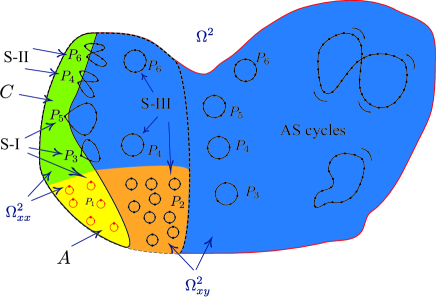
Figure 7: The phase space $\Omega^{2}$ decomposed according to the results of the previous sections.

The following Table 1 complements Figure 7 by showing the sizes of the different regions of $\Omega^{2}$ above mentioned for small system ($N=16,\,32,$ and $64$).

label	variable	size	$L=4$	$L=6$	$L=8$
[b]	$N$	$L^{2}$	16	36	64
[c]	$|\Omega^{2}|$	$2^{2N}$	$2^{32}\sim 4\cdot 10^{9}$	$2^{72}\sim 4\cdot 10^{21}$	$2^{128}\sim 3\cdot 10^{38}$
[d]	$|\Omega_{xx}^{2}|$	$2^{N}$	$2^{16}=65536$	$2^{36}\sim 7\cdot 10^{10}$	$2^{64}\sim 2\cdot 10^{19}$
[e]	$|\Omega_{xy}^{2}|$	[c]-[d]	$\sim 4\cdot 10^{9}<$[c]	$\sim 4\cdot 10^{21}<$[c]	$\sim 3\cdot 10^{38}<$[c]
[f]	—Yellow—	$|P_{1}|=\beta^{2}$	$34^{2}$	$584^{2}$	$39426^{2}$
[g]	— Orange—	$|P_{2}|$= [f]([f]-1)	1335180	$\sim 10^{9}$	$\sim 2\cdot 10^{18}$
[h]	—Green—	[d]-[f]	64380	$\sim 7\cdot 10^{10}<$[d]	$\sim 2\cdot 10^{19}<$[d]
[i]	— Blue—	[c]-([f]+[g]+[h])	$\sim 4\cdot 10^{9}<$[e]	$\sim 4\cdot 10^{21}<$[e]	$\sim 3\cdot 10^{38}<$[e]

Table 1: Summary of the sizes of the main regions discussed in the Figure 7. The 1st column labels the values of the “size” column. The 2nd column has the variables and the main regions explained in Figure 7. In the 3rd column are the size formulas for each “variable” of the 2nd column. In the 4th, 5th and 6th columns are the calculations done for $L\in\{4,6,8\}$, respectively.

Since the sizes of the different partitions shown in Figure 7 essentially depends on $\beta$, this value was computationally calculated in Table 1 by generating all the staggered-states $x_{B}\in\Omega_{B}$ without null neighborhoods (i.e., $\phi(x)_{W}=\mathbb{1}$) in order to construct the set $B_{\mathbb{1}}$. This procedure gave us a computable size of $|\Omega_{B}|=2^{N/2}$, for $N=16,\,32,$ and $64$.

6 Discussion

Because of the relevance of an accurate knowledge of the phase space in complex dynamical systems with many degrees of freedom, we attempted a classification of the phase space of the Q2R cellular automaton which is in close connection with the Ising model and its statistical properties. The Q2R model is reversible and essentially all results of the present paper follow after the Lemma 3.16 (on Reversibility). The main results in the present paper are: Theorem 4.28 that shows a fully classification of all Q2R attractors in four types of limit cycles consisting of symmetric and asymmetric ones. Moreover, a general overview of the phase space decomposition has been provided. Besides, some specific results for small period limit cycles are the following: Theorem 4.46 that shows both, that the total number of fixed points is of the form $|P_{1}|=\beta^{2}=4k^{2}$, with $k\in\mathbb{N}$ and that the number of configurations belonging in a period-2 limit cycle is $|P_{2}|=\beta^{2}(\beta^{2}-1)$. Finally, Theorems 4.18, 4.22 and 4.24 as well as Propositions 4.40 and 4.41 characterize the attractors with period lower or equal to 3 and guarantees that almost always will be present in the Q2R dynamics.

We end this paper with the following open remarks:

1. In the context of statistical mechanics it is important to well characterize the phase space restricted to a subset of constant energy. Regarding the above, preliminary numerical simulations show that limit cycles of different periods can have exactly the same level of energy although we have not yet been able to detect common patterns that allow us to characterize them, so, as a future work, we plan to refine the above numerics by using the limit cycle classification presented in this work in order to detect such a patterns.

2. In this new framework, it is evident that the presence of null neighborhoods is determinant for the presence of limit cycles of period 3 or higher and the absence of null neighborhoods, results in fixed points or period-2 limit cycles. In this context, variations of the Q2R model maybe considered for other regular lattices, however, if the neighborhood possesses an odd number of nodes the further dynamics is trivial. More formally,

   Theorem 6.47.

   If the neighborhood considered for the definition of Q2R is composed by an odd number of nodes, then the Q2R dynamic has only fixed points and period-2 limit cycles.

   Proof.

   If the neighborhood has an odd number of nodes, then, given $x\in\Omega$, all its neighborhoods will have more 1s than -1s or vice-versa. In both cases, its sum will never be 0. In other words, $\phi(x)=\mathbb{1}$, $\forall x\in\Omega$. Thus, by Theorems 4.18 and 4.22, the Q2R dynamic will have only fixed points and period-2 limit cycles. ∎

3. Notice that we do not have a mathematical expression for $\beta$. In this context, all numerical values involving $\beta$ in this paper, such as those of Table 1, were obtained checking state by state if they have or not a null-neighborhood.

4. At a computational level, it is important to note that, to make a correct dynamic study of Q2R, initial configurations of both $\Omega_{xx}^{2}$ and $\Omega_{xy}^{2}$ must be considered because if only the first one is considered, then it will never be possible to obtain, for instance, period-2 limit cycles nor asymmetric limit cycles. On the other hand, if only $\Omega_{xy}^{2}$ is considered, then it will never be possible to obtain fixed points.

5. For the dynamical characterization of limit cycles of period-4 and higher, we have not proven general conditions of existence neither we are not able to compute its cardinality, however, a period $T$ limit cycle is characterized by

   $$(x^{0},y^{0})\to(x^{1},y^{1}) \to (x^{2},y^{2})\to\cdots$$

   $$\cdots \to(x^{T-1},y^{T-1})\to(x^{T},y^{T})=(x^{0},y^{0}),$$

   with $x^{1}=y^{0}\odot\phi(x^{0})$, $y^{1}=x^{0}$, $x^{2}=y^{1}\odot\phi(x^{1})$, …  , $x^{T}=y^{T-1}\odot\phi(x^{T-1})=x^{0}$, $y^{T}=x^{T-1}=y^{0}$. Therefore, one concludes the following necessary (but not sufficient) conditions:

   1. For $T$ even, we have two, a priori, independent conditions:

      $$\phi(x^{0})\odot\phi(x^{2})\odot\phi(x^{4})\odot\cdots\odot\phi(x^{T-4})\odot\phi(x^{T-2}) = \mathbb{1}$$

      $$\phi(x^{1})\odot\phi(x^{3})\odot\phi(x^{5})\odot\cdots\odot\phi(x^{T-3})\odot\phi(x^{T-1}) = \mathbb{1}.$$ (6.1)

   2. For an odd period, one has the necessary condition

      $$\phi(x^{0})\odot\phi(x^{1})\odot\phi(x^{2})\odot\cdots\odot\phi(x^{T-2})\odot\phi(x^{T-1}) = \mathbb{1}.$$ (6.2)

   As an example the period four limit cycles posses three different types of limit cycles, the type S-II, the type S-III and the type AS (see Figure 8).

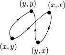
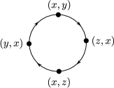
   a)   b)   c)

   
   

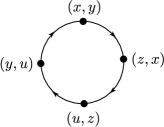
   Figure 8: a) A period-4 limit cycle $(x,x)\to(y,x)\to(y,y)\to(y,x)\to(x,x)$ (type S-II). b) A period-4 limit cycle $(x,y)\to(z,x)\to(x,z)\to(y,x)\to(x,y)$ (type S-III). c) A period-4 limit cycle $(x,y)\to(z,x)\to(u,z)\to(y,u)\to(x,y)$ (type AS).

   The period five limit cycles posses two different types of limit cycles, the type S-I and the type AS (see Figure 9).

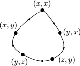
   a)   b)

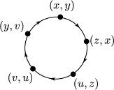
   Figure 9: (a) A period 5 limit cycle $(x,x)\to(y,x)\to(z,y)\to(y,z)\to(x,y)\to(x,x)$. (b) Example of a limit cycle $(x,y)\to(z,x)\to(u,z)\to(v,u)\to(y,v)\to(x,y)$ this limit cycle does not exist in the case of a $4\times 4$ lattice.

6. Because of the special topology of the limit cycles of type S-I and S-II (see Figure 6-a & 6-b) these limit cycles are fully characterized by a simpler set of conditions.

   Let be the sequence:

   $$x^{1} = x^{0}\odot\phi(x^{0})\quad\text{for the first step}$$

   $$x^{t+1} = x^{t-1}\odot\phi(x^{t})\quad\text{ for }\,t=\{1,2,3,\dots,T-1\},$$ (6.3)

   then, the closing conditions for limit cycle for an even periodic limit cycle (6.1) imposes

   $$\phi(x^{0})\odot\phi(x^{1})\odot\phi(x^{2})\odot\phi(x^{3})\odot\cdots\odot\phi(x^{T-4})\odot\phi(x^{T-1}) = \mathbb{1},$$ (6.4)

   while, for an odd period, the condition (6.2) simplifies to

   $$\phi(x^{(T-1)/2}) = \mathbb{1}.$$ (6.5)

   Because the even and odd cases follow quite different conditions we conjecture that:

   Conjecture 6.48.

   Let be odd period $T=2q+1$ with $q\in\mathbb{N}$, and let $x^{1}=x^{0}\odot\phi(x^{0})$, together with $x^{t+1}=x^{t-1}\odot\phi(x^{t})$ for $t\in\{1,2,3,\dots,q-1\}$, then, the pair $(x^{0},x^{0})$ belongs to a type S-I limit cycle of period $T=2q+1$, iff

   $$\phi(x^{0})\neq\mathbb{1}\wedge\phi(x^{1})\neq\mathbb{1}\wedge\dots\wedge\phi(x^{q-1})\neq\mathbb{1}\wedge\phi(x^{q}) = \mathbb{1}.$$

   This condition appears to be an easy way to compute the cardinality of the sets S-I with odd periods.

   Conjecture 6.49.

   Let be the even period $T=2p$, with $p$ a prime number and let $x^{1}=x^{0}\odot\phi(x^{0})$, and $x^{t+1}=x^{t-1}\odot\phi(x^{t})$ for $t=\{1,2,3,\dots,p-2\}$, then the pair $(x^{0},x^{0})$ belongs to a type S-II limit cycle of a period $T=2p$ iff

   $$\phi(x^{0})\neq\mathbb{1}\wedge\phi(x^{1})\neq\mathbb{1}\wedge\dots\wedge\phi(x^{p-2})\neq\mathbb{1}\wedge$$

   $$\phi(x^{0})\odot\phi(x^{1})\odot\dots\odot\phi(x^{p-1}) = \mathbb{1}.$$ (6.6)

   As before, the cardinality of the sets S-II with even periods $T=2p$ ($p$ a prime number), nevertheless, the general even period case requires more careful considerations. Essentially, there is a double counting, e.g. the case of period $T=2\times 4=8$ the condition (6.6) counts simultaneously the period 8 and period 4 configurations.

7 Appendix: Exact results for the case $4\times 4$.

7.1 Decomposition of $\Omega^{2}$

The $4\times 4$ lattice is the largest possible phase space, with $2^{32}$ configurations, that can be fully scanned numerically. The next $6\times 6$ lattice possesses $2^{76}$ configurations, making impossible this task.

In Tables 2 and 3, we provide the exact distributions for the number of configurations and for the number of limit cycles accordingly with its period and the cycle type, respectively. One observes that the number of odd period limit cycles are rare. As a general rule, the number of configurations (and the number of limit cycles) of even period limit cycles are much larger than the odd ones limit cycles. We also notices that the periods 7, 11, 13, etc. are missing. Moreover, the largest odd period is 27. The reason why some periods exist and other does not is still an open problem.

$T$	$\nu_{\rm SI}(T)$	$\nu_{\rm SII}(T)$	$\nu_{\rm SIII}(T)$	$\nu_{\rm AS}(T)$	$|P_{T}|$
1	1,156	0	0	0	1,156
2	0	0	1,335,180	0	1,335,180
3	4,128	0	0	768	4,896
4	0	14,456	20,556,256	48,384,408	68,955,120
5	1,920	0	0	0	1,920
6	0	10,560	15,219,936	20,054,976	35,285,472
8	0	42,752	58,399,744	235,007,232	293,449,728
9	3,456	0	0	4,608	8,064
10	0	7,680	5,174,400	2,941,440	8,123,520
12	0	99,648	132,294,144	655,316,928	787,710,720
18	0	69,120	18,824,832	143,732,736	162,626,688
20	0	19,200	17,295,360	53,694,720	71,009,280
24	0	27,648	115,703,808	536,220,672	651,952,128
27	0	0	0	6,912	6,912
30	0	0	15,851,520	2,949,120	18,800,640
36	0	0	51,038,208	333,388,800	384,427,008
40	0	76,800	26,296,320	246,420,480	272,793,600
54	0	186,624	0	242,721,792	242,908,416
60	0	0	33,177,600	113,172,480	146,350,080
72	0	0	47,333,376	162,201,600	209,534,976
90	0	0	13,271,040	17,694,720	30,965,760
108	0	0	0	329,508,864	329,508,864
120	0	0	0	200,540,160	200,540,160
180	0	0	0	30,965,760	30,965,760
216	0	0	0	179,601,408	179,601,408
270	0	0	0	26,542,080	26,542,080
360	0	0	0	61,931,520	61,931,520
540	0	0	0	26,542,080	26,542,080
1080	0	0	0	53,084,160	53,084,160
Total	10,660	554,488	571,771,724	3,722,630,424	$2^{32}$

Table 2: The distribution of the configurations of $\Omega^{2}$ according with the type of limit cycle that belongs, for a $4\times 4$ periodic lattice. The first column indicates the period-$T$, the second (resp. third, fourth and fifth) one, the total number of configurations belonging in a period-$T$ limit cycle of type S-I (resp. S-II, S-III and AS). Finally, the column $|P_{T}|$ indicates the size of the set $P_{T}$.

$T$	$n_{\rm SI}(T)$	$n_{\rm SII}(T)$	$n_{\rm SIII}(T)$	$n_{\rm AS}(T)$	$n(T)$
1	1,156	0	0	0	1,156
2	0	0	667,590	0	667,590
3	1,376	0	0	256	1,632
4	0	3614	5,139,064	12,096,102	17,238,780
5	384	0	0	0	384
6	0	1,760	2,536,656	3,342,496	5 ,880 ,912
8	0	5,344	7,299,968	29,375,904	36,681,216
9	384	0	0	512	896
10	0	768	517,440	294,144	812,352
12	0	8,304	11,024,512	54,609,744	65,642,560
18	0	3,840	1,045,824	7,985,152	9,034,816
20	0	960	864,768	2,684,736	3,550,464
24	0	1,152	4,820,992	22,342,528	27,164,672
27	0	0	0	256	256
30	0	0	528,384	98,304	626,688
36	0	0	1,417,728	9,260,800	10 ,678 ,528
40	0	1,920	657,408	6,160,512	6,819,840
54	0	3,456	0	4,494,848	4,498,304
60	0	0	552,960	1,886,208	2,439,168
72	0	0	657,408	2,252,800	2,910,208
90	0	0	147,456	196,608	344,064
108	0	0	0	3,051,008	3,051,008
120	0	0	0	1,671,168	1,671,168
180	0	0	0	172,032	172,032
216	0	0	0	831,488	831,488
270	0	0	0	98,304	98,304
360	0	0	0	172,032	172,032
540	0	0	0	49,152	49,152
1080	0	0	0	49,152	49,152
Total	3,300	31,118	37,878,158	163,176,246	201,088,822

Table 3: The distribution of the number of limit cycles for a $4\times 4$ periodic lattice according with its type. The first column indicates the period -$T$, the second (resp. third, fourth and fifth) one, the total number of period-$T$ limit cycles of type S-I (resp. S-II, S-III and AS). Finally, the column $n(T)$ indicates the total number of period-$T$ limit cycles.

The largest number of limit cycles for a given period is obtained for $T=12$ where $n(12)=65,642,560$. The limit cycles of period-12 also correspond with the largest number of configurations, $\nu(12)\approx 787\times 10^{6}$, which is about an $18\%$ of the total phase space. On the contrary, the smallest set is $P_{1}$ with just 1,156 configurations ($\approx 10^{-5}\,\%$). However, Table 3 shows that the smallest number of limit cycles are those of period 27 with 256 limit cycles.

More important, from the total $2^{32}$ configurations, a fraction of $13.33\,\%$ are symmetric limit cycles ($10^{-4}\,\%$ of type S-I, $10^{-2}\,\%$ of type S-II and $13.31\,\%$ of type S-III) and $86.67\,\%$ are asymmetric (AS) limit cycles.

The values showed in the above tables are also summarized in Figure 10 where it can be observed that, apparently, the quantities $\nu_{\rm SI}(T)$, $\nu_{\rm SII}(T)$, $\nu_{\rm SIII}(T)$ and $\nu_{\rm AS}(T)$ (see Figure 10-a) are upper bounded by $K\,T^{-1/2}$, with $K$ a constant. On the contrary the quantities $n_{\rm SI}(T)$, $n_{\rm SII}(T)$, $n_{\rm SIII}(T)$ and $n_{\rm AS}(T)$ (see Figure 10-b) are upper bounded by $K\,T^{-3/2}$ with $K$ a constant. We do not know the reasons for the bound.

Moreover, because of Theorem 4.32 we are able to upper bound the total number of S-I and S-II limit cycles as follows:

$$\sum_{T\geq 1}\left(n_{\rm SI}(T)+n_{\rm SII}(T)\right)<|\Omega^{2}_{xx}|=2^{N}\ll|\Omega^{2}_{xy}|=2^{N}(2^{N}-1).$$

This can be noticed in both Figures 10.

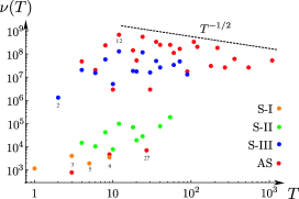
a)  b)

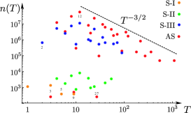
Figure 10: a) Number of configurations, $\nu_{q}(T)$, and (b) number of limit cycles, $n_{q}(T)$, per period, for $q\in\{{\rm SI},{\rm SII},{\rm SIII},{\rm AS}\}$.

Finally, the following Figure 11 plots the normalized density of limit cycles for each topology. To do that, we normalize $n_{\rm SI}(T)$ by $\Omega^{2}_{xx}=2^{N}$, that is

$$\varrho_{\rm SI}(T)=\frac{n_{\rm SI}(T)}{2^{N}}.$$

In the same way we normalize

$$\varrho_{\rm SII}(T)=\frac{2\,n_{\rm SII}(T)}{2^{N}},\quad\varrho_{\rm SIII}(T)=\frac{n_{\rm SII}(T)}{2^{N}(2^{N}-1)},\quad\varrho_{\rm AS}(T)=\frac{n_{\rm AS}(T)}{2^{N}(2^{N}-1)}.$$

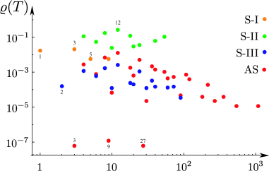
Figure 11: Normalized density of limit cycles per period for different topology.

The interest of this plot is that it shows that relative to its set, namely $\Omega_{xx}^{2}$, the S-I and S-II are of the same order of magnitude, than S-III and AS relative to $\Omega_{xy}^{2}$.

7.2 S-I Example: Limit cycle of odd period

An example of an odd period limit cycle (different of a fixed point) is the following period-3 limit cycle of the form $(x,x)\to(y,x)\to(x,y)\to(x,x)$ (type S-I), like those of Figures 5a) or 6a), where $x$ is in red and $y$ is in blue:

$$\begin{array}[]{ccc}(x,x)=\left({\color[rgb]{1,0,0}\left[\begin{array}[]{cccc}-1&-1&-1&1\\ -1&-1&1&1\\ -1&-1&1&-1\\ -1&-1&1&1\\ \end{array}\right]}\right.&,&\left.{\color[rgb]{1,0,0}\left[\begin{array}[]{cccc}-1&-1&-1&1\\ -1&-1&1&1\\ -1&-1&1&-1\\ -1&-1&1&1\\ \end{array}\right]}\right)\in C\\ (y,x)=\left({\color[rgb]{0,0,1}\left[\begin{array}[]{cccc}-1&-1&-1&-1\\ -1&-1&-1&-1\\ -1&-1&-1&-1\\ -1&-1&-1&-1\\ \end{array}\right]}\right.&,&\left.{\color[rgb]{1,0,0}\left[\begin{array}[]{cccc}-1&-1&-1&1\\ -1&-1&1&1\\ -1&-1&1&-1\\ -1&-1&1&1\\ \end{array}\right]}\right)\in B\\ (x,y)=\left({\color[rgb]{1,0,0}\left[\begin{array}[]{cccc}-1&-1&-1&1\\ -1&-1&1&1\\ -1&-1&1&-1\\ -1&-1&1&1\\ \end{array}\right]}\right.&,&\left.{\color[rgb]{0,0,1}\left[\begin{array}[]{cccc}-1&-1&-1&-1\\ -1&-1&-1&-1\\ -1&-1&-1&-1\\ -1&-1&-1&-1\\ \end{array}\right]}\right)\in D\end{array}$$ (7.1)

Observe that, by Remark 4.29, there not exists limit cycles of type S-I with an even period.

7.3 S-II Example: Limit cycle of even period

The following example is a period-4 limit cycle (type S-II) of the form $(x,x)\to(y,x)\to(y,y)\to(x,y)\to(x,x)$, like those of Figures 6b) or 8a), where $x$ is in red and $y$ is in blue:

$$\begin{array}[]{ccc}(x,x)=\left({\color[rgb]{1,0,0}\left[\begin{array}[]{cccc}1&1&1&1\\ 1&1&1&1\\ 1&1&1&1\\ 1&-1&-1&-1\\ \end{array}\right]}\right.&,&\left.{\color[rgb]{1,0,0}\left[\begin{array}[]{cccc}1&1&1&1\\ 1&1&1&1\\ 1&1&1&1\\ 1&-1&-1&-1\\ \end{array}\right]}\right)\in C\\ (y,x)=\left({\color[rgb]{0,0,1}\left[\begin{array}[]{cccc}1&1&1&1\\ 1&1&1&1\\ 1&1&1&1\\ -1&-1&1&-1\\ \end{array}\right]}\right.&,&\left.{\color[rgb]{1,0,0}\left[\begin{array}[]{cccc}1&1&1&1\\ 1&1&1&1\\ 1&1&1&1\\ 1&-1&-1&-1\\ \end{array}\right]}\right)\in D\\ (y,y)=\left({\color[rgb]{0,0,1}\left[\begin{array}[]{cccc}1&1&1&1\\ 1&1&1&1\\ 1&1&1&1\\ -1&-1&1&-1\\ \end{array}\right]}\right.&,&\left.{\color[rgb]{0,0,1}\left[\begin{array}[]{cccc}1&1&1&1\\ 1&1&1&1\\ 1&1&1&1\\ -1&-1&1&-1\\ \end{array}\right]}\right)\in C\\ (x,y)=\left({\color[rgb]{1,0,0}\left[\begin{array}[]{cccc}1&1&1&1\\ 1&1&1&1\\ 1&1&1&1\\ 1&-1&-1&-1\\ \end{array}\right]}\right.&,&\left.{\color[rgb]{0,0,1}\left[\begin{array}[]{cccc}1&1&1&1\\ 1&1&1&1\\ 1&1&1&1\\ -1&-1&1&-1\\ \end{array}\right]}\right)\in D\\ \end{array}$$ (7.2)

Observe that, by Remark 4.29, there not exists limit cycles of type S-II with an odd period.

7.4 S-III Example: Limit cycle of even period

An example of an even period limit cycle (different of a period-2 limit cycle) is the following period-4 limit cycle of the form $(x,y)\to(z,x)\to(x,z)\to(y,x)\to(x,y)$ (type S-III), like those of the Figures 6c) or 8b), where $x$ is in red, $y$ is in blue and $z$ is in green:

$$\begin{array}[]{ccc}(x,y)=\left({\color[rgb]{1,0,0}\left[\begin{array}[]{cccc}1&1&1&1\\ 1&-1&-1&-1\\ 1&1&-1&1\\ 1&1&1&-1\end{array}\right]}\right.&,&\left.{\color[rgb]{0,0,1}\left[\begin{array}[]{cccc}1&1&1&1\\ 1&1&1&1\\ 1&-1&1&-1\\ -1&1&-1&1\end{array}\right]}\right)\in D\\ (z,x)=\left({\color[rgb]{0,1,0}\left[\begin{array}[]{cccc}1&1&1&-1\\ -1&1&1&1\\ 1&1&1&-1\\ -1&1&1&1\end{array}\right]}\right.&,&\left.{\color[rgb]{1,0,0}\left[\begin{array}[]{cccc}1&1&1&1\\ 1&-1&-1&-1\\ 1&1&-1&1\\ 1&1&1&-1\end{array}\right]}\right)\in B\\ (x,z)=\left({\color[rgb]{1,0,0}\left[\begin{array}[]{cccc}1&1&1&1\\ 1&-1&-1&-1\\ 1&1&-1&1\\ 1&1&1&-1\end{array}\right]}\right.&,&\left.{\color[rgb]{0,1,0}\left[\begin{array}[]{cccc}1&1&1&-1\\ -1&1&1&1\\ 1&1&1&-1\\ -1&1&1&1\end{array}\right]}\right)\in D\\ (y,x)=\left({\color[rgb]{0,0,1}\left[\begin{array}[]{cccc}1&1&1&1\\ 1&1&1&1\\ 1&-1&1&-1\\ -1&1&-1&1\end{array}\right]}\right.&,&\left.{\color[rgb]{1,0,0}\left[\begin{array}[]{cccc}1&1&1&1\\ 1&-1&-1&-1\\ 1&1&-1&1\\ 1&1&1&-1\end{array}\right]}\right)\in B\end{array}$$

Observe that, by Remark 4.29, there not exists limit cycles of type S-III with an odd period.

7.5 AS Example 1: Limit cycle of odd period

The following is a period-3 limit cycle of the form $(x,y)\to(z,x)\to(y,z)\to(x,y)$ (type AS), like those of the Figures 5b) or 6d), where $x$ is in red, $y$ is in blue and $z$ is in green:

$$\begin{array}[]{ccc}(x,y)=\left({\color[rgb]{1,0,0}\left[\begin{array}[]{cccc}-1&1&-1&-1\\ -1&-1&1&-1\\ -1&-1&1&-1\\ -1&1&-1&-1\\ \end{array}\right]}\right.&,&\left.{\color[rgb]{0,0,1}\left[\begin{array}[]{cccc}-1&-1&-1&-1\\ -1&1&1&-1\\ -1&-1&-1&-1\\ -1&1&1&-1\\ \end{array}\right]}\right)\in D\\ (z,x)=\left({\color[rgb]{0,1,0}\left[\begin{array}[]{cccc}-1&-1&1&-1\\ -1&-1&1&-1\\ -1&1&-1&-1\\ -1&1&-1&-1\\ \end{array}\right]}\right.&,&\left.{\color[rgb]{1,0,0}\left[\begin{array}[]{cccc}-1&1&-1&-1\\ -1&-1&1&-1\\ -1&-1&1&-1\\ -1&1&-1&-1\\ \end{array}\right]}\right)\in D\\ (y,z)=\left({\color[rgb]{0,0,1}\left[\begin{array}[]{cccc}-1&-1&-1&-1\\ -1&1&1&-1\\ -1&-1&-1&-1\\ -1&1&1&-1\\ \end{array}\right]}\right.&,&\left.{\color[rgb]{0,1,0}\left[\begin{array}[]{cccc}-1&-1&1&-1\\ -1&-1&1&-1\\ -1&1&-1&-1\\ -1&1&-1&-1\\ \end{array}\right]}\right)\in D\\ \end{array}$$

7.6 AS Example 2: Limit cycle of even period

The following ia a period-4 limit cycle of the form $(x,y)\to(z,x)\to(u,z)\to(y,u)\to(x,y)$ (type AS), like those of the Figures 6d) or 8c), where $x$ is in red, $y$ is in blue, $z$ is in green and $u$ is in black:

$$\begin{array}[]{ccc}(x,y)=\left({\color[rgb]{1,0,0}\left[\begin{array}[]{cccc}1&1&1&1\\ 1&1&1&-1\\ -1&1&-1&1\\ -1&1&1&-1\\ \end{array}\right]}\right.&,&\left.{\color[rgb]{0,0,1}\left[\begin{array}[]{cccc}1&1&1&1\\ 1&1&1&1\\ 1&1&1&1\\ 1&-1&1&-1\\ \end{array}\right]}\right)\in D\\ (z,x)=\left({\color[rgb]{0,1,0}\left[\begin{array}[]{cccc}1&1&1&-1\\ -1&1&-1&1\\ 1&-1&1&1\\ -1&-1&-1&-1\\ \end{array}\right]}\right.&,&\left.{\color[rgb]{1,0,0}\left[\begin{array}[]{cccc}1&1&1&1\\ 1&1&1&-1\\ -1&1&-1&1\\ -1&1&1&-1\\ \end{array}\right]}\right)\in D\\ (u,z)=\left({\left[\begin{array}[]{cccc}1&1&1&1\\ 1&1&1&-1\\ -1&1&-1&1\\ 1&1&-1&-1\\ \end{array}\right]}\right.&,&\left.{\color[rgb]{0,1,0}\left[\begin{array}[]{cccc}1&1&1&-1\\ -1&1&-1&1\\ 1&-1&1&1\\ -1&-1&-1&-1\\ \end{array}\right]}\right)\in D\\ (y,u)=\left({\color[rgb]{0,0,1}\left[\begin{array}[]{cccc}1&1&1&1\\ 1&1&1&1\\ 1&1&1&1\\ 1&-1&1&-1\\ \end{array}\right]}\right.&,&\left.{\left[\begin{array}[]{cccc}1&1&1&1\\ 1&1&1&-1\\ -1&1&-1&1\\ 1&1&-1&-1\\ \end{array}\right]}\right)\in D\\ \end{array}$$

References

- [1] P. Ehrenfest and T. Ehrenfest, Uber eine Aufgabe aus der Warscheinlichkeitsrechnung die mit der kinetischen Deutung der Entropievermehrung zusammenhängt. Math. Naturw. Blätter 3 (1906) 128.
- [2] P. Ehrenfest and T. Ehrenfest, Uber zwei bekannte Einwände gegen das Boltzmannsche H-Theorem? Physikalische Zeitschrift 8 (1907) 311.
- [3] M. Kac, Random walk and the theory of Brownian motion, American Mathematical Monthly 54 (1947), 369.
- [4] A. Puglisi, A. Sarracino and A. Vulpiani, Thermodynamics and Statistical Mechanics of Small Systems, Entropy 20 (2018) 392.
- [5] F. Urbina and S. Rica, Master equation approach to reversible and conservative discrete systems, Phys. Rev. E 94 (2016) 062140.
- [6] G. Vichniac, Simulating Physics with Cellular Automata. Physica D 10 (1984), 96–116.
- [7] Y. Pomeau, Invariant in cellular automata. J. Phys. A: Math. Gen. 17 (1984), L415–L418.
- [8] H. J. Herrmann, H.O. Carmesin and D. Stauffer, Periods and clusters in Ising cellular automata. J. Phys. A: Math. Gen.20 (1987), 4939–4948.
- [9] G. Nicolis and C. Nicolis, Master-equation approach to deterministic chaos. Phys. Rev. A 38 (1988), 427–433.
- [10] K. Lindgren and E. Olbrich, The Approach Towards Equilibrium in a Reversible Ising Dynamics Model: An Information-Theoretic Analysis Based on an Exact Solution, J. Stat. Phys. 168 (2017), 919–935.
- [11] H. Herrmann, Fast algorithm for the simulation of Ising models. J. Stat. Phys. 45 (1986), 145–151.
- [12] E. Goles, and S. Rica, Irreversibility and spontaneous appearance of coherent behavior in reversible systems. Eur. Phys. J. D 62 (2011), 127–137.
- [13] S. Takesue, Staggered Invariants in Cellular Automata. Complex Systems 9 (1995), 149–168.
- [14] P. Grassberger, Long-range effects in an elementary cellular automaton. J. Stat. Phys. 45 (1986), 27–39.
- [15] L. Onsager, Crystal Statistics. I. A Two-Dimensional Model with an Order-Disorder Transition. Phys. Rev. 65 (1944), 117–149.
- [16] C.N. Yang, The Spontaneous Magnetization of a Two-Dimensional Ising Model. Phys. Rev. 85 (1952), 808–816.