Testing the Gravitational Weak Equivalence Principle in the Standard-Model Extension
with Binary Pulsars

Abstract

The Standard-Model Extension provides a framework to systematically investigate possible violation of the Lorentz symmetry. Concerning gravity, the linearized version was extensively examined. We here cast the first set of experimental bounds on the nonlinear terms in the field equation from the anisotropic cubic curvature couplings. These terms introduce body-dependent accelerations for self-gravitating objects, thus violating the gravitational weak equivalence principle (GWEP). Novel phenomena, that are absent in the linearized gravity, remain experimentally unexplored. We constrain them with precise binary-orbit measurements from pulsar timing, wherein the high density and large compactness of neutron stars are crucial for the test. It is the first study that seeks GWEP-violating signals in a fully anisotropic framework with Lorentz violation.

I Introduction

Einstein’s general relativity (GR) is considered as tour de force in describing gravity Einstein (1915); Misner et al. (1973). For the past more than 100 years, GR has passed numerous experimental tests with flying colors Will (2014); Kostelecký and Russell (2011); Wex (2014); Berti et al. (2015); Shao and Wex (2016); Tasson (2014). The wisdom in GR is concisely condensed into the Einstein-Hilbert Lagrangian, ${\cal L}_{\rm EH}=\sqrt{-g}\left(R-2\Lambda\right)/16\pi G$, where $g$ is the determinant of the metric $g_{\mu\nu}$, $R$ is the Ricci scalar, and $\Lambda$ is the cosmological constant. Einstein’s field equations are derived through a variation of ${\cal L}_{\rm EH}$ with respect to $g_{\mu\nu}$. The inherent local Lorentz invariance (LLI) and diffeomorphism symmetry are essential properties for GR from a theoretical viewpoint Kostelecký and Mewes (2018); Misner et al. (1973).

Open questions in the contemporary modern physics, like the very nature of dark matter and dark energy, encourage us to test the underlying fundamental principles in GR. LLI is one of the most important. In a flat spacetime, it links the inertial frames that are relatively moving with respect to each other, while in the curved space, it addresses the property of the tangent space at every single point Misner et al. (1973). However, from a deeper understanding LLI may not be “god-given” Witten (2018), as in string theory Kostelecký and Samuel (1989); Kostelecký and Potting (1991) and loop quantum gravity Gambini and Pullin (1999). Experimental examination, that might either strengthen further our confidence in GR or lead to discoveries beyond the current paradigm, is vital.

The Standard-Model Extension (SME) provides an effective field theory (EFT) that extends our currently well adopted field theories of GR and particle physics. It incorporates all Lorentz-violating (LV) operators which are made out of matter fields and the metric field $g_{\mu\nu}$ Colladay and Kostelecký (1997, 1998); Kostelecký (2004). We call the covariant coupling coefficients the coefficient fields. In this Letter, we focus on the gravity sector of the SME Kostelecký (2004); Bailey and Kostelecký (2006); Bailey et al. (2015); Bailey (2016); Bailey and Havert (2017), and leave LV matter-gravity couplings Kostelecký and Tasson (2011); Jennings et al. (2015) for a future study.

In the SME, conventionally LV operators are sorted according to their mass dimensions as per EFT Kostelecký and Potting (1995); Weinberg (2009). In general, operators with higher mass dimensions are believed to be suppressed. At mass dimension 4, extra coefficient fields in the gravity sector have in total 20 degrees of freedom. Only 9 of them enter the leading-order post-Newtonian (PN) dynamics Bailey and Kostelecký (2006). They are well constrained by various experiments, including lunar laser ranging Battat et al. (2007); Bourgoin et al. (2017), atom interferometers Mueller et al. (2008), cosmic rays Kostelecký and Tasson (2015), pulsar timing Shao (2014a, b), planetary orbital dynamics Hees et al. (2015), super-conducting gravimeters Flowers et al. (2017); Shao et al. (2018), and gravitational waves Abbott et al. (2017) (see Hees et al. (2016) for review). Then at mass dimension 5, new operators introduce a CPT-violating gravitational force. Gravitational waves Kostelecký and Mewes (2016) and binary pulsars Shao and Bailey (2018) were used to put bounds. At mass dimension 6 and higher, short-range experiments in laboratories are extremely powerful to cast useful limits Bailey et al. (2015); Shao et al. (2016); Kostelecký and Mewes (2017); Shao et al. (2019). We refer the reader to the updated data tables Kostelecký and Russell (2011) for details.

Nevertheless, all limits mentioned above are based on the linearized version of gravity Kostelecký and Mewes (2018), where terms are only kept up to the quadratic order of the metric perturbation $h_{\mu\nu}\equiv g_{\mu\nu}-\eta_{\mu\nu}$ in the Lagrangian with $\eta_{\mu\nu}$ being the flat-spacetime metric. After variation with respect to $h_{\mu\nu}$, only linear terms appear in the field equations. The linearized gravity limit unavoidably misses interesting features that only come from nonlinear terms. Bailey (2016) has analyzed an interesting example where the Lagrangian contains a term proportional to the cubic power of the Riemannian tensor $R_{\mu\nu\rho\lambda}$. When restricting to the cubic order of $h_{\mu\nu}$ in the Lagrangian (hence, quadratic order in the field equations), body-dependent effects appear for self-gravitating objects. This is a novel effect for the gravity sector, and it reminds us the well-known Nordtvedt effect Nordtvedt (1968); Will (1993) that is closely related to the gravitational weak equivalence principle (GWEP) Will (1993, 2014); Shao and Wex (2016). In this Letter we analyze this phenomenon in detail with precision binary orbits from pulsar timing Lorimer and Kramer (2005); Wex (2014); Shao et al. (2015), and put the first set of observational bounds.

Unless otherwise stated, we use units where $c=1$.

II Anisotropic cubic curvature couplings

The gravity sector of the SME was built to extend GR by including coefficient fields that couple to the metric and its derivatives Kostelecký (2004). LLI is broken by the cosmological condensation of these coefficient fields. In the 4-dimensional (4d) Riemann-Cartan spacetime, to be compatible with geometrical identities, the breaking should be spontaneous, instead of explicit Kostelecký (2004); Bluhm and Kostelecký (2005). It is set by minimizing the energy of coefficient fields through a Higgs-like mechanism. Nevertheless, unlike the Higgs, coefficient fields can take spacetime indices, thus their nonzero vacuum expectation values (VEVs) break the Lorentz symmetry. In other words, while physical states are LV, the underlying fundamental theory is Lorentz-invariant Tasson (2016).

Being general, the Lagrangian in the SME Kostelecký (2004) reads ${\cal L}={\cal L}_{\rm EH}+{\cal L}_{\rm LV}+{\cal L}_{\rm k}+{\cal L}_{\rm m}$, where (i) ${\cal L}_{\rm m}$ is the matter sector; (ii) ${\cal L}_{\rm k}$ describes the dynamics (including the symmetry breaking) of the coefficient fields, whose details are not crucial here; (iii) ${\cal L}_{\rm LV}$ contains the couplings between the LV coefficient fields with the gravitational field. The terms in ${\cal L}_{\rm k}$ can be organized using the mass dimension of the curvature operator they contain Kostelecký and Potting (1995); Kostelecký (2004); Bailey et al. (2015). As an interesting case study, we focus on operators of mass dimension 8 Bailey (2016),

$${\cal L}^{(8)}_{\rm LV} =\frac{\sqrt{-g}}{16\pi G}k^{(8)}_{\alpha\beta\gamma\delta\kappa\lambda\mu\nu\epsilon\zeta\eta\theta}R^{\alpha\beta\gamma\delta}R^{\kappa\lambda\mu\nu}R^{\epsilon\zeta\eta\theta}\,.$$ (1)

Here $k^{(8)}_{\alpha\beta\gamma\delta\kappa\lambda\mu\nu\epsilon\zeta\eta\theta}$ are the coefficient fields, and they have physical dimensions of quartic length. Like other coefficients, they can be composite of lower-order tensors, as was shown, for example, in Sec. IV of Ref. Bailey and Kostelecký (2006) with bumblebee models. We use the compact grouping notation Bailey (2016), as $k^{(8)}_{\cal ABC}\equiv k^{(8)}_{\alpha\beta\gamma\delta\kappa\lambda\mu\nu\epsilon\zeta\eta\theta}$, $R^{\cal A}R_{\cal A}\equiv R^{\alpha\beta\gamma\delta}R_{\alpha\beta\gamma\delta}$, and so on. By design, when $\left|h_{\mu\nu}\right|\ll 1$, $R^{\alpha\beta\gamma\delta}\sim{\cal O}\left(h\right)$, and ${\cal L}^{(8)}_{\rm LV}\sim{\cal O}\left(h^{3}\right)$. Therefore, the field equations have no ${\cal O}\left(h\right)$ contributions from Eq. (1). Other possible 8d terms proportional to ${\cal D}^{\alpha}{\cal D}^{\beta}R^{\cal A}R^{\cal B}$ and ${\cal D}^{\alpha}{\cal D}^{\beta}{\cal D}^{\gamma}{\cal D}^{\delta}R^{\cal A}$ introduce lower-order contributions of $h$. Therefore, in the sense of solely studying nonlinear terms and body-dependent effects in the gravity sector of the SME, ${\cal L}^{(8)}_{\rm LV}$ is complete at leading order, saving for possible contributions from the dynamical terms in ${\cal L}_{\rm k}$.

Through symmetry breaking, $k^{(8)}_{\cal ABC}$ obtains its VEV, $\bar{k}^{(8)}_{\cal ABC}$. In principle we still need to account for the dynamics of the fluctuation $\tilde{k}^{(8)}_{\cal ABC}\equiv k^{(8)}_{\cal ABC}-\bar{k}^{(8)}_{\cal ABC}$ to be fully compatible with the geometry. However if we restrict to ${\cal O}\left(h^{2}\right)$ terms in the field equation, $\tilde{k}^{(8)}_{\cal ABC}$ does not enter Bailey and Kostelecký (2006); Kostelecký and Tasson (2011); Bailey et al. (2015). Then, after imposing $\partial_{\mu}\bar{k}^{(8)}_{\cal ABC}=0$ in an asymptotically flat Cartesian coordinate, the field equation simply reads Bailey (2016),

$$G_{\mu\nu} =8\pi G\left(T^{\rm m}_{\mu\nu}+T^{\rm k}_{\mu\nu}\right)+6\bar{k}^{(8)}_{\alpha\mu\nu\beta{\cal AB}}\partial^{\alpha}\partial^{\beta}\left(R^{\cal A}R^{\cal B}\right)+{\cal O}\left(h^{3}\right)\,,$$ (2)

where $T^{\rm m}_{\mu\nu}$ and $T^{\rm k}_{\mu\nu}$ are the energy-momentum tensors from ${\cal L}_{\rm m}$ and ${\cal L}_{\rm k}$ respectively. Under mild assumptions on the nature of the dynamical terms for the coefficients $\tilde{k}^{(8)}_{\cal ABC}$, we hereafter neglect the contributions from the stress-energy tensor $T^{\rm k}_{\mu\nu}$. For details on this assumption see section II in Ref. Bailey (2016) and Refs. Seifert (2009); Altschul et al. (2010).

III Binary pulsars

Using the technique of PN calculations Will (1993); Bailey and Kostelecký (2006), it was shown that Bailey (2016), from Eq. (2), the only correction to the PN metric in GR is $\delta h_{00}$ in $h_{00}$ at ${\cal O}\left(v^{4}/c^{4}\right)$. It satisfies a Poisson-like equation Bailey (2016),

$$\nabla^{2}\delta h_{00}=-96\left(\bar{k}^{(8)}_{\rm eff}\right)_{jklmnp}\partial_{j}\partial_{k}\left(\partial_{l}\partial_{m}U\,\partial_{n}\partial_{p}U\right)\,,$$ (3)

where $U$ is the Newtonian potential, and $\bar{k}^{(8)}_{\rm eff}$, with 56 independent components, are linear combinations of $\bar{k}^{(8)}_{\cal ABC}$; see Eq. (17) in Ref. Bailey (2016).

Consider a binary is composed of bodies $a$ and $b$ with masses $m_{a}$ and $m_{b}$. The acceleration for body $a$ is, $\bm{a}_{a}\equiv{\rm d}^{2}\bm{r}_{a}/{\rm d}t^{2}=-Gm_{b}\hat{\bm{n}}/r^{2}+\bm{a}_{a}^{\rm PN}+\delta\bm{a}_{a}$, where $\bm{r}\equiv\bm{r}_{a}-\bm{r}_{b}$ is the separation vector, and $r\equiv\left|\bm{r}\right|$, $\hat{\bm{n}}\equiv\bm{r}/r$. Interchanging indices $a\leftrightarrow b$ gives the acceleration for $b$. The first two terms give the Newtonian and PN accelerations in GR, while the last term is the abnormal acceleration from Eq. (1).

The novel aspect of the abnormal acceleration comes from the dependence on quantities $P_{a}$, $\tilde{P}_{a}$, and $\tilde{P}_{a}^{\prime}$ Bailey (2016),

$$P_{a} \equiv\frac{1}{m_{a}}\int_{a}{\rm d}^{3}\bm{r}\rho_{a}^{2}\,,$$ (4)

$$\tilde{P}_{a} \equiv\frac{1}{35m_{a}}\left(8\pi\int_{a}{\rm d}^{3}\bm{r}\rho_{a}^{2}r^{2}+46\frac{\Omega_{a}}{G}\right)\,,$$ (5)

$$\tilde{P}_{a}^{\prime} \equiv\frac{1}{35m_{a}}\left(16\pi\int_{a}{\rm d}^{3}\bm{r}\rho_{a}^{2}r^{2}-48\frac{\Omega_{a}}{G}\right)\,,$$ (6)

where $\rho_{a}$ and $\Omega_{a}$ are the density and the (Newtonian) gravitational self-energy of body $a$, respectively. The dependence on the internal structure of objects is a distinct feature due to the nonlinear terms coupled to $\bar{k}^{(8)}_{\cal ABC}$’s VEVs Bailey (2016). It is independent of the multipole structure, persisting even in the limit of vanishing multipole moments and tidal forces for perfectly spherical objects. Therefore such a dependence violates the GWEP and generalizes the well-known Nordtvedt effect Nordtvedt (1968); Will (1993); Poisson and Will (2014); Shao and Wex (2016). It is absent in the linearized gravity Bailey and Kostelecký (2006); Kostelecký and Mewes (2018). This interesting feature is our major motivation to study the Lagrangian (1).

Roughly speaking, with a uniform density one has $P_{a}\sim\rho_{a}$ and $\tilde{P}_{a}\sim\tilde{P}_{a}^{\prime}\sim m_{a}/R_{a}$ where $R_{a}$ is the radius of body $a$. The denser of the body (or, the more compact of the body), the larger of these quantities. Pulsars, with their extremely dense nuclear matters and significant compactnesses, fit into this scenario ideally. It is easy to verify that, in a binary system, the denser object dominates the abnormal acceleration. For example, for neutron star–white dwarf (NS-WD) binaries, we only need to consider the GWEP-violating contribution from NSs since WDs are weak-field objects with $\rho_{\rm WD}\ll\rho_{\rm NS}$.

For NSs, the $P_{a}$ contribution is dominant over $\tilde{P}_{a}$ (and $\tilde{P}_{a}^{\prime}$), by $\sim\left(G^{2}m_{b}P_{a}/r^{4}\right)/\left({G^{2}m_{b}\tilde{P}_{a}}/{r^{6}}\right)\sim{r^{2}}/{R_{a}^{2}}\gg 1$. Thus we only need to consider the anomalous acceleration $\propto P_{a}/r^{-4}$. This simplification is not valid for laboratory short-range gravity tests where the separation of bodies is comparable to the size of the objects, and the full Eq. (3) is needed Bailey (2016); Shao et al. (2019).

At the first-order approximation, we assume that the bodies have a uniform density, which introduces a difference $\lesssim 20\%$ in $P_{a}$ with respect to a more realistic density profile. We define an effective radius $\bar{R}$ via, $M/\bar{R}^{3}\equiv m_{a}/R_{a}^{3}+m_{b}/R_{b}^{3}$ where $M\equiv m_{a}+m_{b}$. Thus, we have $\bar{R}\approx R_{\rm NS}$ for NS-NS binaries, and $\bar{R}\approx\left({M}/{m_{\rm NS}}\right)^{1/3}R_{\rm NS}$ for NS-WD binaries. Then the abnormal relative acceleration reads,

$$\delta a^{j}\equiv\delta a^{j}_{a}-\delta a^{j}_{b}\approx-432\frac{\left(GM\right)^{2}}{\bar{R}^{3}}\frac{K_{kl}\hat{n}^{k}\hat{n}^{l}\hat{n}^{j}-\frac{2}{5}K_{jk}\hat{n}^{k}}{r^{4}}\,,$$ (7)

where $K_{jk}$ are linear combinations of $\bar{k}^{(8)}_{\rm eff}$ given in Eq. (37) in Ref. Bailey (2016). It is a symmetric traceless tensor with 5 independent degrees of freedom. $\delta a^{j}$ resembles an effective anisotropic quadrupole moment. However, the Newtonian quadrupole moment decreases when the body gets more compact, while the GWEP-violating effect has the opposite behavior Bailey (2016).

With osculating elements from celestial mechanics Poisson and Will (2014), Bailey (2016) obtained from Eq. (7) the secular changes of orbital elements averaging over a Keplerian orbital period $P_{b}$, $\left\langle{{\rm d}a}/{{\rm d}t}\right\rangle=\left\langle{{\rm d}e}/{{\rm d}t}\right\rangle=0$, and,

$$\left\langle{{\rm d}i}/{{\rm d}t}\right\rangle =2{\cal F}\left(K_{\hat{a}\hat{c}}\cos\omega-K_{\hat{b}\hat{c}}\sin\omega\right)\,,$$ (8)

$$\left\langle{{\rm d}\omega}/{{\rm d}t}\right\rangle ={\cal F}\left[{\cal K}-2\cot i\left(K_{\hat{a}\hat{c}}\sin\omega+K_{\hat{b}\hat{c}}\cos\omega\right)\right]\,,$$ (9)

$$\left\langle{{\rm d}\Omega}/{{\rm d}t}\right\rangle =2{\cal F}\csc i\left(K_{\hat{a}\hat{c}}\sin\omega+K_{\hat{b}\hat{c}}\cos\omega\right)\,,$$ (10)

where we have defined,

$${\cal K} \equiv K_{\hat{a}\hat{a}}+K_{\hat{b}\hat{b}}-2K_{\hat{c}\hat{c}}\,,$$ (11)

$${\cal F} \equiv\frac{216}{5}\frac{n_{b}^{3}a}{\bar{R}^{3}\left(1-e^{2}\right)^{2}}\,.$$ (12)

In the above equations, $a$ is the relative semimajor axis, $e$ is the eccentricity, $i$ is the orbital inclination, $\omega$ is the longitude of periastron, $\Omega$ is the longitude of ascending node, and $n_{b}\equiv 2\pi/P_{b}$ Will (1993); Poisson and Will (2014). $K_{jk}$ is projected onto the coordinate frame $\left(\hat{\bm{a}},\hat{\bm{b}},\hat{\bm{c}}\right)$ attached to the pulsar orbit (see Figure 1 in Ref. Shao (2014b)). The formulae for projections can be found in Eqs. (18–24) in Ref. Shao (2014b).

As in previous work, the change in the orbital inclination is converted to the time derivative of a timing parameter $x_{p}$,

$$\left\langle{\dot{x}_{p}}/{x_{p}}\right\rangle =2{\cal F}\cot i\left(K_{\hat{a}\hat{c}}\cos\omega-K_{\hat{b}\hat{c}}\sin\omega\right)\,,$$ (13)

where $x_{p}\equiv a_{p}\sin i/c$ is the projected semimajor axis for the pulsar orbit with $a_{p}\simeq m_{b}a/M$. We in general do not measure the longitude of ascending node $\Omega$ in pulsar timing unless the pulsar is very nearby Lorimer and Kramer (2005), therefore, we will use the “$\dot{\omega}$-test” in Eq. (9) and the “$\dot{x}_{p}$-test” in Eq. (13) for gravity tests.

From the definition of ${\cal F}$, relativistic binaries with tight orbits (larger $n_{b}^{3}a$) are preferred to the tests; eccentricity increases ${\cal F}$ mildly. We have used a handful of well-timed relativistic binary pulsars to test the CPT-violating gravity Shao and Bailey (2018). Details for these pulsars are provided collectively in Tables I–III in Ref. Shao and Bailey (2018). This collection serves the study here very well. We divide them into 2 groups: (1) the NS-NS group including 4 systems with $P_{b}\lesssim 1$ day: PSRs B1913+16 Weisberg and Huang (2016), B1534+12 Fonseca et al. (2014), B2127+11C Jacoby et al. (2006), and J0737$-$3039A Kramer et al. (2006); (2) the NS-WD group including 7 systems with $P_{b}\lesssim 2$ day: PSRs J0348+0432 Antoniadis et al. (2013), J1738+0333 Freire et al. (2012), J1012+5307 Lazaridis et al. (2009), J0751$+$1807 Desvignes et al. (2016), J1802$-$2124 Ferdman et al. (2010), J1909$-$3744 Desvignes et al. (2016), and J2043+1711 Arzoumanian et al. (2018). The two groups are handled accordingly. The spread in sky location is important to break the parameter degeneracy in the tests, as in the earlier work Shao (2014a, b); Shao and Bailey (2018).

In order to successfully implement the proposed $\dot{\omega}$/$\dot{x}_{p}$ tests, there are some concerns to address. Here we briefly recapitulate a few key points Shao and Bailey (2018); Shao (2014b, a). (i) For pulsars whose $\dot{x}_{p}$ was not reported in literature, we conservatively estimate from the measured uncertainty of $x_{p}$; the estimation was checked independently to be rather good with PSRs B1534+12 and B1913+16 Shao and Bailey (2018). (ii) The unknown $\Omega$ is treated as a nuisance parameter in the Bayesian sense, and a randomization $\Omega\in\left[0,360^{\circ}\right)$ renders our tests as probabilistic tests Tanabashi et al. (2018). (iii) For binaries whose component masses were derived from the accurately measured $\dot{\omega}$ using GR, we recalculate them without using $\dot{\omega}$ (see Ref. Shao and Bailey (2018) for discussions); therefore, we construct “clean” $\dot{\omega}$-tests albeit with a much worse precision. (iv) We take care of the caution that a large $\dot{\omega}$ renders the secular changes nonconstant Wex and Kramer (2007). (v) We handle the fact that a large proper motion for nearby binary pulsars introduces a nonzero $\dot{x}_{p}$ Kopeikin (1996). (vi) A fiducial radius $R_{\rm NS}=12\,$km is used, regardless of the complication from the equation of state.

Table 1: Constraints on the GWEP violation from binary pulsars.

Pulsar	Test	Expression	1$\sigma$ limit $[{\rm km}^{4}]$
J0348+0432	$\dot{x}_{p}$	$\left|0.59K_{\hat{a}\hat{c}}-0.81K_{\hat{b}\hat{c}}\right|$	$<8.2\times 10^{1}$
J0737$-$3039A	$\dot{x}_{p}$	$\left|0.13K_{\hat{a}\hat{c}}-0.99K_{\hat{b}\hat{c}}\right|$	$<4.8\times 10^{3}$
	$\dot{\omega}$	$\left|{\cal K}-0.07K_{\hat{a}\hat{c}}-0.01K_{\hat{b}\hat{c}}\right|$	$<1.2\times 10^{5}$
J0751+1807	$\dot{x}_{p}$	$\left|0.11K_{\hat{a}\hat{c}}-0.99K_{\hat{b}\hat{c}}\right|$	$<3.3\times 10^{2}$
J1012+5307	$\dot{x}_{p}$	$\left|0.39K_{\hat{a}\hat{c}}+0.92K_{\hat{b}\hat{c}}\right|$	$<7.4\times 10^{2}$
B1534+12	$\dot{x}_{p}$	$\left|0.24K_{\hat{a}\hat{c}}+0.97K_{\hat{b}\hat{c}}\right|$	$<4.8\times 10^{2}$
	$\dot{\omega}$	$\left|{\cal K}+0.42K_{\hat{a}\hat{c}}-0.11K_{\hat{b}\hat{c}}\right|$	$<1.7\times 10^{6}$
J1738+0333	$\dot{x}_{p}$	$\left|0.91K_{\hat{a}\hat{c}}+0.41K_{\hat{b}\hat{c}}\right|$	$<1.3\times 10^{2}$
J1802$-$2124	$\dot{x}_{p}$	$\left|0.94K_{\hat{a}\hat{c}}-0.35K_{\hat{b}\hat{c}}\right|$	$<1.5\times 10^{4}$
J1909$-$3744	$\dot{x}_{p}$	$\left|K_{\hat{a}\hat{c}}\right|$	$<5.2\times 10^{3}$
B1913+16	$\dot{x}_{p}$	$\left|0.16K_{\hat{a}\hat{c}}-0.99K_{\hat{b}\hat{c}}\right|$	$<1.3\times 10^{2}$
	$\dot{\omega}$	$\left|{\cal K}+1.8K_{\hat{a}\hat{c}}+0.30K_{\hat{b}\hat{c}}\right|$	$<1.0\times 10^{5}$
J2043+1711	$\dot{x}_{p}$	$\left|0.55K_{\hat{a}\hat{c}}-0.84K_{\hat{b}\hat{c}}\right|$	$<6.7\times 10^{4}$
B2127+11C	$\dot{x}_{p}$	$\left|0.96K_{\hat{a}\hat{c}}+0.29K_{\hat{b}\hat{c}}\right|$	$<6.7\times 10^{3}$
	$\dot{\omega}$	$\left|{\cal K}+0.50K_{\hat{a}\hat{c}}-1.6K_{\hat{b}\hat{c}}\right|$	$<1.7\times 10^{6}$

IV Results

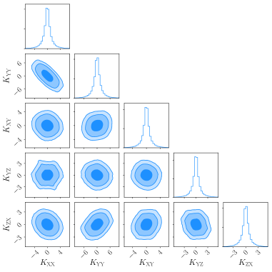
Figure 1: Constraints on $K_{jk}$ in the $\left(\hat{\bf X},\hat{\bf Y},\hat{\bf Z}\right)$ frame. Contours show the 68%, 90%, and 95% CLs. The unit for $K_{jk}$ is $10^{3}\,{\rm km}^{4}$.

After taking the above into account, we have derived 15 independent constraints in Table 1 on various linear combinations of LV coefficients. The pulsars from the NS-WD group provide one $\dot{x}_{p}$-test per system, and those from the NS-NS group provide one $\dot{x}_{p}$-test and one $\dot{\omega}$-test per system. The limits are in the range of ${\cal O}\left(10^{1}\,{\rm km}^{4}\right)$ to ${\cal O}\left(10^{6}\,{\rm km}^{4}\right)$, in a broad agreement with the estimated sensitivity Bailey (2016). In general, the limits from the $\dot{\omega}$-test are worse than those from the $\dot{x}_{p}$-test, due to the large uncertainties in the recalculated masses for the sake of a clean $\dot{\omega}$-test. The tightest limit, $\lesssim 10^{2}\,{\rm km}^{4}$, comes from the $\dot{x}_{p}$ test of PSR J0348+0432.

However, the limits in Table 1 are not expressed in a common coordinate system. They depend on the geometry of binary pulsars through the projections onto the $\left(\hat{\bm{a}},\hat{\bm{b}},\hat{\bm{c}}\right)$ frame. Different binaries carry different frames due to their different sky locations and orbital orientations. To simplify comparisons with other experiments, it is standard to work in the Sun-centered celestial-equatorial coordinate system $\left(\hat{\bf X},\hat{\bf Y},\hat{\bf Z}\right)$ Kostelecký and Mewes (2002); Kostelecký and Russell (2011). As mentioned before, $\left(\hat{\bm{a}},\hat{\bm{b}},\hat{\bm{c}}\right)$ and $\left(\hat{\bf X},\hat{\bf Y},\hat{\bf Z}\right)$ frames are linked by a rotation that composes of 5 simple parts related to the sky location and orbital orientation; see Refs. Shao (2014b); Shao and Bailey (2018) for details. We can relate the components of $K_{jk}$ in these two frames Bailey and Kostelecký (2006) with e.g., $K_{\hat{a}\hat{b}}=K_{jk}\hat{a}^{j}\hat{b}^{k}$ $(j,k={\rm X,Y,Z})$. It allows us to express all limits in Table 1 in terms of $K_{jk}$ in the $\left(\hat{\bf X},\hat{\bf Y},\hat{\bf Z}\right)$ frame and 5 rotation angles $\omega$, $i$, $\Omega$, $\alpha$ (right ascension), and $\delta$ (declination).

Table 2: 1$\sigma$ constraints on $K_{jk}$ in the $\left(\hat{\bf X},\hat{\bf Y},\hat{\bf Z}\right)$ frame.

$K_{jk}$	Scheme A $[{\rm km}^{4}]$	Scheme B $[{\rm km}^{4}]$
$\left|K_{\rm XX}\right|$	$<1.6\times 10^{2}$	$<1.2\times 10^{3}$
$\left|K_{\rm YY}\right|$	$<2.4\times 10^{2}$	$<1.7\times 10^{3}$
$\left|K_{\rm XY}\right|$	$<1.8\times 10^{2}$	$<1.0\times 10^{3}$
$\left|K_{\rm YZ}\right|$	$<1.4\times 10^{2}$	$<8.6\times 10^{2}$
$\left|K_{\rm ZX}\right|$	$<1.6\times 10^{2}$	$<8.8\times 10^{2}$

Table 3: 1$\sigma$ constraints on the absolute values of $\bar{k}^{(8)}_{\rm eff}$ components in Scheme C (unit: ${\rm km}^{4}$). Unconstrained ones are marked with dots.

$\left|{\left(\bar{k}^{(8)}_{\rm eff}\right)}_{\rm XXXXXX}\right|$	$<2.3\times 10^{2}$	$\left|{\left(\bar{k}^{(8)}_{\rm eff}\right)}_{\rm XXXXXY}\right|$	$<1.8\times 10^{2}$
$\left|{\left(\bar{k}^{(8)}_{\rm eff}\right)}_{\rm XXXXXZ}\right|$	$<1.6\times 10^{2}$	$\left|{\left(\bar{k}^{(8)}_{\rm eff}\right)}_{\rm XXXXYY}\right|$	$<5.1\times 10^{2}$
$\left|{\left(\bar{k}^{(8)}_{\rm eff}\right)}_{\rm XXXXYZ}\right|$	$<1.4\times 10^{2}$	$\left|{\left(\bar{k}^{(8)}_{\rm eff}\right)}_{\rm XXXXZZ}\right|$	$<4.1\times 10^{2}$
$\left|{\left(\bar{k}^{(8)}_{\rm eff}\right)}_{\rm XXXYXY}\right|$	$<1.7\times 10^{2}$	$\left|{\left(\bar{k}^{(8)}_{\rm eff}\right)}_{\rm XXXYXZ}\right|$	$\cdots$
$\left|{\left(\bar{k}^{(8)}_{\rm eff}\right)}_{\rm XXXYYY}\right|$	$<2.7\times 10^{2}$	$\left|{\left(\bar{k}^{(8)}_{\rm eff}\right)}_{\rm XXXYYZ}\right|$	$\cdots$
$\left|{\left(\bar{k}^{(8)}_{\rm eff}\right)}_{\rm XXXYZZ}\right|$	$<2.7\times 10^{2}$	$\left|{\left(\bar{k}^{(8)}_{\rm eff}\right)}_{\rm XXXZXZ}\right|$	$<1.7\times 10^{2}$
$\left|{\left(\bar{k}^{(8)}_{\rm eff}\right)}_{\rm XXXZYY}\right|$	$<2.4\times 10^{2}$	$\left|{\left(\bar{k}^{(8)}_{\rm eff}\right)}_{\rm XXXZYZ}\right|$	$\cdots$
$\left|{\left(\bar{k}^{(8)}_{\rm eff}\right)}_{\rm XXXZZZ}\right|$	$<2.4\times 10^{2}$	$\left|{\left(\bar{k}^{(8)}_{\rm eff}\right)}_{\rm XXYYYY}\right|$	$<3.6\times 10^{2}$
$\left|{\left(\bar{k}^{(8)}_{\rm eff}\right)}_{\rm XXYYYZ}\right|$	$<2.1\times 10^{2}$	$\left|{\left(\bar{k}^{(8)}_{\rm eff}\right)}_{\rm XXYYZZ}\right|$	$\cdots$
$\left|{\left(\bar{k}^{(8)}_{\rm eff}\right)}_{\rm XXYZYZ}\right|$	$<1.7\times 10^{2}$	$\left|{\left(\bar{k}^{(8)}_{\rm eff}\right)}_{\rm XXYZZZ}\right|$	$<2.1\times 10^{2}$
$\left|{\left(\bar{k}^{(8)}_{\rm eff}\right)}_{\rm XXZZZZ}\right|$	$<2.8\times 10^{2}$	$\left|{\left(\bar{k}^{(8)}_{\rm eff}\right)}_{\rm XYXYXY}\right|$	$<1.4\times 10^{2}$
$\left|{\left(\bar{k}^{(8)}_{\rm eff}\right)}_{\rm XYXYXZ}\right|$	$<1.2\times 10^{2}$	$\left|{\left(\bar{k}^{(8)}_{\rm eff}\right)}_{\rm XYXYYY}\right|$	$<2.2\times 10^{2}$
$\left|{\left(\bar{k}^{(8)}_{\rm eff}\right)}_{\rm XYXYYZ}\right|$	$<1.1\times 10^{2}$	$\left|{\left(\bar{k}^{(8)}_{\rm eff}\right)}_{\rm XYXYZZ}\right|$	$<3.0\times 10^{2}$
$\left|{\left(\bar{k}^{(8)}_{\rm eff}\right)}_{\rm XYXZXZ}\right|$	$<1.4\times 10^{2}$	$\left|{\left(\bar{k}^{(8)}_{\rm eff}\right)}_{\rm XYXZYY}\right|$	$\cdots$
$\left|{\left(\bar{k}^{(8)}_{\rm eff}\right)}_{\rm XYXZYZ}\right|$	$\cdots$	$\left|{\left(\bar{k}^{(8)}_{\rm eff}\right)}_{\rm XYXZZZ}\right|$	$\cdots$
$\left|{\left(\bar{k}^{(8)}_{\rm eff}\right)}_{\rm XYYYYY}\right|$	$<1.8\times 10^{2}$	$\left|{\left(\bar{k}^{(8)}_{\rm eff}\right)}_{\rm XYYYYZ}\right|$	$\cdots$
$\left|{\left(\bar{k}^{(8)}_{\rm eff}\right)}_{\rm XYYYZZ}\right|$	$<2.7\times 10^{2}$	$\left|{\left(\bar{k}^{(8)}_{\rm eff}\right)}_{\rm XYYZYZ}\right|$	$<1.4\times 10^{2}$
$\left|{\left(\bar{k}^{(8)}_{\rm eff}\right)}_{\rm XYYZZZ}\right|$	$\cdots$	$\left|{\left(\bar{k}^{(8)}_{\rm eff}\right)}_{\rm XYZZZZ}\right|$	$<1.8\times 10^{2}$
$\left|{\left(\bar{k}^{(8)}_{\rm eff}\right)}_{\rm XZXZXZ}\right|$	$<1.2\times 10^{2}$	$\left|{\left(\bar{k}^{(8)}_{\rm eff}\right)}_{\rm XZXZYY}\right|$	$<2.2\times 10^{2}$
$\left|{\left(\bar{k}^{(8)}_{\rm eff}\right)}_{\rm XZXZYZ}\right|$	$<1.1\times 10^{2}$	$\left|{\left(\bar{k}^{(8)}_{\rm eff}\right)}_{\rm XZXZZZ}\right|$	$<3.0\times 10^{2}$
$\left|{\left(\bar{k}^{(8)}_{\rm eff}\right)}_{\rm XZYYYY}\right|$	$<1.6\times 10^{2}$	$\left|{\left(\bar{k}^{(8)}_{\rm eff}\right)}_{\rm XZYYYZ}\right|$	$\cdots$
$\left|{\left(\bar{k}^{(8)}_{\rm eff}\right)}_{\rm XZYYZZ}\right|$	$<2.4\times 10^{2}$	$\left|{\left(\bar{k}^{(8)}_{\rm eff}\right)}_{\rm XZYZYZ}\right|$	$<1.2\times 10^{2}$
$\left|{\left(\bar{k}^{(8)}_{\rm eff}\right)}_{\rm XZYZZZ}\right|$	$\cdots$	$\left|{\left(\bar{k}^{(8)}_{\rm eff}\right)}_{\rm XZZZZZ}\right|$	$<1.6\times 10^{2}$
$\left|{\left(\bar{k}^{(8)}_{\rm eff}\right)}_{\rm YYYYYY}\right|$	$<2.9\times 10^{2}$	$\left|{\left(\bar{k}^{(8)}_{\rm eff}\right)}_{\rm YYYYYZ}\right|$	$<1.4\times 10^{2}$
$\left|{\left(\bar{k}^{(8)}_{\rm eff}\right)}_{\rm YYYYZZ}\right|$	$<2.9\times 10^{2}$	$\left|{\left(\bar{k}^{(8)}_{\rm eff}\right)}_{\rm YYYZYZ}\right|$	$<2.2\times 10^{2}$
$\left|{\left(\bar{k}^{(8)}_{\rm eff}\right)}_{\rm YYYZZZ}\right|$	$<2.1\times 10^{2}$	$\left|{\left(\bar{k}^{(8)}_{\rm eff}\right)}_{\rm YYZZZZ}\right|$	$<2.5\times 10^{2}$
$\left|{\left(\bar{k}^{(8)}_{\rm eff}\right)}_{\rm YZYZYZ}\right|$	$<1.1\times 10^{2}$	$\left|{\left(\bar{k}^{(8)}_{\rm eff}\right)}_{\rm YZYZZZ}\right|$	$<3.0\times 10^{2}$
$\left|{\left(\bar{k}^{(8)}_{\rm eff}\right)}_{\rm YZZZZZ}\right|$	$<1.4\times 10^{2}$	$\left|{\left(\bar{k}^{(8)}_{\rm eff}\right)}_{\rm ZZZZZZ}\right|$	$<4.0\times 10^{2}$

To proceed practically, for a 1$\sigma$ limit “$a$” in Table 1, denoted as $\left|{\cal X}_{a}\left(K_{jk},\Omega_{a}\right)\right|<{\cal C}_{a}$ (e.g., $\left|0.59K_{\hat{a}\hat{c}}-0.81K_{\hat{b}\hat{c}}\right|<8.2\times 10^{1}\,{\rm km}^{4}$ from PSR J0348+0432), we use the following probabilistic density function (PDF) Shao and Bailey (2018),

$$P\left(K_{jk}\right)\propto\prod_{a}\int_{0}^{2\pi}\exp\left\{-\frac{1}{2}\left|\frac{{\cal X}_{a}\left(K_{jk},\Omega_{a}\right)}{{\cal C}_{a}}\right|^{2}\right\}{\rm d}\Omega_{a}\,,$$ (14)

where we have made assumptions on the Gaussianity of measurements and the independence of the limits in Table 1.

We use three schemes to obtain sensible limits on $K_{jk}$. In scheme A, we make an assumption that only one component of $K_{jk}$ in the $\left(\hat{\bf X},\hat{\bf Y},\hat{\bf Z}\right)$ frame is nonzero. We obtain PDF for each component, and extract the limits at 68% CL (see Table 2). The limits are dominated by the tightest limit in Table 1. In scheme B, we allow all components of $K_{jk}$ to be nonzero. We use the emcee package Foreman-Mackey et al. (2013) to investigate their joint PDF with Markov-chain Monte Carlo (MCMC) simulations. We use 20 walkers to accumulate $10^{7}$ samples in total, of which the first half is discarded as the burn-in phase. The 2d pairwise distributions for $K_{jk}$ are shown in Figure 1, together with 1d marginalized distributions. We extract the limits for each component at 68% CL, tabulated in Table 2. We can see that the limits are only worse than those from scheme A by a factor of a few. We have 5 degrees of freedom and 15 constraints. The overconstraining system bounds the values of these 5 components very efficiently Shao (2014a). In scheme C, we assume only one component of $\bar{k}^{(8)}_{\rm eff}$ in the $\left(\hat{\bf X},\hat{\bf Y},\hat{\bf Z}\right)$ frame is nonzero; results are given in Table 3. In this case, we can constrain 45 components of $\bar{k}^{(8)}_{\rm eff}$; the other 11 components do not appear in $K_{jk}$.

The limits in Tables 2 and 3 are the first sets of this kind on the nonlinear terms and body-dependent effects in the gravity sector of the SME. We suggest that other groups can perform similar analysis on their experiments and compare the results with ours. In short-range experiments, a different treatment is needed, and they might probe unconstrained components in this study. We do not make efforts to translate from $K_{jk}$ and $\bar{k}^{(8)}_{\rm eff}$ to $\bar{k}^{(8)}_{\cal ABC}$, because $K_{jk}$ and $\bar{k}^{(8)}_{\rm eff}$ have the actual parameters which appear in the relative acceleration (7) and the Poisson-like equation (3) respectively. It is universal for a variety of experiments, and easy for future comparisons.

V Discussions

In this Letter we follow the theoretical work by Bailey (2016) and investigate in detail the GWEP-violating signals in the gravity sector of the SME with binary pulsars. Nonlinear terms from the anisotropic cubic curvature couplings (1) introduce novel effects that are absent in the linearized gravity. Most notably, the relative accleration between two objects depends on the internal structure of the bodies. The denser the object (or, the more compact the object), the larger the abnormal acceleration. NSs are among the densest objects, hence they are intrinsically privileged in testing this kind of GWEP-violating phenomenon. We use multiple pulsars that were prepared to test the CPT-violating gravity in the SME Shao and Bailey (2018), and put the first sets of bounds on relevant parameters. Our bounds on the GWEP-violating parameters are listed in Tables 2 and 3. We hope other experiments will provide complementary bounds, probably on different degrees of freedom.

The violation of GWEP reminds us the famous “Nordtvedt effect” Nordtvedt (1968). It is one of the main ingredients for the strong equivalence principle (SEP) Will (1993, 2014). For all the valid alternative gravity theories, SEP basically implies the uniqueness of GR Will (2014). Therefore, the tests of the GWEP in this work are important. It provides complementary information to the existing tests of the GWEP in specific alternative gravity theories, like the scalar-tensor gravity Barausse (2017).

It is worthy to mention that, in the theoretical treatment Bailey (2016), we have only used the quadratic ${\cal O}\left(h^{2}\right)$ modifications in the field equation, neglecting all the other higher-order terms. In this sense, our limits should be treated as the strong-field effective limits to their weak-field counterparts; see Refs. Will (2018); Shao and Wex (2012); Shao et al. (2013) for more details. Already at this approximation, we begin to obtain body-dependent GWEP-violating effects. By fully incorporating all the nonlinear terms might provide even more interesting phenomenona. In a class of scalar-tensor gravity, nonperturbative strong-field effects were discovered with fully nonlinear equations Damour and Esposito-Farèse (1993, 1996); Shao et al. (2017); Sennett et al. (2017), that provided important tests for gravitation in the strong-field regime Will (2014); Wex (2014). Possible extension of the gravity sector in the SME to higher orders is beyond the scope of this work.

From the perspective of pulsar timing, continuous observations will improve the $\dot{\omega}$ and $\dot{x}_{p}$ accuracy as $T^{-3/2}$, where $T$ is the observational time span. Thus the $T^{-3/2}$ improvement for $\dot{\omega}$/$\dot{x}_{p}$ tests is guaranteed. The upcoming large radio telescopes and arrays will further tighten the bounds. For example, the Five-hundred-meter Aperture Spherical Telescope (FAST) Nan et al. (2011) and the MeerKAT array Bailes et al. (2018) are starting to operate, and will provide a big improvement in the timing precision. Ultimately for the next decades, the Square Kilometre Array Kramer et al. (2004); Shao et al. (2015); Bull et al. (2018), is going to test gravity in an unparalleled way with its remarkable sensitivity.