GMRT Low-frequency Imaging of an Extended Sample of X-shaped Radio Galaxies

Abstract

We present a low-frequency imaging study of an extended sample of X-shaped radio sources using the Giant Metrewave radio telescope (GMRT) at two frequencies (610 and 240 MHz). The sources were drawn from a Very Large Array FIRST-selected sample and extends an initial GMRT study at the same frequencies, of 12 X-shaped radio galaxies predominantly from the 3CR catalog (Lal & Rao, 2007). Both the intensity maps and spectral index maps of the 16 newly observed sources are presented. With the combined sample of 28 X-shaped radio sources, we found no systematic differences in the spectral properties of the higher surface brightness, active lobes versus the lower surface brightness, off-axis emission. The properties of the combined sample are discussed, including the possible role of a twin active galactic nuclei model in the formation of such objects.

1. Introduction

Morphologically, a small ($\sim$10%) fraction of the general radio galaxy population is comprised of a special class of objects known as X-shaped radio galaxies (Leahy & Parma, 1992; Leahy & Williams, 1984). These objects appear to possess two pairs of radio lobes extending along two distinct axes, unlike the majority of radio galaxies where most of the radio emission is well aligned along a single, primary axis. Thus, a defining characteristic is the presence of synchrotron emitting plasma off the primary axis of the source (Roberts et al., 2018). The more diffuse and lower surface brightness of the two pair of lobes are often termed ‘wings’ or secondary lobes, whereas the higher surface brightness ones are termed active or primary lobes.

A consensus has not been reached regarding the formation mechanism of X-shaped radio sources. There are several models that were proposed for the formation of these objects in the literature. (a) The jet material backflow from the terminal hotspots, therefore they may stream back towards the host galaxy to form the wings of X-shaped sources (Leahy & Williams, 1984). (b) The lobes of a radio galaxy have a lower density than the surrounding medium (Kraft et al., 2005), therefore buoyancy may have an impact on the large-scale morphology of the radio lobes and can form such X-shaped structures (Hodges-Kluck & Reynolds, 2011; Saripalli & Subrahmanyan, 2009; Worrall et al., 1995). Hodges-Kluck & Reynolds (2011); Capetti et al. (2002) invoked a combination of (a, b), first the over-pressured cocoon model for initial expansion and subsequently the buoyancy to explain the observed morphology of X-shaped sources. Capetti et al. (2002) also suggests that jets propagate in an asymmetric enviroment, where the cocoon grows faster in the direction of maximum pressure gradient, generating the wings – this accounts for the observed alignement between the axis of the wings and the minor axis of the host (see also, Gillone, Capetti & Rossi, 2016; Rossi et al., 2017). (c) Parma et al. (1985) suggested precession of the central engine as the formation mechanism of X-shaped radio sources. (d) A reorientation of the jet axis due to a minor merger may also form X-shaped structures (Dennett-Thorpe et al., 2002; Merritt & Ekers, 2002). (e) Lal & Rao (2005, 2007) used the low-frequency spectra from 610/240 MHz data at different locations in the radio structures to understand the nature of these sources and suggested that they could consist of two pairs of jets, which are associated with unresolved binary active galactic nuclei (AGN) system.

Broadly, the above formations models can be categorized as two scenarios, “environmental” (a, b), or due to the central engine (c, d, e). Recently, Saripalli & Roberts (2018) and Roberts et al. (2015) suggested that the X-shaped morphology arises due to a combination of both scenarios, suggesting an interplay of the reorientation of the jet axis and the backflow models. Lal & Rao (2007) studied all the known X-shaped radio sources, predominantly from the 3CR sample and had also pointed out that various X-shaped radio galaxies need not form via a unique formation mechanism, but instead could form via a variety of scenarios which in-turn could explain the differences in the spectral properties of different X-shaped radio galaxies. The earlier studies were based on a small number of objects and Lal & Rao (2007) noted the necessity to improve the statistics.

Table 1Summary of sources and observations.

Object name	Redshift	R. A. (J2000)	Decl. (J2000)	Obs. date	Flux Cal.	Phase Cal.	tint (hrs)
(1)	(2)	(3)	(4)	(5)	(6)	(7)	(8)
J0113$+$0106	0.281	01:13:41.08	$+$01:06:09.0	2006 Dec 25	3C48	3C468.1,	2.91/2.97
						0025$-$260,
						0116$-$208
J0115$-$0000	0.381	01:15:27.33	$-$00:00:01.1	2006 Dec 25	3C48	3C468.1,	3.05/3.05
						0025$-$260,
						0116$-$208
J0702$+$5002	0.094	07:02:47.92	$+$50:02:05.3	2007 Nov 22	3C48	0542$+$498	3.82/3.91
J0859$-$0433	0.356	08:59:50.19	$-$04:33:06.90	2006 Dec 26	3C48,	0834$+$555	2.04/0.58
					3C286
J0914$+$1715	0.520	09:14:05.19	$+$17:15:54.4	2006 Dec 26	3C48,	1021$+$219	2.08/0.67
					3C286
J0917$+$0523	0.591	09:17:44.33	$+$05:23:09.4	2007 Nov 22	3C48	1021$+$219	3.34/3.33
J0924$+$4233	0.2274	09:24:47.01	$+$42:33:47.4	2007 Nov 23	3C147	0834$+$555,	2.88/2.68
						1123$+$055
J1055$-$0707	$-$	10:55:52.56	$-$07:07:19.1	2007 Nov 24	3C286	1123$+$055	2.62/2.62
J1130$+$0058	0.1325	11:30:21.42	$+$00:58:22.9	2006 Dec 26	3C48,	1123$+$055	2.56/2.98
					3C286
J1218$+$1955	0.424	12:18:59.16	$+$19:55:28.0	2006 Dec 26	3C48,	1123$+$055	2.91/3.07
					3C286
J1309$-$0012	0.419	13:09:49.65	$-$00:12:35.2	2006 Dec 24	3C147,	3C468.1,	3.52/3.68
					3C286	1419$+$064
J1339$-$0016	0.1452	13:39:34.26	$-$00:16:35.8	2007 Nov 24	3C147,	1419$+$064	2.63/2.76
					3C286
J1406$-$0154	0.641	14:06:48.63	$-$01:54:17.3	2006 Dec 24	3C147,	3C468.1,	3.46/3.34
					3C286	1419$+$064
J1430$+$5217	0.3671	14:30:17.32	$+$52:17:35.3	2007 Nov 24	3C147,	1419$+$064	2.54/2.76
					3C286
J1600$+$2058	0.1735	16:00:38.94	$+$20:58:51.9	2006 Dec 25	3C48,	1021$+$219,	2.78/1.28
					3C147	1419$+$064,
						1822$-$096
J1606$+$0000	0.059	16:06:12.71	$+$00:00:27.1	2006 Dec 25	3C48,	1021$+$219,	2.81/2.03
					3C147	1419$+$064,
						1822$-$096

In this paper, we extend the Giant Metrewave radio telescope (GMRT) spectral-morphological study of Lal & Rao (2007), who studied all the known winged$/$X-shaped radio sources at the time, predominantly those known from the 3CR catalog. The new targets consist 16 more sources, taken from a sample of 100 candidate X-shaped radio sources using the Very Large Array (VLA) FIRST Becker et al. (1995) survey database (Cheung, 2007). We also include results from the original study of 12 sources (Lal & Rao, 2007), thereby increasing the sample of X-shaped sources to 28 sources, in order to understand the formation scenarios of these sources in a statistical manner. This large sample would be used to understand the relationship, if any, among three categories, (i) where wings have flatter spectra than primary lobes, (ii) where wings and primary lobes have comparable spectral indices and (iii) where wings have steeper spectra than the primary lobes, of X-shaped radio sources.

The paper is organized as follows. The sample selection and GMRT observational details of the 16 sources are given in Sections  2 and 3, respectively. The high-resolution GMRT 610 MHz total intensity maps and the spectral index maps constructed at the lower-resolution corresponding to the 240 MHz data are given in Section  4. The Appendix includes the 240 MHz images together with the lower-resolution versions of the 610 MHz data. Our findings are briefly discussed and summarized in Section 5. Throughout, positions are given in J2000 coordinates.

2. Sample

Cheung (2007) compiled a sample of 100 candidate winged and X-shaped radio sources drawn from the VLA FIRST survey (Becker et al., 1995) database. For our GMRT study, we selected sources amongst these candidates which have (i) characteristic ‘X’ shape based on the $\sim$5^′′ resolution FIRST 1.4 GHz images, (ii) both set of lobes passing symmetrically through the center of the associated host galaxy, and (iii) an angular size greater than 1.2^′ so as to allow more than 7$-$8 synthesized beams across the whole source at the observing frequency (240 MHz) utilized. We additionally observed J1130$+$0058, an X-shaped radio galaxy similarly discovered through its FIRST image (Wang et al., 2003), and satisfied these criteria. The above criteria provided us with a sample comprised of 16 targets listed in Table 1.

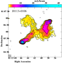
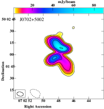
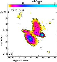
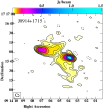
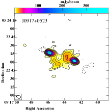
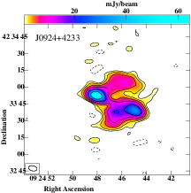
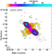
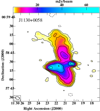
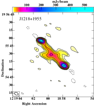
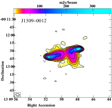
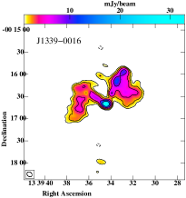
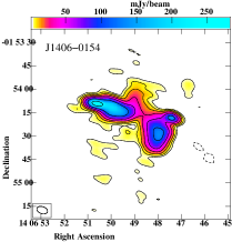
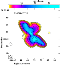
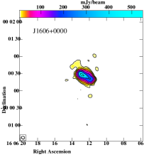
Figure 1.— Full resolution GMRT 610 MHz contour maps for the 16 sample sources, ordered in increasing right ascension from left to right, and then down (see also Table 1). The contour levels and surface brightness peaks are listed in Table 2. The boxed ellipse in the lower left-hand corner shows the shape of the FWHM synthesized beam in each case.

Table 2High-resolution GMRT 610 MHz map parameters presented in Figure 1.

Object name	Beam	P.A.	Peak	rms noise	Contour levels
		(deg.)	(mJy beam-1)
J0113$+$0106	7.1′′ $\times$ 14.2′′	70.2	42.3	0.10	0.5 $\times$ ($-$1, 1, 2, 4, …)
J0115$-$0000	7.9′′ $\times$ 12.0′′	70.9	43.0	0.19	0.8 $\times$ ($-$1, 1, 2, 4, …)
J0702$+$5002	8.4′′ $\times$ 5.2′′	79.4	88.6	0.39	3.0 $\times$ ($-$1, 1, 2, 4, …)
J0859$-$0433	6.7′′ $\times$ 4.6′′	61.1	62.4	0.15	0.9 $\times$ ($-$1, 1, 2, 4, …)
J0914$+$1715	6.6′′ $\times$ 4.3′′	68.9	1505.2	0.39	3.6 $\times$ ($-$1, 1, 2, 4, …)
J0917$+$0523	7.5′′ $\times$ 5.0′′	69.6	389.6	0.25	2.8 $\times$ ($-$2, $-$1, 1, 2, 4, …)
J0924$+$4233	7.7′′ $\times$ 13.9′′	77.0	64.0	0.18	1.6 $\times$ ($-$1, 1, 2, 4, …)
J1055$-$0707	7.0′′ $\times$ 11.2′′	83.0	99.8	0.13	1.1 $\times$ ($-$2, $-$1, 1, 2, 4, …)
J1130$+$0058	7.3′′ $\times$ 4.4′′	77.0	70.3	0.14	0.9 $\times$ ($-$1, 1, 2, 4, …)
J1218$+$1955	7.5′′ $\times$ 11.3′′	73.1	557.6	0.30	3.2 $\times$ ($-$2, $-$1, 1, 2, 4, …)
J1309$-$0012	7.1′′ $\times$ 13.2′′	79.9	367.6	0.37	3.6 $\times$ ($-$1, 1, 2, 4, …)
J1339$-$0016	7.5′′ $\times$ 6.0′′	49.5	32.7	0.10	1.0 $\times$ ($-$1, 1, 2, 4, …)
J1406$-$0154	7.2′′ $\times$ 12.1′′	71.5	280.2	0.30	3.6 $\times$ ($-$1, 1, 2, 4, …)
J1430$+$5217	6.5′′ $\times$ 5.1′′	85.9	241.9	0.23	1.7 $\times$ ($-$1, 1, 2, 4, …)
J1600$+$2058	5.3′′ $\times$ 4.1′′	55.2	37.7	0.06	0.4 $\times$ ($-$1, 1, 2, 4, …)
J1606$+$0000	6.2′′ $\times$ 4.6′′	73.0	545.2	0.84	7.6 $\times$ ($-$1, 1, 2, 4, …)

3. GMRT data and analysis

The 16 sources were observed with the GMRT during two 3-day sessions in December 2006 and November 2007 (see Table 1 for a summary). All observations used the dual frequency mode observing simultaneously at 610 MHz and 240 MHz with bandwidths of 16 MHz and 8 MHz, respectively. To improve ($u,v$) coverage, target scans were obtained over a range of hour angles, interleaved with observations of phase and flux density calibrators. We aimed for $\sim 2-3$ hrs of total exposure obtained per source, before editing.

The data were calibrated as in Lal & Rao (2007). In summary, basic editing of the data, including flagging and calibration was carried out using the flagcal package (Prasad & Chengalur, 2012) with the rest of the analysis performed using the NRAO AIPS package (Bridle & Greisen, 1994). Typically $\lesssim$20% of the data were flagged (predominantly due to radio frequency interference) for each source. Wide fields of view were imaged using facets to map each of the two frequencies for every target. After three to four rounds of phase-only self-calibration, a final self-calibration of both amplitude and phase was performed to obtain the final images. Finally, the facets were stitched and corrected for the primary beam of the GMRT antennas.

4. Results

4.1. Radio Morphology

The high resolution, high sensitivity radio maps of all our 16 X-shaped radio galaxies at 610 MHz are shown in Figure 1 with map parameters given in Table 2. The root mean square (rms) noise measurements were taken in source-free regions away from phase-centre, and are occasionally lower than the local noise levels in the vicinity of our targets. Hence, the first contour-levels are 3–5 $\times$ the rms noise in the vicinity of our targets.

The features observed in these high-resolution GMRT 610 MHz maps have similar resolution and sensitivity to the 5^′′ resolution VLA-FIRST 1.4 GHz images (see Cheung, 2007). In most cases, the radio morphology of the primary lobes can be characterized as having edge-brightened (FR II type; Fanaroff & Riley, 1974) radio structures, confirmed in higher-resolution VLA images (Roberts et al., 2015, 2018). The two exceptions are J0702$+$5002 and J1600$+$2058 with morphology better classified as FR I. J0702$+$5002 is absent of clear hotspots, even in the high-resolution image at 610 MHz in the source, and we take the lobes pointed towards the north-east and south-west direction that have higher peak surface brightness as the primary lobes. Saripalli & Roberts (2018) suggested J1600$+$2058 may be an FRII, but it shows evidence for higher intensity close to the radio core, indicative of an FR I radio galaxy in line with the original classification (Cheung, 2007). We define the north-east and south-west direction as the axis of the primary lobes.

Note that the wings in J1606$+$0000 are barely detected in our GMRT images, although they are clearly seen in the VLA FIRST survey image (Cheung, 2007). Similarly, J1339$-$0016 shows ‘W’-shaped morphology in our 610 MHz map, possibly because the two jets and hence the two primary lobes are bent because the source is moving through the dense gas in the cluster environment (e.g., Hao et al., 2010) We define the northern, high surface brightness regions close to the radio core as the active lobes and southern, low surface brightness regions far away from the radio core as the wings. Both these sources are included in our sample and the inclusion of these two sources do not affect the overall spectral trends we observe over the total sample of 28 objects.

It is also worth mentioning that J0115$-$0000 is a peculiar source and stands out from the rest of X-shaped radio sources studied. In higher-resolution VLA images (Roberts et al., 2018), the edge-brightened inner structure becomes more apparent, particularly in the polarization structure, indicating this is a possible ‘winged double-double’ radio galaxy. Interestingly, the wings identified by Cheung (2007) are apparently connected with the inner lobes in our maps, giving the inner structure an overall ‘Z’-shaped symmetry (Gopal-Krishna et al., 2003) as well.

The lower resolution maps at 240 MHz are shown for the 16 individual sources in the Appendix together with similar (lower) resolution versions of the 610 MHz data (Figure 4). These data were used to create spectral index images, where the final calibrated ($u,v$) data at 610 MHz were re-mapped using a ($u,v$) taper corresponding to the 240-MHz data, giving the beam sizes at these two frequencies that are nearly identical. Both maps were then restored using the circular/symmetric synthesized beam corresponding to the major axis of the beam-shape of the 240 MHz map and corrected for misalignment, if any. Pixels below 5 $\times$ rms were clipped at both frequencies and the spectral index maps were constructed. We use the ratio of log($S_{\rm 240~{}MHz}(x,y)$/$S_{\rm 610~{}MHz}(x,y)$) and log(240 MHz/610 MHz) to construct the spectral index distribution between maps, $S_{\rm 240~{}MHz}(x,y)$ and $S_{\rm 610~{}MHz}(x,y)$.

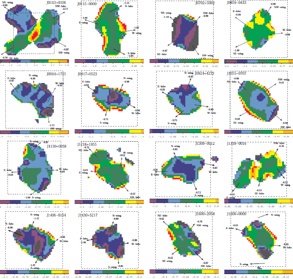
Figure 2.— The maps of our 16 sample sources showing the spatial distribution of the spectral indices between 240 and 610 MHz (color bars), ordered in increasing right ascension as in Figure 1. Dashed lines in each panel indicate 2^′-sided squares.

4.2. Global Spectral Index Properties

The two-frequency spectral index maps for the 16 newly observed X-shaped radio sources are shown in Figure 2. They show remarkable variation across each of the sources. We have shown only a small range of spectral indices for clarity, though the full range is large in each case.

We follow the recipe of Lal & Rao (2007) to determine flux densities at 610 MHz and at 240 MHz and hence the spectral index for the active lobes and the wings using regions defined at their respective locations. This was done for our 16 newly observed X-shaped sources, thereby making this sample consistent in terms of data analysis with the known sample of X-shaped sources observed by Lal & Rao (2007) (maps shown in the lower-right panels of Figures  1–11 therein). Hereagain, the measurements are integrated over the region, which is at least four times the beam size (either a circular region of $\sim$6 pixel radius or a polygon shaped region centered at the position of the tail) and above their 5$\sigma$ surface brightness contour levels to reduce statistical errors (Table 3). Appropriate care was taken when determining the flux density values in the wings and in the active lobes so as to avoid contamination as much as possible. We also tried regions of various sizes and shapes, including irregular polygons, in order to avoid contamination, if any and our results presented here do not change. Unlike Lal & Rao (2007), here we are more conservative with the flux density error values and assume a 5% calibration error, which were added to the rms of the map in quadrature. The calibration error is dominant as compared to error contributed by the rms of the map itself. We recalculate the errors in these maps as well as in Lal & Rao (2007) maps and quote spectral index values after accounting for the calibration errors. This translates to a maximum probable error of 0.06 on the spectral index values.

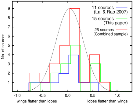
Figure 3.— The distribution of $\Delta{\alpha}$, difference between the averaged spectral indices in the two primary active lobes and the two secondary wings. The three histograms (for clarity, shifted slightly with respect to one another) are for the present sample of 16 candidate X-shaped sources (green), the earlier Lal & Rao (2007) sample (blue), and for the combined sample (red). Also shown is the Gaussian function fit to the combined sample of 28 sources, with a standard deviation, $\sigma$ ($\simeq\pm$0.27). The sources in the central two bins, whose differences in spectral indices are not significant, i.e., $-1\sigma$ $<$ $\Delta{\alpha}$ $<$ $+1\sigma$, are classified as category (ii) sources showing comparable spectral indices for the primary active lobes and the secondary wings. The sources in the left-bins, $\Delta{\alpha}$ $\leq$ $-1\sigma$ are sources with secondary wings to be flatter than the primary active lobes, category (i) and in the right-bins, $\Delta{\alpha}$ $\geq$ $+1\sigma$ are sources with secondary wings to be steeper than the primary active lobes, category (iii).

The radio lobe emission and its spectrum for each of the sample sources is typical of radio lobes of classical FR II source (e.g., Lal, Hardcastle & Kraft, 2008). Though the emission from diffuse wings is similar in surface brightness to the diffuse emission seen in classical FR II sources, but their the spectra are different. Diffuse wings occassionally show flat spectrum in some sources as compared to steep spectra, typically seen in FR II sources. We determine the difference between the averaged spectral indices in the two active (primary) lobes and in the two wings (secondary lobes), $\Delta{\alpha}=\alpha_{\rm primary}-\alpha_{\rm secondary}$, for each source in our earlier observed 12 sources in Lal & Rao (2007) and the 16 X-shaped sources in this paper. Following Lal & Rao (2007), the sample sources can again be categorized into following three groups:

• the secondary, low-surface brightness wings have flatter spectra as compared to the primary active lobes, with $\Delta{\alpha}$ $\leq$ $-1\sigma$,
  

• the secondary, low-surface brightness wings and primary active lobes have comparable spectral indices, with $-1\sigma$ $<$ $\Delta{\alpha}$ $<$ $+1\sigma$, and
  

• the secondary, low-surface brightness wings have steeper spectra as compared to the primary active lobes, with $\Delta{\alpha}$ $\geq$ $+1\sigma$,
  

where, $\sigma$ ($\simeq$ 0.27; see also Figure 3) is the standard deviation, assuming a normal distribution for $\Delta{\alpha}$. Note that we do not include sources J1606$+$0000 and B2 0828$+$28 from our current sample of candidate X-shaped galaxies and from Lal & Rao (2007) known sample of X-shaped galaxies, respectively where we do not have detections for the radio wings.

Table 3Flux densities of the distinct regions, and the spectral indices along with its error estimates in lobes and wings.

Object name	Region	$S_{\nu}$ (mJy)		$\alpha_{\rm 240MHz}^{\rm 610MHz}$
		610	240
J0113$+$0106	SE-lobe	131.4	272.0	$-$0.78 $\pm$0.06
	NW-lobe	75.1	154.1	$-$0.77 $\pm$0.04
	NE-wing	45.7	111.2	$-$0.96 $\pm$0.05
	SW-wing	95.9	215.9	$-$0.87 $\pm$0.10
J0115$-$0000	N-lobe	51.8	148.6	$-$1.13 $\pm$0.06
	S-lobe	44.4	117.1	$-$1.04 $\pm$0.05
	E-wing	21.6	58.1	$-$1.06 $\pm$0.06
	W-wing	18.3	47.4	$-$1.02 $\pm$0.03
J0702$+$5002	SE-lobe	14.6	36.1	$-$0.97 $\pm$0.02
	NW-lobe	17.6	44.4	$-$0.99 $\pm$0.02
	NE-wing	16.1	44.9	$-$1.10 $\pm$0.06
	SW-wing	25.2	80.8	$-$1.25 $\pm$0.10
J0859$-$0433	E-lobe	44.7	109.5	$-$0.96 $\pm$0.04
	W-lobe	41.4	94.1	$-$0.88 $\pm$0.06
	NW-wing	32.1	74.3	$-$0.90 $\pm$0.06
	SE-wing	18.5	46.9	$-$1.00 $\pm$0.10
J0914$+$1715	E-lobe	570.3	1409.5	$-$0.97 $\pm$0.03
	W-lobe	1593.8	3830.3	$-$0.94 $\pm$0.05
	N-wing	72.3	161.3	$-$0.86 $\pm$0.07
	SW-wing	42.2	120.0	$-$1.12 $\pm$0.08
J0917$+$0523	E-lobe	376.1	947.0	$-$0.99 $\pm$0.03
	W-lobe	364.9	893.4	$-$0.96 $\pm$0.04
	N-wing	9.7	24.2	$-$0.98 $\pm$0.07
	S-wing	20.3	39.4	$-$0.71 $\pm$0.04
J0924$+$4233	E-lobe	136.8	296.7	$-$0.83 $\pm$0.02
	W-lobe	98.2	207.1	$-$0.80 $\pm$0.04
	N-wing	36.2	81.5	$-$0.87 $\pm$0.03
	S-wing	16.0	31.6	$-$0.73 $\pm$0.08
J1055$-$0707	NE-lobe	233.8	541.3	$-$0.90 $\pm$0.07
	SW-lobe	221.1	551.6	$-$0.98 $\pm$0.01
	NW-wing	12.5	22.3	$-$0.62 $\pm$0.04
	SE-wing	24.8	46.8	$-$0.68 $\pm$0.04
J1130$+$0058	E-lobe	189.1	414.0	$-$0.84 $\pm$0.05
	W-lobe	106.5	202.7	$-$0.69 $\pm$0.06
	N-wing	61.1	130.1	$-$0.81 $\pm$0.04
	S-wing	55.3	140.6	$-$1.00 $\pm$0.07
J1218$+$1955	NE-lobe	552.6	1081.7	$-$0.72 $\pm$0.04
	SW-lobe	654.0	1221.8	$-$0.67 $\pm$0.03
	E-wing	22.0	39.6	$-$0.63 $\pm$0.03
	W-wing	13.9	25.0	$-$0.62 $\pm$0.04
J1309$-$0012	E-lobe	789.2	1680.1	$-$0.81 $\pm$0.05
	W-lobe	883.8	1989.8	$-$0.87 $\pm$0.05
	N-wing	22.8	49.0	$-$0.82 $\pm$0.03
	S-wing	71.9	140.7	$-$0.72 $\pm$0.04
J1339$-$0016	SE-lobe	42.7	70.0	$-$0.53 $\pm$0.07
	NW-lobe	70.7	112.7	$-$0.50 $\pm$0.06
	E-wing	31.0	51.8	$-$0.55 $\pm$0.05
	W-wing	36.9	59.9	$-$0.52 $\pm$0.03
J1406$-$0154	E-lobe	804.6	2007.2	$-$0.98 $\pm$0.03
	W-lobe	548.4	1200.6	$-$0.84 $\pm$0.06
	N-wing	42.9	122.0	$-$1.12 $\pm$0.11
	S-wing	27.3	74.1	$-$1.07 $\pm$0.09
J1430$+$5217	E-lobe	429.9	1155.6	$-$1.06 $\pm$0.04
	W-lobe	240.9	508.1	$-$0.80 $\pm$0.02
	N-wing	13.1	27.6	$-$0.80 $\pm$0.04
	S-wing	28.1	60.4	$-$0.82 $\pm$0.08
J1600$+$2058	NE-lobe	152.8	272.5	$-$0.62 $\pm$0.04
	SW-lobe	148.6	277.6	$-$0.67 $\pm$0.05
	NW-wing	12.1	25.0	$-$0.78 $\pm$0.08
	SE-wing	20.3	36.2	$-$0.62 $\pm$0.07
J1606$+$0000	E-lobe	1915.2	3446.9	$-$0.63 $\pm$0.03
	W-lobe	275.9	487.3	$-$0.61 $\pm$0.09
	N-wing	$<$ 35.6	$<$51.0
	S-wing	$<$158.4	$<$18.5

The resultant distribution of $\Delta{\alpha}$, shown in Figure 3. The bin-width of the histograms showing distribution of $\Delta{\alpha}$ is sufficiently large, which is larger than the error estimates on the spectral indices. In the 16 newly observed sources (green histogram), 3/15, 8/15, and 4/15 fall into categories (i), (ii) and (iii), respectively. Similarly, results from the earlier sample by Lal & Rao (2007), 3/11, 6/11, and 2/11 are in categories (i), (ii) and (iii), respectively (blue histogram). Note that there is a marginal difference than the earlier quoted statistics (Lal & Rao, 2007) and is because of the averaged spectral properties as against the spectral errors for each of the primary active lobes and the secondary wings. Finally, combining both these sample, we find 6/26, 14/26, and 6/26 in categories (i), (ii), and (iii), respectively, as shown in Figure 3 (red histogram). Note that excluding J1339$-$0016, source showing ‘W’-shaped morphology does not change the statistics. The spectra of active lobes is flatter than wings in the former, whereas, using the limits for spectral indices, the wings seem to be flatter than the active lobes in the latter.

This statistical difference in three categories of sources is significant and we do not believe it being due to different ($u,v$) coverages at 610 MHz and 240 MHz. Unlike the array configurations of VLA, GMRT is not a scaled array. The GMRT has a good ($u,v$) coverage. The sample sources are small, 2^′–3^′, which is much smaller than the short baseline lengths of $\sim$35^′ ($\simeq$100 wavelengths) at 610 MHz and $\sim$100^′ ($\simeq$35 wavelengths) at 240 MHz. Furthermore it is also unlikely that the uncertainties, if any in flux density measurements along with difficulty in mapping the diffuse low-surface brightness emission would make secondary wings to have flatter spectra than primary active lobes. This is because we rely on the median value for the difference in spectral indices of the sample, 0.07 $\pm$0.06 rather than the difference in spectral indices of individual sources.

5. Discussion and Summary

Several models for the formation of X-shaped radio sources outlined in the Section 1 give differing predictions for the expected spectral differences between the radio emission in active lobes and wings. More importantly, the low-frequency GMRT observations are below the typically observed spectral breaks (e.g., Hardcastle, 2013; Machalski et al., 2007), and thus more closely represents the injection index of the power-law population of relativistic electrons. Additionally, as pointed out earlier by Lal & Rao (2007), the injection spectral index may be varying (Palma et al., 2000), there is a likely gradient in the magnetic field strength across the source, and the electron energy spectrum is likely curved (Blundell & Rawlings, 2000). These differences in the intrinsic source parameters could explain each of these X-shaped sources individually, but a single model presently seems implausible to explain a large sample of X-shaped sources. Furthermore, the kpc-scale morphology of X-shaped radio galaxies is not in general (e.g., 3C 223.1 and 3C 403; Lal & Rao, 2007) compatible with the simple superposition of two radio sources (unlike the case of 3C 75; Owen et al., 1985), as would be expected for the two unresolved AGNs model. Clearly, high-resolution, multifrequency, phase-referenced very long baseline interferometry imaging of X-shaped sources is needed (Lal & Rao, 2007) in order to map two pairs of radio jets on pc-scales corresponding to the two unresolved AGNs that are embedded well into the base of the radio core. This would be a crucial test to determine the recent active jet and investigate if these sources are indeed examples of resolved binary AGN systems (Sudou, Iguchi & Murata, 2003; Rodriguez et al., 2006).

The formation models and the expected spectral dependencies, were discussed in detail in Lal & Rao (2007, Section 6.2 therein). For instance, in the Leahy & Williams (1984) model, the wings are the outcome of back flow driven emission from the lobes, and we expect that the wings will have steeper spectra because they derive from an older electron population. Similarly, in the buoyancy (Worrall et al., 1995) and conical precision (Parma et al., 1985) models, one would expect to find a random distribution of the angles between the primary and the secondary lobes of X-shaped sources with no dependence on their spectral indices. Finally, in the reorientation of jet axis due to a minor merger model (Merritt & Ekers, 2002) one expects the wings to have steeper spectra than the active lobes. This is because the wings would be comprised of an older electron population as compared to the active lobes, which has younger, energetic electron population.

We therefore examined the distribution of the difference between the averaged spectral indices in the two active lobes and the two wings, $\Delta{\alpha}$ for each source (Figure 3). The histogram has a median of 0.07 $\pm$0.06 and a peak at $\simeq$ 0.05, meaning there is no systematic trend in whether the primary lobes have flatter spectra than the wings, or vice versa. Based on the GMRT 610/240 MHz spectral results for the initial 12 X-shaped radio sources studied, Lal & Rao (2007) concluded that earlier models do not explain the formation scenario for the X-shaped sources. Instead, they suggested an ‘alternative’ viable twin AGN model, the X-shaped sources consist of two pairs of jets, which are associated with two unresolved AGNs, where the spectra of the primary lobes and secondary wings are expected to be uncorrelated. The new observations of 16 sample sources gleaned from VLA FIRST survey images (see also Section 2, Cheung, 2007) help to bolster Lal & Rao (2007, 2005) results with a more extensive sample.

Both the median and the peak values of the distribution of $\Delta{\alpha}$, suggest that a majority of the sources in our sample have comparable spectral indices for the wings and active lobes, implying a smaller radiative age difference between them (Dennett-Thorpe et al., 2002). Begelman, Blandford & Rees (1980) first suggested the possibility that AGN might contain a super-massive binary black hole. In addition, observationally we know, galaxies often merge and dual super-massive radio cores scales $<$100 kpc (Koss et al., 2012) and even at parsec scale separation have been discovered, e.g., in 0402$+$379 (Rodriguez et al., 2006) and NGC 7674 (Kharb et al., 2017). The inferred rate of X-shaped radio galaxies, $\sim$7% (Leahy & Parma, 1992) and $\sim$1.3% (Roberts et al., 2015) is small. This rate is comparable to the low rates inferred from optical observations, e.g., 0.1% of quasar pairs (Mortlock, Webster & Francis, 1999) and $\sim$1.5% of AGN pairs (Liu et al., 2011) with typical separations of a few tens of kpc. Therefore it is not surprising that X-shaped sources could be associated with two unresolved AGNs, in particular when several sample sources show the wings and the lobes to be embedded well into the base.

However, it is not only hard to explain the comparable spectral indices for the wings and active lobes, but also the steeper spectra in the primary lobes as compared to the wings for a significant number of sources. Quantitatively, this large sample of 28 sources show seven sources with wings having flatter spectral index than active lobes, and 14 sources having comparable spectral indices for the wings and active lobes, contrary to our understanding of the evolution of radio sources. Assuming that the whole class of objects form via a single mechanism of formation, it is hard to find support for any other formation model than the ‘alternative’ twin AGN model, i.e., the X-shaped sources consist of two pairs of jets, which are associated with two unresolved AGNs.

Appendix A Matched Resolution GMRT maps

Here, we present the GMRT 240 MHz maps at native resolution side-by-side with lower-resolution versions of the 610 MHz maps presented in Figure 1 made by tapering the ($u,v$) data. The map parameters are given in Table 4. The maps are grouped in two, ordered in increasing right ascension (see also Table 1). These data were ultimately used to produce the spectral index maps at matched resolution (Figure 2).

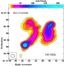
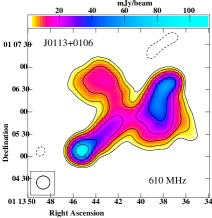
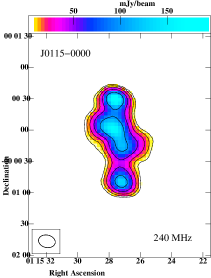
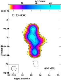
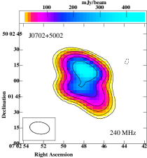
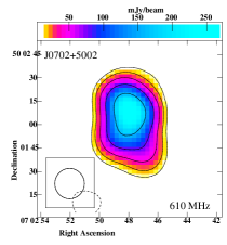
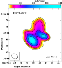
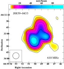
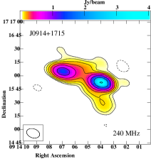
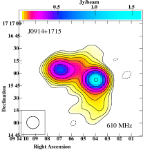
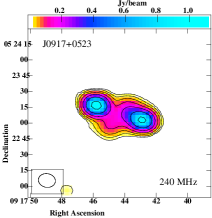
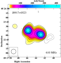
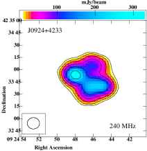
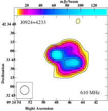
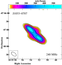
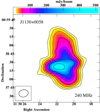
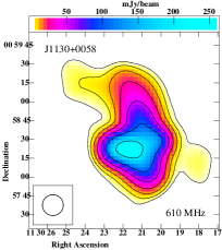
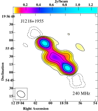
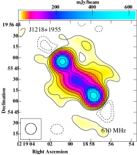
Figure 4.— The full synthesis GMRT images at 240 MHz (first and third columns)) and lower resolution versions of the 610 MHz data (second and fourth columns). Map parameters are summarized in Table 4.

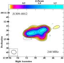
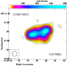
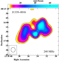
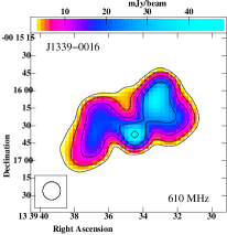
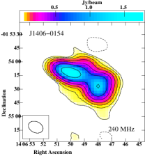
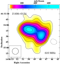
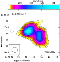
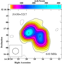
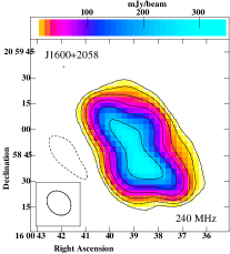
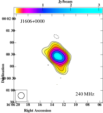
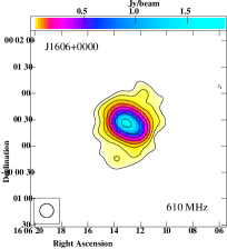
Figure 4.— continued.

References

- Albareti et al. (2017) Albareti, F. D., Allende Prieto, C., Almeida, A., et al. 2017, ApJS, 233, 25
- Becker et al. (1995) Becker, R. H., White, R. L., & Helfand, D. J. 1995, ApJ, 450, 559
- Begelman, Blandford & Rees (1980) Begelman, M. C., Blandford, R. D., & Rees, M. J. 1980, Nature, 287, 307
- Blundell & Rawlings (2000) Blundell, K. M., & Rawlings, S. 2000, AJ, 119, 1111
- Bridle & Greisen (1994) Bridle, A. H., Greisen E. W. 1994, The NRAO AIPS Project: a summary, AIPS Memo 87 (Charlottesville: NRAO)
- Capetti et al. (2002) Capetti, A., Zamfir, S., Rossi, P., Bodo, G., Zanni, C., & Massaglia, S. 2002, A&A, 394, 39
- Cheung (2007) Cheung, C. C. 2007, AJ, 133, 2097
- Cheung et al. (2009) Cheung, C. C., Healey, S. E., Landt, H., Verdoes Kleijn, G., & Jordán, A. 2009, ApJS, 181, 548
- Dennett-Thorpe et al. (2002) Dennett-Thorpe, J., Scheuer, P. A. G., Laing, R. A., et al. 2002, MNRAS, 330, 609
- Fanaroff & Riley (1974) Fanaroff, B. L., & Riley, J. M. 1974, MNRAS, 167, 31P
- Gillone, Capetti & Rossi (2016) Gillone, M., Capetti, A., & Rossi, P. 2016, A&A, 587, A25
- Gopal-Krishna et al. (2003) Gopal-Krishna, Biermann, P. L., & Wiita, P. J. 2003, ApJ, 594, L103
- Hao et al. (2010) Hao, J., McKay, T. A., Koester, B. P., et al. 2010, ApJS, 191, 254
- Hardcastle (2013) Hardcastle, M. J. 2013, MNRAS, 433, 3364
- Hodges-Kluck & Reynolds (2011) Hodges-Kluck, E. J., & Reynolds, C. S. 2011, ApJ, 733, 58
- Kharb et al. (2017) Kharb, P., Lal, D. V., & Merritt, D. 2017, Nature Astronomy, 1, 727
- Koss et al. (2012) Koss, M., Mushotzky, R., Treister, E., Veilleux, S., Vasudevan, R. & Trippe, M. 2012, ApJ, 746, L22
- Kraft et al. (2005) Kraft, R. P., Hardcastle, M. J., Worrall, D. M., & Murray, S. S. 2005, ApJ, 622, 149
- Lal & Rao (2005) Lal, D. V., & Rao, A. P. 2005, MNRAS, 356, 232
- Lal & Rao (2007) Lal, D. V., & Rao, A. P. 2007, MNRAS, 374, 1085
- Lal, Hardcastle & Kraft (2008) Lal, D. V., Hardcastle, M. J. & Kraft, R. P. 2008, MNRAS, 390, 1105
- Leahy & Parma (1992) Leahy, J. P., & Parma, P. 1992, Extragalactic Radio Sources. From Beams to Jets, 307
- Leahy & Williams (1984) Leahy, J. P., & Williams, A. G. 1984, MNRAS, 210, 929
- Liu et al. (2011) Liu, X., Shen, Y., Strauss, M. A. & Hao, L. 2011, ApJ, 737, 101
- Machalski et al. (2007) Machalski, J., Chyźy, K. T., Stawarz, L. & Koziel, D. 2007, A&A, 462, 43
- Merritt & Ekers (2002) Merritt, D., & Ekers, R. D. 2002, Science, 297, 1310
- Miley et al. (1972) Miley, G. K., Perola, G. C., van der Kruit, P. C. & van der Laan, H. 1972, Nature, 237, 269
- Mortlock, Webster & Francis (1999) Mortlock, D. J., Webster, R. L. & Francis, P. J. 1999, MNRAS, 309, 836
- Owen et al. (1985) Owen, F. N., O’Dea, C. P., Inoue, M. & Eilek, J. A. 1985, ApJ, 294, L85
- Palma et al. (2000) Palma, C., Bauer, F. E., Cotton, W. D., et al. 2000, AJ, 119, 2068
- Parma et al. (1985) Parma P., Ekers R. D. & Fanti R, 1985, A&AS, 59, 511
- Prasad & Chengalur (2012) Prasad, J., & Chengalur, J. 2012, Experimental Astronomy, 33, 157
- Roberts et al. (2015) Roberts, D. H., Cohen, J. P., Lu, J., Saripalli, L., & Subrahmanyan, R. 2015, ApJS, 220, 7
- Roberts et al. (2018) Roberts, D. H., Saripalli, L., Wang, K. X., et al. 2018, ApJ, 852, 47
- Rodriguez et al. (2006) Rodriguez, C., Taylor, G. B., Zavala, R. T., et al. 2006, ApJ, 646, 49
- Rossi et al. (2017) Rossi, P., Bodo, G., Capetti, A., & Massaglia, S. 2017, A&A, 606, A57
- Saripalli & Subrahmanyan (2009) Saripalli, L., & Subrahmanyan, R. 2009, ApJ, 695, 156
- Saripalli & Roberts (2018) Saripalli, L., & Roberts, D. H. 2018, ApJ, 852, 48
- Sudou, Iguchi & Murata (2003) Sudou H., Iguchi S. & Murata Y., 2003, Sci, 300, 1263
- Wang et al. (2003) Wang, T.-G., Zhou, H.-Y., & Dong, X.-B. 2003, AJ, 126, 113
- Worrall et al. (1995) Worrall, D. M., Birkinshaw, M., & Cameron, R. A. 1995, ApJ, 449, 93
- Zhang et al. (2007) Zhang, X.-G., Dultzin-Hacyan, D., & Wang, T.-G. 2007, MNRAS, 377, 1215