Simulations of Majorana spin flips in an antihydrogen trap

Abstract

The properties of antihydrogen ($\bar{\rm H}$) have, thus far, been probed at magnetic fields of $\sim 1$ T. It may be fruitful to perform some of these measurements at magnetic fields approaching 0 T. In this case, there could occur zeros in the magnitude of the $B$-field. The number and properties of the magnetic field zeros are investigated. For typical magnetic field geometries in $\bar{\rm H}$ traps, the zeros will occur as two groups of 5 closely spaced points instead of as a single point. Except in special cases, results from calculations show that these 10 zeros can be treated as independent sources of spin flip probability. Although the behavior of Majorana spin flip near higher order zeros should not be important in the $\bar{\rm H}$ traps, the probability for spin flip is calculated for the case of a quadratic zero. Finally, results are presented for a simple model of how magnetic field zeros would affect the trapped population of $\bar{\rm H}$.

I Introduction

More than 30 years ago, an effort was started to measure properties of the antihydrogen ($\bar{\rm H}$) atom with the goal of comparing them with their matter counterpartGabrielse et al. (1988). Because the properties of H and $\bar{\rm H}$ should be exactly the same by the CPT theorem, any difference would represent a fundamental discoveryBluhm et al. (1999). It is very difficult to generate any neutral antimatter atom or molecule beyond $\bar{\rm H}$ which means it is fortunate that so many properties of H are known to ultrahigh precision. In 2002, cold $\bar{\rm H}$ was experimentally formed at CERNAmoretti et al. (2002); Gabrielse et al. (2002). In 2010, the ALPHA collaboration trapped $\bar{\rm H}$Andresen et al. (2010) and within a yearAndresen et al. (2011a) demonstrated that the $\bar{\rm H}$ could be held for an extensive time, sufficient for precision measurements. To date, only the ALPHA collaboration has measured any property of the $\bar{\rm H}$ atom although several groups are attempting to measure various properties. Examples of precision measurements include the hyperfine splitting of the $1S$ statesAmole et al. (2012); Ahmadi et al. (2017a), the charge of the $\bar{\rm H}$Amole et al. (2014); Ahmadi et al. (2016), the energy difference between the $1S$ and $2S$ statesAhmadi et al. (2017b, 2018a), and the Lyman-$\alpha$ transitionAhmadi et al. (2018b). Extensions of these measurements could lead to accurate determination of other parameters. For example, a more accurate measurement of the Lyman-$\alpha$ transition would give the Lamb shift or the measurement of another narrow linewidth transition (e.g. 2S-4S) would allow the determination of the antiproton radius and the $\bar{\rm H}$ Rydberg constant.

The $\bar{\rm H}$ ground state has 4 non-degenerate levels in a magnetic field. By convention these are labeled $1Sa,1Sb,1Sc,1Sd$ from lowest to highest energy, see Fig. 1 of Ref. Amole et al. (2012). The $1Sa,1Sb$ states have decreasing energy with increasing $B$ and, thus, are high field seeking states which are expelled from a magnetic trap. The $1Sc,1Sd$ states have increasing energy with increasing $B$ and can be trapped. Above $\sim 0.1$ T, the states are effectively two pairs of states with a magnetic moment approximately that of a free electron giving a slope of $(dE/dB)/k_{B}\simeq\pm 2/3$ K/T. For small magnetic fields (less than $\sim 0.01$ T), the states are more accurately represented as hyperfine eigenstates with an $F=0$ state 1420 MHz below the $F=1$ states. For small $B$-field, the $F=1$ state is split to $M_{F}=1,0,-1$ in increasing order of energy. The $M_{F}=0,-1$ are the states that adiabatically connect to the trappable states.

Within the past few years, the ALPHA collaboration has successfully performed several high precision measurements as enumerated in the first paragraph. The trapping region is a tube of length $\sim 25$ cm and radius $\sim 2$ cm. We will denote motion along the axis to be axial motion represented by $z$ while the radial or angular motions will be represented by $x,y$. Measurements in this trap have taken place in magnetic fields of $\sim 1$ T which forces a comparison between the measured $\bar{\rm H}$ transition frequencies and calculated frequencies using the known properties of the positron and antiproton (e.g. masses, charges, and magnetic dipole moments). If the magnetic field were smaller, then some of the terms in the calculation of transition frequencies become irrelevant. As an example, the diamagnetic shift of the $1S-2S$ frequency would be less than 0.4 Hz for $B=1$ mTRasmussen et al. (2017). As another example, the shift in energy due to the motional Stark effect was estimated to be $\sim 300$ Hz in a 1 T fieldRasmussen et al. (2017) but would be much less than 1 Hz in a 1 mT field since the shift is proportional to $B^{2}$. This suggests that the path to, for example, $\sim 1-10$ Hz accuracy will be for the experiments to occur at smaller magnetic field.

One of the difficulties of working at a smaller $B$-field is that it might accidentally go to zero. In this case, the two trapped states, $M_{F}=0,-1$, could suffer a Majorana spin flip if the $\bar{\rm H}$ passes too close to a $B$-field zeroMajorana (1932); Zener (1932); Landau (1932). The Majorana spin flip occurs because the body frame direction of the $B$-field changes more rapidly than the precession frequency when passing near the zero. For $\bar{\rm H}$, the situation is somewhat complicated because the energies of the $F=1$ state are not exactly $-\mu BM_{F}$. However, for the size of $B$ where the spin flip is possible, the linear dependence of the energy on $B$ is good enough to obtain accurate spin flip cross sections. The main complicating factor for traps like that in the ALPHA device is that there is more than one zero and the zeros can be closely spaced, depending on the parameters, 5 zeros can be separated by less than 1 mm. This special condition warrants an investigation of the physics of spin-flip in this type of trap.

This paper is organized as follows. Section II gives the possible forms of the $B$-field near the zeros. Section III gives analytic expressions for the spin flip cross section and rate which are accurate when the zeros are separated. Section IV contains a comparison between the analytic approximation to the cross section and a fully numerical result; conditions are given for when the analytic approximation is accurate. Section V contains results for how the spin flip affects the energy distribution of trapped $\bar{\rm H}$s. There is a short conclusions section, Sec. VI. Section VIII is a short appendix that, for completeness, gives the derivation of the spin flip cross section for an isolated zero.

II Form of $\vec{B}$ near zeros

For the Majorana spin flip process, the velocity of the $\bar{\rm H}$ and the variation of the B-field near $|\vec{B}|=0$ determines the spin flip probability. Away from the zero, the $\bar{\rm H}$ magnetic moment adiabatically follows the magnetic field direction. To get a sense of the relevant scales, the precession of the positron spin is $\sim 30$ MHz at 1 mT. Since only $\bar{\rm H}$s with kinetic energy less than $\sim 1/2$ K are trapped, their speed is a few 10’s m/s. At 1 mT, the $\bar{\rm H}$ travels $\sim 1$ $\mu$m during one precession period. The spatial variation of the magnetic field near a zero is $\sim 1$ T/m. Taking the change in $B$ during one precession period to be $\sim 10\times$ smaller than $B$ suggests that only regions where the magnetic field is less than $\sim 0.1$ mT are important for spin flip.

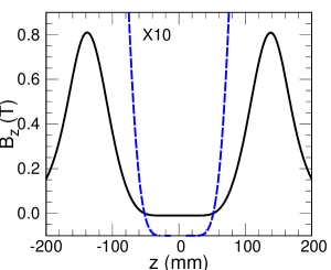
Figure 1: $B_{z}$ on the trap axis as a function of the axial position. $z=0$ corresponds to the trap center. This magnetic field is the superposition from 5 mirror coils. The dashed (blue) line is $10\times$ $B_{z}$.

To obtain an idea of how many and where the magnetic zeros appear, we numerically found the zeros for the magnetic field trap used in Refs. Ahmadi et al. (2017b, a, 2018a, 2018b) but shifted $B_{z}$ so that it was slightly negative, $B_{z}=-0.01$ T, in the central region instead of $\sim 1$ T. A schematic drawing of the trap is in any of these papers. Mirror coils provide the axial, $z$, confinement while octupole coils provide confinement in $x,y$. The radius of the trap is approximately 22 mm. The on axis $B_{z}$ is shown in Fig. 1 where the trapping region is between the $B_{z}$-maxima near $z=\pm 138$ mm. This magnetic field is mainly generated with 5 mirror coils. The outer two coils give a large positive $B_{z}$ on axis leading to the maxima. The middle 3 mirror coils have opposite current (bucked) to the outer coils giving a flattened B-field in the central region. This flattening is desirable because it increases the precision of the spectroscopic measurements and leads to a larger resonance region for the transitions whose frequencies are shifted by $B$. A nearly uniform $B$-field along $z$ sets the overall size of the on axis field. The octupole field is nearly zero on axis but plays a large role off axis.

The $10\times$ $B_{z}$ in Fig. 1 makes clearer the two axial positions where the $B$-field is near 0. There is a group of zeros near $z=-52$ mm and another near $z=52$ mm. Figure 2 shows the $x,y$ positions of the zeros near $z=-52$ mm. There is one zero nearly on axis and 4 that are at nearly the same radius and separated by 90^∘. The off axis zeros near $z=52$ mm are rotated by approximately 45^∘ from those shown in Fig. 2. Without the octupole field, there is only one zero and it is nearly on axis. The combination of the octupole field and the radial component of the magnetic field from the mirrors lead to the 4 off axis zeros.

Figure 2: Positions of the magnetic field zeros near $z=-52$ mm using the full model of the ALPHA trap. The central zero is actually $\simeq 16$ $\mu$m off the axis and is at a slightly shifted axial position ($z=-51.84$ mm) compared to the off axis zeros ($z=-51.96$ mm).

The form of the magnetic field near the possible zeros is described in this section for the case of an octupole field in $x,y$ plus a cylindrically symmetric field that varies in $x,y,z$. This geometry is important for the antihydrogen traps because both ALPHA and ATRAP have this magnetic field structure. For an idealization of either apparatus, there is an octupole magnetic field that increases with the radial distance from the center of the trap but whose magnitude has no dependence on the axial coordinate. There will also be a cylindrically symmetric magnetic field with a $z$-dependence on axis which is a low power, e.g. $z^{1}$. Two or more mirror coils can generate axially confining fields that are proportional to $z^{2}$ near the minimum or higher power (e.g. $z^{4}$ or $z^{6}$) when using 5 mirror coils as in ALPHA.

This idealization of the magnetic field is accurate away from the trap walls and in the region where the B-field is near its minimum value. The octupole field seriously deviates from the idealization only near the end of the octupole coils and near the walls ($r\simeq 22$ mm), but the zeros discussed below are always within the axial central half of the trap and far from the walls, see Fig. 2 and the caption. The B-fields from the mirrors only deviate from cylindrical symmetry due to the leads or manufacturing imperfections. Thus, the deviations from the ideal case should only lead to small linear terms near the zero which will only slightly modify the variation of the magnetic field. We compared our calculations of spin flip probability using the idealization to those using a full model of all of the ALPHA coils and found only negligible differences once the positions of the zeros were matched.

II.1 Octupole magnetic field

We will approximate the octupole field with the form

$$\vec{B}_{o}(x,y,z) = \frac{B_{w}}{r_{w}^{3}}(-x^{3}+3xy^{2},-y^{3}+3yx^{2},0)$$ (1)

$$= \frac{B_{w}r^{3}}{r_{w}^{3}}[-\hat{e}_{r}\cos(4\phi)+\hat{e}_{\phi}\sin(4\phi)]$$

where $r_{w}$ is the radius of the trap wall, $B_{w}$ is the magnitude of the octupole field at $r_{w}$, $r^{2}=x^{2}+y^{2}$, $\hat{e}_{r}=\hat{e}_{x}\cos(\phi)+\hat{e}_{y}\sin(\phi)$, and $\hat{e}_{\phi}=-\hat{e}_{x}\sin(\phi)+\hat{e}_{y}\cos(\phi)$. This octupole field has the property $|\vec{B}_{o}|=(r/r_{w})^{3}B_{w}$. The form of the octupole field in Eq. (1) will give zeros that are rotated from those shown in Fig. 2 but this rotation has no effect on the probability for a Majorana spin flip when averaged over all possible trajectories from trapped $\bar{\rm H}$s. We have chosen this form, instead of that rotated to match Fig. 2, to simplify the analysis below.

In all of the calculations below, we use $B_{w}/r_{w}^{3}=1.375\times 10^{5}$ T/m³ which is a typical value used in ALPHA experiments.

II.2 Octupole plus linear variation

The magnetic field which is cylindrically symmetric and has linear spatial dependence is

$$\vec{B}_{c} = \frac{B_{1}}{L}(x,y,-2(z-z_{0}))$$ (2)

$$= \frac{B_{1}}{L}[r\hat{e}_{r}-2(z-z_{0})\hat{e}_{z}]$$

where $-2B_{1}/L$ is the slope of $B_{z}$ on the axis at the zero which is at $(0,0,z_{0})$.

The zeros of the total magnetic field are the positions where all components of $\vec{B}_{o}+\vec{B}_{c}$ are zero. Since the octupole field has no $z$-component, all of the zeros are where $B_{c,z}=0$. This means all of the zeros have $z=z_{0}$. From the caption of Fig. 2, this is a good approximation to the actual $B$-field where the differences in the $z$-position of the zeros are less than $\simeq 0.1$ mm. The off axis zeros can be found by setting the coefficient of $\hat{e}_{\phi}$ and $\hat{e}_{r}$ separately equal to 0. Since the cylindrically symmetric field, $\vec{B}_{c}$, does not have a $\hat{e}_{\phi}$ component, this conditions sets the angles of the zeros from $\sin(4\phi_{0})=0$: $\phi_{0}=n\pi/4$ with $n=0,1,2,...,7$. Lastly, the coefficient of the $\hat{e}_{r}$ gives

$$-\frac{B_{w}}{r_{w}^{3}}\cos(4\phi_{0})r_{0}^{3}+\frac{B_{1}}{L}r_{0}=0$$ (3)

which can only be zero if $\cos(4\phi_{0})>0$ when $B_{1}/L>0$. This means only 4 of the angles allowed by the $\hat{e}_{\phi}$ condition give zeros for the $\hat{e}_{r}$ condition: $\phi_{0}=n\pi/2$ with $n=0,1,2,3$. If $B_{1}/L<0$, then the allowed angles are rotated by 45^∘ from the values for $B_{1}/L>0$. This feature matches that in the actual $B$-field. At each of these angles, the radius is the same value

$$r_{0}=\sqrt{\frac{B_{1}r_{w}^{3}}{B_{w}L}}.$$ (4)

These zeros have the same properties as those from the actual field: the off axis zeros have nearly the same radius and are separated by 90^∘. As described in Sec. II.1, the angles do not match Fig. 2 because of the choice of orientation of the octupole B-field (chosen for simplicity of the resulting analysis).

To give an idea of sizes, the off axis zeros in Fig. 2 are at $r_{0}\simeq 2.225\times 10^{-3}$ m. Using $B_{w}/r_{w}^{3}=1.375\times 10^{5}$ T/m³ from the previous section gives $B_{1}/L=0.681$ T/m.

For the Majorana spin flip, the variation of $\vec{B}$ in the neighborhood of a zero is important. The spatially linear variation $(x,y,z)=(x_{0}+\delta x,y_{0}+\delta y,z_{0}+\delta z)$ has the form

$$\vec{B}=\frac{B_{1}}{L}(\delta x,\delta y,-2\delta z)+O(\delta^{3})$$ (5)

for the on axis zero where $O(\delta^{3})$ indicates the correction is cubic in the position change. For the off axis zero at $\phi_{0}=0$ (i.e. on the $x$-axis), a Taylor series expansion gives

$$\vec{B}=-\frac{2B_{1}}{L}(\delta x,-2\delta y,\delta z)+O(\delta^{2})$$ (6)

which has the same form as for the central zero except with a rotated coordinate system and double the slope. All of the off axis zeros have these properties: same form, double the slope of the central zero, and rotated coordinate system.

An important question is whether the zeros will give independent spin flip probabilities for most trajectories or whether the nearness of other zeros will affect the spin flip process. As will be shown in Sec. IV, the zeros give independent contributions to the cross section as long as the separation is larger than (approximately) the square root of the spin flip cross section. This situation always occurs at large $B_{1}/L$ since the separation increases with increasing $B_{1}/L$ while the cross section decreases. The simulations show where this approximation gives good results and where it is poor.

II.3 Octupole plus quadratic variation

The magnetic field which is cylindrically symmetric and has quadratic spatial dependence is

$$\vec{B}_{c} = (0,0,B_{0})+\frac{B_{2}}{L^{2}}(-xz,-yz,z^{2}-\frac{1}{2}r^{2})$$ (7)

$$= \left(B_{0}+\frac{B_{2}}{L^{2}}[z^{2}-\frac{1}{2}r^{2}]\right)\hat{e}_{z}-\frac{B_{2}}{L^{2}}rz\hat{e}_{r}$$

where the on axis minimum of $B_{z}$ is $B_{0}$ at $z=0$ and $B_{2}/L^{2}$ is half the curvature of the B-field on axis. When only the outer coils make the magnetic trap, the $B_{2}/L^{2}\sim 15$ T/m². When the field is flattened as in Fig. 1, there can be inadvertent minima when attempting to obtain a flattened $B$-field with $B_{2}/L^{2}\sim 1$ T/m² or somewhat smaller.

There can only be zeros on axis if $B_{0}<0$ and they are at $z_{0}=\pm\sqrt{-B_{0}L^{2}/B_{2}}$ and $r_{0}=0$. The off axis case is a bit more complicated. The $\hat{e}_{\phi}$ condition still gives $\sin(4\phi_{0})=0$: $\phi_{0}=n\pi/4$ with $n=0,1,2,...,7$. The $\hat{e}_{r}$ condition gives

$$-\frac{B_{2}}{L^{2}}r_{0}z_{0}-\frac{B_{w}}{r_{w}^{3}}r_{0}^{3}\cos(4\phi_{0})=0$$ (8)

which restricts $\phi_{0}=n\pi/2$ with $n=0,1,2,3$ if $z_{0}<0$ and $\phi_{0}=n\pi/4$ with $n=1,3,5,7$ if $z_{0}>0$. These relations explain why the off axis zeros were rotated by 45^∘ in the actual magnetic field associated with Fig. 1. This also gives the relationship $r^{2}_{0}={\cal L}|z_{0}|$ with ${\cal L}=(r_{w}^{3}/B_{w})(B_{2}/L^{2})$. The condition from $\hat{e}_{z}$ gives

$$z^{2}_{0}-\frac{1}{2}{\cal L}|z_{0}|-z^{2}_{0,a}=0$$ (9)

where $z^{2}_{0,a}=-B_{0}L^{2}/B_{2}$ is from the on axis zero. There is a small range of cases where there are zeros with positive $B_{0}$ but it is less than $\sim 10^{-8}$ T and, therefore, experimentally irrelevant. For $B_{0}\leq 0$,

$$|z_{0}|=\frac{\cal L}{4}+\sqrt{({\cal L}/4)^{2}+z^{2}_{0,a}}\quad{\rm and}\quad r_{0}=\sqrt{{\cal L}|z_{0}|}$$ (10)

where $z^{2}_{0,a}\geq 0$.

It is worth considering the sizes of various terms using $B_{2}/L^{2}\sim 10$ T/m² and $B_{w}/r_{w}^{3}\sim 10^{5}$ T/m³. The case $B_{0}=0$ is simple giving $|z_{0}|=(B_{2}/L^{2})/(2B_{w}/r_{w}^{3})$ and $r_{0}=|z_{0}|/\sqrt{2}$. This gives a $z$-separation of $\sim 0.1$ mm and a similar size for $r_{0}$ implying that $B_{0}=0$ might lead to interesting results. However, even relatively small $B_{0}$ leads to the approximation in Sec. II.2 working well. For example, $B_{0}=-1$ mT and $B_{2}/L^{2}=10$ T/m² gives a separation in z of $20$ mm while changing to $B_{0}=0.1$ mT gives a separation of 6.3 mm. Therefore, only the $B_{0}=0$ case is probably of interest.

II.4 Octupole plus quartic variation

For the flatter potentials (like that pictured in Fig. 1), the zeros become like the case of well separated linear zeros, Sec. II.2. For example, in Fig. 1, the zeros for the case $B_{z}(0,0,0)=-10$ mT gave a separation of $\sim 104$ mm while $-1$ mT gave a separation of $\sim 80$ mm. It is likely that imperfections in the magnetic field will mean this case will never be experimentally interesting.

III Flip cross section and rate: linear zero approximation

As a baseline, the Majorana spin flip probability will be calculated for a single zero. Since all of the zeros, Eqs. (5,6), have a linear approximation of the form Eq. (2) (except rotated), we only discuss the spin flip for that case. The time dependent magnetic field at the atom is determined by the motion of the atom which is assumed to be a straight line at constant speed. To simplify the analysis, the origin of the coordinate system is at the zero of the magnetic field. The position of the $\bar{\rm H}$ is given by

$$\vec{r}(t)=\vec{b}+\vec{v}t$$ (11)

where $b$ is the impact parameter, $v$ is the speed, and we define the time of closest approach as $t=0$ which means $\vec{b}\cdot\vec{v}=0$. Since the position linearly depends on time and the magnetic field linearly depends on the position, the magnetic field linearly depends on time. For this case, Landau-Zener type theories can be used to analytically obtain the transition probability between different statesSinitsyn et al. (2017). From the probability as a function of $\vec{b}$ and $\vec{v}$, cross sections for particular transitions have been obtained beforeZener (1932); Landau (1932); Sinitsyn et al. (2017). For completeness, the derivation of the flip probability is given in the appendix, Sec. VIII.

For $\bar{\rm H}$, the upper two energy levels of the $F=1$ state are the only ones that are trapped in the magnetic field. The upper level is $M_{F}=-1$ and the next level is $M_{F}=0$. The cross section for various flip processes is calculated from the transition probability which is a function of $\vec{b}$ and $\vec{v}$ for a given $\bar{\rm H}$ speed, $v$. The derivation of the cross section for one linear zero is given in the appendix, Sec. VIII,

$$\sigma_{1\leftarrow-1} = \sigma(v)\qquad{\rm and}\qquad\sigma_{0\leftarrow-1}=2\sigma(v)$$

$$\sigma_{-1\leftarrow 0} = 2\sigma(v)\qquad{\rm and}\qquad\sigma_{1\leftarrow 0}=2\sigma(v)$$ (12)

where $\sigma(v)=\hbar v/(\mu B_{1}/L)$ with $\mu=9.28\times 10^{-24}$ J/T $\simeq k_{B}2/3$ K/T, the magnetic moment of the positron. This is an interesting result in that the flip rate, $v\sigma$, is proportional to the kinetic energy of the $\bar{\rm H}$. Thus, the atoms that are lost will tend to be the hottest.

For the case of the octupole plus linear variation in $z$, there were 5 zeros. The 4 off axis zeros had twice the slope as on the central axis. If all 5 zeros give an independent contribution to the Majorana flip cross section, the total cross section for the group of 5 will be

$$\sigma_{1\leftarrow-1} = 3\sigma(v)\qquad{\rm and}\qquad\sigma_{0\leftarrow-1}=6\sigma(v)$$

$$\sigma_{-1\leftarrow 0} = 6\sigma(v)\qquad{\rm and}\qquad\sigma_{1\leftarrow 0}=6\sigma(v)$$ (13)

where $\sigma(v)=\hbar v/(\mu B_{1}/L)$. For the actual traps, there are two groups of 5 zeros implying the total flip cross sections are double these results.

IV Comparison to numerical

In this section, the spin flip cross section from the numerical solution of the time dependent Schrödinger equation is presented.

The time dependent Schrödinger equation was solved using the Crank-Nicolson methodCrank and Nicolson (1996):

$$\vec{\psi}(t+\delta t)=\frac{1-iH\delta t/(2\hbar)}{1+iH\delta t/(2\hbar)}\vec{\psi}(t)$$ (14)

where the Hamiltonian, $H$ in Eq. (23), is evaluated at time $t+\delta t/2$. For spin-1, the Hamiltonian is a $3\times 3$ matrix so the solution of this matrix equation is relatively fast.

The somewhat tricky aspect of obtaining the cross section is to determine the fraction of population where $M_{F}$ has changed. The eigenstates when $\vec{B}=B(\sin\theta\cos\phi,\sin\theta\sin\phi,\cos\theta)$ are

$$\vec{\psi}_{\pm 1}=\begin{pmatrix}\frac{1}{2}(1\pm\cos\theta)e^{-i\phi}\\ \frac{1}{\sqrt{2}}\sin\theta\\ \frac{1}{2}(1\mp\cos\theta)e^{i\phi}\end{pmatrix}\quad\vec{\psi}_{0}=\begin{pmatrix}-\frac{1}{\sqrt{2}}\sin\theta e^{-i\phi}\\ \cos\theta\\ \frac{1}{\sqrt{2}}\sin\theta e^{i\phi}\end{pmatrix}$$ (15)

When solving the time dependent Schrödinger equation, the magnetic field will start out in one direction and finish in another. We used these equations to start the wave function at the initial time and to project onto the final states. In the calculations, we started the time propagation so that the $\bar{\rm H}$ is far enough from the zeros that initially the state adiabatically follows the changing direction of $\vec{B}$ and stopped the propagation when this condition was again satisfied.

We found that using Eq. (11) did not give results that converged well with the starting and final time. The problem is that starting with Eq. (11) does not adequately account for the slight difference between the adiabatic and actual wave function unless the magnetic field is very large. This causes the calculations to be quite slow because then the wave function needs to be propagated for longer times and the time steps need to be smaller to account for the larger energy splittings. We found that a $\vec{r}(t)$ where the velocity smoothly turned on from 0 to $\vec{v}$ and then smoothly turned back to 0 allowed for accurate calculation of spin flip probabilities with relatively little numerical effort. We used

$$\frac{d\vec{v}_{t}(t)}{dt}=\frac{\vec{v}}{\tau\sqrt{\pi}}\left[e^{-(t-t_{i})^{2}/\tau^{2}}-e^{-(t-t_{f})^{2}/\tau^{2}}\right]$$ (16)

where $\tau$ is the duration of the turn-on and $d\vec{r}(t)/dt=\vec{v}_{t}(t)$ for the time dependent position. We then solved the time dependent Schrödinger equation from $t_{i}-6\tau$ to $t_{f}+6\tau$. As long as $\tau$ was much larger than $\hbar/(\mu B)$ with $B$ evaluated at the starting and final time, then the convergence was much faster with respect to $t_{i},t_{f}$.

For the calculation of the cross section, we used a Monte Carlo sampling of the $\hat{v}$ and $\vec{b}$. The random parameters were chosen as: $b^{2}$ randomly chosen with a flat distribution between 0 and $b^{2}_{max}$, $\hat{v}$ randomly chosen with a flat distribution on the surface of a unit sphere, and $\hat{b}$ randomly chosen from a flat distribution on the great circle defined by $\hat{v}\cdot\hat{b}=0$. The cross section for a transition is the average probability for that transition times $\pi b^{2}_{max}$. We checked for convergence with respect to $b_{max}$ and the number of trajectories. The $b_{max}$ can be estimated from Eq. (24) by setting $\Gamma>16/\pi$ for all angles and adding this to the $r_{0}$ of the off-axis zeros.

As a test of the program, we solved for the spin flip cross section for the pure linear $B$-field, Eq. (2). We found that the cross section only differed from the analytic value, Eq. (III), due to statistical sampling.

IV.1 Octupole plus linear variation

In this section are the numerical results for the case of the octupole plus linearly varying $\vec{B}_{c}$ described in Sec. II.2. For this case, we compared the cross section for independent contribution from the 5 zeros, Eq. (III), to that from a numerical calculation. In the numerical calculation, we ran approximately 200,000 trajectories to obtain adequate statistics for the Monte Carlo cross section.

The case shown in Figs. 1 and 2 has a linear parameter $B_{1}/L=0.681$ T/m. Using these parameters and $v=50$ m/s, we found the Monte Carlo result to be the same as Eq. (III) within the statistical uncertainty. For this case, $\sigma(v)=8.33\times 10^{-10}$ m².

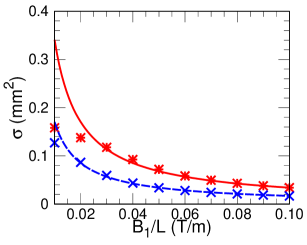
Figure 3: The numerically calculated flip cross sections, $|\Delta M_{F}|=1$ (red $*$) and $|\Delta M_{F}|=2$ (blue $\times$), compared to the separated zero approximation, Eq. (III), solid red line and blue dashed line. The statistical uncertainty is less than the size of the symbols.

To understand when to expect the separated zero approximation, Eq. (III), to fail, we plot the numerically calculated cross sections versus $B_{1}/L$ in Fig. 3. As in the approximation in Eq. (III), we found that the cross sections for $|\Delta M_{F}|=1$ were all the same and those for $|\Delta M_{F}|=2$ were all the same. We also show the results for the separated zero approximation, Eq. (III), as a comparison. As can be seen, there starts to be noticeable differences when $B_{1}/L<0.03$ for the $|\Delta M_{F}|=1$ case. At the lowest $B_{1}/L$ calculated (0.01 T/m), the numerical result is more than a factor of 2 smaller than the separated zero approximation. The $|\Delta M_{F}|=2$ is better matched by the approximation with substantial difference only for the smallest $B_{1}/L$. It seems reasonable that the separated zero approximation will break down when the flip cross section equals $\pi r_{0}^{2}$ where the $r_{0}$ is the radius of the off axis zeros, Eq. (4). For the parameters in this section, this condition gives $B_{1}/L\sim 0.022$ T/m for the $|\Delta M_{F}|=1$ case and $B_{1}/L\sim 0.015$ T/m for the $|\Delta M_{F}|=2$ case. These values are reasonably close to where the differences begin to appear in Fig. 3. For the $|\Delta M_{F}|=1$ case, this condition is $B_{1}/L=\sqrt{6\hbar vB_{w}/(\mu r_{w}^{3})}$ and is $\sqrt{2}$ smaller for the $|\Delta M_{F}|=2$ case. Experimental control of magnetic fields at this level is possibleAhmadi et al. (2017a, 2018a).

IV.2 Octupole plus quadratic variation

For this section, we will consider the cases where 1 T/m${}^{2}\leq B_{2}/L^{2}\leq 10$ T/m² which is a reasonable range for the $\bar{\rm H}$ traps. The case of an octupole field plus quadratic cylindrical field, Eq. (7), has 3 situations worth considering for these parameters: $B_{0}>0.025$ mT, $B_{0}=0$ T, and $B_{0}<-0.05$ mT.

The case $B_{0}>0.025$ mT is the simplest. The cross section is, within numerical errors, consistent with 0. The spin can adiabatically follow the changing direction of $\vec{B}$ for this case. We did not test how small can $B_{0}$ be before the cross section is non-negligible since $0.025$ mT is already below the accuracy for the experimental values of trap parameters.

The next simplest case is $B_{0}<-0.05$ mT. In this situation, there are two groups of 5 zeros near $|z_{0}|\simeq\sqrt{-B_{0}L^{2}/B_{2}}>1.6$ mm. In this case, the $B$-field in the neighborhood of the zeros is approximately that of the linear variation case with $B_{1}/L\simeq z_{0,a}B_{2}/L^{2}=\sqrt{-B_{0}B_{2}/L^{2}}$. In this limit of $B_{0}$, the zeros are relatively separated so the approximation in Eq. (III) can be used. For this case, the 10 zeros sum to give cross sections

$$\sigma_{1\leftarrow-1} = 6\sigma(v)\qquad{\rm and}\qquad\sigma_{0\leftarrow-1}=12\sigma(v)$$

$$\sigma_{-1\leftarrow 0} = 12\sigma(v)\qquad{\rm and}\qquad\sigma_{1\leftarrow 0}=12\sigma(v)$$ (17)

where $\sigma(v)=\hbar v/(\mu\sqrt{-B_{0}B_{2}/L^{2}})$. The numerical results are compared to this approximation in Fig. 4. As with the comparison in Fig. 3 for the linear zero, the agreement between the separated zero approximation and the numerical result is good until the separation of the zeros is comparable to the square root of the cross section.

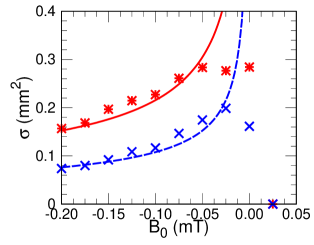
Figure 4: The numerically calculated flip cross sections, $|\Delta M_{F}|=1$ (red $*$) and $|\Delta M_{F}|=2$ (blue $\times$), compared to the separated zero approximation, Eq. (IV.2), solid red line and blue dashed line. The statistical uncertainty is less than the size of the symbols

The last important range is $B_{0}\sim 0$. For this value of $B_{0}$, the cross section is finite instead of diverging as in Eq. (IV.2). The approximate size is that for the independent zeros where the square root of the cross section is comparable to the separation of the zeros as with the case in Fig. 3.

V Antihydrogen loss model

This section contains results for a simple model calculation for the loss of $\bar{\rm H}$s from a trap for the conditions of Figs. 1 and 2. For this case there are 10 well separated zeros and the cross section for the various flip processes are twice the values in Eq. (III) with $B_{1}/L=0.681$ T/m.

In the ALPHA experiment, the volume of the trap is $\sim 100$ cm³ and they have demonstrated trapping of $\sim 100$ atomsAhmadi et al. (2017c, 2018a, 2018b). Thus, for absolute numbers we will take the $\bar{\rm H}$ density to be 1 cm^-3. Because the trap depth is only $\sim\frac{1}{2}k_{B}$K and the $\bar{\rm H}$s are formed at much higher temperatures, the distribution of atoms is approximately a flat distribution in velocity space within a sphere corresponding to a kinetic energy of $\simeq\frac{1}{2}k_{B}$K leading to a normalized distribution with respect to speed of $P(v)=3v^{2}/v_{\rm max}^{3}$. This distribution gives good agreement with measurementsAndresen et al. (2011b); Ahmadi et al. (2018b). From these parameters, we can estimate the rate for a spin flip process with cross section $\sigma=C\sigma(v)$ with $\sigma(v)=\hbar v/(\mu B_{1}/L)$ to be

$$\Gamma=\rho\frac{3}{v^{3}_{\rm max}}\int_{0}^{v_{\rm max}}Cv\sigma(v)v^{2}dv=\frac{3}{5}\rho v_{\rm max}C\sigma(v_{\rm max})$$ (18)

where $\rho$ is the number density of $\bar{\rm H}$s and $v_{\rm max}\simeq 91$ m/s for $KE_{max}=\frac{1}{2}k_{B}$K. Using these numbers, the $|\Delta M_{F}|=2$ rate (uses $C=6$) is $\Gamma\simeq 0.83$ s^-1 and the $|\Delta M_{F}|=1$ rate (uses $C=12$) is twice this value. In the ALPHA experiment, the two trapped states are formed with equal probability so the loss rate is the average of these, $\Gamma\simeq 1.2$ s^-1. This suggests that the zeros can not be present for more than a couple 10’s of seconds before a substantial fraction of the $\bar{\rm H}$s are lost.

An important question is how the populations evolve if the zeros are present for a substantial amount of time. This is not completely trivial because the higher energy $\bar{\rm H}$s are preferentially lost and because the zeros mix the two trapped states as well as leading to loss. We solved the coupled rate equations at each velocity for the flat velocity distribution described above with $E_{\rm max}=\frac{1}{2}k_{B}$K. The $\bar{\rm H}$s were started with a flat distribution in velocity and equal probability in the $M_{F}=0$ and $-1$ states: the energy distributions are ${P}_{-1}(E)={P}_{0}(E)=(3/4)E^{1/2}/E_{\rm max}^{3/2}$. We then evolved the distributions using twice the rates from Eq. (III) with $B_{1}/L=0.681$ T/m. The results are shown in Fig. 5 for the initial distribution and when 10% and when 30% of the $\bar{\rm H}$s have been lost. As can be seen, the higher energy $\bar{\rm H}$s are preferentially lost. Also, the distribution goes from equal population in $M_{F}=0$ and $-1$ to a larger fraction of $M_{F}=-1$. This is because the loss rate from $M_{F}=0$ is larger.

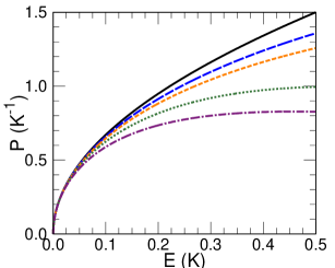
Figure 5: The energy distribution of $\bar{\rm H}$s after different amounts of interaction with $B$-field zeros. Both the $M_{F}=0$ and $-1$ states start with the distribution given by the black solid line. At the time when 10% of the $\bar{\rm H}$s have been lost, the $M_{F}=-1$ distribution is the dashed (blue) line and the $M_{F}=0$ distribution is the short dashed (orange) line. At the time when 30% of the $\bar{\rm H}$s have been lost, the $M_{F}=-1$ distribution is the dotted (green) line and the $M_{F}=0$ distribution is the dot-dashed (purple) line.

There are two major limitations of the model. The first is that the higher energy $\bar{\rm H}$s are in, effectively, a spatially larger trap. Although the trapping potential in Refs. Ahmadi et al. (2017b, a, 2018a, 2018b) are relatively flat, it is not an infinite square well. This means that the higher energy $\bar{\rm H}$s will pass by the zeros less often than in the simple model calculation. The second is that the mixing between the different degrees of freedom takes some time which can lead to depletion of certain types of trajectories. Again, this will lead to a somewhat smaller loss rate for the regions of phase space that does not mix quickly. Reference Zhong et al. (2018) found that the higher energy trajectories tended to mix more quickly which might somewhat counteract the effect of the somewhat larger trap volume at higher energy.

VI Conclusions

A description was given of the type of $B$-field zeros expected in $\bar{\rm H}$ traps. The octupole magnetic field that gives trapping in the radial direction leads to the case where the zeros will typically be in two groups of 5 zeros with the two groups having a large axial separation. The spacing of the zeros within a group of 5 is proportional to the square root of the slope of the $B$-field on axis and inversely proportional to the octupole strength. The cross section for the Majorana spin flip is proportional to the speed of the $\bar{\rm H}$ and inversely proportional to the slope of the magnetic field on axis at the $B$-field zero. Interestingly, for typical octupole trapping fields, the cross section is independent of the octupole field strength. Numerical calculation of the spin flip cross section were performed and were compared to analytic expressions for the spin flip cross section. The analytic cross sections are accurate as long as the square of the separation of the zeros is larger than the spin flip cross sections.

The evolution of the trap population was calculated for a simple model. In this model, the $\bar{\rm H}$s have a flat velocity distribution up to a maximum energy; this maximum energy is the trap depth. This simple model showed that the higher energy $\bar{\rm H}$s are preferentially lost and that an equal distribution of $M_{F}=-1$ and $0$ states becomes somewhat biased to $M_{F}=-1$.

The results presented above may be useful in designing a strategy for performing experiments on $\bar{\rm H}$ with small $B$-fields. For example, since the loss rate for an individual $\bar{\rm H}$ for typical parameters is $\sim 10^{-2}$ s^-1 and that the loss rate is highest just after the appearance of the zeros, an experiment might slowly lower the uniform $B$-field until the Majorana spin flips start occurring. At that point, the $B$-field can be increased to the point that the flips stop. As long as this manipulation occurs on a time scale less than a couple 10’s of seconds, there will not be a substantial loss of $\bar{\rm H}$s. Finally, it is possible to use these zeros to diagnose properties of the magnetic field that might be useful in experiments. For example, in a measurement of the effect of gravity on $\bar{\rm H}$s, it is important to not have a spatial gradient in the vertical direction which can mimic the force from gravity. By comparing the expected and measured positions where the spin flips occur, the size of a spatial gradient in the vertical direction can be diagnosed.

VII Acknowledgment

MAA was supported by the Purdue University SURF program, CJR was supported by the National Science Foundation under Award No. 1460899-PHY REU program, and FR was supported by the National Science Foundation under Award No. 1806380-PHY.

VIII Appendix

This section gives the derivation of the spin flip cross section for completeness.

Start with the form for the magnetic field, Eq. (2) with $z_{0}=0$, and the position as a function of time, Eq. (11). Define the magnitudes $v,b$ and the angles $\alpha,\beta$ where

$$\vec{v} = v(\sin(\beta),0,\cos(\beta))$$

$$\vec{b} = b(\cos(\alpha)\cos(\beta),\sin(\alpha),-\cos(\alpha)\sin(\beta)).$$ (19)

In this equation, advantage has been taken of the cylindrical symmetry of the magnetic field to define the velocity vector to be in the $xz$ plane. The time dependent magnetic field is then

$$\vec{B}(t) = \frac{B_{1}b}{L}(\cos(\alpha)\cos(\beta),\sin(\alpha),2\cos(\alpha)\sin(\beta))$$ (20)

$$+\frac{B_{1}v}{L}(\sin(\beta),0,-2\cos(\beta))t.$$

The coordinate system is now rotated so that the term multiplying $t$ is purely in the $z$-direction and the constant part of $B_{z}$ is removed by defining $t=0$ as the time of smallest $|\vec{B}|$:

$$\vec{B}(t) = \frac{B_{1}b}{L}(\frac{2\cos(\alpha)}{\sqrt{1+3\cos^{2}(\beta)}},\sin(\alpha),0)$$ (21)

$$+\frac{B_{1}v}{L}\sqrt{1+3\cos^{2}(\beta)}(0,0,1)t.$$

Lastly, rotate in the $xy$ plane so that $B_{y}=0$ to find

$$\vec{B}(t) = \hat{e}_{x}\frac{B_{1}b}{L}\sqrt{\frac{4\cos^{2}(\alpha)}{1+3\cos^{2}(\beta)}+\sin^{2}(\alpha)}$$ (22)

$$+\hat{e}_{z}\frac{B_{1}v}{L}\sqrt{1+3\cos^{2}(\beta)}t$$

$$\equiv (B_{x},0,\dot{B}_{z}t)$$

which defines the size of the transverse magnetic field and the size of the time derivative of the magnetic field along $z$. The Hamiltonian for the spin system is defined as

$$H=-\frac{\mu}{s\hbar}\vec{B}(t)\cdot\vec{S}$$ (23)

where $s=1$ for the $F=1$ case and would be $s=1/2$ for a spin-1/2 system.

We will first treat the more familiar spin-1/2 system because there is only one spin flip possibility. Using Landau-Zener formalism,Majorana (1932); Zener (1932); Landau (1932); Sinitsyn et al. (2017) the spin flip probability for a spin-1/2 system would be

$$P_{-1/2\leftarrow 1/2}=e^{-2\pi\Gamma}\quad{\rm with}\quad\Gamma=\frac{\mu B_{x}^{2}}{2\hbar\dot{B}_{z}}.$$ (24)

To obtain the cross section for the spin flip, the probability needs to be averaged over $\cos(\beta)$ and $\alpha$ and integrated over $2\pi bdb$:

$$\sigma(v)=\frac{2\pi}{4\pi}\int_{0}^{\infty}\int_{-1}^{1}\int_{0}^{2\pi}P_{-1/2\leftarrow 1/2}d\alpha d(\cos\beta)bdb$$ (25)

Perform the integration with respect to $bdb$ first to obtain

$$\sigma(v)=\frac{vL\hbar}{4\pi\mu B_{1}}\int_{-1}^{1}\int_{0}^{2\pi}\frac{(1+3s^{2})^{3/2}}{4-3(1-s^{2})\sin^{2}(\alpha)}d\alpha ds$$ (26)

where the transformation of variables $s=\cos\beta$ was used. Integrating over $\alpha$ gives

$$\sigma(v)=\frac{vL\hbar}{4\pi\mu B_{1}}\int_{-1}^{1}\pi(1+3s^{2})ds=\frac{\hbar v}{\mu B_{1}/L}$$ (27)

The case for spin 1 can be done analytically using a result from Ref. Sinitsyn et al. (2017). The parameters for the Majorana spin flip can be converted to their parameters:

$$b_{1} = -b_{3}=-\frac{\mu B_{1}v}{L\hbar}\sqrt{1+3\cos^{2}\beta}$$

$$g_{1} = g_{2}=-\frac{\mu Bb}{L\hbar\sqrt{2}}\left(\frac{\cos^{2}\alpha}{1+3\cos^{2}\beta}+\sin^{2}\alpha\right)^{1/2}$$ (28)

and $b_{2}=0$. This leads to probabilities of the same form as for the spin 1/2 system so that after integrating over impact parameter and averaging over $\alpha,\cos\beta$, the cross sections have the same form:

$$\sigma_{1\leftarrow-1} = \sigma(v)\qquad{\rm and}\qquad\sigma_{0\leftarrow-1}=2\sigma(v)$$

$$\sigma_{-1\leftarrow 0} = 2\sigma(v)\qquad{\rm and}\qquad\sigma_{1\leftarrow 0}=2\sigma(v)$$ (29)

where we have only included transitions out of the trapped $M_{F}=0,-1$ states.

References

- Gabrielse et al. (1988) G. Gabrielse, S. L. Rolston, L. Haarsma, and W. Kells, “Antihydrogen production using trapped plasmas,” Phys. Lett. A 129, 38 (1988).
- Bluhm et al. (1999) R. Bluhm, V. A. Kosteleckỳ, and N. Russell, “CPT and Lorentz tests in hydrogen and antihydrogen,” Phys. Rev. Lett. 82, 2254 (1999).
- Amoretti et al. (2002) M. E. A. Amoretti et al., “Production and detection of cold antihydrogen atoms,” Nature 419, 456 (2002).
- Gabrielse et al. (2002) G. Gabrielse et al., “Background-free observation of cold antihydrogen with field-ionization analysis of its states,” Phys. Rev. Lett. 89, 213401 (2002).
- Andresen et al. (2010) G. B. Andresen et al., “Trapped antihydrogen,” Nature 468, 673 (2010).
- Andresen et al. (2011a) G. B. Andresen et al., “Confinement of antihydrogen for 1,000 seconds,” Nat. Phys. 7, 558 (2011a).
- Amole et al. (2012) C. Amole et al., “Resonant quantum transitions in trapped antihydrogen atoms,” Nature 483, 439 (2012).
- Ahmadi et al. (2017a) M. Ahmadi et al., “Observation of the hyperfine spectrum of antihydrogen,” Nature 548, 66 (2017a).
- Amole et al. (2014) C. Amole et al., “An experimental limit on the charge of antihydrogen,” Nat. Commun. 5, 3955 (2014).
- Ahmadi et al. (2016) M. Ahmadi et al., “An improved limit on the charge of antihydrogen from stochastic acceleration,” Nature 529, 373 (2016).
- Ahmadi et al. (2017b) M. Ahmadi et al., “Observation of the 1S–2S transition in trapped antihydrogen,” Nature 541, 506 (2017b).
- Ahmadi et al. (2018a) M. Ahmadi et al., “Characterization of the 1S–2S transition in antihydrogen,” Nature 557, 71 (2018a).
- Ahmadi et al. (2018b) M. Ahmadi et al., “Observation of the 1S–2P Lyman- transition in antihydrogen,” Nature 561, 211 (2018b).
- Rasmussen et al. (2017) C. O. Rasmussen, N. Madsen, and F. Robicheaux, “Aspects of 1S–2S spectroscopy of trapped antihydrogen atoms,” J. Phys. B 50, 184002 (2017).
- Majorana (1932) E. Majorana, “Atomi orientati in campo magnetico variabile,” Il Nuovo Cimento 9, 43 (1932).
- Zener (1932) C. Zener, “Non-adiabatic crossing of energy levels,” Proc. R. Soc. Lond. A Math. Phys. Sci. 137, 696 (1932).
- Landau (1932) L. D. Landau, “Zur theorie der energieubertragung ii,” Z. Sowjetunion 2, 46 (1932).
- Sinitsyn et al. (2017) N. A. Sinitsyn, J. Lin, and V. Y. Chernyak, “Constraints on scattering amplitudes in multistate Landau-Zener theory,” Phys. Rev. A 95, 012140 (2017).
- Crank and Nicolson (1996) J. Crank and P. Nicolson, “A practical method for numerical evaluation of solutions of partial differential equations of the heat-conduction type,” Adv. Comput. Math. 6, 207 (1996).
- Ahmadi et al. (2017c) M. Ahmadi et al., “Antihydrogen accumulation for fundamental symmetry tests,” Nat. Commun. 8, 681 (2017c).
- Andresen et al. (2011b) G. B. Andresen et al., “Confinement of antihydrogen for 1,000 seconds,” Nat. Phys. 7, 558 (2011b).
- Zhong et al. (2018) M. Zhong, J. Fajans, and A. F. Zukor, “Axial to transverse energy mixing dynamics in octupole-based magnetostatic antihydrogen traps,” New J. Phys. 20, 053003 (2018).