Multimaterial Heat Flow Verification

Abstract

Multimaterial heat diffusion can be a challenging numerical problem when the material boundaries are misaligned with the numerical grid. Even when the boundaries start out aligned, they typically become misaligned through hydrodynamic motion. There are usually a number of methods for handling multimaterial cells in any given hydro code. One of the simplest methods is to replace the multimaterial cell by an average single-material cell whose heat capacity and conductivity are averages over the constituent materials. One can further refine this model by using either the arithmetic or harmonic averages, thereby providing two distinct (albeit naive) multimaterial models for the arithmetic and harmonic averages. More sophisticated models typically involve a surrogate mesh of some kind, as with the thin mesh and static condensation methods. In this paper, we perform rigorous code verification of the multiphysics hydrocode FLAG, including grid resolution studies. We employ a number of newly constructed 2D heat flow solutions that generalize the standard planar sandwich solution, and this paper offers a smorgasbord of exact solutions for heat flow verification. To perform the analyses and to produce the corresponding convergence plots, we employ the code verification tool ExactPack.

I Introduction

This paper is concerned with verifying a number of 2D multimaterial heat-flow algorithms in the multi-physics computational hydrodynamics code FLAG flag_ref . As a general principle, code verification is the process of comparing and analyzing the differences between numerical results and exact analytic results. Technically, the term exact solution means a solution that can be expressed solely in terms of known analytic functions. These solutions are exceedingly rare, with the Noh problem providing the quintessential example of an exact solution. A more common form of solution is the semi-exact or semi-analytic solution. These solutions can be expressed in terms known analytic functions, supplemented by simple numerical operations, such as 1D quadrature, root finding, numerical ODE solves, or summing infinite series. The planar sandwich solutions are of the latter category. We will use the term exact solution for both cases. The relevance of exact solutions is that their errors can be systematically controlled. Exact solutions usually exploit the symmetry of the problem, such as spherical or planar symmetry, scale invariance, or more general Lie Group symmetries.

We concentrate on an exact 2D solution of the heat flow equation called the planar sandwich Shashkov , performing a series of rigorous convergence analyses. This solution has been analyzed by Dawes, Shashkov, and Malone DMS in the context of multimaterial heat diffusion, although these authors do not present convergence analyses. A number of generalizations of the planar sandwich test problem have been presented in Ref. PlanarSandwichExactPackDoc , and we explore these solutions as well. To perform the analyses and to produce the corresponding convergence plots, we employ the code verification tool ExactPack exactpack . This paper provides a summary of the planar sandwich solution and its implementation in ExactPack, including the basic Python source code used to produce the various figures and to perform the convergence analyses.

The focus of this paper is the multimaterial heat flow algorithms in FLAG. By a multimaterial cell, we mean a computational cell containing multiple materials, each with their own distinct physical properties, and with a clear interface between the separate materials. Figure 1 illustrates a numerical mesh with multimaterial cells for a square grid based on the planar sandwich geometry. In the context of heat flow, a multimaterial cell contains a number of individual materials labeled by an index $m$ with heat conductivity $\kappa_{m}$. Subgrid models must be employed to resolve such physics in a hydrocode. The simplest subgrid model is obtained by replacing a multimaterial cell by a uniform single-material cell with an average conductivity $\bar{\kappa}$. An average material is meant to reproduce the collective effects of the individual sub-materials with differing values of $\kappa_{m}$, and FLAG utilizes both the arithmetic and harmonic averages,

$$\bar{\kappa}_{a} = \sum_{m}V_{m}\,\kappa_{m}$$ (1)

$$\bar{\kappa}^{-1}_{h} = \sum_{m}V_{m}\,\kappa_{m}^{-1}\ ,$$ (2)

where $V_{m}$ is the corresponding volume fraction of the cell associated with material $m$ and diffusion coefficient $\kappa_{m}$.  In Fig. 1, the multimaterial index runs over $m=1,2$ along the cells containing the material boundary, and for the arithmetic average, the heat diffusion coefficient is $\bar{\kappa}_{a}=V_{1}\,\kappa_{1}+V_{2}\,\kappa_{2}$; for the harmonic average, the heat diffusion coefficient along the boundary is determined by $\bar{\kappa}^{-1}_{h}=V_{1}\,\kappa_{1}^{-1}+V_{2}\,\kappa_{2}^{-1}$. As we shall see, the arithmetic average overestimates the heat flow along the boundary, while the harmonic average underestimates the heat flow.

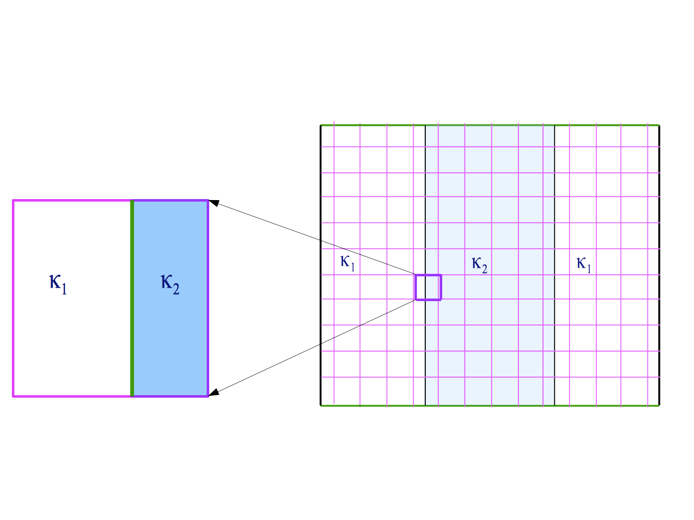
Figure 1: An example of a multimaterial grid. The rightmost figure shows a square numerical grid overlaid upon a rectangular physical geometry consisting of three parallel material regions with differing diffusion coefficients. The numerical grid partitions the physical geometry into a number of corresponding numerical cells, none of which need align with the material regions. The outer two regions are composed of the same material with diffusion coefficient $\kappa_{1}$, while the inner region has diffusion coefficient $\kappa_{2}$, forming a sandwich-like configuration. The planar sandwich test problem takes the outer two regions (the bread) to be nonconducting, with $\kappa_{1}=0$, while the inner region (the meat of the sandwich) conducts heat with $\kappa_{2}\equiv\kappa>0$. In the Figure, the numerical grid is misaligned relative to the material boundaries of the inner conducting region. This is illustrated in left panel figure.

Averaging techniques cannot always faithfully represent the physics of multimaterial cells. Consequently, FLAG employs more sophisticated multimaterial diffusion options, namely the thin mesh tm and static condensation sc algorithms. The thin mesh method starts with the volume fractions of each material region, and reconstructs the material interfaces using interface reconstruction methods. The mesh is then subdivided along the interfaces, making sure that the final polyhedral mesh conforms with the numerical mesh. This new unstructured mesh is constructed with full connectivity each cycle. The heat diffusion equation is solved on the subdivided mesh containing only single material cells.

The static condensation approach also makes use of the reconstructed material interfaces, but does not require all the details regarding connectivity across material interfaces within a cell. Instead, the global system for the diffusion equation is rewritten in terms of unknown face-centered temperature values. Total flux continuity is enforced at each cell face by ensuring that the sum of the fluxes from all materials on either side of the face are the same. There is an approximation here in that each cell face is assigned a single temperature associated with it; however, the fluxes contain the material-based diffusion coefficient $\kappa_{m}$, which are allowed to vary. The material-centered temperatures are eliminated from the system (via the Schur Complement), thus condensing the number of degrees of freedom. The global system is then solved for the unknown face temperatures using standard mimetic techniques. The result is that each cell now has a known solution on its boundary (faces), which becomes a local Dirichlet problem that can be solved independently to recover updated material-centered temperatures. For more details on the algorithm, see Ref. asc ; this method is reported to be second order accurate in Ref. sc .

II The Planar Sandwich Test Problem

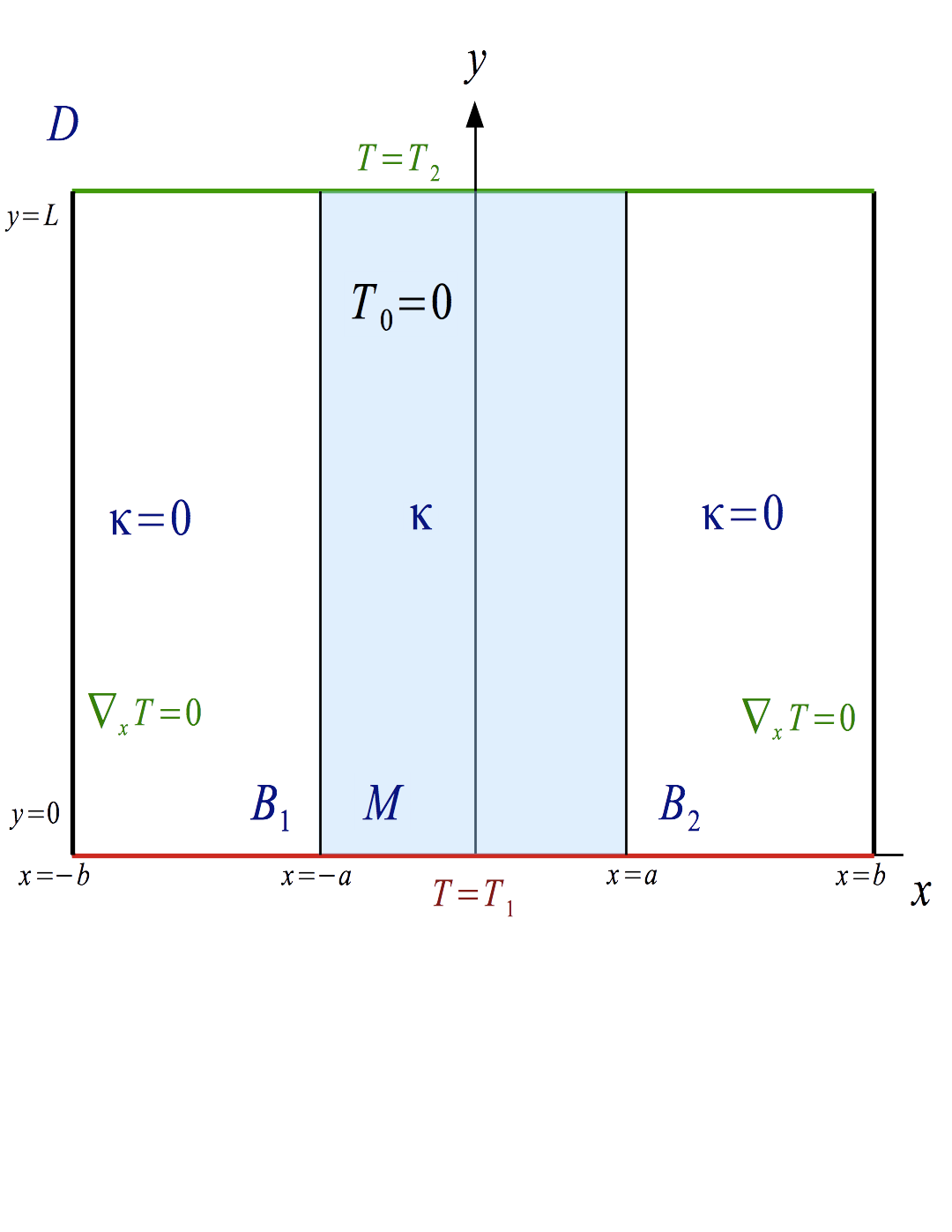
Figure 2: The Planar Sandwich is a 2D-Cartesian heat flow problem defined on the square domain $D=[0,L]\times[0,L]$. The temperature at location $(x,y)\in D$ at time $t$ is denoted by $T(x,y,t)$. The inner heat-conducing region $M=\{(x,y)\in D\,|\,a_{1}\leq x\leq a_{2}\}$, for which $\kappa>0$, is called the meat of the sandwich. The outer non-conducting materials, the bread of the sandwich, are located within $B_{1}=\{0\leq x<a_{1}\}$ or $B_{2}=\{a_{2}<x\leq L\}$, and are insulating, with $\kappa=0$. In numerical work, we take $\kappa=10^{-12}$ rather than zero. In setting the boundary conditions, we take the upper and lower boundary temperatures to be constant and uniform along $y=0$ and $y=L$ with values $T_{1}$ and $T_{2}$, respectively, i.e. we impose the Dirichlet boundary conditions $T(x,y=0,t)=T_{1}$ and $T(x,y=L,t)=T_{2}$. On the left and right boundaries, we take the temperature flux in the $x$-direction to vanish, i.e. we use the Neumann boundary conditions $\partial_{x}T(x=0,y,t)=0$ and $\partial_{x}T(x=L,y,t)=0$. We must also impose an initial condition: we set the temperature in the interior of the sandwich to zero, i.e. $T(x,y,t=0)=0$ for $(x,y)\in(0,L)\times(0,L)$. When $T_{1}>T_{2}$, heat flows in the $y$-direction from the lower to the upper boundary. This allows us to describe the planar sandwich in terms of 1D profiles $T(y,t)$. For numerical work, we take $a_{1}=0.75$ and $a_{2}=1.25$, or a shifted variant with $a_{1}=0.77$ and $a_{2}=1.27$.

This section is devoted to the planar sandwich test problem of Ref. DMS , as illustrated in Fig. 2. It is a 2D-Cartesian heat flow problem on the square domain $D=[0,L]\times[0,L]$, where the $x$-axis runs horizontally and the $y$-axis is vertical. We take $L=2$ (in arbitrary units) in all figures and examples that follow. The domain $D$ is partitioned into three vertical sandwich-like regions delimited by $x=a_{1}$ and $x=a_{2}$, with $0<a_{1}<a_{2}<L$. The inner region $a_{1}\leq x\leq a_{2}$ is composed of a heat-conduction material with heat diffusion coefficient $\kappa>0$, and is called the meat of the sandwich. The meat is surrounded by two non-heat conducting materials, called the bread of the sandwich, for which $\kappa=0$ in $0\leq x<a_{1}$ and $a_{2}<x\leq L$. Working in arbitrary temperature units, we wish to solve the 2D heat equation

$$\frac{\partial T}{\partial t} = {\bm{\nabla}}\cdot\Big{[}\kappa\,{\bm{\nabla}}T\,\Big{]}~{}~{}~{}{\rm for}~{}~{}(x,y)\in(0,L)\times(0,L)\ ,$$ (3)

where $T=T(x,y,t)$ is the temperature field at position $(x,y)$ and time $t$, with the diffusion coefficient taking the form

$$\kappa(x,y)=\left\{\begin{array}[]{ll}0&;~{}0\leq x<a_{1}\\[-5.0pt] \kappa&;~{}a_{1}\leq x\leq a_{2}\\[-5.0pt] 0&;~{}a_{2}<x\leq L\ .\end{array}\right.$$ (7)

The initial condition (IC) is chosen so that the temperature vanishes in the interior of the domain $D$ at time $t=0$,

$$T(x,y,0)=0~{}~{}~{}{\rm for}~{}~{}(x,y)\in(0,L)\times(0,L)\ ,$$ (8)

while the boundary conditions (BCs) are taken to be

$$T(x,0,t) = T_{1}\hskip 28.45274pt{\rm for}~{}~{}x\in[0,L]$$ (9)

$$T(x,L,t) = T_{2}$$ (10)

$$\partial_{x}T(0,y,t) = 0\hskip 34.14322pt{\rm for}~{}~{}y\in[0,L]$$ (11)

$$\partial_{x}T(L,y,t) = 0\ .$$ (12)

Note that the left- and right-hand sides of the rectangle are insulating, i.e. the temperature flux along the $x$-direction at the far left- and right-ends of $D$ vanishes, $\partial_{x}T(x=0,y,t)=0$ and $\partial_{x}T(x=L,y,t)=0$ for $0\leq y\leq L$. Along the lower and upper boundaries $y=0,L$, the temperature profiles are uniform in $x$ with $T(x,y=0,t)=T_{1}$ and $T(x,y=L,t)=T_{2}$, where $T_{1}$ and $T_{2}$ are constant temperature values over the length of the region $0\leq x\leq L$. When $T_{1}>T_{2}$, the Second Law of Thermodynamics ensures that heat flows upward from $y=0$ to $y=L$. We shall generalize the planar sandwich problem in Section V by considering nonhomogeneous boundary condition with nonzero heat flux and non-trivial initial conditions PlanarSandwichExactPackDoc .

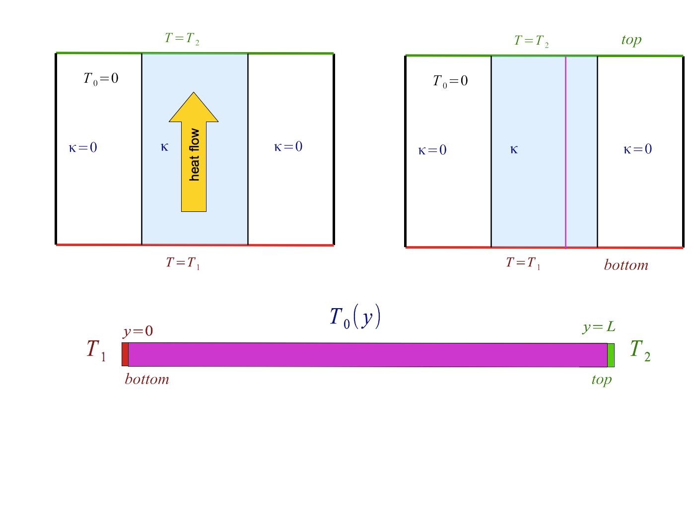
Figure 3: The 2D planar sandwich reduces to a 1D heat flow problem along a vertical rod of length $L$. In the top panels, the 2D temperature profile is a function of the $x$ and $y$ coordinates, $T=T(x,y,t)$. Since there is no $x$ dependence in the boundary conditions $T_{1}$ and $T_{2}$, the problem reduces to 1D temperature flow along the vertical direction, in which case $T=T(y,t)$ in the central heat-conducting region. To be consistent with the 2D geometrical setup, we will refer to the 1D boundary conditions $T(0,t)=T_{1}$ and $T(L,t)=T_{2}$ as the bottom and top boundary condition, respectively.

As illustrated in Fig. 3, the planar symmetry of the problem allows us to express the 2D solution in terms of a 1D profile along the $y$-direction, independent of the $x$-position within the central heat-conducting region $a_{1}\leq x\leq a_{2}$. This is because the upper and lower boundary conditions are uniform along the $x$-direction over the whole range $0\leq x\leq L$, and therefore heat flows only along the vertical direction. Thus, the corresponding 1D heat flow equation for $y$-the profile $T=T(y,t)$ is

$$\frac{\partial T}{\partial t} = \kappa\,\frac{\partial^{2}T}{\partial y^{2}}\ ,$$ (13)

where the 1D initial condition (IC) is

$$T(y,0)=T_{0}=0\ ,$$ (14)

and the corresponding 1D boundary conditions (BCs) are

$$T(0,t) = T_{1}\hskip 28.45274pt{\rm(bottom)}$$ (15)

$$T(L,t) = T_{2}\hskip 28.45274pt{\rm(top)}\ .$$ (16)

We refer to the BCs as the bottom and top boundary conditions, respectively, as suggested by the 1D rod in Fig. 3.

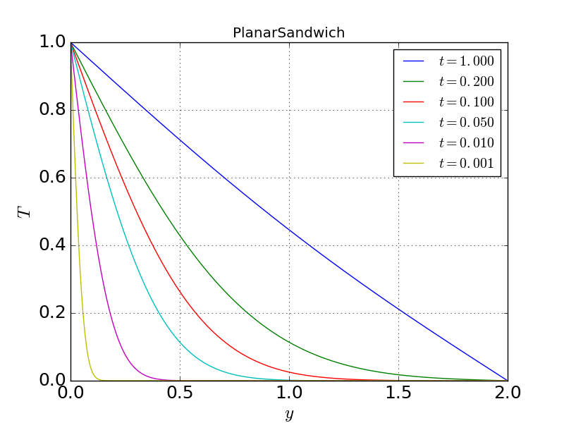
Figure 4: Temperature profiles $T(y,t)$ for the planar sandwich solution at six representative time slices, $t=0.001,0.01$, $0.05,0.1,0.2,1$, ranging from early to late times. The heat diffusion coefficient is taken to be $\kappa=1$, the length of the 1D heat-conducting rod is set to $L=2$ (the abscissa of the graph), and the the first 1000 terms of the series have been summed. We have employed the boundary conditions $T_{1}=1$, $T_{2}=0$ at $y=0$, $y=L$, with the initial condition $T_{0}=0$. Note that the solution at the earliest time $t=0.001$ has negligible temperature for all $y$ outside a small neighborhood about $y=0$, as required by the initial condition $T_{0}=0$. Also note that the late-time solution at $t=1$ is very close to the static equilibrium solution $\bar{T}(y)=T_{1}+(T_{2}-T_{1})\,y/L$. We shall perform all future verification analyses and convergence plots at time $t=0.1$. This time is early enough to capture the dynamics of the diffusive heat flow across a large range of $y$, and it is late enough to have a contribution from the static equilibrium solution.

The exact analytic solution for IC (14) and the BCs (15)–(16) was presented in Ref. DMS , and takes the form

$$T(y,t) = T_{1}+\frac{(T_{2}-T_{1})\,y}{L}+\sum_{n=1}^{\infty}B_{n}\,\sin(k_{n}\,y)\,e^{-\kappa\,k_{n}^{2}t}$$ (17)

$$k_{n} = \frac{n\pi}{L}\hskip 14.22636pt{\rm and}\hskip 14.22636ptB_{n}=\frac{2T_{2}\,(-1)^{n}-2T_{1}}{n\pi}\ .$$ (18)

The solution profiles $T(y,t)$ are plotted in Fig. 4 for six time slices $t=0.001,0.01,0.05$, $0.1,0.2,1$. The boundary conditions are $T_{1}=1$ and $T_{2}=0$, and the initial condition is $T_{0}=0$. We also take the diffusion constant to be $\kappa=1$, the length of the domain to be $L=2$, and we sum over the first 1000 terms of the series. As illustrated in Fig. 4, the solution at the earliest time $t=0.001$ has a negligible temperature for all values of $y$ outside a small neighborhood about $y=0$. Also note that the late-time solution at $t=1$ is very close to the static equilibrium solution

$$\bar{T}(y) = T_{1}+\frac{(T_{2}-T_{1})\,y}{L}\ .$$ (19)

We shall preform the verification analyses and convergence plots at time $t=0.1$. The choice $t=0.1$ is an intermediate time that is sensitive to both the dynamics of the heat flow and to the late-time equilibrium solution. This choice tests the static boundary conditions and the dynamics of the heat flow solver.

Even though we perform the FLAG simulations in a 2D cartesian geometry, we shall express the numerical solution in terms of its 1D profile. However, before proceeding, it is convenient to visualize the solutions in 2D. The $x$- and $y$-axes are divided into $N$ segments, with $N=5,10,20,40,80,160$. This gives the six grid spacings $h=0.5,0.2,0.1,0.05,0.025,0.0125$. Note that heat flows outside the boundary region, particularly at low resolutions. Figures 5 and 6 illustrate the arithmetic and harmonic average models for the 2D numerical FLAG solutions, for six levels of increasing resolution. To better understand these Figures, we examine the arithmetic technique in more detail. We shall see that the arithmetic average has the effect of extending the inner material beyond the boundary, while the harmonic average decreases the inner material within the boundary. For the planar sandwich geometry illustrated in Fig. 1, the material boundaries are static with $x=a_{1}$ and $x=a_{2}$. The arithmetic average of the diffusion coefficient on a boundary cell is

$$\bar{\kappa}_{a} = V_{1}\,\kappa_{1}+V_{2}\,\kappa_{2}=V_{1}\,\epsilon+V_{2}\,\kappa\to V_{2}\kappa>0\ ,$$ (20)

and we should expect the arithmetic average to overestimate the effects of multimaterial heat flow along the boundary cells.

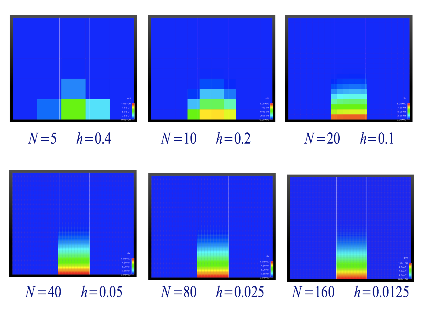
Figure 5: Illustration of the 2D planar sandwich solution employing the arithmetic average multimaterial algorithm for six resolutions. The $x$- and $y$-axes are divided into $N$ segments, with $N=5,10,20,40,80,160$. For $L=2$ this gives the six resolutions $h=0.5,0.2,0.1,0.05,0.025,0.0125$. Note that heat flows outside the central boundary region $a_{1}=0.77\leq x\leq 1.27=a_{2}$. This is particularly noticeable at low resolutions.

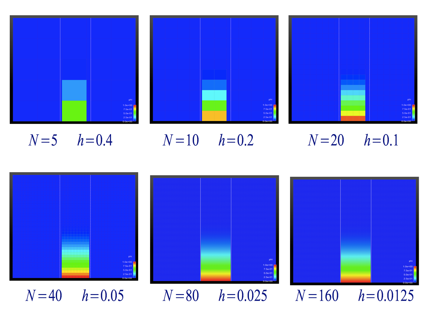
Figure 6: Illustration of the 2D planar sandwich solution employing the harmonic average multimaterial algorithm for six resolutions. The $x$- and $y$-axes are divided into $N$ segments, with $N=5,10,20,40,80,160$. For $L=2$ this gives the six resolutions $h=0.5,0.2,0.1,0.05,0.025,0.0125$. Note that the heat is underestimated in the multimaterial regions.

Conversely, the harmonic average gives

$$\bar{\kappa}_{h}^{-1} = V_{1}\,\kappa_{1}^{-1}+V_{2}\,\kappa_{2}^{-1}=V_{1}\,\epsilon^{-1}+V_{2}\,\kappa^{-1}\to V_{1}\epsilon^{-1}~{}~{}{\rm or}~{}~{}\bar{\kappa}_{h}\to 0\ ,$$ (21)

which underestimates the effects of multimaterial heat flow along the boundary cells. The numerical FLAG results of Ref. DMS indeed show that the arithmetic mean emphasizes larger values of the diffusion coefficient, while the harmonic mean emphasizes smaller values.

III Using ExactPack Heat Solvers

In this section we present an example of how to use ExactPack exactpack to perform code verification for the exact solution of the planar sandwich.  One starts by importing the planar sandwich solution module into Python,

from exactpack.solvers.heat import PlanarSandwich

As discussed in the last section, the exact solution for the 2D planar sandwich can be described in terms of a 1D rod of length $L$ with a uniform heat diffusion coefficient $\kappa$. The 1D solution is implemented in ExactPack by the solver PlanarSandwich. The planar sandwich class comes with a number of default settings for the input parameters, such as the length of the rod, the value of the heat diffusion coefficient, settings for the boundary and initial conditions, and the number of terms to be summed in the series. To instantiate and use the PlanarSandwich class with default values, one invokes

solver = PlanarSandwich()

The parameter values can be explicitly set by

solver = PlanarSandwich(T1=1, T2=0, L=2, kappa=1, Nsum=1000)

This creates an ExactPack object called solver with boundary conditions $T_{1}=1$ and $T_{2}=0$, the length of the 1D rod set to $L=2$, the diffusion coefficient set to $\kappa=1$, and we have specified that we want to retain the first 1000 terms in the summation. The default initial condition is $T_{0}=0$; this can be changed by setting the variables TA and TB. Access to all the properties of the planar sandwich definition can be controlled through the class PlanarSandwich.

The planar sandwich object encapsulates the definition of the problem, but it is unaware of the spatial grid necessary for a specific realization of the problem. Therefore, a solver object must be used to produce a solution object on a spatial array at a given time t=0.1. The corresponding Python code is

solver = PlanarSandwich()

L = 2
y = numpy.linspace(0, L, 1000)
t = 0.1

soln = solver(y, t)
soln.plot(’temperature’)

The solver object solver takes a spatial array y and a time variable t, and produces a solution object called soln with the exact solution evaluated on the spatial array at the given time. As illustrated by the last line above, a solution object is equipped with a plotting method, in addition to various analysis methods not shown here. The Python script that produces Fig. 4 is given in Appendix A, and is summarized in Fig. 7.

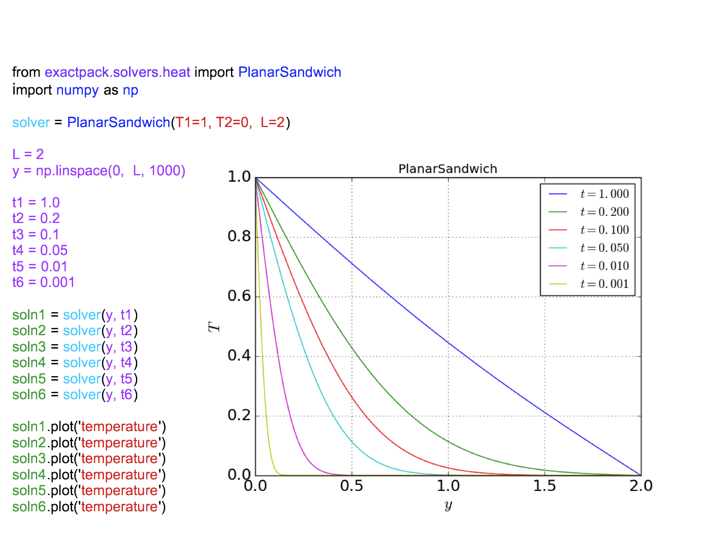
Figure 7: An illustration of the Python source code used to plot the planar sandwich contour solutions of Fig. 4. The Python script to produce this figure is provided in Appendix A. The planar sandwich solver has been instantiated by solver = PlanarSandwich(T1=1, T2=0, L=2), which sets the boundary conditions to $T(0,t)=1$, $T(L,t)=0$, the initial condition to $T(y,0)=0$, and the length of the rod (along the $y$-direction) to $L=2$. The values $\kappa=1$ and $N_{\rm sum}=1000$ are the default settings, and are not specified in the above code segment. The solver is used to form a solution object from a spatial array y and a time t by soln = solver(y, t).

IV Grid Resolution Studies of the Planar Sandwich

In the previous sections, we examined the planar sandwich test problem in some detail, in particular, we provided the exact solution in a semi-analytic form in Eq. (17). The geometry of the planar sandwich is illustrated in Fig. 1, and the material interfaces and their heat conduction properties are defined in Fig. 2. In this section, we build on these results by performing rigorous convergence analyses for the four primary multimaterial heat flow algorithms in FLAG, namely, (i) the arithmetic average, (ii) the harmonic average, (iii) thin mesh, and (iv) static condensation. As we have already emphasized, the analyses are performed at time $t=0.1$, and the domain of the planar sandwich is the two dimensional region $D=[0,L]\times[0,L]$. In numerical simulations we take $L=2$, partitioning the domain $D$ into $N\times N$ square cells with sides of length $h=L/N$. In other words, the 2D computational grid is formed by dividing the $x$- and $y$-grids into $N$ equal segments of length $h$, thereby creating $N^{2}$ square cells with sides of length $\Delta x=\Delta y=h$. It should be noted that the algorithms in FLAG do not require the cells to be square, and all multimaterial methods work on general polytopal meshes. We only use square cells to provide a unique length scale $h$ with which to plot the norms. In all numerical simulations, we take the number of segments to increase by a factor of two, starting with five segments for the lowest resolution and ending with 640 for the highest resolution,

$$N=5,10,20,40,80,160,320,640\ .$$ (22)

For $L=2$, the square cells have sides of length

$$h\equiv L/N=0.4,0.2,0.1,0.05,0025,0.0125,0.00625,0.003125.$$ (23)

It is important to note that in all numerical simulations, we halve the maximum time step for every doubling in $N$. The central heat-conducting material, the meat of the sandwich, is the 2D region $M=\big{\{}(x,y)\in D\,|\,a_{1}\leq x\leq a_{2}~{}{\rm and}~{}0\leq y\leq L\big{\}}$, within which the heat diffusion coefficient takes the value $\kappa=1$. The outer two materials $B=\big{\{}(x,y)\in D\,|\,0\leq x<a_{1}~{}{\rm or}~{}a_{2}<x\leq L~{}{\rm with}~{}0\leq y\leq L\big{\}}$ are called the bread of the sandwich, and are composed of an insulated material for which $\kappa=0$. In our numerical simulations, we do not actually take the heat diffusion coefficient to vanish inside $B$, but rather, we set $\kappa=\epsilon\equiv 10^{-12}$. We should therefore think of the condition $\kappa=10^{-12}$ as a limiting procedure in which $\kappa=\epsilon$ with $\epsilon\to 0^{+}$.

IV.1 The Arithmetic Average

In this section we perform the convergence analysis for the arithmetic average multimaterial algorithm in FLAG. We first consider the case in which $a_{1}=0.75$ and $a_{2}=1.25$ (with $L=2$). At grid point $(x_{i},y_{j})\in D$ and time $t=0.1$, the numerical algorithm returns a temperature $T_{ij}$, and therefore, the numerical results can be expressed by the $N^{2}$ triplets $(x_{i},y_{j},T_{ij})$ for $i,j=1,2\cdots N$. In Fig. 8, we have projected out the $x$-coordinate and plotted the points $(y_{j},T_{ij})$ at time $t$. Note that the numerical solutions becomes more finely spaced in $y$ with increasing $x$-resolution, until the points $(y_{j},T_{ij})$ lie on top of the exact 1D profile $T(y,t)$. In the Fig. 8, the exact solution is the solid black line, although it is difficult to resolve against the dense numerical background.

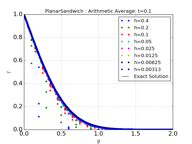
Figure 8: The numerical FLAG runs for the planar sandwich at time $t=0.1$ for the arithmetic average technique. The exact solution is plotted in black, although it is difficult to resolve against the dense numerical background. We have performed numerical runs for $N=5,10$, $20,40,80,160,320,640$. Choosing length $L=2$, the corresponding resolutions are $h\equiv N/L=0.4$, $0.2,0.1,0.05,0025,0.0125,0.00625,0.003125$. For every resolution $h$, the numerical solution can be expressed by the triplets $(x_{i},y_{j},T_{ij})$ for $i,j=1,2\cdots N$. We have projected out the $x$-coordinates, plotting $(y_{j},T_{ij})$ in the Figure. At high resolutions, the solution becomes independent of $x_{i}$, and indeed, as the grid resolution increases, the points become more closely spaced, and lie closer to the exact solution. For these numerical runs, we have taken the conducting region (the meat of the sandwich) to be $a_{1}=0.75\leq x\leq 1.25=a_{2}$. The numerical results for the shifted region $a_{1}=0.77\leq x\leq 1.27=a_{2}$ are qualitatively similar in appearance.

Let us examine the ExactPack script used to produce Fig. 8. ExactPack contains an object called Study that, among other things, can be used to plot the numerical data alongside the exact solution:

study = Study(datasets=dumpfiles,
    reference=PlanarSandwich(),
    study_parameters=[0.4, 0.2, 0.1, 0.05, 0025, 0.0125, 0.00625, 0.003125],
    time=0.1,
    reader=FlagVarDump(),
    abscissa=’y_position’
    )

study.plot(’temperature’)

The statement study=Study($\cdots$) instantiates the object Study by the instance study, where the latter inherits it properties and methods from the former. The study object contains a plot method, study.plot(’temperature’), which instructs the object to plot itself, thereby producing Fig. 8. The object Study() takes a number of arguments. The first argument datasets has been assigned the value dumpfiles, which is a regular expression for the path of the code output. The output consists of separate code runs at the resolutions specified by study_parameters and at the time specified by time. The argument reference is used to select the reference solver in ExactPack, which in this case is PlanarSandwich. The argument reader provides the interface between the code output and ExactPack. In this case, the code reader is specific to FLAG; however, ExactPack will soon use the VTK format by default. In general, the numerical output can always be expressed in the form $(x_{i},y_{j},T_{ij})$ with $i,j,=1,\cdots,N$, for every resolution $N$, and the final argument abscissa=‘y_position‘ specifies that only data only along the $y$-direction be used in the analyses. With this setting, the analyses and figures are performed using the 1D profile representation. The ExactPack script and corresponding Figure are summarized in Fig. 9, with the upper left margin specifying the ExactPack script.

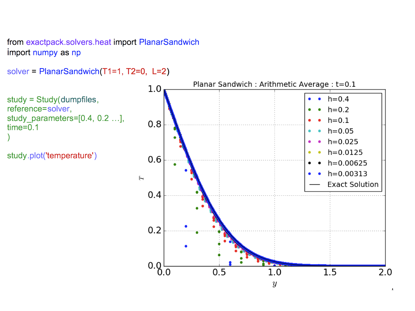
Figure 9: A summary of the Python source code used to produce Fig. 8. The exact solution is plotted in black, although it is hard to resolve against the dense numerical background. The study object contains a plotting method that plots the exact solution alongside the numerical results.

The $L_{1}$ error norm is defined by

$$L_{1}=\sum_{i,j=1}^{N}\,\bigg{|}T_{ij}^{\,\rm num}-T_{ij}^{\,\rm ex}\bigg{|}\ ,$$ (24)

where $T_{ij}^{\rm num}=T_{ij}$ is the numerical solution at position $(x_{i},y_{j})$ and time $t$, and $T_{ij}^{\rm ex}=T(x_{i},y_{j},t)$ is the corresponding exact solution. We remind the reader that we take $t=0.1$ in all numerical analyses, simulations, and figures. We can define a restricted metric $L_{1}(R)$ over a subset $R\subset D$, such that

$$L_{1}(R)=\!\sum_{ij,\,(x_{i},y_{j})\in R}\,\bigg{|}T_{ij}^{\,\rm num}-T_{ij}^{\,\rm ex}\bigg{|}\ .$$ (25)

ExactPack currently only supports the data format of the 1D profile along $y$; therefore, the norms are only calculated over 1D regions $R\subset(0,L)$ along the $y$-axis,

$$L_{1}(R)=\sum_{ij,\,y_{j}\in R}\bigg{|}T_{ij}^{\,\rm num}-T_{ij}^{\,\rm ex}\bigg{|}\ .$$ (26)

Since the temperature vanishes inside region $B$, the only sizable contributions to $L_{1}$ occur for $(x_{i},y_{j})\in M$.

Figure 10 illustrates the convergence analysis for the planar sandwich test problem in FLAG, where we have plotted the $L_{1}$ norm against the resolution $h$ on a log-log scale. For the heat-conducting region delimited by $a_{1}=0.75\leq x\leq 1.25=a_{2}$ with $L=2$ and $N=5$, the $4^{\rm th}$ mesh refinement has resolution $h=0.05$, at which point the numerical grid aligns with the material boundaries at $x=a_{1}$ and $x=a_{2}$. At the alignment, the accuracy of the code increases by over an order of magnitude, thereby giving rise to a discontinuity in the convergence plot. Note, however, that the upper and lower branches converge at approximately the same rate $p=1.2$. As shown in Fig. 11, we can eliminate the discontinuity by slightly shifting the conduction region to $a_{1}=0.77\leq x\leq 1.27=a_{2}$, in which case the grid points of the shifted region never align with a material interfaces. As we see in the lower panel of the Figure, the convergence rate is $p=1.0$. In everything that follows, we use the shifted region by default. Before continuing, we provide a brief summary of the ExactPack code used to create the convergence study of Fig. 10:

domain = (0, L)
fiducials = {’temperature’: 1}
fit = RegressionConvergenceRate(study, domain=domain fiducials=fiducials)
fit[0:3].plot_fit(’temperature’, "-", c=’b’)
fit[3:8].plot_fit(’temperature’, "-", c=’r’)
fit.norms.plot(’temperature’)
fit.plot_fiducial(’temperature’)
fit.plot(’temperature’)

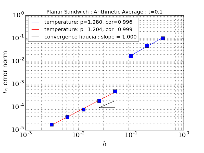
Figure 10: Convergence analysis at time $t=0.1$ for the planar sandwich using the arithmetic average treatment of multimaterial cells. The length of the domain is $L=2$ with eight uniform regions $N=5,10,20,40,80,160,320,640$, corresponding to resolutions $h=0.4,0.2,0.1,0.05,0025$, $0.0125,0.00625,0.003125$. Since $a_{1}=0.75\leq x\leq 1.25=a_{2}$ with $L=2$, the numerical grid and the material interface align on the the $4^{\rm th}$ iteration at $h=0.05$. When the mesh aligns with the material boundary, the accuracy increases by an order of magnitude, producing a discontinuity in the convergence graph. However, both the upper and lower branches converge at approximately the same rate.

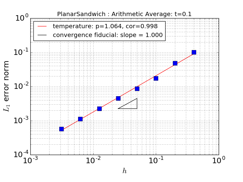
Figure 11: The convergence analysis in FLAG at time $t=0.1$ for the planar sandwich using the arithmetic average treatment of multimaterial cells gives $p=1.0$. The length of the domain is $L=2$ with eight uniform regions $N=5,10,20,40,80,160,320,640$, corresponding to resolutions $h=0.4,0.2,0.1,0.05,0025$, $0.0125,0.00625,0.003125$. The central region has been shifted to $a_{1}=0.77\leq x\leq 1.27=a_{2}$, so that the mesh refinements are never commensurate with this region. The convergence plot is then rendered continuous.

The above script starts with the assignment statement domain = (0,L), which specifies the region along $y$ over which to calculate the norm, where, as usual, we take $L=2$. The command fiducials = {’temperature’: 1} defines a Python dictionary that sets the slope of the fiducial triangle to unity. The next line, fit = RegressionConvergenceRate($\cdots$), instantiates the convergence rate object RegressionConvergenceRate by the instance fit. The object RegressionConvergenceRate performs a convergence analysis based on an error Ansatz $L_{1}(h)=A\,h^{p}$, and it takes the following arguments: the object study discussed above, the domain over which the norm is calculated, and the fiducial dictionary. The command fit.plot_fit exercises the method plot_fit, which uses the matplotlib.pyplot.plot routine to plot the error norms and the best fit convergence rate for the error Ansatz. Other error Ansatze can be used if desired. Since the convergence rate is discontinuous at the $4^{\rm th}$ iteration in resolution, we use the nomenclature fit[0,3] and fit[3,8] to perform the fits on the first three and last five data sets independently, thereby giving convergence rates for the upper and lower branches. It is necessary to do an explicit matplotlib.pyplot.show to display the plot, fit.plot(‘temperature‘). Figure 12 summarizes the results of this section.

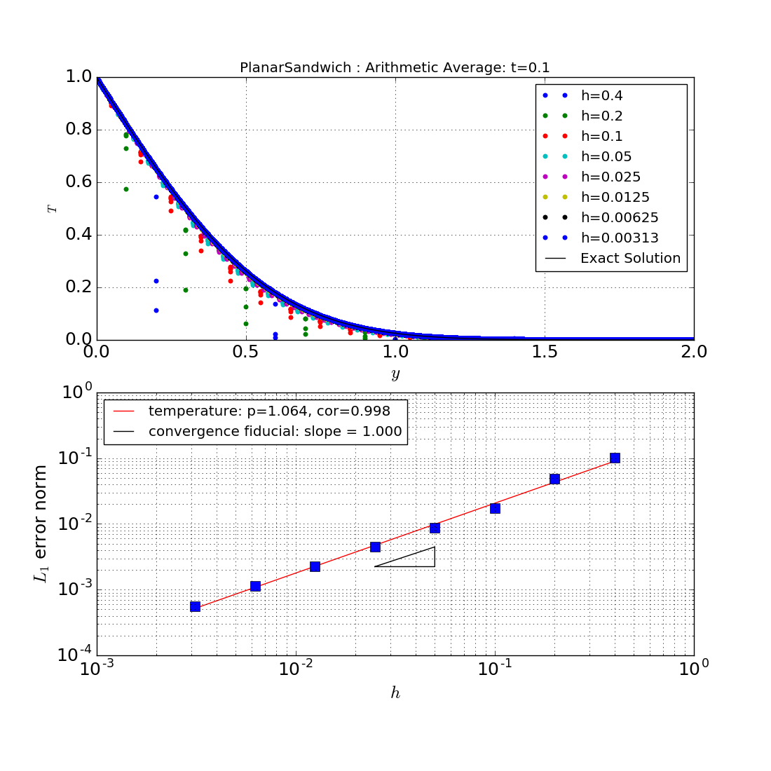
Figure 12: The arithmetic average for multimaterial cells. Numerical profiles at time $t=0.1$ are show in the top panel, and the convergence analysis in the bottom panel, corresponding to Figs. 10 and 11. The length of the domain is $L=2$ for eight uniform segments with $N=5,10,20,40,80,160,320,640$, corresponding to resolutions $h=0.4,0.2,0.1,0.05,0025,0.0125$, $0.00625,0.003125$. The central heat-conducting region has been shifted to $a_{1}=0.77\leq x\leq 1.27=a_{2}$, so that the mesh refinements never align with a material boundary. The convergence rate for the arithmetic average is approximately $p=1$.

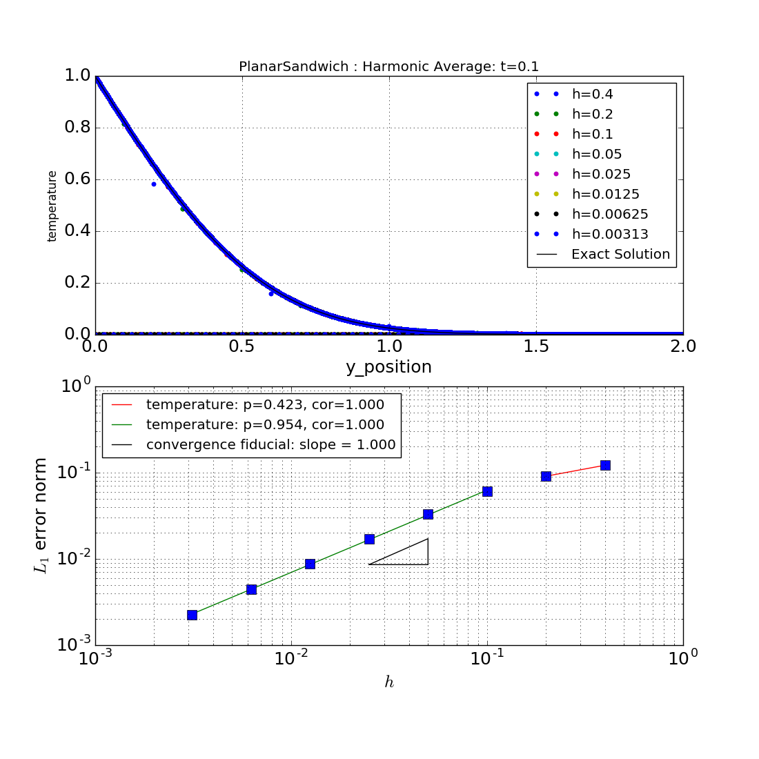
Figure 13: The harmonic average for multimaterial cells. The parameter setting are the same as in Fig. 12.

IV.2 The Harmonic Average

We now perform a convergence analysis for the harmonic average multimaterial model in FLAG. As discussed in the previous section, it is convenient to use the shifted heat-conducting region delimited by $a_{1}=0.77\leq x\leq 1.27=a_{2}$, where the length of the domain is take to be $L=2$. In this way, the numerical grid never aligns with the material interfaces at $x=a_{1}$ and $x=a_{2}$, thereby rendering the convergence plot continuous. Figure 13 illustrates the convergence analysis for the harmonic average. The upper panel of the Figure plots the numerical solutions $(y_{j},T_{ij})$ alongside the exact 1D profile, and the lower panel gives the corresponding convergence analysis. Note that the first two points, $N=5,10$, converges at a rate $p=0.4$, while $N=20,40,\cdots,640$ converges approximately linearly with $p=0.95$, indicating that the first two points lie outside the asymptotic range of convergence. Comparing the upper panels of Figs. 12 and 13, we see that the harmonic average solutions do not have the same degree of scattering as the arithmetic average, and they lie much closer to the exact analytic profile. Note, however, that the harmonic average solutions contain a spurious branch along the horizontal axis. This arises because of a bug in FLAG, which fails to propagate the heat flow on a small number of discrete grid points.

IV.3 Thin Mesh and Static Condensation

Figure 14: The thin mesh option for multimaterial cells. The parameter setting are the same as in Fig. 12.

We now turn to the more advanced multimaterial algorithms of FLAG, namely, thin mesh tm and static condensation sc . As discussed in the Introduction, the thin mesh algorithm uses the volume fractions of each material to reconstruct the material interfaces by employing interface reconstruction methods. The mesh is then subdivided along the interfaces, making sure that the final polyhedral mesh conforms with the numerical mesh. This method is quite accurate but very time consuming. Figure 14 illustrates the analysis, with the upper panel showing the numerical solutions plotted alongside the exact solution, and the lower panel giving the convergence plot. Note that thin mesh starts out with $2^{\rm nd}$ order convergence, $p=2$, and becomes lower order order as the mesh resolution is refined, eventually giving $p=1$ at the smallest resolutions. There are a number of possible reasons why the convergence rate levels off as the grid is refined, and we are currently investigating this. One possibility is that the order of accuracy is limited by the interface reconstruction algorithm critical to both of these methods.

The static condensation approach also makes use of the reconstructed material interfaces, but does not require the connectivity information across material interfaces within a cell. The global system for the diffusion equation is rewritten in terms of unknown face-centered temperature values, and flux continuity is enforced at each cell face by ensuring that the sum of the fluxes from all materials on either side of the face are the same. The global system is then solved for the unknown face temperatures. The result is that each cell now has a known solution on its boundary (faces), which becomes a local Dirichlet problem that can be solved independently to recover updated material-centered temperatures. For more details on the algorithm, see Ref. asc ; this method is reported to be second order accurate in Ref. sc . Figure 15 illustrates the analysis for static condensation, which exhibits quantitatively similar scaling to thin mesh. In fact, for the planar sandwich test problem, static condensation agrees with thin mesh almost exactly.

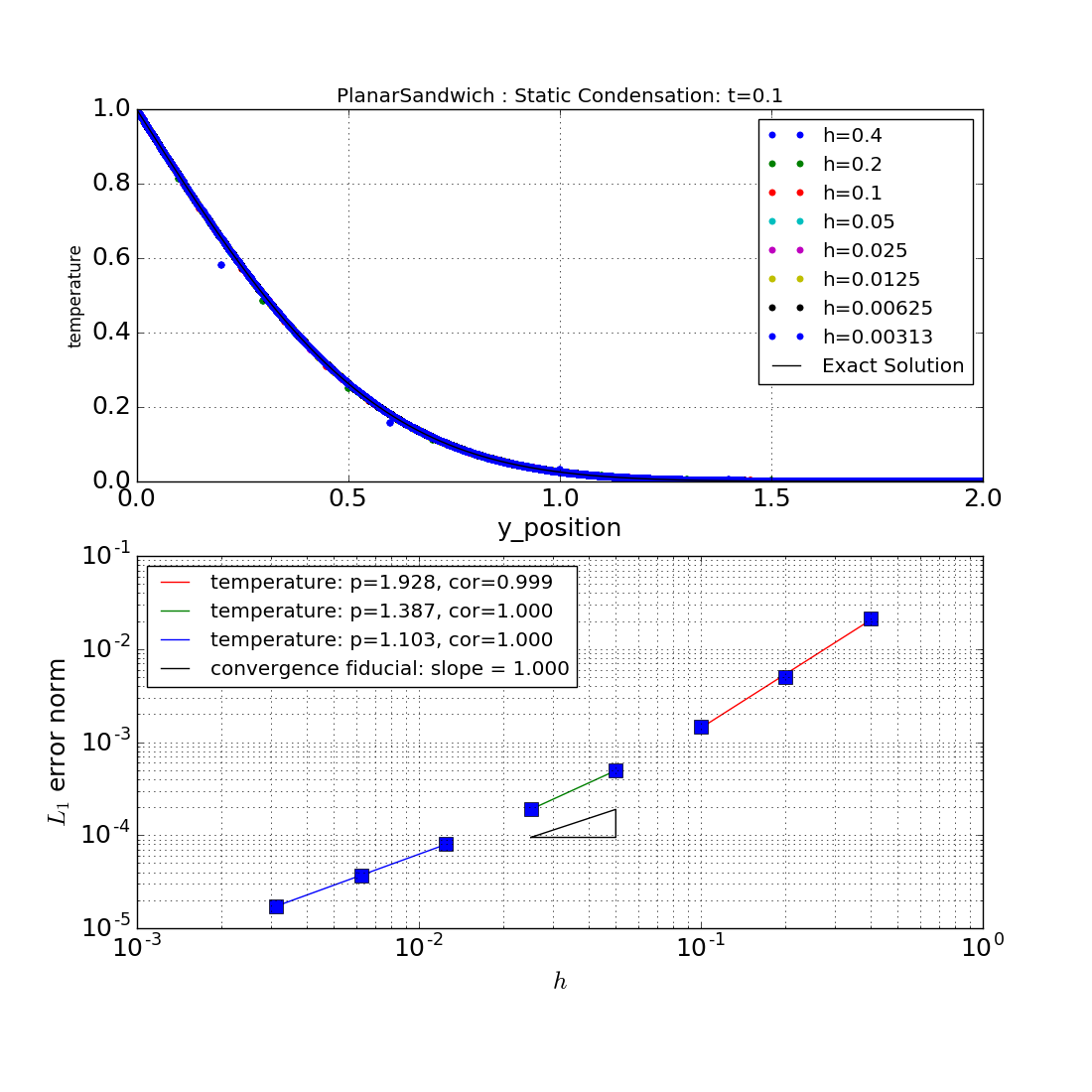
Figure 15: The static condensation option for multimaterial cells. The parameter setting are the same as in Fig. 12.

V Generalizations of the Planar Sandwich

As we have seen, the 2D planar sandwich test problem can be expressed in terms of heat flow along a 1D rod oriented in the horizontal direction, as illustrated in Fig. 3. The planar sandwich is a special case of the more general heat flow problem Berg ,

$$\frac{\partial T(y,t)}{\partial t} = \kappa\,\frac{\partial^{2}T(y,t)}{\partial y^{2}}$$ (27)

$$\alpha_{1}T(0,t)+\beta_{1}\partial_{y}T(0,t) = \gamma_{1}$$ (28)

$$\alpha_{2}T(L,t)+\beta_{2}\partial_{y}T(L,t) = \gamma_{2}$$ (29)

$$T(y,0) = T_{0}(y)\ .$$ (30)

This problem is implemented by the ExactPack class Rod1D. We use an arbitrary but consistent set of temperature units. Equation (27) is a diffusion equation describing the temperature response to heat flow in a material with constant diffusivity. The next two equations, Eqs. (28) and (29) are the boundary conditions (BCs), which we take to be nonhomogeneous linear combinations of Dirichlet and Neumann conditions. The initial condition (IC) is given by Eq. (30), and specifies the $t=0$ temperature profile along the rod. When the right-hand sides of the BCs vanish, $\gamma_{1}=\gamma_{2}=0$, the problem is called homogeneous, otherwise the problem is called nonhomogeneous. The distinction between homogenous and nonhomogeneous solutions has far-reaching implications for how one goes about solving the heat problem. The special property of homogeneous solutions is that the sum of any two homogeneous solutions is another homogeneous solution. However, such linearity is not true for nonhomogeneous solutions, as adding two nonzero values of $\gamma_{i}$ violates the BCs.

Finding a solution to the general problem (27)–(30) involves solving both the homogeneous and nonhomogeneous problems. The general homogenous solution, for which $\gamma_{1}=\gamma_{2}=0$, will be denoted by $\tilde{T}(y,t)$. To construct the exact solution, we must also find a specific static solution to the nonhomogeneous problem, which we denote by $\bar{T}(y)$. The general solution therefore takes the form

$$T(y,t)=\tilde{T}(y,t)+\bar{T}(y)\ .$$ (31)

The homogeneous solution $\tilde{T}(y,t)$ will be expressed as a Fourier series, and its coefficients will be chosen so that the initial condition (30) is satisfied by $T(y,t)$. This means that we choose the Fourier coefficients of $\tilde{T}$ such that

$$\tilde{T}(y,0)=T_{0}(y)-\bar{T}(y)\ .$$ (32)

The static nonhomogeneous solution $\bar{T}(y)$ is itself linear in $y$, and takes the form

$$\bar{T}(y;T_{1},T_{2}) = T_{1}+\frac{T_{2}-T_{1}}{L}\,y\ ,$$ (33)

where the temperatures $T_{1}$ and $T_{2}$ are defined in terms of the parameters $\alpha_{i}$, $\beta_{i}$, and $\gamma_{i}$ for $i=1,2$. Although there exists a solution to the heat flow equations for any continuous initial condition $T_{0}(y)$, it is convenient for our purposes to consider only the linear initial condition

$$T_{0}(y;T_{\scriptscriptstyle\rm A},T_{\rm\scriptscriptstyle B})=T_{\scriptscriptstyle\rm A}+\frac{T_{\rm\scriptscriptstyle B}-T_{\scriptscriptstyle\rm A}}{L}\,y\ ,$$ (34)

for independent temperature parameters $T_{\scriptscriptstyle\rm A}$ and $T_{\rm\scriptscriptstyle B}$. This form can also be used for the flux boundary condition $\partial_{y}T(L)=F_{\rm\scriptscriptstyle B}$ by setting $T_{\rm\scriptscriptstyle B}=F_{\rm\scriptscriptstyle B}L$. Therefore, (32) can be written as

$$\tilde{T}(y,0) = T_{0}(y)-\bar{T}(y)$$ (35)

$$= T_{a}+\frac{T_{b}-T_{a}}{L}\,y\ ,$$ (36)

where

$$T_{a} = T_{\scriptscriptstyle\rm A}-T_{1}$$ (37)

$$T_{b} = T_{\rm\scriptscriptstyle B}-T_{2}\ .$$ (38)

By assuming a linear IC, we find that the boundary conditions and initial conditions can be interchanged according to (37) and (38). It would be an interesting verification exercise to observe the extent to which this holds true in a code, since code algorithms handle boundary and initial conditions quite differently.

Let us briefly discuss some basic issues involving uniform convergence Rubin . This is related to order-of-limits questions in classical mathematics, which have direct practical implications for many mathematical systems of interest. The parameters $T_{\scriptscriptstyle\rm A}$ and $T_{\rm\scriptscriptstyle B}$ specify the initial temperatures at the bottom and top of the rod, or the bottom and top of the 1D slice in Fig. 3. By bottom and top, we really mean the limits $y=0^{+}$ and $y=L^{-}$, respectively. In other words, the linear initial condition $T_{0}(y)$ is defined only on the open interval $(0,L)$, with $T_{\scriptscriptstyle\rm A}$ being the value of $T_{0}(y)$ as $y\to 0^{+}$ and $T_{\rm\scriptscriptstyle B}$ being the value of $T_{0}(y)$ as $y\to L^{-}$. The temperatures $T_{\scriptscriptstyle\rm A}$ and $T_{\rm\scriptscriptstyle B}$ need not be equal to the boundary conditions $T_{1}$ and $T_{2}$. If the BCs and the IC do not agree, then the solution is nonuniformly convergent for $t\to 0$. As an example, consider BC1 with $T_{1}\neq T_{\scriptscriptstyle\rm A}$ and $T_{2}\neq T_{\rm\scriptscriptstyle B}$. The profile $T(y,t)$ converges point-wise to the initial profile $T_{0}(y)$ as $t$ goes to zero over the domain $(0,L)$, that is to say, the temperature $T(y,t)\to T_{0}(y)$ as $t\to 0$ for all $y\in(0,L)$. However, this point-wise convergence in $y$ is nonuniform on the closed interval $[0,L]$, in that $T(0,t)=T_{1}\neq T_{\scriptscriptstyle\rm A}$, although $\lim_{y\to 0^{+}}T(y,t)=T_{\scriptscriptstyle\rm A}\neq T_{\scriptstyle 1}=T(0,t)$. Similarly, $\lim_{y\to L^{-}}T(y,t)\neq T(L,t)$. These conditions place a limit on how close to $t=0$ one can set the time $t$ in convergence plots. See Ref. Rubin for an introductory but solid treatment of real analysis and nonuniform convergence.

The boundary conditions (28) and (29) are specified by the coefficients $\alpha_{i}$, $\beta_{i}$, and $\gamma_{i}$ for $i=1,2$. These parameters are not all independent, and various combinations will produce the same temperatures $T_{i}$ and fluxes $F_{i}=\partial_{y}T_{i}$; therefore, it is often more convenient to specify the boundary conditions directly in terms of $T_{i}$ and $F_{i}$. For example, if $\beta_{1}=0$ in (28), then the boundary condition becomes $\alpha_{1}T(0,t)=\gamma_{1}$, which we can rewrite in the form $T(0,t)=T_{1}$ with $T_{1}=\gamma_{1}/\alpha_{1}$. There are four special boundary conditions that provide particularly simple solutions. The first class is specified by $\beta_{1}=\beta_{2}=0$ with $\alpha_{i}\neq 0$, and gives the Dirichlet boundary conditions

$${\rm BC1}$$

$$T(0,t)=T_{1}\hskip 5.69046pt:~{}\hskip 4.26773pt\alpha_{1}\neq 0\hskip 14.22636pt\beta_{1}=0\hskip 28.45274ptT_{1}=\frac{\gamma_{1}}{\alpha_{1}}$$ (39)

$$T(L,t)=T_{2}~{}:~{}\hskip 4.26773pt\alpha_{2}\neq 0\hskip 14.22636pt\beta_{2}=0\hskip 28.45274ptT_{2}=\frac{\gamma_{2}}{\alpha_{2}}\ .$$ (40)

The planar sandwich of the previous sections is a subclass of BC1. The next class of boundary conditions is obtained by by setting $\alpha_{1}=\alpha_{2}=0$ with $\beta_{i}\neq 0$, and this gives the Neumann boundary conditions

$${\rm BC2}$$

$$\partial_{y}T(0,t)=F_{1}\hskip 5.69046pt:~{}\hskip 4.26773pt\alpha_{1}=0\hskip 14.22636pt\beta_{1}\neq 0\hskip 28.45274ptF_{1}=\frac{\gamma_{1}}{\beta_{1}}$$ (41)

$$\partial_{y}T(L,t)=F_{2}~{}:~{}\hskip 4.26773pt\alpha_{2}=0\hskip 14.22636pt\beta_{2}\neq 0\hskip 28.45274ptF_{2}=\frac{\gamma_{2}}{\beta_{2}}\ .$$ (42)

Since the differential equation does not contain sources or sinks of heat, energy conservation requires that we must further constrain the heat fluxes to be equal, $F_{1}=F_{2}\equiv F$. In other words, the heat flowing into the system must equal the heat flowing out of the system. We will refer to such solutions as the hot and warm planar sandwiches, depending on whether $F=0$ or $F\neq 0$. The final two classes of BCs are mixed Dirichlet and Neumann conditions,

$${\rm BC3}$$

$$T(0,t)=T_{1}\hskip 18.49411pt:\hskip 7.11317pt\alpha_{1}\neq 0\hskip 14.22636pt\beta_{1}=0\hskip 28.45274ptT_{1}=\frac{\gamma_{1}}{\alpha_{1}}$$ (43)

$$\partial_{y}T(L,t)=F_{2}~{}:~{}\hskip 4.26773pt\alpha_{2}=0\hskip 14.22636pt\beta_{2}\neq 0\hskip 28.45274ptF_{2}=\frac{\gamma_{2}}{\alpha_{2}}\ ,$$ (44)

and

$${\rm BC4}$$

$$\partial_{y}T(0,t)=F_{1}~{}:~{}\alpha_{1}=0\hskip 15.6491pt\beta_{1}\neq 0\hskip 28.45274ptF_{1}=\frac{\gamma_{1}}{\beta_{1}}$$ (45)

$$T(L,t)=T_{2}\hskip 12.80365pt:~{}\hskip 2.27626pt\alpha_{2}\neq 0\hskip 14.22636pt\beta_{2}=0\hskip 28.45274ptT_{2}=\frac{\gamma_{2}}{\alpha_{2}}\ .$$ (46)

The boundary conditions BC3 and BC4 define the half planar sandwich. Note that BC3 and BC4 are physically equivalent, and represent a rod that has been flipped about its midpoint. Boundary conditions BC1–BC4 can be instantiated by

solver1 = Rod1D(alpha1=1, beta1=0, gamma1=T1,
                alpha2=1, beta2=0, gamma2=T2, TA=Ta, TB=Tb)

solver2 = Rod1D(alpha1=0, beta1=1, gamma1=F,
                alpha2=0, beta2=1, gamma2=F, TA=Ta, TB=Tb)

solver3 = Rod1D(alpha1=1, beta1=0, gamma1=T1,
                alpha2=0, beta2=1, gamma2=F2, TA=Ta, TB=Tb)

solver4 = Rod1D(alpha1=0, beta1=1, gamma1=F1,
                alpha2=1, beta2=0, gamma2=T2, TA=Ta, TB=Tb)

We have specified the boundary conditions of Rod1D by setting $\gamma_{i}$ to the appropriate temperature or flux, and by taking the corresponding coefficients $\alpha_{i}$ and $\beta_{i}$ to unity or zero, as in alpha1=0, beta1=0 and gamma1=T1 for BC1. The linear initial condition $T_{0}(y)$ is specified by TA=Ta and TB=Tb, which sets the temperature values $T_{\scriptscriptstyle\rm A}$ and $T_{\rm\scriptscriptstyle B}$ at the bottom and top of the 1D profile.

As noted above, the planar sandwich is of type BC1. As another example of BC1, we impose the homogeneous BCs

$$T_{1} = 0$$ (47)

$$T_{2} = 0\ ,$$ (48)

and we choose the linear initial condition (34) specified by the values $T_{\scriptscriptstyle\rm A}$ and $T_{\rm\scriptscriptstyle B}$ at the endpoints. The specific nonhomogenous solution $\bar{T}(y)$ vanishes, since the boundary conditions are zero, and the solution takes the form PlanarSandwichExactPackDoc ,

$$T(y,t) = \sum_{n=1}^{\infty}B_{n}\,\sin(k_{n}y)\,e^{-\kappa\,k_{n}^{2}t}$$ (49)

$$k_{n} = \frac{n\pi}{L}\hskip 14.22636pt{\rm with}\hskip 14.22636ptB_{n}=\frac{2T_{\scriptscriptstyle\rm A}-2T_{\rm\scriptscriptstyle B}(-1)^{n}}{n\pi}\ .$$ (50)

We are tempted to call this solution the homogenous planar sandwich, and it is illustrated in Fig. 16 for $T_{\scriptscriptstyle\rm A}=3$ and $T_{\rm\scriptscriptstyle B}=4$. We have plotted the temperature profiles at times $t=1,0.2,0.1,0.05,0.01,0.001$ with $\kappa=1$ and $L=2$. We could have taken $T_{\scriptscriptstyle\rm A}=T_{\rm\scriptscriptstyle B}$, but we chose to plot the case for which the initial profile $T_{0}(y)$ has a nonzero slope. This case is a bit subtle to implement in a code. For example, if the temperature lives on the midpoint of cells, we must initialize the problem with the values of $T_{0}(y)$ at these points. For nonuniform initial conditions, one will always encounter the problem of sampling the profile $T_{0}(y)$ at specific points. While we have derived the solutions for a general linear profile specified by independent values of $T_{\scriptscriptstyle\rm A}$ and $T_{\rm\scriptscriptstyle B}$, the numerical work has been performed only for constant initial contions, $T_{\scriptscriptstyle\rm A}=T_{\rm\scriptscriptstyle B}=T_{0}$. We intend to use the solutions with $T_{\scriptscriptstyle\rm A}\neq T_{\rm\scriptscriptstyle B}$ for verification problems involving nonuniform initial setups.

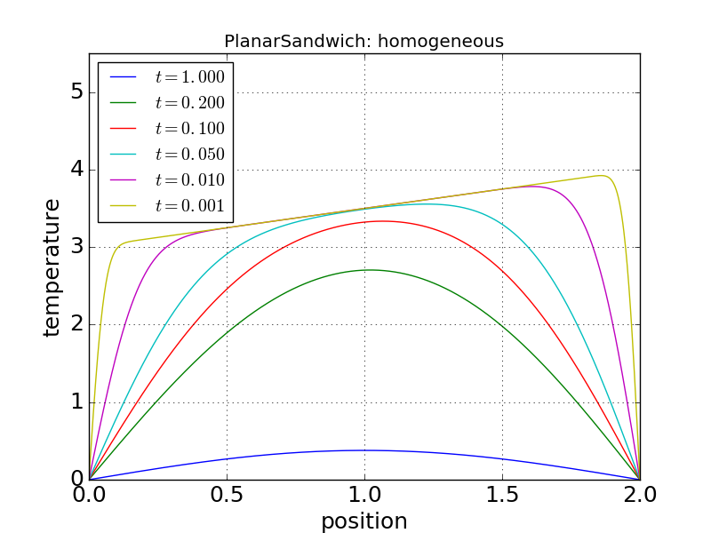
Figure 16: Temperature profiles for the homogeneous planar sandwich at times $t=1,0.2,0.1,0.01$, and $0.001$. The ExactPack class is PlanarSandwich(T1=0, T2=0, TA=3, TB=4, L=2, Nsum=1000), where we have set $\kappa=1$, $L=2$, $T_{\scriptscriptstyle\rm A}=3$, $T_{\rm\scriptscriptstyle B}=4$, with $T_{1}=T_{2}=0$. The boundary conditions $T_{1}=0$ and $T_{2}=0$ render the solution homogenous, while the linear initial condition $T_{0}(y)$ is specified by $T_{\scriptscriptstyle\rm A}$ and $T_{\rm\scriptscriptstyle B}$ via $T_{0}(y)=T_{\scriptscriptstyle\rm A}+\big{(}T_{\rm\scriptscriptstyle B}-T_{\scriptscriptstyle\rm A}\big{)}y/L$.

We close this discussion with a few comments on the general BCs for the class Rod1D. As an example let us consider the case

solver = Rod1D(alpha1=3, beta1=-1, gamma1=1,
               alpha2=1, beta2=2,  gamma2=1, L=2, TL=3, TR=3) ,

This corresponds to the BCs

$$3\,T(0,t)-\partial_{y}T(0,t) = 1$$ (51)

$$T(L,t)+2\,\partial_{y}T(L,t) = 1\ ,$$ (52)

and the solution is plotted in Fig. 17. Unlike the previous case, the IC is uniform, with $T_{\scriptscriptstyle\rm A}=T_{\rm\scriptscriptstyle B}=3$. The boundary conditions are mixed, and require numerically solving the equation $\mu\tan\mu=1$. In the next section, we perform rigorous convergence analyses for the half, hot, and warm planar sandwich variants. In fact, Rod1D is the parent class of PlanarSandwich and all other specialized planar sandwich classes, such as PlanarSandwichHalf and PlanarSandwichHot of the next two sections.

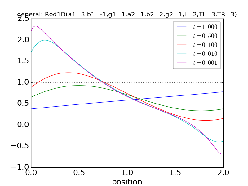
Figure 17: General boundary conditions: Rod1D(alpha1=3, beta1=-1, gamma1=1, alpha2=1, beta2=2, gamma2=1, TL=3, TR=3).

V.1 BC2: The Hot and Warm Planar Sandwiches

We now perform convergence analyses for several solutions of the boundary condition class BC2. These solutions are specified by the flux $F$ at the boundary points $y=0,L$, and the linear IC specified by $T_{\scriptscriptstyle\rm A}$ and $T_{\rm\scriptscriptstyle B}$. As shown in Ref. PlanarSandwichExactPackDoc , the corresponding exact solutions are of the form

$$T(y,t) = Fy+A_{0}+\sum_{n=1}^{\infty}A_{n}\,\cos(k_{n}y)\,e^{-\kappa\,k_{n}^{2}t}$$ (53)

$$k_{n} = \frac{n\pi}{L}\hskip 2.84544pt,\hskip 2.84544ptA_{0}=\frac{T_{\scriptscriptstyle\rm A}+T_{\rm\scriptscriptstyle B}}{2}\hskip 2.84544pt,\hskip 2.84544ptA_{n}=2\Big{(}T_{\scriptscriptstyle\rm A}-T_{\rm\scriptscriptstyle B}\Big{)}\frac{1-(-1)^{n}}{n^{2}\pi^{2}}\hskip 9.95863ptn\geq 1\ .$$ (54)

The hot planar sandwich of Ref. DMS is a special case in which the BC is $F=0$ and the IC is $T(y,0)=T_{0}$, and on physical grounds, the exact solution is given by the trivial solution

$$T(y,t)=T_{0}\ .$$ (55)

This solution is constant in time and uniform in space with value $T_{0}$. This also follow from (53) and (54) by setting $F_{\scriptscriptstyle\rm A}={\rm F}_{\rm\scriptscriptstyle B}=T_{0}$ and $F=0$. The hot planar sandwich is therefore given by $T_{\scriptscriptstyle\rm A}=T_{\rm\scriptscriptstyle B}=T_{0}$. In the analysis that follows, we take $T_{0}=3$, and consequently, $A_{0}=T_{0}$ and $A_{n}=0$ for $n\geq 1$, which reduces to the constant solution $T(y,t)=T_{0}$. This is illustrated in Fig. 18. This new variant of the planar sandwich can be instantiated by

solver = PlanarSandwichHot(F=0, TA=3, TB=3, L=2, Nsum=1000)  .

The heat flux $F$ on the boundaries has been set to zero, and a constant initial condition $T_{0}=3$, which has been specified $T_{0}=T_{\scriptscriptstyle\rm A}=T_{\rm\scriptscriptstyle B}=3$ in the ExactPack solution interface. On physical grounds, heat cannot escape from the material, and the temperature must remain constant, $T(y,t)=T_{0}$, as illustrated by the exact solution plotted in Fig. 18. The numerical results are give in Fig. 19 at time $t=0.1$, which indeed shows that the temperature remains constant. The lower panel of this Figure gives the convergence analysis. Note that the error is of order machine precision, and the points are scattered somewhat randomly, with a systematic linear increase at the higher precisions.

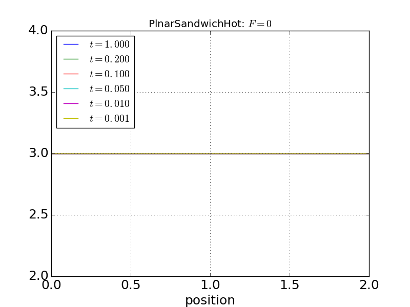
Figure 18: The hot planar sandwich in ExactPack: PlanarSandwichHot(F=0, TA=3, TB=3, L=2, Nsum=1000). Since the heat flux on the boundaries vanishes, heat cannot escape from the material, and the temperature must remain constant in time. The temperature profile has been plotted for the times $t=1,0.2,0.1,0.01$, and $0.001$, and is indeed constant.

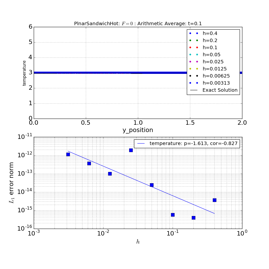
Figure 19: The hot planar sandwich. The parameter setting are the same as in Fig. 12, except the arithmetic average is used for multimaterial cells.

The next test problem will be called the warm planar sandwich. This problem allows heat to escape along the boundaries with flux $F=1$. The temperature profiles are illustrated in Fig. 20, and the numerical results in Figs. 21 – 24.

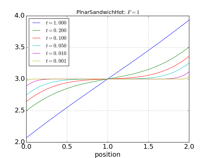
Figure 20: The warm planar sandwich in ExactPack: PlanarSandwichHot(F=1, TA=3, TB=3, L=2, Nsum=1000). The profiles are plotted for times $t=1,0.2,0.1,0.01$, and $0.001$. The heat flux at the boundaries is $F=1$, and we see that the temperature profile changes as heat flows out of the rod. In contrast to Fig. 19, when the heat flux is nonzero, heat is free to flow from the sandwich to the environment, and the temperature need not remain constant.

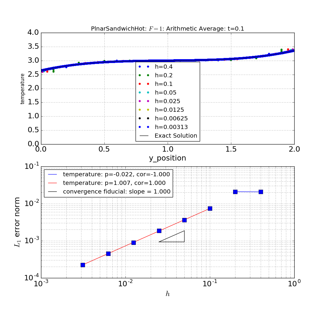
Figure 21: The parameter setting are the same as in Fig. 12, except the arithmetic average is used for multimaterial cells.

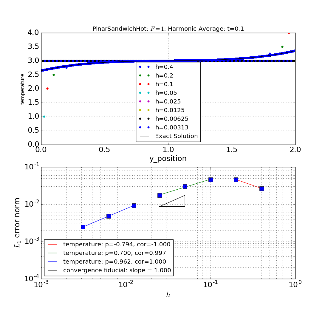
Figure 22: The parameter setting are the same as in Fig. 12, except the harmonic average is used for multimaterial cells.

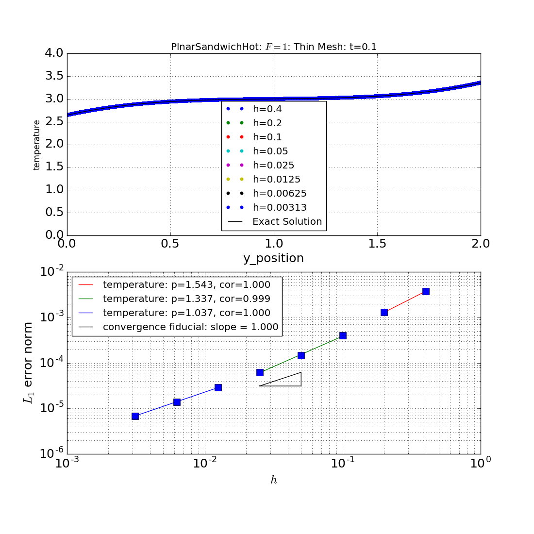
Figure 23: The parameter setting are the same as in Fig. 12, except the thin mesh option is used for multimaterial cells.

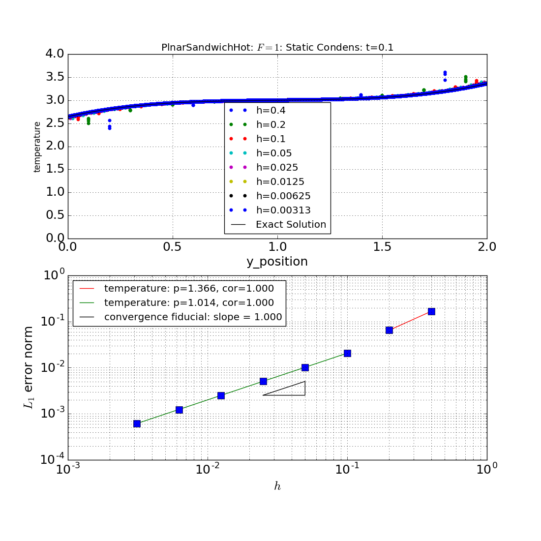
Figure 24: The parameter setting are the same as in Fig. 12, except the static condensation option is used for multimaterial cells.

V.2 The Half Planar Sandwich

The final variant we shall consider is given by choosing a vanishing heat flux on the upper boundary, $F_{2}=\partial_{y}T(L)=0$, and zero temperature on the lower boundary, $T_{1}=T(0)=0$. This is an example of boundary condition BC3, and we call the solution the half planar sandwich. For initial condition (34), Ref. PlanarSandwichExactPackDoc shows that the solution takes the form

$$T(y,t) = \sum_{n=0}^{\infty}B_{n}\,\sin(k_{n}y)\,e^{-\kappa\,k_{n}^{2}t}$$ (56)

$$k_{n} = \frac{(2n+1)\pi}{2L}\hskip 14.22636pt{\rm with}\hskip 14.22636ptB_{n}=\frac{4T_{\rm\scriptscriptstyle B}}{(2n+1)\pi}-\frac{8\big{(}T_{\rm\scriptscriptstyle B}-T_{\scriptscriptstyle\rm A}\big{)}}{(2n+1)^{2}\pi^{2}}\ .$$ (57)

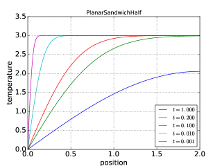
Figure 25: The half planar sandwich in ExactPack: PlanarSandwichHalf(T1=0, F2=0, TA=3, TB=3, L=2, Nsum=1000). The profiles are plotted for times $t=1,0.2,0.1,0.01$, and $0.001$. Note that the temperature profile vanishes on the bottom and the derivative of the temperature vanishes on the top.

Taking the initial condition $T_{0}=3$ ($T_{\scriptscriptstyle\rm A}=T_{\rm\scriptscriptstyle B}=3)$ gives Fig. 25, which is instantiated by solver = PlanarSandwichHalf(T1=0, F2=0, TA=3, TB=3, L=2, Nsum=1000)  .

If we had chosen $\partial_{y}T(0)=0$ and $T(L)=0$, as in BC4, then the plot would have been reflected about the midpoint of the rod, but is otherwise physically identical, as illustrated in Fig. 26. Figures 27 and 28 provide the solution plots and the convergence analyses for the arithmetic and harmonic averages of the half planar sandwich. As in the previous section, the top panel for the harmonic average in Fig. 28 exhibits near-zeros along the horizontal axis. Similarly, Figs. 29 and 30 illustrate the convergence analyses for the thin mesh and static condensation options for the half planar sandwich. The convergence plots for the half planar sandwich are qualitatively similar to those for the planar sandwich. In both cases, the arithmetic and harmonic averages are approximately $1^{\rm st}$ order, while thin mesh and static condensation start out at $2^{\rm nd}$ order and approach $1^{\rm st}$ order as the mesh is refined.

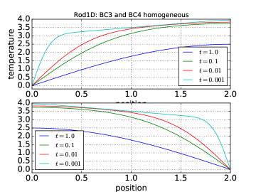
Figure 26: Note that BC3 and BC4 are physically equivalent, and are related by a parity inversion across the midpoint. The Figure uses $\kappa=1$, $L=2$, $T_{\scriptscriptstyle\rm A}=T_{\rm\scriptscriptstyle B}=3$. By symmetry principles, the two profiles are mirror images of one another. BC3 can be instantiated by Rod1D(alpha1=1, beta1=0, gamma1=1, alpha2=0, beta2=1, gamma2=0, TL=0, TR=0), and BC4 by Rod1D(alpha1=0, beta1=1, gamma1=0, alpha2=0, beta2=1, gamma2=F1, TL=0, TR=0). Note that $T_{\scriptscriptstyle\rm A}$ and $T_{\rm\scriptscriptstyle B}$ are interchanged between BC3 and BC4. The class Rod1D is the parent class of PlanarSandwich.

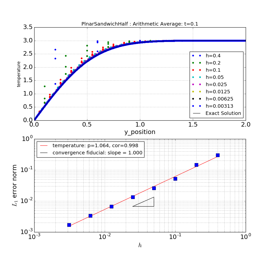
Figure 27: The parameter setting are the same as in Fig. 12.

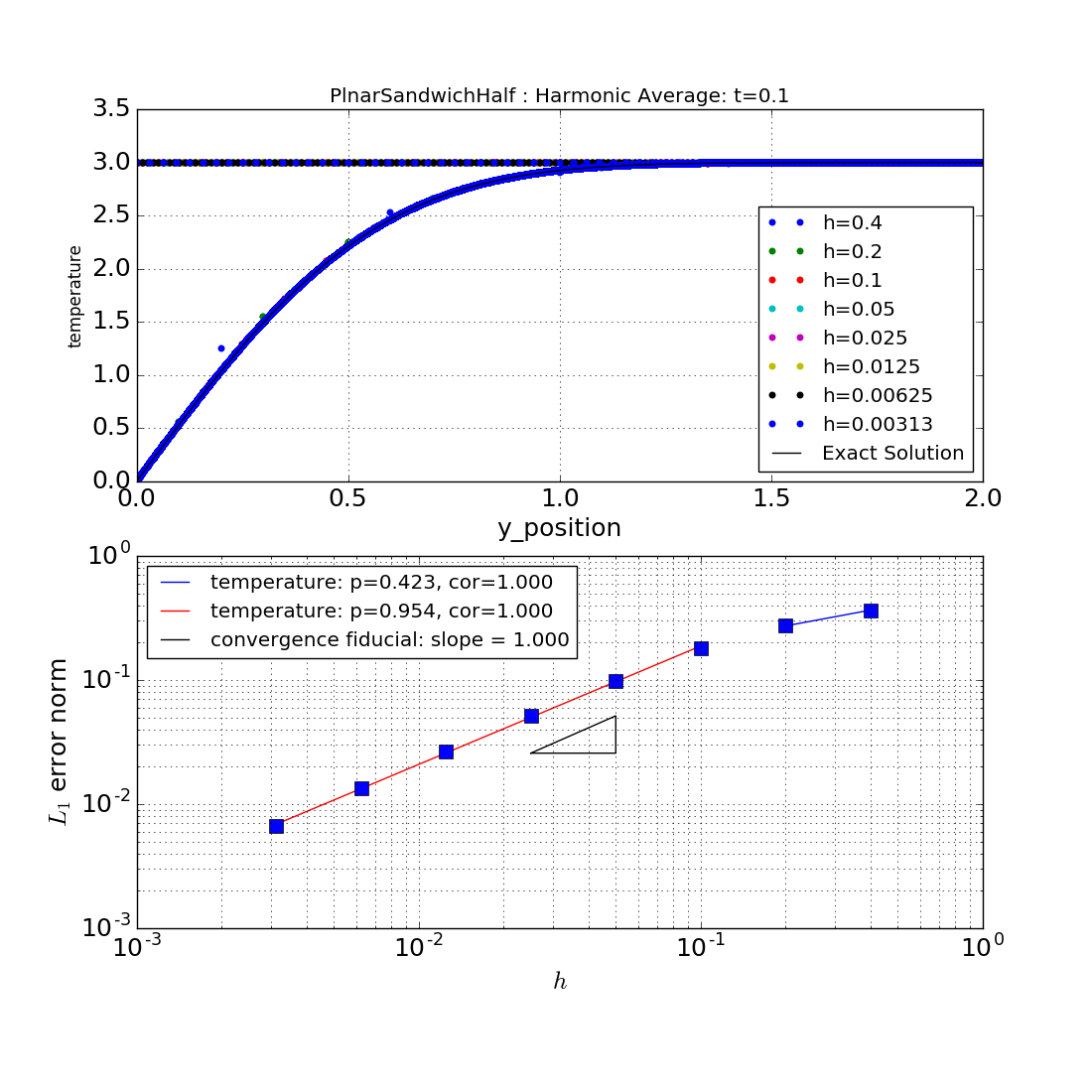
Figure 28: The parameter setting are the same as in Fig. 12, except the harmonic average is used for multimaterial cells.

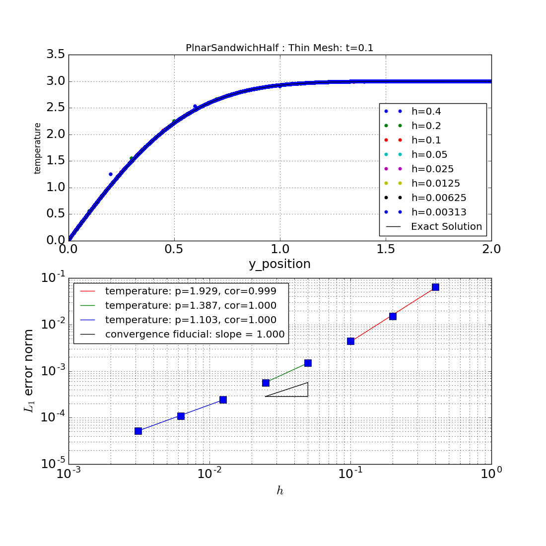
Figure 29: The parameter setting are the same as in Fig. 12, except the thin mesh option is used for multimaterial cells.

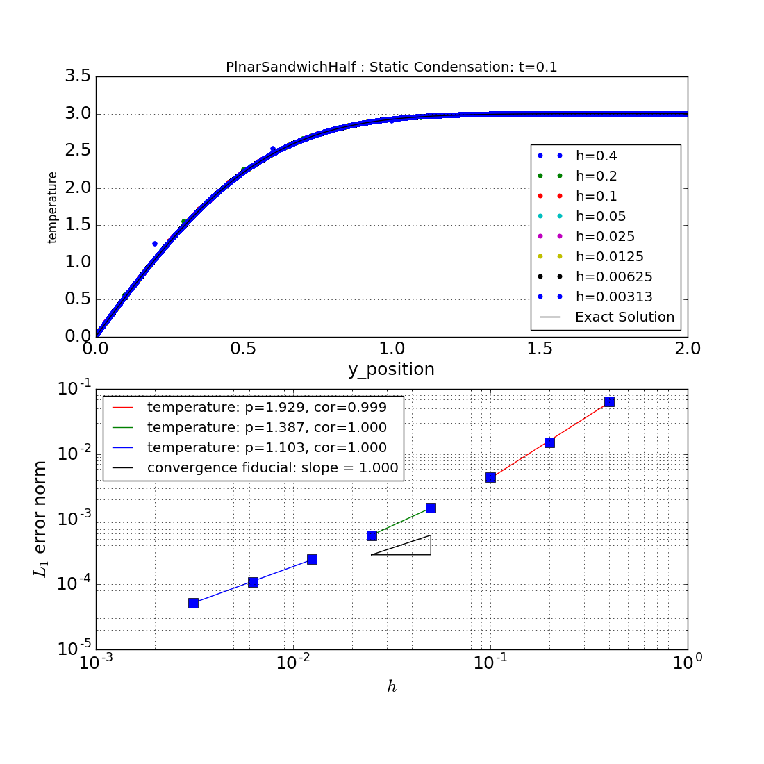
Figure 30: The parameter setting are the same as in Fig. 12, except the static condensation option is used for multimaterial cells.

VI Conclusions and Future Research

Two dimensional (2D) multimaterial heat diffusion can be a challenging numerical problem when the material boundaries are misaligned with the numerical grid. Even when the boundaries start out aligned, they typically become misaligned through hydrodynamic motion; therefore, it is important to perform rigorous verification analyses of the heat transport algorithms in any heat-conduction hydrocode. In this paper we perform convergence analyses for the four multimaterial heat flow algorithms in the multi-physics hydrodynamics code FLAG: (i) the arithmetic average, (ii) the harmonic average, (iii) thin mesh, and (iv) static condensation. To perform the analyses and to produce the corresponding convergence plots, we employ the code verification tool ExactPack. We concentrate on the 2D planar sandwich test problem, along with three generalizations called the half planar sandwich, the the hot planar sandwich, and the warm planar sandwich, all of which possess simple exact solutions. These test problems were designed to exhibit multimaterial cells along a fixed boundary, thereby exercising the multimaterial algorithms by the simplest means possible.

The geometry of the planar sandwich is illustrated in Fig. 1, which shows a square numerical grid overlaid on a rectangular physical geometry consisting of three parallel sandwich-like regions. The numerical grid partitions the physical geometry into a number of corresponding numerical cells, which need not align with the material regions. The outer two regions, called the bread of the sandwich, are composed of an insulating material with zero heat diffusion constant $\kappa_{1}=0$, while the inner region, called the meat of the sandwich, has diffusion coefficient $\kappa_{2}=\kappa>0$.

One of our primary results is that the arithmetic and harmonic averages converge at $1^{\rm st}$ order for all three variants of the planar sandwich. We also find that both the thin mesh and static condensation algorithms start out converging at $2^{\rm nd}$ order, but as the mesh is refined, the convergence rate levels off to $1^{\rm st}$ order. We conjecture that this is because the error in interface reconstruction algorithms becomes less precise at finer resolutions.

With more work, one can also construct an exact solution for the case in which $\kappa_{1}\neq 0$ in the bread of the sandwich RLSnotes , and these solutions might be an interesting avenue for future verification work. We are currently adding these solutions to ExactPack. We are also exploring Voronoi mesh simulations for the planar sandwich. Unlike the square mesh, Voronoi verification must be performed in 2D. This is because the Voronoi mesh does not align uniformly along $y=$constant, and one cannot use the 1D profiles for the exact solutions. Voronoi mesh verification is further complicated by the fact that the cells are not necessarily of equal area. Ref. Kamm99 explores the various choices of norm in such cases. We are adding a VTK reader to ExactPack, and this will greatly facilitate verification work with nonuniform meshes.

We also plan to study problems with more complicated geometry, such as the cylindrical sandwich. This test problem was proposed by Alan Dawes in Ref Dawes , and has been analyzed by Dawes, Shashkov, and Malone DMS . These authors did not perform convergence analyses, and they used a highly resolved “reference solution” rather than an exact solution, although the exact solution was presented in Appendix B of Ref. DMS . This test problem is much like the planar sandwich, except that the heat-conducting material is annular and lies in the first quadrant. The left most region is set to $T=1$ and the bottom region to $T=0$, and therefore heat moves clockwise along the annulus. See the left panel of Fig. 31. As illustrated by the right panel of Fig. 31, the square mesh will never align with the material boundary. Generalizations of the cylindrical sandwich exist much like those of Ref. PlanarSandwichExactPackDoc , and we plan to investigate these solutions as well.

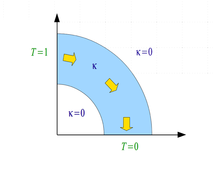
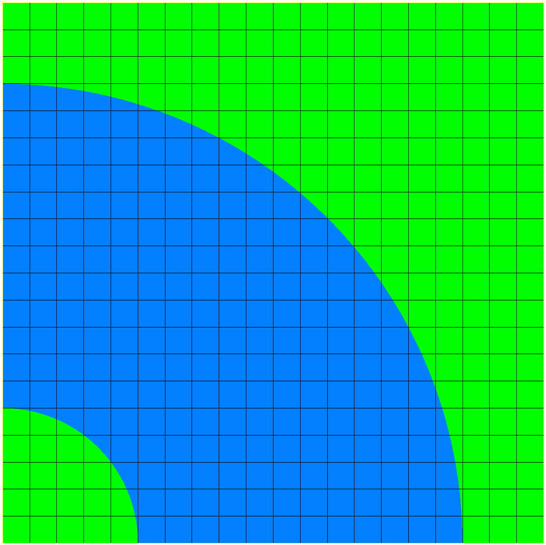
Figure 31: The cylindrical sandwich test problem. On the square grid, the multimaterial cells never align with the material boundary.

Appendix A Python script for the Planar Sandwich

import numpy as np
import matplotlib.pylab as plt

from exactpack.solvers.heat import PlanarSandwich

L = 2.0
x = np.linspace(0.0, L, 1000)
t1 = 1.0
t2 = 0.2
t3 = 0.1
t4 = 0.05
t5 = 0.01
t6 = 0.001

solver = PlanarSandwich(TB=1, TT=0, L=L, Nsum=1000)
soln1 = solver(x, t1)
soln2 = solver(x, t2)
soln3 = solver(x, t3)
soln4 = solver(x, t4)
soln5 = solver(x, t5)
soln6 = solver(x, t6)
soln1.plot(’temperature’, label=r’$t=1.000$’)
soln2.plot(’temperature’, label=r’$t=0.200$’)
soln3.plot(’temperature’, label=r’$t=0.100$’)
soln4.plot(’temperature’, label=r’$t=0.050$’)
soln5.plot(’temperature’, label=r’$t=0.010$’)
soln6.plot(’temperature’, label=r’$t=0.001$’)

plt.title(’PlanarSandwich’)
plt.ylabel(r’temperature’, fontsize=’18’)
plt.ylim(0,1)
plt.xlim(0,L)
plt.legend(loc=0)
plt.grid(True)
plt.savefig(’planar_sandwich.png’)
plt.show()

Appendix B ExactPack Script for Convergence Analysis

import numpy as np
import os.path
import glob
import matplotlib.pylab as plt

from exactpack.solvers.heat import PlanarSandwich
from exactpack.analysis import *
from lanl_readers.flag import FlagVarDump

#####################################################################
# problem parameters
L = 2.0
t = 0.1

# solver name
solver_name = ’PlanarSandwich’

# multimaterial alorithm
multimat = ’c1’ # arithmetic average
multimat_name = ’Arithmetic Average’

# study resolutions
res_study = [5, 10, 20, 40, 80, 160, 320, 640] # 8

# output tag
problem_out = ’planar_sandwich_{}_run16’.format(multimat)

# variable selection
variables = ’temperature’

# plot parameters
plot_params = {’temperature’: {’ymin’: 0, ’ymax’: 1, ’xmin’:0, ’xmax’: L,
  ’error_min’: 1.e-4, ’error_max’: 1.e-0, ’num’: [8], ’loc’: [1, 2, 1, 2]}
  }

# run dir and dump files
dumpfiles =/Users/bobs/mygit_repos/heat/runs/planar_sandwich/{}/res*/vardump/
  planar_sandwich_{}_VarDump.00000.1.000000E-01.zx’.format(multimat, multimat)

# create study_parameters
#####################################################################
study_parameters = [L/float(res) for res in res_study]

# creat solver
#####################################################################
solver = PlanarSandwich(TB=1, TT=0, L=L, Nsum=1000)

# study object
#####################################################################
print "*** plot solution and code data ..."

study = Study(sorted(glob.glob(dumpfiles)),
    reference=solver,
    study_parameters=study_parameters,
    time=t,
    reader=FlagVarDump(),
    abscissa=’y_position’
    )

#####################################################################
print "*** plot solution and code data ..."

xmin = plot_params[variable][’xmin’]
xmax = plot_params[variable][’xmax’]
ymin = plot_params[variable][’ymin’]
ymax = plot_params[variable][’ymax’]
loc = plot_params[variable][’loc’][0]

# plot solution profiles
plt.clf()
study.plot(’temperature’)
plt.xlim(xmin, xmax)
plt.ylim(ymin, ymax)
plt.ylabel(’$T$’)
plt.xlabel(’$y$’)
plt.title(r’{} : {}: t={}’.format(solver_name, multimat_name, t))
plt.legend(loc=loc)
plt.grid(True)
plt.savefig(problem_out+’_’+’temperature_soln.png’)
plt.show()

#####################################################################
print "*** convergence analysis ..."

error_max = plot_params[variable][’error_max’]
error_min = plot_params[variable][’error_min’]
loc = plot_params[variable][’loc’][1]
n0 = plot_params[variable][’num’][0]

domain = (0, L)
fiducials = {’temperature’: 1}
fit = RegressionConvergenceRate(study, norm=PointNorm(), domain=domain, fiducials=fiducials)
fit[:n0].plot_fit(’temperature’, "-", c=’r’)
fit.norms.plot(’temperature’, label=None, markersize=10)
fit.plot_fiducial(’temperature’)
plt.ylim(error_min, error_max)
plt.title(r’{} : {}: t={}’.format(solver_name, multimat_name, t))
plt.xlabel(r’$h$’)
plt.ylabel(r’$L_1$ error norm’)
plt.legend(loc=loc)
plt.savefig(problem_out+’_’+’temperature_conv.png’)
plt.show()

# plot on same axis
#####################################################################

xmin = plot_params[variable][’xmin’]
xmax = plot_params[variable][’xmax’]
ymin = plot_params[variable][’ymin’]
ymax = plot_params[variable][’ymax’]
error_max = plot_params[variable][’error_max’]
error_min = plot_params[variable][’error_min’]
n0 = plot_params[variable][’num’][0]
loc1 = plot_params[variable][’loc’][2]
loc2 = plot_params[variable][’loc’][3]

plt.figure(figsize=(11, 11))
ax = plt.subplot(211)
study.plot(’temperature’)
plt.xlim(xmin, xmax)
plt.ylim(ymin, ymax)
plt.ylabel(’$T$’)
plt.xlabel(’$y$’)
plt.title(r’{} : {}: t={}’.format(solver_name, multimat_name, t))
plt.legend(loc=loc1)
plt.grid(True)

ax = plt.subplot(212)
domain = (0, L)
fiducials = {’temperature’: 1}
fit = RegressionConvergenceRate(study, norm=PointNorm(),
  domain=domain, fiducials=fiducials)
fit[:n0].plot_fit(’temperature’, "-", c=’r’)
fit.norms.plot(’temperature’, label=None, markersize=10)
fit.plot_fiducial(’temperature’)
plt.ylim(error_min, error_max)
plt.xlabel(r’$h$’)
plt.ylabel(r’$L_1$ error norm’)
plt.legend(loc=loc2)
plt.savefig(problem_out+’_’+’temperature_soln_conv.png’)
plt.show()

Appendix C Solution to the Planar Sandwich

In this section we find the general solution to the heat equation (27)–(30). The differential equation (DE), the boundary conditions (BCs), and the initial condition (IC) are reproduced here for convenience,

$${\rm DE}:\hskip 106.12865pt\frac{\partial T(y,t)}{\partial t} = \kappa\,\frac{\partial^{2}T(y,t)}{\partial y^{2}}\hskip 34.14322pt0<y<L~{}{\rm and}~{}t>0$$ (58)

$${\rm BCs}:\hskip 33.0053pt\alpha_{1}T(0,t)+\beta_{1}\partial_{y}T(0,t) = \gamma_{1}\hskip 79.6678ptt>0~{},~{}y=0,L$$ (59)

$$\alpha_{2}T(L,t)+\beta_{2}\partial_{y}T(L,t) = \gamma_{2}$$ (60)

$${\rm IC}:\hskip 115.23373ptT(y,0) = T_{0}(y)\hskip 62.59596pt0<y<L~{},~{}t=0\ .$$ (61)

The solution is obtained by solving two independent problems: (i) finding a specific static nonhomogeneous solution $\bar{T}(y)$ and (ii) finding the general homogeneous solution $\tilde{T}(y,t)$ satisfying the initial condition

$$\tilde{T}(y,0)=T_{0}(y)-\bar{T}(y)\ .$$ (62)

The homogeneous solution $\tilde{T}(y,t)$ can be represented as a Fourier series. Note that $\bar{T}$ depends upon the BCs, while $\tilde{T}$ depends upon the IC and the BCs. Once $\bar{T}$ and $\tilde{T}$ have been found, the general solution is given by

$$T(y,t)=\bar{T}(y)+\tilde{T}(y,t)\ .$$ (63)

Note that $T(y,t)$ satisfies the initial condition $T(y,0)=T_{0}(y)$, and is the unique solution because of the maximum principle.

C.1 The Static Nonhomogeneous Problem

Because of its simplicity, we first turn to finding the static nonhomogeneous solution $\bar{T}(y)$. In the static limit, the differential equation (58) and boundary conditions (60) reduce to

$$\frac{\partial^{2}\bar{T}(y)}{\partial x^{2}} = 0$$ (64)

$$\alpha_{1}\bar{T}(0)+\beta_{1}\bar{T}^{\prime}(0) = \gamma_{1}$$ (65)

$$\alpha_{2}\bar{T}(L)+\beta_{2}\bar{T}^{\prime}(L) = \gamma_{2}\ .$$ (66)

The initial condition (61) of the full time dependent problem can be ignored since we are only interested in static solutions. The general solution to (64) is trivial, and takes the form

$$\bar{T}(y)=a+by\ .$$ (67)

For Dirichlet boundary conditions, we must specify the temperature values $T_{1}$ and $T_{2}$ at the endpoints, thereby giving the nonhomogenous static solution

$$\bar{T}(y) = T_{1}+\frac{T_{2}-T_{1}}{L}\,y\ .$$ (68)

The coefficients $a$ and $b$, or equivalently $T_{1}$ and $T_{2}$, are determined by $\bar{T}(0)=a=T_{1}$ and $\bar{T}(L)=a+bL=T_{2}$. For a Neumann BC specified by flux $F_{i}$, we can always rewrite the corresponding homogeneous solution in the form (68) by the defining temperature $T_{i}=F_{i}L$, where we can take $i=1,2$. The solution to

The BCs (65) and (66) can be written as a linear equation in terms of $a$ and $b$,

$$\left(\begin{array}[]{cc}\alpha_{1}&\beta_{1}\\ \alpha_{2}&~{}\beta_{2}+\alpha_{2}L\end{array}\right)\left(\begin{array}[]{c}a\\ b\end{array}\right)=\left(\begin{array}[]{c}\gamma_{1}\\ \gamma_{2}\end{array}\right)\ .$$ (75)

Upon solving the system of equations we find

$$a = \frac{\beta_{2}\gamma_{1}-\beta_{1}\gamma_{2}+L\alpha_{2}\gamma_{1}}{\alpha_{1}\beta_{2}-\alpha_{2}\beta_{1}+L\alpha_{1}\alpha_{2}}$$ (76)

$$b = \frac{\alpha_{1}\gamma_{2}-\alpha_{2}\gamma_{1}}{\alpha_{1}\beta_{2}-\alpha_{2}\beta_{1}+L\alpha_{1}\alpha_{2}}\ ,$$ (77)

or in terms of temperature parameters $T_{1}=a$ and $T_{2}=a+bL$,

$$T_{1} = \frac{\beta_{2}\gamma_{1}-\beta_{1}\gamma_{2}+L\alpha_{2}\gamma_{1}}{\alpha_{1}\beta_{2}-\alpha_{2}\beta_{1}+L\alpha_{1}\alpha_{2}}$$ (78)

$$T_{2} = \frac{\beta_{2}\gamma_{1}-\beta_{1}\gamma_{2}+L\alpha_{1}\gamma_{2}}{\alpha_{1}\beta_{2}-\alpha_{2}\beta_{1}+L\alpha_{1}\alpha_{2}}\ .$$ (79)

Note that the determinant of the linear equations vanishes for BC2, and we must handle this case separately. We can also express the BCs in terms of the fluxes

$$F_{1} = T_{1}/L$$ (80)

$$F_{2} = T_{2}/L\$$ (81)

by writing

$$\bar{T}(y) = T_{1}+(F_{1}-F_{2})y\ .$$ (82)

We can also express $\bar{T}(y)$ by combinations of temperature and flux.

Special Cases of the Static Problem

a. BC1

Let us consider the simple Dirichlet boundary conditions (39) and (40),

$$\bar{T}(0) = T_{1}$$ (83)

$$\bar{T}(L) = T_{2}\ ,$$ (84)

which gives the solution

$$\bar{T}(y) = T_{1}+\frac{T_{2}-T_{1}}{L}\,y\ .$$ (85)

The temperature coefficients are given by

$$T_{1} = \frac{\gamma_{1}}{\alpha_{1}}$$ (86)

$$T_{2} = \frac{\gamma_{2}}{\alpha_{2}}\ ,$$ (87)

which follows from Eqs. (65) and (66), or equivalently from Eqs. (78) and (79) with $\beta_{1}=\beta_{2}=0$. Similarly, the coefficients in (67) are $a=T_{1}$ and $b=(T_{2}-T_{1})/L$.

b. BC2

Let us now find the nonhomogeneous equilibrium solution for the Neumann boundary conditions (41) and (42),

$$\partial_{y}\bar{T}(0) = F_{1}$$ (88)

$$\partial_{y}\bar{T}(L) = F_{2}\ ,$$ (89)

where $F_{1}$ and $F_{2}$ are the heat fluxes at $y=0$ and $y=L$, respectively. The fluxes and are related to the boundary condition parameters in (65) and (66) by $F_{1}=\gamma_{1}/\beta_{1}$ and $F_{2}=\gamma_{2}/\beta_{2}$ with $\alpha_{1}=\alpha_{2}=0$. As before, the general solution is $\bar{T}(y)=a+by$, and we see that $\bar{T}^{\prime}(y)=b$ is independent of $y$. In other words, the heat flux at either end of the rod must be identical, $F_{1}=b=F_{2}$. In fact, this result follows from energy conservation, since, in static equilibrium, the heat flowing into the rod must be equal the heat flowing out of the rod. More correctly, we should therefore start with the boundary conditions

$$\partial_{y}\bar{T}(0) = F$$ (90)

$$\partial_{y}\bar{T}(L) = F\ ,$$ (91)

where

$$F=\frac{\gamma_{1}}{\beta_{1}}=\frac{\gamma_{2}}{\beta_{2}}\ .$$ (92)

The value of the constant term $a$ is not uniquely determined in this case; however, we are free to set it to zero, or to combine it with the constant $A_{0}$ term of $\tilde{T}(y,t)$, thereby giving

$$\bar{T}(y)=Fy\ .$$ (93)

There is nothing wrong with setting $a=0$, since we only need to find one nonhomogeneous solution, and (93) fits the bill. We can write this solution in the form (68), with

$$T_{1} = 0$$ (94)

$$T_{2} = FL\ .$$ (95)

c. BC3

We now consider the mixed Dirichlet and Neumann boundary conditions (43) and (44),

$$\bar{T}(0) = T_{1}$$ (96)

$$\partial_{y}\bar{T}(L) = F_{2}\ .$$ (97)

We can express the solution (68) in terms of the temperature $T_{1}$, and the effective temperature

$$T_{2} = T_{1}+F_{2}L=\frac{\gamma_{1}}{\alpha_{1}}+\frac{\gamma_{2}L}{\beta_{2}}\ ,$$ (98)

and the solution takes the form

$$\bar{T}(y)=T_{1}+F_{2}y\ .$$ (99)

d. BC4

The boundary conditions are (45) and (46),

$$\partial_{y}\bar{T}(0) = F_{1}$$ (100)

$$\bar{T}(L) = T_{2}\ ,$$ (101)

and the solution (68) can be written The solution takes the form

$$\bar{T}(y)=(T_{2}-F_{1}L)+F_{1}y\ .$$ (102)

We can define an effective temperature

$$T_{1} = T_{2}-F_{1}L=\frac{\gamma_{2}}{\alpha_{2}}-\frac{\gamma_{1}L}{\beta_{1}}\ ,$$ (103)

C.2 The General Homogeneous Problem

Now that we have constructed the static nonhomogenous solution $\bar{T}(y)$ appropriate to the choice of boundary conditions, we turn to the slightly more involved task of finding the general homogeneous solution $\tilde{T}(y,t)$. This is equivalent to solving a discrete eigenvalue problem, albeit in an infinite number of dimensions. We then construct the solution $\tilde{T}(y,t)$ as a weighted sum over the normal modes, where the weights are determined by the choice of BCs and the IC. The special cases BC1, BC2, BC3, and BC4 are particularly simple. The homogeneous equations of motion, for which $\gamma_{1}=0$ and $\gamma_{2}=0$, take the form

$${\rm DE}:\hskip 106.12865pt\frac{\partial\tilde{T}(y,t)}{\partial t} = \kappa\,\frac{\partial^{2}\tilde{T}(y,t)}{\partial y^{2}}\hskip 34.14322pt0<y<L~{}{\rm and}~{}t>0$$ (104)

$${\rm BC}:\hskip 33.0053pt\alpha_{1}\tilde{T}(0,t)+\beta_{1}\partial_{y}\tilde{T}(0,t) = 0\hskip 83.93553ptt>0$$ (105)

$$\alpha_{2}\tilde{T}(L,t)+\beta_{2}\partial_{y}\tilde{T}(L,t) = 0$$

$${\rm IC}:\hskip 115.23373pt\tilde{T}(y,0) = T_{0}(y)\hskip 62.59596pt0<y<L\ .$$ (106)

As we have discussed, we shall focus on the linear initial condition

$$T_{0}(y)=T_{\scriptscriptstyle\rm A}+\frac{T_{\rm\scriptscriptstyle B}-T_{\scriptscriptstyle\rm A}}{L}\,y\hskip 128.0374pt0<y<L\ ,$$ (107)

although, more generally, any continuous function $T_{0}(y)$ will produce a solution.

The solution technique is by separation of variables, for which we assume the solution to be a product of independent functions of $y$ and $t$,

$$\tilde{T}(y,t)=Y(y)\,U(t)\ .$$ (108)

Substituting this Ansatz into the heat equation gives

$$\frac{dU(t)}{dt}\,Y(y)=\kappa\,U(t)\,\frac{d^{2}Y(y)}{dy^{2}}\ ,$$ (109)

or

$$\frac{1}{\kappa}\,\frac{U^{\prime}(t)}{U(t)}=\frac{Y^{\prime\prime}(y)}{Y(y)}={\rm const}\equiv-k^{2}\ ,$$ (110)

where we have chosen the constant negative value $-k^{2}$, and we have expressed the derivatives of $U(t)$ and $Y(y)$ by primes. As usual in the separation of variables technique, when two functions of different variables are equated, they must be equal to a constant, independent of $y$ and $t$. The variable $U(t)$ satisfies

$$U^{\prime}(t)=-\kappa\,k^{2}\,U(t)\ ,$$ (111)

which has the solution

$$U_{k}(t) = U_{0}\,e^{-\kappa\,k^{2}t}\ .$$ (112)

We have introduced a $k$-subscript in $U_{k}$ to indicate that the solution depends upon the value of $k$. Without loss of generality we set $U_{0}=1$. We now find that the equation for $Y$ reduces to

$$Y^{\prime\prime}(y)+k^{2}Y(y) = 0$$ (113)

$$\alpha_{1}Y(0)+\beta_{1}Y^{\prime}(0) = 0$$ (114)

$$\alpha_{2}Y(L)+\beta_{2}Y^{\prime}(L) = 0\ .$$

The general solution to (113) is

$$Y_{k}(y)=A_{k}\cos ky+B_{k}\sin ky\ .$$ (115)

When the BCs are applied, the modes $Y_{k}$ will be orthogonal,

$$\int_{0}^{L}dx\,Y_{k}(y)Y_{k^{\prime}}(y)=N_{k}\,\delta_{kk^{\prime}}\ .$$ (116)

It is instructive to prove the orthogonality relation (116) directly from the differential equation. Given two solutions $Y_{k}$ and $Y_{k^{\prime}}$ to (113), we can write the two alternative forms,

$$Y_{k^{\prime}}\Big{[}Y_{k}^{\prime\prime}+k^{2}Y_{k}\Big{]} = 0$$ (117)

$$Y_{k}\Big{[}Y_{k^{\prime}}^{\prime\prime}+k^{\prime\,2}Y_{k^{\prime}}\Big{]} = 0\ .$$ (118)

These forms differ only in the interchange of $k$ and $k^{\prime}$. Upon subtracting these equations, and then integrating over space, we find

$$(k^{2}-k^{\prime\,2})\int_{0}^{L}\!dy\,Y_{k}\,Y_{k^{\prime}} = \int_{0}^{L}\!dy\,\Big{[}Y_{k}Y_{k^{\prime}}^{\prime\prime}-Y_{k^{\prime}}Y_{k}^{\prime\prime}\Big{]}$$

$$= \int_{0}^{L}\!dy\,\Big{[}\frac{d}{dy}\,\Big{(}Y_{k}Y_{k^{\prime}}^{\prime}\Big{)}-Y_{k}^{\prime}Y_{k^{\prime}}^{\prime}-\frac{d}{dy}\Big{(}Y_{k^{\prime}}Y_{k}^{\prime}\Big{)}+Y_{k^{\prime}}^{\prime}Y_{k}^{\prime}\Big{]}$$

$$= \int_{0}^{L}\!dy\,\frac{d}{dy}\,\Big{(}Y_{k}Y_{k^{\prime}}^{\prime}-Y_{k^{\prime}}Y_{k}^{\prime}\Big{)}$$ (120)

$$= \Big{(}Y_{k}Y_{k^{\prime}}^{\prime}-Y_{k^{\prime}}Y_{k}^{\prime}\Big{)}\Big{|}_{0}^{L}=0\ ,$$ (121)

where each contribution from $y=0$ and $y=L$ vanishes separately because of their respective boundary conditions. We therefore arrive at

$$(k^{2}-k^{\prime\,2})\int_{0}^{L}\!dy\,Y_{k}\,Y_{k^{\prime}}=0\ .$$ (122)

Provided $k\neq k^{\prime}$, we can divide (122) by $k^{2}-k^{\prime\,2}$ to obtain

$$\int_{0}^{L}\!dy\,Y_{k}(y)\,Y_{k^{\prime}}(y) = 0~{}~{}~{}{\rm when}~{}k\neq k^{\prime}\ .$$ (123)

When $k=k^{\prime}$, (122) gives no constraint on the normalization integral. However, since the differential equation is linear, and since the BCs are homogeneous and linear, we are free to normalize $Y_{k}$ over $[0,L]$ such that $\int dy\,Y_{k}^{2}=N_{k}$ for any convenient choice of $N_{k}$.

We now express the general time dependent solution as a sum over all modes,

$$\tilde{T}(y,t)={\sum}_{k}D_{k}\,Y_{k}(y)\,e^{-\kappa\,k^{2}t}\ .$$ (124)

The coefficients $D_{k}$ themselves are chosen so that the initial condition is satisfied,

$$\tilde{T}(y,0) = {\sum}_{k}D_{k}Y_{k}(y)=T_{0}(y)-\bar{T}(y)$$ (125)

$$~{}~{}~{}\Rightarrow~{}~{}~{}D_{k} = \frac{1}{N_{k}}\int_{0}^{L}\!dy\,\Big{[}T_{0}(y)-\bar{T}(y)\Big{]}\,Y_{k}(y)\ .$$ (126)

Substituting (107) and (68) into (125) gives

$$\tilde{T}(y,0) = T_{0}(y)-\bar{T}(y)$$ (127)

$$= T_{a}+\frac{T_{b}-T_{a}}{L}\,y\ ,$$ (128)

with

$$T_{a} = T_{\scriptscriptstyle\rm A}-T_{1}$$ (129)

$$T_{b} = T_{\rm\scriptscriptstyle B}-T_{2}\ .$$ (130)

Therefore, the coefficients $D_{k}=D_{k}(T_{a},T_{b})$ are functions of $T_{a}$ and $T_{b}$.

Special Cases of the Homogeneous Problem

a. BC1

In the first case we hold the temperature fixed to zero at both ends of the rod,

$$\tilde{T}(0,t) = 0$$ (131)

$$\tilde{T}(L,t) = 0\ .$$ (132)

The general solution $Y_{k}(y)\!=\!A_{k}\cos ky+B_{k}\sin ky$ reduces to $Y_{k}(y)=B_{k}\sin ky$ under (131), while (132) restricts the wave numbers to satisfy $\sin kL=0$, i.e. $k=k_{n}=n\pi/L$ for $n=1,2,3,\cdots$. Note that $n=0$ does not contribute, since this gives the trivial vanishing solution. It is convenient to label the modes by the mode number $n$ rather than the wave number $k_{n}$, so that the homogeneous solution takes the form

$$\tilde{T}(y,t) = \sum_{n=1}^{\infty}B_{n}\,Y_{n}(y)\,e^{-\kappa\,k_{n}^{2}t}$$ (133)

$$Y_{n}(y) = \sin k_{n}y$$ (134)

$$k_{n} = \frac{n\pi}{L}\hskip 28.45274ptn=1,2,3,\cdots\ .$$ (135)

The tilde over the temperature is meant to explicitly remind us that this is the general homogeneous solution. The orthogonality condition on the modes $Y_{n}$ can be checked by a simple integration,

$$\int_{0}^{L}dy\,Y_{n}(y)Y_{m}(y) = \frac{L}{2}\,\delta_{nm}\ .$$ (136)

For an initial condition $\tilde{T}(y,0)=T_{0}(y)$, we can calculate the corresponding coefficients in the Fourier sum,

$$B_{n}=\frac{2}{L}\int_{0}^{L}dy\,T_{0}(y)\sin k_{n}y\ .$$ (137)

For the linear initial condition (107), a simple calculation gives

$$B_{n} = 2T_{\scriptscriptstyle\rm A}\,\frac{1-(-1)^{n}}{n\pi}+2(T_{\scriptscriptstyle\rm A}-T_{\rm\scriptscriptstyle B})\,\frac{(-1)^{n}}{n\pi}$$ (138)

$$= \frac{2T_{\scriptscriptstyle\rm A}-2T_{\rm\scriptscriptstyle B}(-1)^{n}}{n\pi}\ .$$ (139)

b. BC2

The second special boundary condition that we consider sets the heat flux at both ends of the rod to zero,

$$\partial_{y}\tilde{T}(0,t) = 0$$ (140)

$$\partial_{y}\tilde{T}(L,t) = 0\ .$$ (141)

This is the hot planar sandwich. The general solution $Y_{k}(y)\!=\!A_{k}\cos ky+B_{k}\sin ky$ reduces to $Y_{k}(y)=A_{k}\cos ky$ under (140) , while (141) restricts the wave numbers to $k\sin kL=0$, so that $k=k_{n}=n\pi/L$ for $n=0,1,2\cdots$. In this case, the $n=0$ mode is permitted (and indeed essential), and the solution can be written

$$\tilde{T}(y,t) = \frac{A_{0}}{2}+\sum_{n=1}^{\infty}A_{n}\,Y_{n}(y)\,e^{-\kappa\,k_{n}^{2}t}$$ (142)

$$Y_{n}(y) = \cos k_{n}y$$ (143)

$$k_{n} = \frac{n\pi}{L}\hskip 28.45274ptn=0,1,2,\cdots\ ,$$ (144)

where a conventional factor of $1/2$ has been inserted in the $A_{0}$ term. This is because of the difference in normalization between $n=0$ and $n\neq 0$,

$$\int_{0}^{L}dy\,Y_{0}^{2}(y) = L$$ (145)

$$\int_{0}^{L}dy\,Y_{n}^{2}(y) = \frac{L}{2}~{}~{}~{}~{}n\neq 0\ .$$ (146)

Given the initial condition $\tilde{T}(y,0)=T_{0}(y)$, the Fourier modes become

$$A_{n}=\frac{2}{L}\,\int_{0}^{L}dy\,T_{0}(y)\cos k_{n}y$$ (147)

for $n=0,1,2\cdots$. This holds for all values of $n$, including $n=0$. This is why we used the factor of 1/2 in the $A_{0}$ term of (142). For simplicity, we will take the linear initial condition (107) for $T_{0}(y)$, in which case, (147) gives the coefficients

$$\frac{A_{0}}{2} = \frac{1}{2}\Big{(}T_{\scriptscriptstyle\rm A}+T_{\rm\scriptscriptstyle B}\Big{)}$$ (148)

$$A_{n} = 2\,\Big{(}T_{\scriptscriptstyle\rm A}-T_{\rm\scriptscriptstyle B}\Big{)}\,\frac{1-(-1)^{n}}{n^{2}\pi^{2}}\ .$$ (149)

For pedagogical purposes, let us work through the algebra for the $A_{n}$ coefficients, doing the $n=0$ case first:

$$\frac{A_{0}}{2} = \frac{1}{L}\int_{0}^{L}\,T_{0}(y)=\frac{1}{L}\int_{0}^{L}\,\left[T_{\scriptscriptstyle\rm A}+\frac{T_{\rm\scriptscriptstyle B}-T_{\scriptscriptstyle\rm A}}{L}\,y\right]$$ (150)

$$= T_{\scriptstyle L}+\left[\frac{T_{\rm\scriptscriptstyle B}-T_{\scriptscriptstyle\rm A}}{2}\right]=\frac{1}{2}\left[T_{\rm\scriptscriptstyle B}+T_{\scriptscriptstyle\rm A}\right]\ .$$ (151)

Next, taking $n\neq 0$, we find:

$$A_{n} = \frac{2}{L}\int_{0}^{L}dy\,T_{0}(y)\cos k_{n}y$$ (152)

$$= \frac{2}{L}\int_{0}^{L}dy\,\left[T_{\scriptscriptstyle\rm A}+\frac{T_{\rm\scriptscriptstyle B}-T_{\scriptscriptstyle\rm A}}{L}\,y\right]\cos k_{n}y$$ (153)

$$= T_{\scriptscriptstyle\rm A}\,\frac{2}{L}\int_{0}^{L}dy\,\cos k_{n}y+\Big{(}T_{\rm\scriptscriptstyle B}-T_{\scriptscriptstyle\rm A}\Big{)}\frac{2}{L^{2}}\int_{0}^{L}dy\,y\,\cos k_{n}y\ .$$ (154)

The first term integrates to zero since

$$\frac{2}{L}\int_{0}^{L}dy\,\cos k_{n}y = \frac{2}{L}\,\sin k_{n}y\Big{|}_{y=0}^{y=L}=0\ ,$$ (155)

and the second term gives

$$\frac{2}{L^{2}}\int_{0}^{L}dy\,y\,\cos k_{n}y = \frac{2}{L^{2}}\left[\frac{\cos k_{n}y}{k_{n}^{2}}+\frac{y\sin k_{n}y}{k_{n}}\right]_{y=0}^{y=L}$$ (156)

$$= \frac{2}{L^{2}}\,\frac{L^{2}}{n^{2}\pi^{2}}\,\Big{[}\cos k_{n}L-1\Big{]}=2\,\frac{(-1)^{n}-1}{n^{2}\pi^{2}}\ ,$$ (157)

which leads to (149).

c. BC3

The next specialized boundary condition is

$$\tilde{T}(0,t) = 0$$ (158)

$$\partial_{y}\tilde{T}(L,t) = 0\ .$$ (159)

This is the half planar sandwich. The general solution $Y_{k}(y)\!=\!A_{k}\cos ky+B_{k}\sin ky$ under (158) reduces to $Y_{k}(y)=B_{k}\sin ky$, while (159) restricts the wave numbers to $k\cos kL=0$, so that $k=k_{n}=(2n+1)\pi/2L$ for $n=0,1,2\cdots$. The general homogeneous solution is therefore

$$\tilde{T}(y,t) = \sum_{n=0}^{\infty}B_{n}\,Y_{n}(y)\,e^{-\kappa\,k_{n}^{2}t}$$ (160)

$$Y_{n}(y) = \sin k_{n}y$$ (161)

$$k_{n} = \frac{(2n+1)\pi}{2L}\hskip 28.45274ptn=0,1,2,\cdots\ .$$ (162)

The initial condition $\tilde{T}(y,0)=T_{0}(y)$ gives the Fourier modes

$$B_{n}=\frac{2}{L}\,\int_{0}^{L}dy\,T_{0}(y)\sin k_{n}y\ ,$$ (163)

and, upon taking the linear initial condition (34), we find

$$B_{n} = \frac{4T_{\scriptscriptstyle\rm A}}{(2n+1)\pi}+4\big{(}T_{\rm\scriptscriptstyle B}-T_{\scriptscriptstyle\rm A}\big{)}\left[\frac{1}{(2n+1)\pi}-\frac{2}{(2n+1)^{2}\pi^{2}}\right]$$ (164)

$$= \frac{4T_{\rm\scriptscriptstyle B}}{(2n+1)\pi}-\frac{8\big{(}T_{\rm\scriptscriptstyle B}-T_{\scriptscriptstyle\rm A}\big{)}}{(2n+1)^{2}\pi^{2}}\ .$$ (165)

d. BC4

The last special case is the boundary condition

$$\partial_{y}\tilde{T}(0,t) = 0$$ (166)

$$\tilde{T}(L,t) = 0\ .$$ (167)

The general solution $Y_{k}(y)\!=\!A_{k}\cos ky+B_{k}\sin ky$ reduces to $Y_{k}(y)=A_{k}\cos ky$ under (166), while (167) restricts the wave numbers to $\cos kL=0$, i.e. $k=k_{n}=(2n+1)\pi/2L$ for $n=0,1,2\cdots$, which gives rise to the homogeneous solution

$$\tilde{T}(y,t) = \sum_{n=0}^{\infty}A_{n}\,Y_{n}(y)\,e^{-\kappa\,k_{n}^{2}t}$$ (168)

$$Y_{n}(y) = \cos k_{n}y$$ (169)

$$k_{n} = \frac{(2n+1)\pi}{2L}\hskip 28.45274ptn=0,1,2,\cdots\ .$$ (170)

Similar to (163), the mode coefficient is

$$A_{n}=\frac{2}{L}\,\int_{0}^{L}dy\,T_{0}(y)\cos k_{n}y\ ,$$ (171)

and, upon taking the linear initial condition (107), we find

$$A_{n} = 4T_{\scriptscriptstyle\rm A}\,\frac{(-1)^{n}}{(2n+1)\pi}-8\Big{(}T_{\rm\scriptscriptstyle B}-T_{\scriptscriptstyle\rm A}\Big{)}\,\frac{1-(-1)^{n}}{(2n+1)^{2}\,\pi^{2}}\ .$$ (172)

Note that BC3 and BC4 are in fact equivalent, and represent a rod that has been flipped from left to right about its center, as illustrated in Fig. 26.

General Boundary Conditions

We now turn to the general form of the boundary conditions, which, expressed in terms of $Y$, take the form

$$\alpha_{1}Y_{k}(0)+\beta_{1}Y_{k}^{\prime}(0) = 0$$ (173)

$$\alpha_{2}Y_{k}(L)+\beta_{2}Y_{k}^{\prime}(L) = 0\ .$$ (174)

The solution and its derivative are

$$Y_{k}(y) = A\cos ky+B\sin ky$$ (175)

$$Y_{k}^{\prime}(y) = -Ak\sin ky+Bk\cos ky\ .$$ (176)

Substituting this into (173) and (174) gives

$$\alpha_{1}A+\beta_{1}Bk = 0$$ (177)

$$\alpha_{2}\Big{[}A\cos kL+B\sin kL\Big{]}+\beta_{2}\Big{[}-Ak\sin kL+Bk\cos kL\Big{]} = 0\ .$$ (178)

There are two cases, $\cos kL\neq 0$ and $\cos kL=0$. We have already addressed the latter, so let us now consider the former. Upon dividing (178) by $\cos kL$ we find

$$(\alpha_{2}\,B-\beta_{2}\,Ak)\tan kL+\alpha_{2}A+\beta_{2}\,Bk = 0\ ,$$ (179)

or

$$\tan kL = \frac{\beta_{2}\,Bk+\alpha_{2}A}{\beta_{2}\,Ak-\alpha_{2}\,B}\ .$$ (180)

From (177) we have $Bk=-\alpha_{1}A/\beta_{1}$ (if $\beta_{1}\neq 0)$, and substituting this into (180) gives

$$\tan kL = \frac{-\alpha_{1}\beta_{2}\,k+\alpha_{2}\beta_{1}k}{\beta_{1}\beta_{2}\,k^{2}+\alpha_{2}\,\alpha_{1}}\ .$$ (181)

Similar reasoning provides the same result for the case in which $\beta_{1}=0$. It is convenient to express this equation in the form

$$\tan\mu = \frac{(\alpha_{2}\bar{\beta}_{1}-\alpha_{1}\bar{\beta}_{2})\,\mu}{\alpha_{1}\alpha_{2}+\bar{\beta}_{1}\bar{\beta}_{2}\,\mu^{2}}\ ,$$ (182)

where $\mu\equiv kL$ and $\bar{\beta}_{i}\equiv\beta_{i}/L$. The solution is illustrated in Fig. 32.

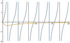
Figure 32: The roots $\mu_{n}$ for $\alpha_{1}=1$, $\bar{\beta}=1/2$, $\alpha_{2}=1$, and $\bar{\beta}_{2}=1$. For $L=2$ this gives $\beta_{1}=1$ and $\beta_{2}=2$.

Equation (182) will provide the mode numbers $\mu_{n}$ for $n=0,1,2,\cdots$, which are used to calculate the wave numbers

$$k_{n}=\frac{\mu_{n}}{L}\ .$$ (183)

Note that $\mu_{0}=0$, and therefore $k_{0}=0$. The solution now takes the form

$$Y_{n}(y) = A_{n}\cos k_{n}y+B_{n}\sin k_{n}y$$ (184)

$$A_{n} = -\frac{\beta_{1}k_{n}}{\alpha_{1}}\,B_{n}\ ,$$ (185)

where $\alpha_{1}\neq 0$. The case of $\alpha_{1}=0$ will be handled separately. Setting $B_{n}=1$ for convenience, the solution (184) can be expressed as

$$Y_{n}(y) = \sin k_{n}y-\frac{\beta_{1}k_{n}}{\alpha_{1}}\cos k_{n}y\ ,$$ (186)

while the general solution takes the form

$$Y(y) = \sum_{n=1}^{\infty}D_{n}Y_{n}(y)\ .$$ (187)

Note that the $n=0$ term does not contribute, and the Fourier coefficients are given by

$$D_{n}=\frac{1}{N_{n}}\int_{0}^{L}dy\,T_{0}(y)Y_{n}(y)\ .$$ (188)

Also note that the modes are orthogonal,

$$\int_{0}^{L}dy\,Y_{n}(y)Y_{m}(y)=0~{}~{}~{}{\rm for}~{}n\neq m\ ,$$ (189)

with the normalization factor $N_{k}$ determined by

$$\int_{0}^{L}dy\,Y_{n}^{2}(y) = \frac{1}{4k_{n}\alpha_{1}^{2}}\Bigg{[}-2\alpha_{1}\beta_{1}k_{n}+2(\beta_{1}^{2}k_{n}^{2}+\alpha_{1}^{2})k_{n}L+$$

$$\hskip 42.67912pt2\alpha_{1}\beta_{1}k_{n}\cos 2k_{n}L+(\beta_{1}^{2}k_{n}^{2}-\alpha_{1}^{2})\sin 2k_{n}L\Bigg{]}\ .$$

That is to say,

$$\int_{0}^{L}dy\,Y_{n}(y)Y_{m}(y)=N_{n}\,\delta_{nm}\ ,$$ (191)

$$N_{n}=\frac{1}{4k_{n}\alpha_{1}^{2}}\Big{[}-2\alpha_{1}\beta_{1}k_{n}+2(\beta_{1}^{2}k_{n}^{2}+\alpha_{1}^{2})k_{n}L+2\alpha_{1}\beta_{1}k_{n}\cos 2k_{n}L+(\beta_{1}^{2}k_{n}^{2}-\alpha_{1}^{2})\sin 2k_{n}L\Big{]}\ .$$

(192)

It is convenient for numerical work to express this in terms of $A_{n}$ and $B_{n}$ coefficients:

$$Y(y) = \sum_{n=1}^{\infty}D_{n}\,\Big{[}-\frac{\beta_{1}k_{n}}{\alpha_{1}}\,\cos k_{n}y+\sin k_{n}y\Big{]}$$ (193)

$$= \sum_{n=1}^{\infty}\Big{[}A_{n}\cos k_{n}y+B_{n}\sin k_{n}y\Big{]}{\rm~{}~{}~{}with}$$ (194)

$$A_{n} = -\frac{\beta_{1}k_{n}}{\alpha_{1}}\,D_{n}~{}~{}~{}{\rm and}~{}~{}~{}B_{n}=D_{n}\ .$$

The temperature $\tilde{T}(y,t)$ is therefore,

$$\tilde{T}(y,t) = \sum_{n=1}^{\infty}\Big{[}A_{n}\cos k_{n}y+B_{n}\sin k_{n}y\Big{]}\,e^{-\kappa\,k_{n}^{2}t}$$ (195)

$$B_{n} = \frac{1}{N_{n}}\int_{0}^{L}dy\,T_{0}(y)Y_{n}(y)$$ (196)

$$A_{n} = -\frac{\beta_{1}k_{n}}{\alpha_{1}}\,B_{n}\ .$$ (197)

For $T_{0}^{a}(y)=T_{1}$ we have

$$B_{n}^{a} = \frac{T_{1}}{N_{n}}\,\left[\frac{1-\cos k_{n}L}{k_{n}}-\frac{\beta_{1}\sin k_{n}L}{\alpha_{1}}\right]\ .$$ (198)

For $T_{0}^{b}(y)=(T_{2}-T_{1})\,y/L$ we have

$$B_{n}^{b} = \frac{T_{2}-T_{1}}{N_{n}\,L}\,\frac{1}{\alpha_{1}k_{n}^{2}}\,\Big{[}\beta_{1}k_{n}-(\alpha_{1}k_{n}L+\beta_{1}k_{n})\cos k_{n}L+(\alpha_{1}-\beta_{1}k_{n}^{2}L)\sin k_{n}L\Big{]}\ ,$$ (199)

with $B_{n}=B_{n}^{a}+B_{n}^{b}$.

Figure 33: The roots $\mu_{n}$ for $\alpha_{1}=0$, $\alpha_{2}=1$, and $\bar{\beta}_{2}=1$. For $L=2$ we have $\beta_{2}=2$.

Let us now consider the case of $\alpha_{1}=0$, so that (182) becomes

$$\tan\mu = \frac{a}{\mu}~{}~{}~{}~{}{\rm with}~{}~{}a=\alpha_{2}/\bar{\beta}_{2}\ .$$ (200)

We can find an approximate solution for large values of $\mu$: since the RHS is very small for $\mu\gg 1$, we must solve $\tan\mu=0$, and therefore $\mu_{n}^{(0)}=n\pi$. The exact solution can be expressed as $\mu_{n}=n\pi+h$, where $0<h\ll 1$, and we find ${\rm LHS}=\tan(n\pi+h)=\tan(h)=h+{\cal O}(h^{2})$. Similarly, ${\rm RHS}=a/(n\pi+h)=(a/n\pi)\big{(}1+h/n\pi\big{)}^{-1}=(a/n\pi)\big{(}1-h/n\pi\big{)}+{\cal O}([h/n]^{2})=a/n\pi-ah+{\cal O}(h^{2}/n^{2})$, thus

$$h=\frac{a}{n\pi}-ah~{}~{}~{}\Rightarrow~{}~{}~{}h=\frac{a}{1+a}\,\frac{1}{n\pi}\ ,$$ (201)

and the first order solution becomes

$$\mu_{n}^{(1)}=n\pi+\frac{a}{1+a}\,\frac{1}{n\pi}+{\cal O}(1/n^{2})\ .$$ (202)

This can be used as an initial guess when using an iteration method to find the $\mu_{n}$. The solution is

$$T(y,t) = \sum_{n=1}^{\infty}A_{n}Y_{n}(y)\,e^{-\kappa\,k_{n}^{2}t}$$ (203)

$$Y_{n}(y) = \cos k_{n}L$$ (204)

$$\int_{0}^{L}dy\,Y_{n}(y)Y_{m}(y) = N_{n}\,\delta_{nm}$$ (205)

$$N_{n} = \frac{1}{4k_{n}}\,\Big{[}2k_{n}L+\sin 2k_{n}L\Big{]}\ ,$$ (206)

and

$$A_{n} = \frac{1}{N_{n}}\int_{0}^{L}dy\,T(y,0)Y_{n}(y)$$ (207)

$$= \frac{T_{1}}{k_{n}}\,\sin k_{n}L+\frac{T_{2}-T_{1}}{k_{n}^{2}L}\,\Big{[}-1+\cos k_{n}L+k_{n}L\sin k_{n}L\Big{]}\ .$$ (208)

C.3 The General Solution

a. BC1: Given Temperatures $T_{1}$ and $T_{2}$

$$T(y,t) = T_{1}+\frac{T_{2}-T_{1}}{L}\,y+\sum_{n=1}^{\infty}B_{n}\,\sin k_{n}y\,e^{-\kappa\,k_{n}^{2}t}$$ (209)

$$B_{n} = \frac{2T_{\scriptscriptstyle\rm A}-2T_{\rm\scriptscriptstyle B}(-1)^{n}}{n\pi}$$ (210)

$$k_{n} = \frac{n\pi}{L}\ .$$ (211)

b. BC2: Given Flux $F$

$$T(y,t) = Fy+\frac{A_{0}}{2}+\sum_{n=1}^{\infty}A_{n}\,\cos k_{n}y\,e^{-\kappa\,k_{n}^{2}t}$$ (212)

$$A_{0} = T_{\scriptscriptstyle\rm A}+T_{\rm\scriptscriptstyle B}$$ (213)

$$A_{n} = 2\,\Big{(}T_{\scriptscriptstyle\rm A}-T_{\rm\scriptscriptstyle B}\Big{)}\,\frac{1-(-1)^{n}}{n^{2}\pi^{2}}$$ (214)

$$k_{n} = \frac{n\pi}{L}\ .$$ (215)

c. BC3: Given $T_{1}$ and $F_{2}$

$$T(y,t) = T_{1}+F_{2}\,y+\sum_{n=0}^{\infty}B_{n}\,\sin k_{n}y\,e^{-\kappa\,k_{n}^{2}t}$$ (216)

$$B_{n} = \frac{4T_{\rm\scriptscriptstyle B}}{(2n+1)\pi}-\frac{8\big{(}T_{\rm\scriptscriptstyle B}-T_{\scriptscriptstyle\rm A}\big{)}}{(2n+1)^{2}\pi^{2}}$$ (217)

$$k_{n} = \frac{(2n+1)\pi}{2L}\ .$$ (218)

d. BC4: Given $T_{2}$ and $F_{1}$

$$T(y,t) = (T_{2}-F_{1}L)+F_{1}\,y+\sum_{n=0}^{\infty}A_{n}\,\cos k_{n}y\,e^{-\kappa\,k_{n}^{2}t}$$ (219)

$$A_{n} = 4T_{\scriptscriptstyle\rm A}\,\frac{(-1)^{n}}{(2n+1)\pi}-8\Big{(}T_{\rm\scriptscriptstyle B}-T_{\scriptscriptstyle\rm A}\Big{)}\,\frac{1-(-1)^{n}}{(2n+1)^{2}\,\pi^{2}}$$ (220)

$$k_{n} = \frac{(2n+1)\pi}{2L}\ .$$ (221)

References

- (1) D.E Burton, Multidimensional discretization of conservation laws for unstructured polyhedral grids, Technical Report UCRL-JC-118306, Lawrence Livermore National Laboratory, August 1994, SAMGOP-94: 2nd International Workshop on Analytical Methods and Process Optimization in Fluid and Gas Mechanics, VNIIEF, Holiday Base, Arzamas-16, Russia, September 10-16, 1994; D.E. Burton, Connectivity structures and differencing techniques for staggered-grid free-Lagrange hydrodynamics, Lawrence Livermore National Laboratory, Report No. UCRL–JC–110555 (1992); D.E. Burton, Consistent finite-volume discretization of hydrodynamic conservation laws for unstructured grids, Lawrence Livermore National Laboratory, Report No. UCRL–JC–118788 (1994).
- (2) M. Shashkov, Algorithms for improved solution robustness, accuracy and mesh adaptivity, LA-UR-15-23913, Los Alamos report (2015).
- (3) A Dawes, C Malone, M Shashkov, Some New Verification Test Problems for Multimaterial Diffusion on Meshes that are Non-Aligned with Material Boundaries, LA-UR-16-24696, Los Alamos report (2016).
- (4) A. Dawes, 3D Multimaterial Polyhedral Methods for Diffusion, MultiMat Conference, Würzberg, Germany, 2015.
- (5) Robert L Singleton Jr, The Planar Sandwich and Other 2D Planar Heat Flow Test Problems in ExactPack, LA-UR-17-20460, Los Alamos report (2017), arXiv:1701.07342v1 [physics.comp-ph].
- (6) ExactPack source code, LA-CC-14-047, available at https://github.com/lanl/exactpack.
- (7) R.V. Garimella and K. Lipnikov, Solution of the diffusion equation in multimaterial domains by subdivision of elements along reconstructed interface Int. J. Numer. Meth. Fluids (2011) 1423.
- (8) E. Kikinzon, Y. Kuznetsov, and M. Shashkov, New algorithm for solving multimaterial diffusion problems on mesh non-aligned with material interfaces, LA-UR-16-21548, Los Alamos Report (2016).
- (9) E. Kikinzon, Y. Kuznetsov, and M. Shashkov, Approximate static condensation algorithm for solving multimaterial diffusion problems on meshes non-aligned with material interfaces, J. Comp. Phys, 347, 416 (2017).
- (10) Personal notes, R. Singleton, Summer 2017.
- (11) Paul W Berg and James L McGregor, Elementary Partial Differential Equations, Holden Day (1966).
- (12) Walter Rudin, Principles of Mathematical Analysis, McGraw-Hill, third edition (1976).
- (13) James R. Kamm, Jerry S. Brock, Christopher L. Rousculp, William J. Rider, Verification of an ASCI Shavano Project Hydrodynamics Algorithm, LA-UR-03-6999 Los Alamos Report (2003).