The Gauss quadrature for general linear functionals, Lanczos algorithm, and minimal partial realization

Abstract

The concept of Gauss quadrature can be generalized to approximate linear functionals with complex moments. Following the existing literature, this survey will revisit such generalization. It is well known that the (classical) Gauss quadrature for positive definite linear functionals is connected with orthogonal polynomials, and with the (Hermitian) Lanczos algorithm. Analogously, the Gauss quadrature for linear functionals is connected with formal orthogonal polynomials, and with the non-Hermitian Lanczos algorithm with look-ahead strategy; moreover, it is related to the minimal partial realization problem. We will review these connections pointing out the relationships between several results established independently in related contexts. Original proofs of the Mismatch Theorem and of the Matching Moment Property are given by using the properties of formal orthogonal polynomials and the Gauss quadrature for linear functionals.

1 Introduction

Let $A$ be an $N\times N$ Hermitian positive definite matrix and $\mathbf{v}$ a vector so that $\mathbf{v}^{*}\mathbf{v}=1$, where $\mathbf{v}^{*}$ is the conjugate transpose of $\mathbf{v}$. Consider the specific linear functional $\mathcal{L}$ on the space of polynomials defined by

$$\mathcal{L}(\lambda^{j}):=\mathbf{v}^{*}A^{j}\mathbf{v}=m_{j},\quad j=0,1,\dots,$$ (1.1)

where $m_{0},m_{1},\dots$ are real numbers known as the moments of $\mathcal{L}$. The functional $\mathcal{L}$ can be expressed as the Riemann-Stieltjes integral with a non-decreasing positive distribution function $\mu(\lambda)$ supported on the real axis having finitely many points of increase; see, e.g, (LieStrBook13, , Section 3.5),(GolMeuBook10, , Section 7.1), and (ChiBook78, , Chapter II, Section 3). For $1\leq n\leq N$, the $n$-node (classical) Gauss quadrature approximating $\mathcal{L}$ is given by the unique $n$-node quadrature formula which matches the first $2n$ moments, i.e.,

$$\mathcal{L}(\lambda^{j})=\int_{\mathbb{R}}\lambda^{j}\,\textrm{d}\mu(\lambda)=\sum_{i=1}^{n}\omega_{i}\,(\lambda_{i})^{j},\quad j=0,\dots,2n-1,$$

with $\omega_{i}$ positive weights and $\lambda_{i}$ positive distinct nodes. Classical results of the Gauss quadrature can be found, e.g., in (SzeBook39, , Chapters III and XV), (ChiBook78, , Chapter I, Section 6), Gau81 , (GauBook04, , Section 1.4), (gautschi2011numerical, , Chapter 3.2), (LieStrBook13, , Section 3.2). The linear functional $\mathcal{L}$ can be associated with a Jacobi matrix $J_{n}$ which is an $n\times n$ real symmetric tridiagonal matrix. For every function $f$ defined on the spectrum of $A$ and $J_{n}$, the matrix $J_{n}$ gives an algebraic expression for the Gauss quadrature, i.e.,

$$\mathbf{v}^{*}f(A)\,\mathbf{v}=\int_{\mathbb{R}}f(\lambda)\,\textrm{d}\mu(\lambda)\approx\sum_{i=1}^{n}\omega_{i}\,f(\lambda_{i})=\mathbf{e}_{1}^{T}f(J_{n})\,\mathbf{e}_{1},$$ (1.2)

where $f(A)$ and $f(J_{n})$ are matrix functions, and $\mathbf{e}_{1}$ is the first vector of the Euclidean basis (with $\mathbf{e}_{1}^{T}$ the transpose). The matrix $J_{n}$ can be obtained by $n$ iterations of the Hermitian Lanczos algorithm with inputs $A$ and $\mathbf{v}$. Indeed, $J_{n}=V_{n}^{*}AV_{n}$, where $V_{n}$ is the matrix given by the Lanczos algorithm whose columns are an orthonormal basis of the Krylov subspace $\{\mathbf{v},A\mathbf{v},\dots,A^{n-1}\mathbf{v}\}$. Hence the Hermitian Lanczos algorithm with input $A,\mathbf{v}$ gives a matrix formulation of the Gauss quadrature for $\mathcal{L}$. Figure 1 (see (LieStrBook13, , Figure 3.2)) represents the connections described above. Such connections can be derived by the properties of orthogonal polynomials; a detailed explanation can be found, e.g., in (LieStrBook13, , Chapter 3) and GolMeuBook10 (note that the relationships between the Conjugate Gradient method, Lanczos algorithm, and orthogonal polynomials were already pointed out by Hestenes and Stiefel in their seminal paper published in 1952 (HesSti52, , Sections 14–17)).

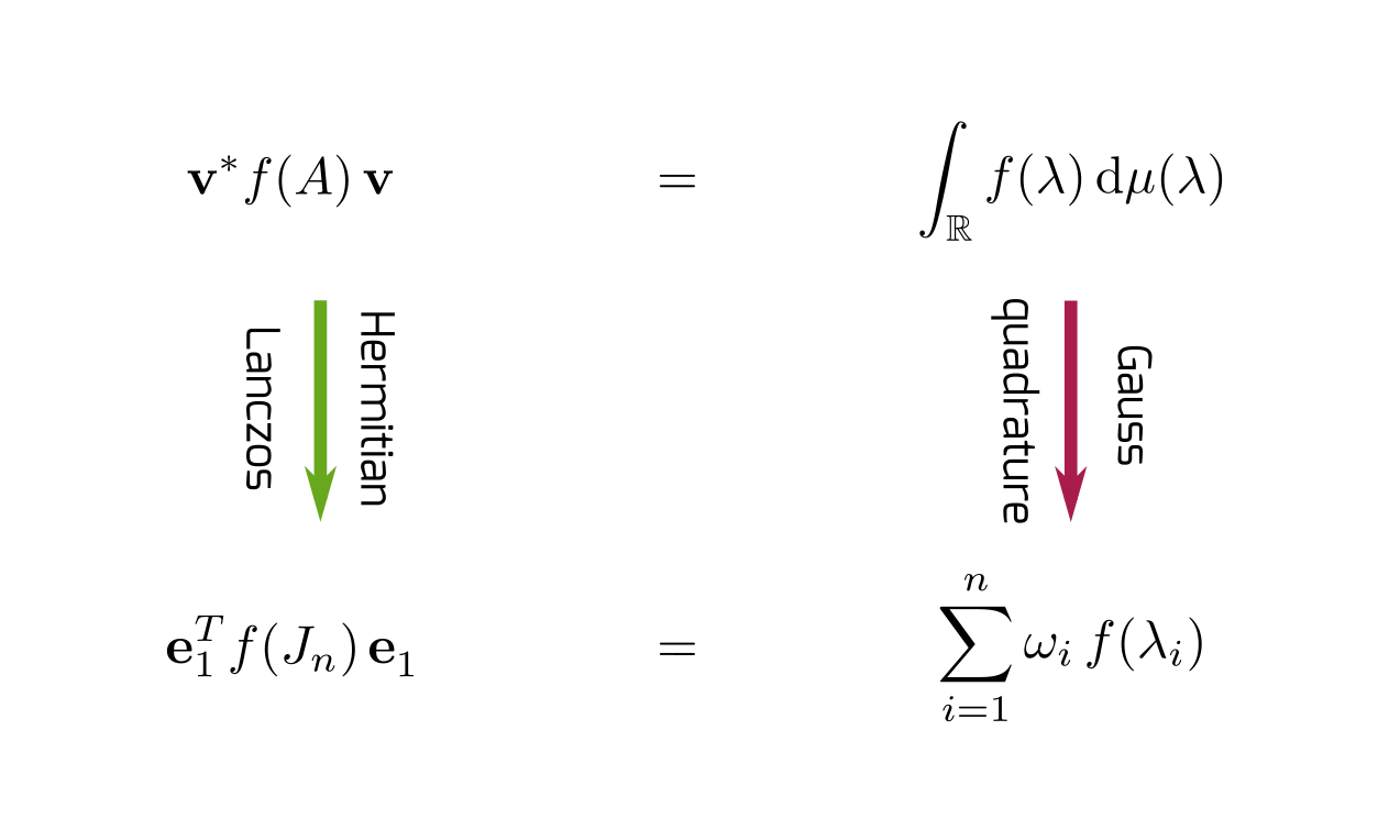
Figure 1: Visualization of the connections between the (classical) Gauss quadrature and the Hermitian Lanczos algorithm.

This survey deals with the extension of the connections summarized in Figure 1 to the case of a general linear functional defined on the space $\mathcal{P}$ of the polynomials with generally complex coefficients, $\mathcal{L}:\mathcal{P}\rightarrow\mathbb{C}$. We point out that, if not specified otherwise, we will consider linear functionals without the underlying assumption that they are determined by a matrix bilinear form analogous to (1.1). The survey will revisit the Gauss quadrature for linear functionals, its matrix formulation, its connection with the non-Hermitian Lanczos algorithm with look-ahead strategy, and its relationship with the minimal partial realization problem. Furthermore, the connections between the incurable breakdown, the exactness of the Gauss quadrature, and the minimal realization problem, will be examined with giving an original proof of the Mismatch Theorem (first proved in (Tay82, , Theorem 4.2)). The proof easily follows from the properties we will present, providing a different interpretation of the Theorem in terms of formal orthogonal polynomials roots and nodes of the Gauss quadrature for linear functionals.

Information about the topics mentioned above and their mutual relationships are scattered in the literature. The survey aims to describe such topics and their connections from the point of view of formal orthogonal polynomials. We hope that such a presentation will be of interest for readers working in related different areas.

Regarding the formal orthogonal polynomials and the Gauss quadrature generalization, we will mainly follow the book DraBook83 by Draux where the Gauss quadrature is extended for the approximation of real-valued linear functionals. More precisely, a straightforward extension of Draux’s definition to the case of complex-valued linear functionals will be presented. The more recent Gauss quadrature definitions in Mil03 and in PozPraStr16 ; PozPraStr18 , obtained independently of DraBook83 , can be seen as a generalization to the complex quasi-definite case. Indeed, for a real quasi-definite linear functional the quadratures in DraBook83 ; Mil03 ; PozPraStr16 ; PozPraStr18 are equivalent. However, some results in PozPraStr16 ; PozPraStr18 do not have a counterpart in the real setting of DraBook83 (for instance, formal orthonormal polynomials may have complex coefficients). The case of a quasi-definite linear functional is simpler to treat; see, e.g., ChiBook78 ; PozPraStr16 ; PozPraStr18 . The survey will first recall the primary results associated with quasi-definite functionals and then deal with the case of a general linear functional.

This survey approaches the Lanczos algorithm in a finite dimensional setting. Hence we will not treat infinite dimensional problems. For infinite dimensional problems related to positive definite linear functionals refer, e.g., to (ChiBook78, , Chapter II, Section 3, in particular Theorem 3.1). For the relationship with infinite dimensional Krylov subspace methods refer, e.g., to VorBook65 , GunHerSac14 , and (malek2015, , Chapter 5) where many references to original works can be found.

Throughout the survey, we will consider only computations in exact arithmetic. Since rounding errors substantially affect computations with short recurrences, the results described in this survey cannot be applied to finite precision computations without a thorough analysis. Such analysis is out of the scope of this survey. The interested reader can refer to Bai94 and Day93 ; Day97 for analysis of the non-Hermitian Lanczos algorithm in finite precision (assuming no breakdown); see also the related works BaiDayYe99 ; TonYe00 ; PaiPanZem14 . As pointed out in (LieStrBook13, , Sections 2.5.6 and 5.11), in finite precision arithmetic the short recurrences cannot preserve the biorthogonality or even the linear independence of the computed Krylov subspace basis. Therefore look-ahead techniques for the non-Hermitian Lanczos have a limited impact in computing sufficiently well-conditioned basis when dealing with the loss of biorthogonality. The interplay of look-ahead techniques and rounding errors in practical computations is still an open issue.

The paper is organized as follows. Section 2 summarizes basic results of quasi-definite linear functionals. Section 3 recalls properties of formal orthogonal polynomials and of quasi-orthogonal polynomials with respect to a linear functional $\mathcal{L}:\mathcal{P}\rightarrow\mathbb{C}$. The concept of Gauss quadrature for linear functionals and its matrix interpretation can be found respectively in Section 4 and Section 5. The Gauss quadrature connections with the minimal partial realization problem and with the look-ahead Lanczos algorithm are described respectively in Section 6 and Section 7. Section 8 concludes the survey summarizing the links between the Gauss quadrature, minimal partial realization, and look-ahead Lanczos algorithm.

2 Quasi-definite linear functionals

We start recalling several results for quasi-definite linear functionals following the description in our previous works with Zdeněk Strakoš PozPraStr16 ; PozPraStr18 . These results will be extended to the more challenging general case in the remaining sections.

Let $\mathcal{L}:\mathcal{P}\rightarrow\mathbb{C}$ be a linear functional with complex moments,

$$\mathcal{L}(\lambda^{k})=m_{k},\quad k=0,1,\ldots\,.$$ (2.1)

An $n$-degree polynomial $p_{n}(\lambda)\in\mathcal{P}$ is called formal orthogonal polynomial (FOP) when it satisfies the orthogonality conditions with respect to $\mathcal{L}$

$$\mathcal{L}(p_{n}\,\lambda^{j})=0,\quad\textrm{ for }j=0,\dots,n-1;$$

refer, e.g., to (DraBook83, , Introduction and Section 1.1) and (Bre02, , Chapter 2). Notice that in BreBook80 $p_{n}(\lambda)$ is referred as general orthogonal polynomial; cf. the concept of weak orthogonal polynomial in (Krall1966, , definition on p. 137) and (KwoLit97, , Section 2). The subindex $n$ in the polynomial notation $p_{n}(\lambda)$ will always stand for the degree of the polynomial and we will not emphasize it further on. Moreover, whenever appropriate the argument $\lambda$ will be skipped for simplicity of notation.

Denoting with $\mathcal{P}_{k}\subset\mathcal{P}$ the subspace of polynomials of degree at most $k$, the following classes of linear functionals can be defined (see, e.g., Theorem 3.1, Definition 3.2, Theorem 3.4 and the subsequent Corollary in (ChiBook78, , Chapter I), Theorem 1 and the subsequent Remark in (LorWaaBook92, , Chapter VII)).

Definition 2.1

The linear functional $\mathcal{L}$ is said to be quasi-definite on $\mathcal{P}_{k}$ if there exist unique FOPs $p_{0}(\lambda),\dots,p_{k}(\lambda)$ (we always use the term “unique” for a polynomial in the sense of unique up to multiplication by a nonzero scalar) satisfying the conditions

$$\mathcal{L}(p_{j}p_{n})=0,\textrm{ for }j\neq n,\textrm{ and }\,\mathcal{L}(p_{n}^{2})\neq 0.$$

A linear functional is said to be positive definite on $\mathcal{P}_{k}$ if in addition $p_{0}(\lambda),\dots,p_{k}(\lambda)$ are real polynomials, and $\mathcal{L}(p_{n}^{2})>0$, for $n=0,\dots,k$.

Note that the definition above is equivalent to the ones in (PozPraStr16, , Definition 2.1 and Definition 3.1) and (PozPraStr18, , Definition 1.1).

If a FOP $p_{n}$ is such that $\mathcal{L}(p_{n}^{2})=1$, then it is a formal orthonormal polynomial. A beautiful summary about FOPs in the quasi-definite case can be found in the book by Chihara ChiBook78 (notice that Chihara used the simplified term orthogonal polynomials instead of formal orthogonal polynomials). A sequence of formal orthonormal polynomials $p_{0}(\lambda),\dots,p_{k}(\lambda)$ satisfy the three-term recurrence

$$\beta_{n}p_{n}(\lambda)=(\lambda-\alpha_{n-1})p_{n-1}(\lambda)-\beta_{n-1}p_{n-2}(\lambda),\quad\quad n=1,\dots,k,$$ (2.2)

where $\beta_{0}=0$, $p_{-1}(\lambda)=0$, $p_{0}(\lambda)={1}/{\sqrt{m_{0}}}$ and the coefficients $\alpha_{n-1}$, $\beta_{n}$ are given by

$$\alpha_{n-1}=\mathcal{L}(\lambda p_{n-1}p_{n-1}),\,\,\,\beta_{n}=\mathcal{L}(\lambda p_{n-1}p_{n}).$$

see, e.g., (ChiBook78, , Chapter I, Section 4), (BreBook80, , Theorem 2.4). Notice that in order to avoid ambiguity, we always take the principal value of the complex square root, i.e., we consider $arg(\sqrt{c})\in(-\pi/2,\pi/2]$. The recurrences (2.2) can be written in the compact form as

$$\lambda\,\mathbf{p}(\lambda)=J_{n}\mathbf{p}(\lambda)+\beta_{n}p_{n}(\lambda)\mathbf{e}_{n},\quad n=1,\dots,k,$$

where $\mathbf{p}(\lambda)=[p_{0}(\lambda),p_{1}(\lambda),\dots,p_{n-1}(\lambda)]^{T}$, $\mathbf{e}_{n}$ is the $n$th vector of the Euclidean basis, and $J_{n}$ is the $n$th complex Jacobi matrix

$$J_{n}=\left[\begin{matrix}\alpha_{0}&\beta_{1}&&\\ \beta_{1}&\alpha_{1}&\ddots&\\ \vspace{4pt}&\ddots&\ddots&\beta_{n-1}\\ &&\beta_{n-1}&\alpha_{n-1}\end{matrix}\right],\quad n=1,\dots,k;$$ (2.3)

more information about complex Jacobi matrices and their properties can be found, e.g., in Bec01 and in (PozPraStr16, , in particular Section 4).

Given a smooth enough function $f(\lambda)$, the Gauss quadrature for quasi-definite linear functionals considered in PozPraStr16 ; PozPraStr18 has the form

$$\mathcal{G}_{n}(f):=\sum_{i=1}^{\ell}\sum_{j=0}^{s_{i}-1}\omega_{i,j}\,f^{(j)}(\lambda_{i}),\quad n=s_{1}+\,\cdots\,+s_{\ell},$$

and satisfies the following properties.

• G1: the quadrature $\mathcal{G}_{n}(f)$ has maximal degree of exactness $2n-1$, i.e., it is exact for all polynomials of degree at most $2n-1$;

• G2: the quadrature $\mathcal{G}_{n}(f)$ is well-defined and it is unique. Moreover, Gauss quadratures with a smaller number of weights also exist and they are unique;

• G3: the quadrature $\mathcal{G}_{n}(f)$ can be written as the matrix form $m_{0}\,\mathbf{e}_{1}^{T}f(J_{n})\mathbf{e}_{1}$, where $J_{n}$ is the complex Jacobi matrix associated with $\mathcal{L}$.

A quadrature having properties G1, G2 and G3 exists if and only if the linear functional $\mathcal{L}$ is quasi-definite on $\mathcal{P}_{n}$; see (PozPraStr16, , Section 7, in particular Corollaries 7.4 and 7.5) and (PozPraStr18, , Theorem 3.1).

Property G3 corresponds to the so called Matching Moment Property of the complex Jacobi matrix, i.e., if the complex numbers $m_{0},\dots,m_{2n-1}$ define a quasi-definite linear functional (2.1) with associated Jacobi matrix $J_{n}$ (here and in the following the simplified term quasi-definite linear functional and positive definite linear functional will stand for linear functionals that are quasi-definite and positive definite on the space of polynomials of sufficiently large degree), then

$$m_{0}\,\mathbf{e}_{1}^{T}\,(J_{n})^{j}\mathbf{e}_{1}=m_{j},\quad j=0,\dots,2n-1;$$ (2.4)

see (PozPraStr16, , Section 5). In (FreHoc93, , Theorem 2) the Matching Moment Property was proved for a quasi-definite linear functional given by

$$\mathcal{L}(f)=\mathbf{w}^{*}f(A)\mathbf{v},$$

where $A$ is a complex matrix and $\mathbf{w},\mathbf{v}$ are vectors (compare also with (Cyb87, , Theorem 1)). In Str09 it was derived by the Vorobyev method of moments (see in particular Chapter III of VorBook65 ).

3 Polynomials and orthogonality

Let $\mathcal{L}:\mathcal{P}\rightarrow\mathbb{C}$ be a linear functional with moments $m_{0},m_{1},\dots$. Consider the sequence of $k$-dimensional Hankel matrices

$$H_{k-1}=H(1:k;1:k)=\left[\,\,\begin{matrix}\vspace{3pt}m_{0}&m_{1}&\ldots&m_{k-1}\\ m_{1}&m_{2}&\ldots&m_{k}\\ \vdots&\vdots&&\vdots\\ m_{k-1}&m_{k}&\ldots&m_{2k-2}\end{matrix}\,\,\right],\quad k=1,2,\ldots\,,$$ (3.1)

with the corresponding determinant $\Delta_{k-1}$ (the notation $A(i:j;\ell:n)$ stands for the submatrix of $A$ composed of the elements in the rows from $i$ to $j$ and in the columns from $\ell$ to $n$). Setting ${\bf m}_{k-1}$ as the vector

$${\bf m}_{k-1}=H(1:k;k+1)=[m_{k},\ldots,m_{2k-1}]^{T},$$

we are interested in the properties of the linear system

$$H_{k-1}\,{\bf c}=-{\bf m}_{k-1}.$$ (3.2)

The solution of Hankel systems, and many related properties of Hankel matrices, have been extensively treated in the literature; see, e.g, to the seminal paper by Stieltjes (Sti1894, , Sections 8–11, pp. 624–630) (please notice that we refer to the English translation published by Springer in 1993), the monographs (ChiBook78, , Chapter I), (DraBook83, , Chapter 1), Ioh82 , (HeiRos84, , Part I), and (BulVBaBook97, , Chapter 2), and the paper (GraLin83, , Section 2). Here, we refer in particular to some results in Section 1.2 of DraBook83 ; their straightforward generalization to the complex case is equivalent to Theorems 3.1 and 3.2 given in this section; see also Theorem 7 in (GanBook59, , Chapter XV, §10) in the context of infinite Hankel matrices with finite rank. We do not report the proofs of Theorems 3.1 and 3.2 since they are based on the study of Hankel matrices, and they would lead us too far from the main point of the survey. We will use them as the starting point of our presentation.

Theorem 3.1

Assume that $\Delta_{k-1}\neq 0$, then $\Delta_{k}=0$ if and only if

$$-m_{2k}=c_{0}m_{k}+c_{1}m_{k+1}+\ldots+c_{k-1}m_{2k-1},$$ (3.3)

where ${\bf c}=[c_{0},\ldots,c_{k-1}]^{T}$ is the unique solution of the linear system (3.2). Moreover, if $\Delta_{k-1}\neq 0$ and $\Delta_{k}=\Delta_{k+1}=\ldots=\Delta_{k+j-1}=0$ for $j\geq 1$, then $\Delta_{k+j}=0$ if and only if

$$-m_{2k+j}=c_{0}m_{k+j}+c_{1}m_{k+j+1}+\ldots+c_{k-1}m_{2k+j-1}.$$ (3.4)

As a consequence, we get the following theorem; see (DraBook83, , Property 1.6).

Theorem 3.2

Assume that $\Delta_{k-1}\neq 0$ and $\Delta_{k}=\Delta_{k+1}=\ldots=\Delta_{k+j-1}=0$. Then the system

$$H_{k+j-1}\,{\bf b}=-{\bf m}_{k+j-1}$$ (3.5)

has (infinitely many) solutions if and only if $\Delta_{k+j}=\Delta_{k+j+1}=\ldots\Delta_{k+2j-1}=0$.

The following theorem gives necessary and sufficient conditions for the existence (and uniqueness) of a FOP $p_{n}(\lambda)$ of degree $n$; see (DraBook83, , Property 1.14).

Theorem 3.3

Let $\mathcal{L}:\mathcal{P}\rightarrow\mathbb{C}$ be a linear functional. An $n$-degree monic FOP exists if and only if one of the following conditions is satisfied.

• $\Delta_{n-1}\neq 0$ (unique monic FOP);

• $\Delta_{k-1}\neq 0$ and $\Delta_{k}=\Delta_{k+1}=\ldots=\Delta_{n-1}=\ldots=\Delta_{2n-k-1}=0$ (infinitely many monic FOPs);

where $\Delta_{0},\Delta_{1},\dots$ are the determinants of the Hankel submatrices $H_{0},H_{1},\dots$ composed of the moments of $\mathcal{L}$.

Proof

A monic FOP of degree $n$

$$\pi_{n}(\lambda)=\lambda^{n}+c_{n-1}\lambda^{n-1}+\ldots+c_{1}\lambda+c_{0}$$

exists if and only if $\mathcal{L}(\lambda^{j}\pi_{n})=0$, for $j=0,\ldots,n-1$, which gives the linear system (3.2) with $k=n$. Therefore if $\Delta_{n-1}\neq 0$, then the polynomial $\pi_{n}(\lambda)$ exists and is unique. If $\Delta_{n-1}=0$, then necessary and sufficient conditions for the existence of $\pi_{n}(\lambda)$ are given by Theorem 3.2: for $\Delta_{k-1}\neq 0$ and $\Delta_{k}=\Delta_{k+1}=\ldots=\Delta_{n-1}=0$, there exist infinitely many $\pi_{n}(\lambda)$ if and only if $\Delta_{n}=\Delta_{n+1}=\ldots\Delta_{2n-k-1}=0$. ∎

Note that by Theorem 3.3, a linear functional $\mathcal{L}$ is quasi-definite on $\mathcal{P}_{k}$ if and only if $\Delta_{j}\neq 0$, for $j=0,1,\dots,k$; see, e.g., (ChiBook78, , Chapter I, Theorem 3.1).

The second item of Theorem 3.3 can be interpreted in the following way: consider the sequence $\Delta_{0},\Delta_{1},\Delta_{2},\dots$. Let $R=R(n-1)$ be the number of zeros in the sequence between $\Delta_{n-1}$ and the first nonzero element in the sequence after $\Delta_{n-1}$, i.e., $\Delta_{n-1+j}=0$ for $j=1,\ldots,R$ and $\Delta_{n+R}\neq 0$. Note that the parameters $R(n-1)$ are known as Kronecker index, and the differences $R(n)-R(n-1)$ as Euclidean indices; see BulVBaBook97 ; Kai80 . Let $L=L(n-1)$ be the number of zeros in the sequence between $\Delta_{n-1}$ and the last nonzero element in the sequence before $\Delta_{n-1}$, i.e., $\Delta_{n-1-j}=0$ for $j=1,\ldots,L$ and $\Delta_{n-L-2}\neq 0$. A FOP of degree $n$ exists if and only if $R(n-1)>L(n-1)$. Roughly said, there are “more consecutive zeros to the right than to the left”.

Among the formal orthogonal polynomials the following cases can be distinguished; see Definition on p. 47 of DraBook83 .

Definition 3.4

A formal orthogonal polynomial (FOP) $p_{n}(\lambda)$ is called regular when $\Delta_{n-1}\neq 0$ (i.e., when it is unique), while it is called singular when $\Delta_{n-1}=0$ (i.e., when it is not unique).

Proposition 3.5

Let $p_{k}$ be a regular FOP and $j\geq 0$. Then $\mathcal{L}(p_{k}q)=0$ for every $q\in\mathcal{P}_{k+j}$ if and only if $\Delta_{k}=\Delta_{k+1}=\ldots=\Delta_{k+j}=0$.

Proof

Without loss of generality, let us assume $p_{k}$ to be monic. The conditions $\mathcal{L}(p_{k}\,\lambda^{k+i})=0$, for $i=0,\dots,j$, lead to the system

$$-m_{2k+i}=c_{0}m_{k+i}+c_{1}m_{k+i+1}+\ldots+c_{k-1}m_{2k+i-1},\quad i=0,\dots,j,$$

with $c_{0},\dots,c_{k-1}$ the unique solution of the linear system (3.2). Theorem 3.1 concludes the proof.

Knowing all the integers $k$ such that $\Delta_{k}=0$ allows determining all the integers $n$ for which a FOP $p_{n}(\lambda)$ exists.

Example 1. If the zero-nonzero pattern of the sequence of Hankel determinants $\Delta_{k}$ is

$$\begin{array}[]{cccccccccccccccc}\Delta_{k}&=&\ast&\ast&0&\ast&\ast&0&0&0&0&\ast&0&0&0&\ast\\ k&=&0&1&2&3&4&5&6&7&8&9&10&11&12&13\end{array},$$

then the FOPs of degree $3,8,9,12$ and $13$ do not exist. There exist regular FOPs of degree $1,2,4,5,10$ and $14$ and singular FOPs of degree $6,7$ and $11$.

In order to fill the gaps in FOP sequences, we consider polynomials satisfying the following property.

Definition 3.6

The polynomial $p_{n}(\lambda)$ is called quasi-orthogonal of order $k$ (or $k$-quasi-orthogonal), with $k<n$, when

$$\mathcal{L}(p_{n}\lambda^{j})=0,\quad j=0,\ldots,n-k-1.$$

Quasi-orthogonal polynomials of order $1$ were introduced by Riesz in Rie23 and then generalized to any order by Chihara in Chi57 ; see also (DraBook83, , Definition 1.1, p. 51), Dra90 , Dra16 , and compare the definition with the concept of inner formal orthogonal polynomials given in (hochbruck:1996, , Definition 5.2) and of left and right quasi-formally biorthogonal polynomials in (Fre93b, , Definition 3.3). Note that Definition 3.6 does not require $k$ to be minimal, i.e., it is not necessary that $\mathcal{L}(p_{n}\lambda^{n-k})\neq 0$. Thus a $k$-quasi-orthogonal polynomial of degree $n$ is also $j$-quasi-orthogonal for $j=k+1,\dots,n-1$. Also, any formal orthogonal polynomial of degree $n$ is $k$-quasi-orthogonal for $k=1,\dots,n-1$.

If $\Delta_{k-1}\neq 0$, then an $(n-k)$-quasi orthogonal polynomial of degree $n$ exists for every $n$ larger than $k$; see, e.g., (Fre93b, , Lemma 3.4). The following theorem will prove it together with the characterization of such polynomials; see discussion on pp. 47–51 of DraBook83 .

Theorem 3.7

Let $\Delta_{0},\Delta_{1},\dots$ be the Hankel determinants associated with the linear functional $\mathcal{L}$. Let $\Delta_{k-1}\neq 0$, and $\Delta_{k-1+i}=0$ for $i=1,\ldots,j$, and let $\pi_{k}(\lambda)$ be the regular monic FOP with respect to $\mathcal{L}$. Then all the monic $i$-quasi-orthogonal polynomials $\pi_{k+i}(\lambda)$ for $i=1,\dots,j$ are of the form

$$\pi_{k+i}(\lambda)=\pi_{k}(\lambda)\prod_{t=1}^{i}(\lambda-\eta_{t}),\quad\eta_{t}\in\mathbb{C}.$$ (3.6)

Proof

The proof is by induction on $i$. Let $i=1$. By Proposition 3.5, $\Delta_{k}=0$ if and only if $\pi_{k}(\lambda)$ is orthogonal to all polynomials of degree $k$. Therefore $\lambda\pi_{k}(\lambda)$ is a monic polynomial of degree $k+1$ that is orthogonal to $\mathcal{P}_{k-1}$:

$$\mathcal{L}(\lambda\,\pi_{k}\,q)=\mathcal{L}(\pi_{k}\,(\lambda\,q))=0,\quad\textrm{ for }q(\lambda)\in\mathcal{P}_{k-1}.$$

Moreover, any polynomial of the form $(\lambda-\alpha)\pi_{k}(\lambda)$, $\alpha\in\mathbb{C}$, is a monic $1$-quasi-orthogonal polynomial. On the other side, assume that $p_{k+1}(\lambda)$ is an arbitrary monic polynomial of degree $k+1$ that is orthogonal to $\mathcal{P}_{k-1}$. Then the polynomial $\lambda\pi_{k}(\lambda)-p_{k+1}(\lambda)$ has the following two properties:

• it is of degree $k$,

• it is orthogonal to $\mathcal{P}_{k-1}$.

Hence the uniqueness of $\pi_{k}(\lambda)$ gives $\lambda\pi_{k}(\lambda)-p_{k+1}(\lambda)=\beta\pi_{k}(\lambda)$ for a certain complex number $\beta$, i.e.,

$$p_{k+1}(\lambda)=(\lambda-\beta)\,\pi_{k}(\lambda),\quad\textrm{ for some }\beta\in\mathbb{C}.$$

Set $i$ between $2$ and $j-1$, and assume that all the monic $i$-quasi-orthogonal polynomials of degree $k+i$ are of the form (3.6). By Proposition 3.5, $\Delta_{k}=\Delta_{k+1}=\ldots=\Delta_{k+i}=0$ if and only if $\pi_{k}(\lambda)$ is orthogonal to all polynomials of degree $k+i$. Therefore $\lambda\pi_{k+i}(\lambda)$ is a monic polynomial of degree $k+i+1$ that is orthogonal to $\mathcal{P}_{k-1}$:

$$\mathcal{L}(\lambda\,\pi_{k+i}\,q)=\mathcal{L}(\pi_{k}\,(\lambda\,(\lambda-\eta_{1})\cdots(\lambda-\eta_{i})\,q))=0,\quad\textrm{ for }q(\lambda)\in\mathcal{P}_{k-1}.$$

Clearly, $(\lambda-\alpha)\pi_{k+i}(\lambda)$ is a monic $(i+1)$-quasi-orthogonal polynomial of degree $k+i+1$, for any complex number $\alpha$. It remains to prove that an arbitrary monic polynomial of degree $k+i+1$ that is orthogonal to $\mathcal{P}_{k-1}$ is of the form $(\lambda-\beta)\pi_{k+i}(\lambda)$, where $\beta$ is a certain complex number, and $\pi_{k+i}(\lambda)$ is a polynomial of the form (3.6). It can be done similarly to the case $i=1$. ∎

Proposition 3.8

Let $\Delta_{0},\Delta_{1},\dots$ be the Hankel determinants associated with the linear functional $\mathcal{L}$ such that $\Delta_{k-1}\neq 0$ and $\Delta_{k+i}=0$ for $i=0,\dots,2j-1$. Then for $i=0,\dots,j$, $p_{k+i}(\lambda)$ is a FOP if and only if it is $i$-quasi-orthogonal.

Proof

Clearly any FOP of degree $k+i$ is $i$-quasi-orthogonal. Vice versa if $p_{k+i}(\lambda)$ is $i$-quasi-orthogonal, then it satisfies (3.6). By Proposition 3.5, $p_{k}(\lambda)$ is orthogonal to $\mathcal{P}_{k+2j-1}$. Therefore if $q(\lambda)\in\mathcal{P}_{k+i-1}$, then $\mathcal{L}(p_{k+i}q)=\mathcal{L}(p_{k}(\lambda-\eta_{1})\cdots(\lambda-\eta_{i})q)=0$ for $i=0,\dots,j$. ∎

Consider the sequence of polynomials

$$p_{0}(\lambda),p_{1}(\lambda),p_{2}(\lambda),\dots$$ (3.7)

constructed in the following way: $p_{n}(\lambda)$ is a regular FOP (when possible) or $p_{n}(\lambda)$ is a $(n-k)$-quasi-orthogonal polynomial, where $p_{k}(\lambda)$ is the last regular FOP before $p_{n}(\lambda)$. For later convenience, we consider every nonzero choice for $p_{0}(\lambda)$ as a regular FOP. Let us denote by $\nu{(0)},\nu{(1)},\nu{(2)},\dots$ all the indexes for which $p_{\nu{(j)}}(\lambda)$ is a regular FOP, i.e., $\Delta_{\nu{(j)-1}}\neq 0$ (setting $p_{\nu(0)}(\lambda)=p_{0}(\lambda)\neq 0$, and $\nu(j+1)=\infty$ when $p_{\nu(j)}(\lambda)$ is the last of the regular FOPs). By Theorem 3.7, the quasi-orthogonal polynomials between two consecutive regular FOPs $p_{\nu(j)}(\lambda),p_{\nu(j+1)}(\lambda)$ satisfy the recurrences

$$\beta_{n}p_{n}(\lambda)=\lambda p_{n-1}(\lambda)-\sum_{i=\nu(j)}^{n-1}\alpha_{n,i}p_{i}(\lambda),\quad n=\nu(j)+1,\dots,\nu(j+1)-1,$$ (3.8)

for some coefficients $\alpha_{n,i}\in\mathbb{C}$ and $\beta_{n}\neq 0$; see (DraBook83, , Theorem 1.5 and Remark 1.2). Notice that any choice of $\alpha_{n,i}$ and $\beta_{n}\neq 0$ defines a $(n-\nu(j))$-quasi-orthogonal polynomial. In particular, there exist families of such polynomials satisfying the two-term recurrences

$$\beta_{n}p_{n}(\lambda)=(\lambda-\alpha_{n,n-1})p_{n-1}(\lambda),\quad n=\nu(j)+1,\dots,\nu(j+1)-1;$$ (3.9)

fixing $\alpha_{n,n-1}=0$ gives even simpler recurrences.

Setting $n=\nu{(j+1)}$ for some $j\geq 0$, the regular FOP $p_{n}(\lambda)$ satisfies (see (DraBook83, , Theorem 1.5 and Remark 1.2) and (GraLin83, , Theorem 2))

$$\beta_{n}p_{n}(\lambda)=\lambda p_{n-1}(\lambda)-\sum_{i=\nu(j)}^{n-1}\alpha_{n,i}p_{i}(\lambda)-\gamma_{n}p_{\nu(j-1)}(\lambda),$$ (3.10)

with $p_{\nu(-1)}(\lambda)=p_{-1}(\lambda)=0$, $\beta_{n}$ a nonzero coefficient, $\gamma_{\nu(1)}=0$,

$$\gamma_{n}=\frac{\mathcal{L}(\lambda p_{n-1}p_{\nu(j)-1})}{\mathcal{L}(p_{\nu(j)-1}p_{\nu(j-1)})}\neq 0,\quad j\geq 1,$$

and $\alpha_{n,i}$ given by

$$\left[\begin{array}[]{ccc}\mathcal{L}(p_{\nu(j)}p_{\nu(j)})&\ldots&\mathcal{L}(p_{\nu(j)}p_{n-1})\\ \vdots&&\vdots\\ \mathcal{L}(p_{n-1}p_{\nu(j)})&\ldots&\mathcal{L}(p_{n-1}p_{n-1})\end{array}\right]\left[\begin{array}[]{c}\alpha_{n,\nu(j)}\\ \vdots\\ \alpha_{n,n-1}\end{array}\right]=\left[\begin{array}[]{c}\mathcal{L}(\lambda p_{\nu(j)}p_{n-1})\\ \vdots\\ \mathcal{L}(\lambda p_{n-1}p_{n-1})\end{array}\right],$$ (3.11)

where the matrix of the system is nonsingular; see, e.g., (Fre93:num:math, , Theorem 2.3). Notice that for a quasi-definite linear functional the related (regular) formal orthonormal polynomials satisfy the three term recurrences (2.2).

Given $n=1,2,\dots$, the recurrences (3.8) and (3.10) can be expressed in the matrix form (see (DraBook83, , Section 1.7), (pinar:ramirez, , Section 3); c.f., (Gra74, , pp. 221–222), (GraLin83, , Figure 2 and Theorem 3), and (FreGutNac93, , Equalities (3.4) and (3.5)))

$$\lambda\,\mathbf{p}(\lambda)=T_{n}\,\mathbf{p}(\lambda)+\beta_{n}p_{n}(\lambda)\mathbf{e}_{n},$$ (3.12)

with $\mathbf{p}(\lambda)=[p_{0}(\lambda),p_{1}(\lambda),\dots,p_{n-1}(\lambda)]^{T}$ and where $T_{n}$ is the block matrix

$$T_{n}=\left[\,\,\begin{array}[]{ c c | c c | c c | c c}\cline{1-2}\cr\vrule\lx@intercol\hfil\hfil\lx@intercol&&&\lx@intercol\hfil\hfil\lx@intercol&&\lx@intercol\hfil\hfil\lx@intercol&&\\ \vrule\lx@intercol\hfil\raisebox{7.20007pt}[0.0pt][0.0pt]{$\quad A_{0}\quad$}\hfil\lx@intercol\vrule\lx@intercol&\beta_{\nu{(1)}}&\lx@intercol\hfil\hfil\lx@intercol&&\lx@intercol\hfil\hfil\lx@intercol&&\\ \cline{1-4}\cr&&&&&\lx@intercol\hfil\hfil\lx@intercol&&\\ \gamma_{\nu{(2)}}&&\lx@intercol\hfil\raisebox{7.20007pt}[0.0pt][0.0pt]{$\quad A_{1}\quad$}\hfil\lx@intercol\vrule\lx@intercol&\lx@intercol\ddots\hfil\lx@intercol&\lx@intercol\hfil\hfil\lx@intercol&&\\ \cline{3-6}\cr&\lx@intercol\hfil\hfil\lx@intercol&&&&\lx@intercol\hfil\hfil\lx@intercol\vrule\lx@intercol&&\\ &\lx@intercol\hfil\hfil\lx@intercol&\lx@intercol\ddots\hfil\lx@intercol&&\lx@intercol\hfil\raisebox{7.20007pt}[0.0pt][0.0pt]{$\quad\ddots\quad$}\hfil\lx@intercol\vrule\lx@intercol&\beta_{\nu{(\ell)}}&\\ \cline{5-8}\cr&\lx@intercol\hfil\hfil\lx@intercol&&\lx@intercol\hfil\hfil\lx@intercol&&&&\lx@intercol\hfil\hfil\lx@intercol\vrule\lx@intercol\\ &\lx@intercol\hfil\hfil\lx@intercol&&\lx@intercol\hfil\hfil\lx@intercol&\gamma_{n}&&\lx@intercol\hfil\raisebox{7.20007pt}[0.0pt][0.0pt]{$\quad A_{\ell}^{n}\quad$}\hfil\lx@intercol\vrule\lx@intercol\\ \cline{7-8}\cr\end{array}\,\,\right],$$ (3.13)

with the coefficients $\beta_{\nu{(j)}}$ on the first upper diagonal, the coefficients $\gamma_{\nu{(j)}}$ in the position $(\nu{(j)},\nu{({j-2)}}+1)$, $\gamma_{n}=0$ when $p_{n}(\lambda)$ is not regular, and

$$A_{j}^{n}=\left[\begin{array}[]{ccccc}\alpha_{\nu{(j)}+1,\nu{(j)}}&\beta_{\nu{(j)}+1}&0&\dots&0\\ \alpha_{\nu{(j)}+2,\nu{(j)}}&\alpha_{\nu{(j)}+2,\nu{(j)}+1}&\beta_{\nu{(j)}+2}&\ddots&\vdots\\ \vdots&\vdots&\ddots&\ddots&0\\ \alpha_{n-1,\nu{(j)}}&\alpha_{n-1,\nu{(j)}+1}&\dots&\ddots&\beta_{n-1}\\ \alpha_{n,\nu{(j)}}&\alpha_{n,\nu{(j)}+1}&\dots&\dots&\alpha_{n,n-1}\end{array}\right],$$

for $n=\nu{(j)}+1,\dots,\nu{({j+1)}}$; $A_{j}=A_{j}^{\nu{({j+1)}}}$ for simplicity. Notice that using the recurrences (3.9) with $\alpha_{n,n-1}=0$ gives the sparse matrix

$$A_{j}=\left[\begin{array}[]{ccccc}0&\beta_{\nu{(j)}+1}&0&\dots&0\\ 0&0&\beta_{\nu{(j)}+2}&\ddots&\vdots\\ \vdots&\vdots&\ddots&\ddots&0\\ 0&0&\dots&0&\beta_{\nu{({j+1)}}-1}\\ \alpha_{\nu{({j+1)}},\nu{(j)}}&\alpha_{\nu{({j+1)}},\nu{(j)}+1}&\dots&\dots&\alpha_{\nu{({j+1)}},\nu{({j+1)}}-1}\end{array}\right],$$

with $\alpha_{\nu{({j+1)}},\nu{(j)}},\dots,\alpha_{\nu{({j+1)}},\nu{({j+1)}}-1}$ obtained by (3.11).

When the polynomials $p_{0}(\lambda),\dots,p_{n}(\lambda)$ are regular FOPs (the linear functional is quasi-definite on $\mathcal{P}_{n-1}$) the blocks $A_{j}$ are scalars. Therefore $T_{n}$ is an irreducible tridiagonal matrix since $\beta_{j}$ and $\gamma_{j+1}$ are nonzero for $j=1,\dots,n-1$. In particular, there exists a sequence of formal orthonormal polynomials so that the matrix $T_{n}$ is the complex Jacobi matrix (2.3).

4 The Gauss quadrature for linear functionals

Given a linear functional $\mathcal{L}$ and a smooth enough function $f(\lambda)$, consider a quadrature approximating $\mathcal{L}(f)$ of the form (see (DraBook83, , Chapter 5), (Mil03, , Section 2), and (PozPraStr16, , Section 7))

$$\mathcal{G}_{n}(f):=\sum_{i=1}^{\ell}\sum_{j=0}^{s_{i}-1}\omega_{i,j}\,f^{(j)}(\lambda_{i}),\quad n=s_{1}+\,\cdots\,+s_{\ell},$$ (4.1)

with $\omega_{i,j}$ the weights, $\lambda_{i}$ the distinct nodes, and $s_{i}$ the multiplicity of the node $\lambda_{i}$. Notice that the number of nodes $\ell$ can be less than $n$. The quadrature (4.1) will be referred as $n$-node quadrature when $\omega_{i,s_{i}-1}\neq 0$ for $i=1,\dots,\ell$. Otherwise, the sum of the multiplicities would be smaller than $n$. For any choice of (distinct) nodes $\lambda_{1},\dots,\lambda_{\ell}$ and their multiplicities $s_{i}$, such that $s_{1}+\,\cdots\,+s_{\ell}=n$, it is possible to achieve that the quadrature (4.1) is exact for any $f(\lambda)\in\mathcal{P}_{n-1}$. It is necessary and sufficient to set the weights as

$$\omega_{i,j}=\mathcal{L}(h_{i,j}),$$ (4.2)

where $h_{i,j}(\lambda)$ are polynomials from $\mathcal{P}_{n-1}$ such that

$$\begin{split}h_{i,j}^{(t)}(\lambda_{k})&=1\quad\textrm{ for }\lambda_{k}=\lambda_{i}\textrm{ and }t=j,\\ h_{i,j}^{(t)}(\lambda_{k})&=0\quad\textrm{ for }\lambda_{k}\neq\lambda_{i}\textrm{ or }t\neq j,\end{split}$$ (4.3)

with $k=1,2,\dots,\ell$, and $t=0,1,\dots,s_{i}-1$; see (DraBook83, , Theorem 5.1) or the proof of Theorem 7.1 in PozPraStr16 . In this case (4.1) is known as interpolatory quadrature, since it can be given by applying $\mathcal{L}$ to the generalized (Hermite) interpolating polynomial for the function $f(\lambda)$ at the nodes $\lambda_{i}$ of the multiplicities $s_{i}$. An interpolatory quadrature is completely determined by its nodes and multiplicities. Therefore in the following a quadrature $\mathcal{G}_{n}$ will be said to be determined by a polynomial $p_{n}(\lambda)$ when it is an interpolatory quadrature (4.1) with $\lambda_{i}$ being the roots of $p_{n}$, and $s_{i}$ the corresponding multiplicities of the roots.

The following definition is a straightforward extension to the complex case of the Gauss quadrature introduced by Draux in (DraBook83, , Chapter 5).

Definition 4.1

The quadrature (4.1) is called the $n$-node Gauss quadrature when it is exact on the space $\mathcal{P}_{2n-1}$ and $\omega_{i,s_{i}-1}\neq 0$ for $i=1,\dots,\ell$ (the number of nodes, counting the multiplicities, is $n$).

We point out the following remarks:

• the algebraic degree of exactness of the $n$-node Gauss quadrature is allowed to be larger than $2n-1$;

• a Gauss quadrature with smaller number of nodes may or may not exist when the $n$-node Gauss quadrature exists.

Hence the $n$-node Gauss quadrature generally does not satisfy properties G1–G3 in Section 2. However, when $\mathcal{L}$ is a quasi-definite linear functional, then the $n$-node Gauss quadrature for $\mathcal{L}$ satisfies properties G1–G3, i.e., in this case Definition 4.1 is equivalent to the one in PozPraStr16 ; PozPraStr18 .

In order to give conditions for the existence of an $n$-node Gauss quadrature for a linear functional the following result is needed; see (DraBook83, , Theorem 5.2), see also (GauBook04, , Theorem 1.45) for positive definite linear functionals and (PozPraStr16, , Theorem 7.1) for quasi-definite linear functionals.

Theorem 4.2

A quadrature $\mathcal{G}_{n}$ determined by a polynomial $p_{n}(\lambda)$ is exact for all the polynomials in $\mathcal{P}_{n+k-1}$ if and only if $p_{n}(\lambda)$ is $(n-k)$-quasi-orthogonal.

Proof

Assume $\mathcal{G}_{n}$ to be exact for every polynomial in $\mathcal{P}_{n+k-1}$. Then $p_{n}(\lambda)$ is $(n-k)$-quasi-orthogonal. Indeed,

$$\mathcal{L}(p_{n}q)=\mathcal{G}_{n}(p_{n}q)=\sum_{i=1}^{\ell}\sum_{j=0}^{s_{i}-1}\omega_{i,j}\,(p_{n}q)^{(j)}(\lambda_{i})=0,\quad q(\lambda)\in\mathcal{P}_{k-1},$$

since $p_{n}^{(j)}(\lambda_{i})=0$ for $j=0,\dots,s_{i}-1$, $i=1,\dots,\ell$. Inversely, let $p_{n}(\lambda)$ be $(n-k)$-quasi-orthogonal. Any $f(\lambda)\in\mathcal{P}_{n+k-1}$ can be written as $f(\lambda)=p_{n}(\lambda)q(\lambda)+r(\lambda)$ for some $q(\lambda)\in\mathcal{P}_{k-1}$ and $r(\lambda)\in\mathcal{P}_{n-1}$, giving $\mathcal{L}(f)=\mathcal{L}(r)$. Since $\mathcal{G}_{n}$ is interpolatory it is exact on $\mathcal{P}_{n-1}$ and thus

$$\mathcal{L}(f)=\mathcal{L}(r)=\sum_{i=1}^{\ell}\sum_{j=0}^{s_{i}-1}\omega_{i,j}\,r^{(j)}(\lambda_{i}).$$

The proof is concluded since $f^{(j)}(\lambda_{i})=r^{(j)}(\lambda_{i})$ for $j=0,\dots,s_{i}-1$, $i=1,\dots,\ell$. ∎

Note that the proof is a straightforward adaptation of the classical well-known argument used for proving the same result in the positive definite case.

As discussed in Section 3, for every linear functional $\mathcal{L}$ there exists a sequence of polynomials $p_{0}(\lambda),p_{1}(\lambda),\dots$ (3.7) so that $p_{n}(\lambda)$ is a regular FOP (when possible), or $p_{n}(\lambda)$ is $(n-k)$-quasi-orthogonal, where $p_{k}(\lambda)$ is the last regular FOP before $p_{n}(\lambda)$ ($p_{0}(\lambda)\neq 0$ is assumed to be regular). We denote by $\nu(0)=0,\nu(1),\dots$ the indexes of the regular FOPs (with $\nu(t+1)=+\infty$ when $\nu(t)$ is the last of the regular FOPs). Theorem 4.2 implies the following corollary (see (DraBook83, , Theorem 5.2)).

Corollary 4.3

Let $p_{n}(\lambda)$ be a polynomial in the sequence described above.

• If $p_{n}(\lambda)$ is a regular FOP, then it determines a quadrature $\mathcal{G}_{n}$ exact for every polynomials in $\mathcal{P}_{2n-1}$.

• if $p_{n}(\lambda)$ is a $(n-k)$-quasi-orthogonal polynomial, then it determines a quadrature $\mathcal{G}_{n}$ exact for every polynomials in $\mathcal{P}_{n+k-1}$.

Notice that if $\nu{(1)}>1$, then $\Delta_{0}=\dots=\Delta_{\nu(1)-2}=0$. Thus $m_{j}=0$ for $j=0,\dots,\nu{(1)}-2$ (see, e.g., (DraBook83, , Property 1.15)) and, consequently, $\mathcal{G}_{n}(f)\equiv 0$ for $n=1,\dots,\nu(1)-1$.

If $\omega_{i,s_{i}-1}=0$ for some $i$, then the quadrature (4.1) has a smaller number of nodes (counting the multiplicities). The following lemmas deal with this issue; see (DraBook83, , Theorem 5.3).

Lemma 4.4

Consider the quadratures $\mathcal{G}_{n}$ determined by the polynomial $p_{n}(\lambda)$ in the sequence described above. Given two consecutive regular FOPs $p_{\nu(t)}(\lambda)$ and $p_{\nu(t+1)}(\lambda)$, with $t\geq 1$, then

$$\mathcal{G}_{n}=\mathcal{G}_{\nu(t)},\quad\textrm{ for }n=\nu(t)+1,\dots,\nu(t+1)-1.$$

Proof

Theorem 3.7 gives

$$p_{n}(\lambda)=p_{\nu(t)}(\lambda)q_{n-\nu(t)}(\lambda),$$

for some polynomial $q_{n-\nu(\lambda)}(\lambda)$. Let $\lambda_{1},\dots,\lambda_{\ell}$ be the roots of $p_{n}(\lambda)$ with multiplicities $s_{1},\dots,s_{\ell}$. The weights of the quadrature $\mathcal{G}_{n}$ are given by (4.2). Consider the pair $i,j$ so that $(\lambda-\lambda_{i})^{j}$ is not a factor of $p_{\nu(t)}(\lambda)$, i.e., the root $\lambda_{i}$ is not a root of $p_{\nu(t)}(\lambda)$ or it is a root of $p_{\nu(t)}(\lambda)$ but with $j$ greater than the multiplicity of $\lambda_{i}$ as a root of $p_{\nu(t)}(\lambda)$. Then the $(n-1)$-degree interpolatory polynomial $h_{i,j}(\lambda)$ defined in (4.3) is a multiple of $p_{\nu(t)}(\lambda)$, i.e.,

$$h_{i,j}(\lambda)=p_{\nu(t)}(\lambda)r_{n-\nu(t)-1}(\lambda),$$

for some polynomial $r_{n-\nu(t)-1}(\lambda)$. By Proposition 3.5, $p_{\nu(t)}(\lambda)$ is orthogonal to $\mathcal{P}_{\nu(t+1)-2}$, giving

$$\omega_{i,j}=\mathcal{L}(h_{i,j})=\mathcal{L}(p_{\nu(t)}r_{n-\nu(t)-1})=0.$$

Therefore $\mathcal{G}_{n}$ has at most $\nu(t)$ nodes. Moreover, each node of $\mathcal{G}_{n}$ is a node of $\mathcal{G}_{\nu(t)}$ and has multiplicity smaller than or equal to the one of the corresponding node of $\mathcal{G}_{\nu(t)}$.

If $\lambda_{i}$ is a root of $p_{\nu(t)}(\lambda)$ with multiplicity $j$, then there exists a polynomial $\widetilde{h}_{i,j}(\lambda)$ of the kind of (4.3) so that $\widetilde{\omega}_{i,j}=\mathcal{L}(\widetilde{h}_{i,j})$ is the corresponding weight of $\mathcal{G}_{\nu(t)}$. Since $\widetilde{h}_{i,j}(\lambda)$ has degree $\nu(t)-1$ the weight $\widetilde{\omega}_{i,j}$ is given by

$$\widetilde{\omega}_{i,j}=\mathcal{G}_{n}(\widetilde{h}_{i,j}).$$

Noticing that $\mathcal{G}_{n}(\widetilde{h}_{i,j})=\omega_{i,j}$ concludes the proof. ∎

Lemma 4.5

If $p_{n}(\lambda)$ is a regular FOP, with $n\geq 1$, then it determines a quadrature (4.1) such that $\omega_{i,s_{i}-1}\neq 0$, for $i=1,\dots,\ell$.

Proof

Let $t$ be such that $p_{\nu(t)}(\lambda)=p_{n}(\lambda)$ and $h_{i,j}(\lambda)$ as in (4.3), then

$$\mathcal{L}(h_{i,s_{i}-1}p_{\nu(t-1)}) = \sum_{r=1}^{\ell}\sum_{s=0}^{s_{i}-1}\omega_{r,s}(h_{i,s_{i}-1}p_{\nu(t-1)})^{(s)}(\lambda_{r})$$

$$= \sum_{r=1}^{\ell}\sum_{s=0}^{s_{i}-1}\omega_{r,s}\sum_{u=0}^{s}{s\choose u}h_{i,s_{i}-1}^{(u)}(\lambda_{r})p_{\nu(t-1)}^{(s-u)}(\lambda_{r})$$

$$= \sum_{s=0}^{s_{i}-1}\omega_{i,s}\sum_{u=0}^{s}{s\choose u}h_{i,s_{i}-1}^{(u)}(\lambda_{i})p_{\nu(t-1)}^{(s-u)}(\lambda_{i})$$

$$= \omega_{i,s_{i}-1}p_{\nu(t-1)}(\lambda_{i}).$$

Proposition 3.5 gives $\mathcal{L}(h_{i,s_{i}-1}p_{\nu(t-1)})\neq 0$, concluding the proof. ∎

The following theorem summarizes the previous discussion; see (DraBook83, , Theorems 5.2 and 5.3).

Theorem 4.6

The $n$-node Gauss quadrature $\mathcal{G}_{n}$ exists (and is unique) if and only if $\Delta_{n-1}\neq 0$. Moreover, if $\Delta_{n}=\Delta_{n+1}=\dots=\Delta_{n+j}=0$, then $\mathcal{G}_{n}$ has degree of exactness at least $2n+j$. In particular, if $n=\nu(t)$, then $\mathcal{G}_{n}$ has (maximal) degree of exactness $\nu(t)+\nu(t+1)-2$, with $\nu(t+1)=+\infty$ when $n$ is the last of the regular FOPs.

Proof

By Theorem 4.2, $\mathcal{G}_{n}$ is exact on $\mathcal{P}_{2n-1}$ if and only if it is determined by a FOP with degree $n$, i.e., a polynomial $p_{n}(\lambda)$ orthogonal to $\mathcal{P}_{n-1}$. By Lemma 4.4 if $p_{n}(\lambda)$ is a singular FOP, then $\mathcal{G}_{n}$ has not $n$ nodes. Therefore it is not a $n$-node Gauss quadrature. Considering Lemma 4.5 and noticing that regular FOPs are unique, $\mathcal{G}_{n}$ exists and is unique if and only if $\Delta_{n-1}\neq 0$. The proof is conclude noticing that Theorem 4.2 and Lemma 4.4 imply that $\mathcal{G}_{n}$ is exact on $\mathcal{P}_{2n+j}$. ∎

5 Matrix formulation of the Gauss quadrature

If $\mathcal{L}$ is a quasi-definite linear functional, then the associated complex Jacobi matrix (2.3) satisfies the Matching Moment Property (2.4). We will give an original proof of an extension of the Matching Moment Property for a general sequence of moments using the properties of the formal orthogonal polynomials and of the Gauss quadrature for the linear functionals. The presented extension also considers the case of moments so that $m_{0}=\dots=m_{\nu(1)}=0$. The case of a linear functional of the kind $\mathcal{L}(f)=\mathbf{w}^{*}f(A)\mathbf{v}$, with $m_{0}\neq 0$, was treated in (GuoRen04, , Theorem 2.10). We remark that assuming real moments (with a straightforward extension to the complex case), the Matching Moment Property presented here, as well as the ones in FreHoc93 ; GuoRen04 ; PozPraStr16 , can be derived by Theorem 5 of the 1983 paper by Gragg and Lindquist GraLin83 , where such property is related to the minimal partial realization problem.

Let $\mathcal{L}:\mathcal{P}\rightarrow\mathbb{C}$ be a linear functional and let $T_{n}$ be the corresponding block tridiagonal matrix (3.13) associated with the sequence of polynomials $p_{0}(\lambda),\dots,p_{n}(\lambda)$. Denote by $p_{\nu{(t)}}(\lambda)$ the subsequence of the regular FOPs and recall that for $\nu{(t)}<n<\nu{({t+1)}}$ the polynomials $p_{n}(\lambda)$ are $(n-\nu{(t)})$-quasi-orthogonal. Also recall that if $\nu{(1)}\geq 2$, then $m_{j}=0$ for $j=0,\dots,\nu{(1)}-2$. Since the elements in the superdiagonal of $T_{n}$ are nonzero the block tridiagonal matrix $T_{n}$ is nonderogatory, i.e., its eigenvalues have geometric multiplicity $1$. Indeed, if $\lambda$ is an eigenvalue, then deleting the first column and the last row of $T_{n}-\lambda I$ gives a lower triangular nonsingular matrix (with $I=[\mathbf{e}_{1},\dots,\mathbf{e}_{n}]$ the identity matrix). Thus the null space of $T_{n}-\lambda I$ has dimension $1$. Proving the Matching Moment Property will need the following lemmas.

Lemma 5.1

Let $T_{n}$ and $p_{n}(\lambda)$ be as in (3.12). Then $p_{n}(\lambda)$ is the characteristic polynomial of $T_{n}$ (up to a nonzero rescaling).

Lemma 5.1 is a consequence of Lemma 2 in kautsky:81 ; see also (DraBook83, , Theorem 1.11).

Lemma 5.2

Let $T_{1},T_{2},\dots$ be a sequence of block tridiagonal matrices (3.13). For $n\geq\nu{(1)}+1$ the matrices $T_{n-1}$ and $T_{n}$ satisfy

$$\mathbf{e}_{1}^{T}\,(T_{n-1})^{k}\,\mathbf{e}_{\nu{(1)}}=\mathbf{e}_{1}^{T}\,(T_{n})^{k}\,\mathbf{e}_{\nu{(1)}},\quad\text{ for }k=0,\dots,n-1,$$

where the vectors $\mathbf{e}_{1},\mathbf{e}_{\nu(1)}$ have dimension $n-1$ on the left-hand side and $n$ on the right-hand side (we use the same notation for the sake of simplicity).

Proof

Consider the $n$-dimensional vectors

$$\mathbf{u}_{k}=(T_{n})^{k}\,\mathbf{e}_{\nu(1)},\quad k=0,1,\dots.$$

If the last element of $\mathbf{u}_{k}$ is zero for $k=0,\dots,n-1$, then

$$\mathbf{e}_{1}^{T}\mathbf{u}_{k}=\mathbf{e}_{1}^{T}\,(T_{n-1})^{k}\,\mathbf{e}_{\nu{(1)}},\quad k=0,\dots,n-1,$$

proving the lemma. In the following, when the elements from the position $i$ to the position $j$ of a vector are possibly nonzero, we denote them by $*_{i:j}$ ($*_{i}=*_{i:i}$). Similarly, when the elements from the position $i$ to the position $j$ are null, we denote them by $0_{i:j}$. Direct computations show that

$$\mathbf{u}_{1}=\left[\begin{matrix}0_{1:\nu(1)-2}\\ *_{\nu(1)-1:\nu(1)}\\ 0_{\nu(1)+1:n}\end{matrix}\right],\,\mathbf{u}_{2}=\left[\begin{matrix}0_{1:\nu(1)-3}\\ *_{\nu(1)-2:\nu(1)}\\ 0_{\nu(1)+1:n}\end{matrix}\right],\dots,\,\mathbf{u}_{\nu(1)-1}=\left[\begin{matrix}*_{1:\nu(1)}\\ 0_{\nu(1)+1:n}\\ \end{matrix}\right].$$

Moreover,

$$\mathbf{u}_{\nu(1)}=\left[\begin{matrix}*_{1:\nu(1)}\\ 0_{\nu(1)+1:\nu(2)-1}\\ *_{\nu(2)}\\ 0_{\nu(2)+1:n}\end{matrix}\right],$$

and

$$\mathbf{u}_{\nu(1)+1}=\left[\begin{matrix}*_{1:\nu(1)}\\ 0_{\nu(1)+1:\nu(2)-2}\\ *_{\nu(2)-1:\nu(2)}\\ 0_{\nu(2)+1:n}\end{matrix}\right],\dots,\mathbf{u}_{\nu(1)+\nu(2)-1}=\left[\begin{matrix}*_{1:\nu(2)}\\ 0_{\nu(2)+1:n}\end{matrix}\right].$$

Repeating the argument gives

$$\mathbf{u}_{n-1}=\left[\begin{matrix}*_{1:n-1}\\ 0\end{matrix}\right],$$

concluding the proof. ∎

Theorem 5.3 (Matching Moment Property)

Let $\mathcal{L}$ be a linear functional with complex moments $m_{0},m_{1},\dots$, and let $T_{n}$ be the associated block tridiagonal matrix (3.13) with the corresponding polynomials $p_{0}(\lambda),\dots,p_{n}(\lambda)$. Denote the indexes of the regular FOPs by $\nu{(0)}=0,\nu(1),\nu(2),\dots$ . For every $n\geq\nu(1)$ let $t$ be so that $\nu{(t)}\leq n<\nu(t+1)$, the matrix $T_{n}$ satisfies

$$\mu\,m_{\nu{(1)}-1}\,\mathbf{e}_{1}^{T}(T_{n})^{k}\,\mathbf{e}_{\nu{(1)}}=m_{k},\,\,\,k=0,\dots,\nu(t)+\nu(t+1)-2,$$

with $\mu=(\beta_{1}\cdots\beta_{\nu{({1})}-1})^{-1}$ for $\nu{(1)}>1$, $\mu=1$ for $\nu{(1)}=1$, and $\nu(t+1)=+\infty$ when $p_{\nu(t)}$ is the last regular FOP.

Proof

Consider the linear functional

$$\mathcal{L}^{(n)}(f)=\mu\,m_{\nu{(1)}-1}\,\mathbf{e}_{1}^{T}f(T_{n})\,\mathbf{e}_{\nu{(1)}},\quad f(\lambda)\in\mathcal{P}.$$

If the linear functionals $\mathcal{L}$ and $\mathcal{L}^{(n)}$ are identical on the space $\mathcal{P}_{\nu(t)+\nu(t+1)-2}$, then the proof is given. By Lemma 5.1 and the Cayley–Hamilton Theorem, the polynomial $p_{n}(\lambda)$ satisfies the orthogonality conditions

$$\mathcal{L}^{(n)}(\lambda^{k}p_{n})=\mu\,m_{\nu{(1)}-1}\,\mathbf{e}_{1}^{T}(T_{n})^{k}p_{n}(T_{n})\,\mathbf{e}_{\nu{(1)}}=0,\quad k=0,1,\dots\,.$$ (5.1)

Proceeding by induction on $n$, first consider the case $n=\nu{(1)}>1$. Since $T_{\nu(1)}$ is a Hessenberg matrix it satisfies

$$\mathbf{e}_{1}^{T}(T_{\nu(1)})^{k}\,\mathbf{e}_{\nu{(1)}}=0=m_{k},\quad k=0,\dots,\nu{(1)}-2.$$

Direct computations give $\mathbf{e}_{1}^{T}(T_{\nu(1)})^{\nu(1)-1}\,\mathbf{e}_{\nu{(1)}}=\beta_{1}\cdots\beta_{\nu(1)-1}\neq 0$. Therefore

$$\mu\,m_{\nu{(1)}-1}\,\mathbf{e}_{1}^{T}(T_{\nu(1)})^{k}\,\mathbf{e}_{\nu{(1)}}=m_{k},\quad k=0,\dots,\nu{(1)}-1,$$ (5.2)

which also trivially stands for $n=\nu(1)=1$. Using property (5.1) and Theorem 4.6, $p_{\nu(1)}(\lambda)$ determines the quadrature $\mathcal{G}_{\nu(1)}^{(\nu(1))}$ for $\mathcal{L}^{(\nu(1))}$ so that $\mathcal{G}_{\nu(1)}^{(\nu(1))}(f)=\mathcal{L}^{(\nu(1))}(f)$ for every $f(\lambda)\in\mathcal{P}$. Moreover, $p_{\nu(1)}(\lambda)$ determines the Gauss quadrature $\mathcal{G}_{\nu(1)}$ for $\mathcal{L}$, exact for polynomials of degree at most $\nu(1)+\nu(2)-2$. The two quadratures $\mathcal{G}_{\nu(1)}^{(\nu(1))}$ and $\mathcal{G}_{\nu(1)}$ coincide since they have the same weights. Indeed, if $h_{i,j}(\lambda)$ is the interpolatory polynomial (4.3) for $n=\nu(1)$, then the weights of $\mathcal{G}_{\nu(1)}^{(\nu(1))}$ and $\mathcal{G}_{\nu(1)}$ are respectively given by

$${\omega}_{i,j}^{(\nu(1))}=\mathcal{L}^{(\nu(1))}(h_{i,j})\quad\textrm{ and }\quad\omega_{i,j}=\mathcal{L}(h_{i,j}).$$

Since $h_{i,j}(\lambda)$ has degree $\nu(1)-1$, equality (5.2) gives

$${\omega}_{i,j}^{(\nu(1))}=\mathcal{L}^{(\nu(1))}(h_{i,j})=\mathcal{L}(h_{i,j})=\omega_{i,j},$$

proving the theorem for $n=\nu(1)$.

Assume $n>\nu(1)$, with $t$ so that $\nu{(t)}\leq n<\nu(t+1)$, and define the quadrature ${\mathcal{G}_{n}^{(n)}}$ for $\mathcal{L}^{(n)}$, determined by the polynomial $p_{n}(\lambda)$. By (5.1) and Theorem 4.6, ${\mathcal{G}_{n}^{(n)}}(f)=\mathcal{L}^{(n)}(f)$ for every $f(\lambda)\in\mathcal{P}$. Furthermore, $p_{n}(\lambda)$ determines the quadrature $\mathcal{G}_{n}=\mathcal{G}_{\nu(t)}$ for $\mathcal{L}$, exact for every polynomials of degree at most $\nu(t)+\nu(t+1)-2$. As noticed above, $\mathcal{G}_{n}^{(n)}$ ad $\mathcal{G}_{n}$ coincide if and only if the respective weights $\omega_{i,j}^{(n)}$ and $\omega_{i,j}$ coincide. Let $h_{i,j}(\lambda)$ be the interpolatory polynomials (4.3). Since $h_{i,j}(\lambda)$ has degree $n-1$ the weight $\omega_{i,j}^{(n)}$ satisfies

$$\omega_{i,j}^{(n)}=\mathcal{L}^{(n)}(h_{i,j})\,\mathbf{e}_{1}^{T}\,h_{i,j}(T_{n})\,\mathbf{e}_{\nu{(1)}}=\mu\,m_{\nu{(1)}-1}\,\mathbf{e}_{1}^{T}\,h_{i,j}(T_{n-1})\,\mathbf{e}_{\nu{(1)}}=\mathcal{L}(h_{i,j})=\omega_{i,j},$$

where Lemma 5.2 and the inductive assumption were used. ∎

We recall the definition of matrix function. A function $f(\lambda)$ is defined on the spectrum of the given matrix $A$ when for every eigenvalue $\lambda_{i}$ of $A$ there exist $f^{(j)}(\lambda_{i})$ for $j=0,1,\dots,s_{i}-1$, with $s_{i}$ the order of the largest Jordan block of $A$ in which $\lambda_{i}$ appears. Consider the Jordan block $\Lambda$ of the size $s$ corresponding to the eigenvalue $\lambda$, then the matrix function $f(\Lambda)$ is defined as

$$f(\Lambda)=\left[\begin{array}[]{ccccc}f(\lambda)&\frac{f^{\prime}(\lambda)}{1!}&\frac{f^{(2)}(\lambda)}{2!}&\dots&\frac{f^{(s-1)}(\lambda)}{(s-1)!}\\ 0&f(\lambda)&\frac{f^{\prime}(\lambda)}{1!}&\dots&\frac{f^{(s-2)}(\lambda)}{(s-2)!}\\ \vdots&\ddots&\ddots&\ddots&\vdots\\ \vdots&&\ddots&\ddots&\frac{f^{\prime}(\lambda)}{1!}\\ 0&\dots&\dots&0&f(\lambda)\end{array}\right].$$

Denoting

$$A=W\mathrm{diag}(\Lambda_{1},\dots,\Lambda_{\nu})W^{-1},$$

the Jordan decomposition of $A$, the matrix function $f(A)$ is defined as

$$f(A)=W\mathrm{diag}(f(\Lambda_{1}),\dots,f(\Lambda_{\nu}))W^{-1}.$$ (5.3)

We refer to HigBook08 for further information and for the equivalence to the other definitions of matrix function.

Consider the block tridiagonal matrix $T_{n}$ of Theorem 5.3 and its Jordan decomposition $T_{n}=W\mathrm{diag}(\Lambda_{1},\dots,\Lambda_{\ell})W^{-1}$. Since $T_{n}$ is nonderogatory, there are $\lambda_{1},\dots,\lambda_{\ell}$ distinct eigenvalues corresponding to the Jordan blocks $\Lambda_{1},\dots,\Lambda_{\ell}$ of the sizes respectively $s_{1},\dots,s_{\ell}$. If $f(\lambda)$ is a smooth enough function so that $f(T_{n})$ is well defined, then the Jordan decomposition of $T_{n}$ and some algebraic manipulations give

$$\mu\,m_{\nu{(1)}-1}\,\mathbf{e}_{1}^{T}f(T_{n})\,\mathbf{e}_{\nu{(1)}}=\sum_{i=1}^{\ell}\sum_{j=0}^{s_{i}-1}\omega_{i,j}f^{(j)}(\lambda_{i}),$$ (5.4)

with $\omega_{i,j}$ complex weights, $\mu$ and $m_{\nu{(1)}-1}$ as in Theorem 5.3; see kautsky:81 and (pinar:ramirez, , Section 3) for algebraic expressions of the weights. This observation together with the proof of Theorem 5.3 shows that when $n=\nu(t)$ the bilinear form $\mu\,m_{\nu{(1)}-1}\,\mathbf{e}_{1}^{T}f(T_{n})\,\mathbf{e}_{\nu{(1)}}$ is a matrix formulation of the $n$-node Gauss quadrature $\mathcal{G}_{n}(f)$ for the linear functional $\mathcal{L}$. Moreover, if $\nu(t)<n<\nu(t+1)$, then Lemma 4.4 gives $\mathcal{G}_{n}=\mathcal{G}_{\nu(t)}$; hence $T_{n}$ and $T_{\nu(t)}$ correspond to the same Gauss quadrature $\mathcal{G}_{\nu(t)}$, despite being different.

6 The minimal partial realization and Gauss quadrature

Any triplet $({\mathbf{w}},A,{\mathbf{v}})$ composed of a matrix $A$ and vectors $\mathbf{v},\mathbf{w}$, can be associated with a dynamical system

$$\frac{\text{d}{\mathbf{z}}}{\text{d}t}=A\,{\mathbf{z}}(t)+{\mathbf{v}}u(t)$$

$$y(t)={\mathbf{w}}^{*}{\mathbf{z}}(t),$$

with $\mathbf{z}(t)$ the state vector, $u(t)$ the scalar input (control), and $y(t)$ the scalar output. The transfer function

$$\Gamma(\tau):={\mathbf{w}}^{*}(\tau I-A)^{-1}\,{\mathbf{v}}=\sum_{j=0}^{\infty}\frac{{\mathbf{w}}^{*}A^{j}\,{\mathbf{v}}}{\tau^{j+1}}$$

connects $u(t)$ with $y(t)$ and it is obtained applying the Laplace transform; refer, e.g., to (HoKal66, , Section 2), (Par92, , Section 4), (AntBook05, , Section 4.1, 4.2 and 11.1). The series representation holds only for $|\tau|$ large enough, and the coefficients $\{{\mathbf{w}}^{*}A^{j}\,{\mathbf{v}}\}_{j=0}^{\infty}$ are usually known as Markov parameters. The triplet $({\mathbf{w}},A,{\mathbf{v}})$ is called a realization of $\Gamma$. One of the questions in systems theory is to determine all the realizations $({\mathbf{w}},A,{\mathbf{v}})$ that yield a given (rational) function $\Gamma$, or equivalently, its Markov parameters. When the realization matches a finite number of Markov parameters it is said to be a partial realization. A partial realization in which $A$ has minimal dimension is called a minimal partial realization. Among the extensive literature about the realization problem we refer the reader to the papers by Kalman Kal63 ; Kal79 , Gilbert Gil63 , Ho and Kalman HoKal66 , Gragg Gra74 , Gragg and Lindquist GraLin83 , Parlett Par92 (which offers an algebraic point of view), Heinig and Jankowski HeiJan92 , and to the monographs by Kailath Kai80 , Bultheel and Van Barel (BulVBaBook97, , Chapter 6), Antoulas (AntBook05, , Section 4.4), and by Liesen and Strakoš (LieStrBook13, , Section 3.9); see also Moo81 . In the papers by Chebyshev from 1855–1859 Che1855 ; Che1859a and Christoffel from 1858 Chr1858 the concept equivalent to the minimal partial realization is present (without using the name) for a sequence of moments defining a positive definite linear functional; cf. the comment in (BulVBaBook97, , p. 23). The seminal paper by Stieltjes on continued fractions published in 1894 (Sti1894, , Sections 7–8, pp. 623–625, and Section 51, pp. 688–690) provides an instructive description; see also (LieStrBook13, , Section 3.9.1) and PozStr18 . The results about the Gauss quadrature for real linear functionals and about the minimal partial realization of a sequence of real numbers appeared in the same year (1983) respectively in the monograph by Draux (DraBook83, , Chapter 5) and in the paper by Gragg and Lindquist GraLin83 . Section 4 has presented the results by Draux extending them to the complex case. Here the minimal partial realization of a sequence of complex numbers will be described together with the relationships between results in DraBook83 and GraLin83 (with extension to the complex case).

In the following we offer a non-standard formulation of the realization problem in systems theory.

Problem 1: For a given finite sequence of complex numbers

$$m_{0},m_{1},\dots,m_{k},$$ (6.1)

find all the triplets $({\mathbf{w}},A,{\mathbf{v}})$ such that

$${\mathbf{w}}^{*}A^{j}\,{\mathbf{v}}=m_{j},\quad j=0,\dots,k.$$

Notice that usually the Markov parameters are defined as $\eta_{j}=m_{j-1}$.

There always exists a solution of dimension $k+1$ of Problem 1. For instance, take $A\in\mathbb{C}^{k+1\times k+1}$ and $\mathbf{v},\mathbf{w}\in\mathbb{C}^{k+1}$ as

$$A=\left[\,\begin{matrix}\,\,0\,\,&\,\,1\,\,&&\\ &0&\,\,\ddots\,\,&\\ &&\ddots&\,\,1\,\,\\ &&&0\end{matrix}\,\right],\quad\mathbf{v}=\left[\,\begin{matrix}m_{0}\\ m_{1}\\ \vdots\\ m_{k}\end{matrix}\,\right],\quad\mathbf{w}=\left[\,\begin{matrix}1\\ 0\\ \vdots\\ 0\end{matrix}\,\right].$$ (6.2)

The sequence (6.1) defines the linear functional $\mathcal{L}$ on $\mathcal{P}_{k}$ with moments

$$\mathcal{L}(\lambda^{j})=m_{j},\quad j=0,\dots,k.$$ (6.3)

For any solution $({\mathbf{w}},A,{\mathbf{v}})$ of dimension $n$, let $\lambda_{1},\dots,\lambda_{\ell}$ be the distinct eigenvalues of $A$ and $s_{i}$ be the maximal geometric multiplicity of $\lambda_{i}$ (the size of the largest Jordan block corresponding to $\lambda_{i}$). Then the definition of matrix function (5.3) and algebraic manipulations give

$${\mathbf{w}}^{*}f(A)\,{\mathbf{v}}=\sum_{i=1}^{\ell}\sum_{s=0}^{s_{i}-1}\omega_{i,s}f^{(s)}(\lambda_{i}),\quad s_{1}+\dots+s_{\ell}\leq n,$$

with $\omega_{i,s}$ complex weights. Therefore every realization of the sequence (6.1) defines a quadrature rule for the linear functional (6.3).

Problem 2: Among all the realizations for (6.1) find those of smallest dimension.

Let $n$ be the smallest index so that the unique $n$-node Gauss quadrature determined by the regular FOP $p_{n}(\lambda)$ is exact for every polynomial of degree smaller than or equal to $k$, i.e.,

$$\mathcal{L}(q)=\mathcal{G}_{n}(q)=\sum_{i=1}^{\ell}\sum_{s=0}^{s_{i}-1}\omega_{i,s}q^{(s)}(\lambda_{i}),\quad s_{1}+\dots+s_{\ell}=n,\quad q\in\mathcal{P}_{k}.$$

If $T_{n}$ is the block tridiagonal matrix (3.13) corresponding to $p_{n}(\lambda)$, then Theorem 5.3 shows that the triplet $(\mathbf{e}_{1},T_{n},\mu\,m_{\nu{(1)}-1}\mathbf{e}_{\nu{(1)}})$ is a minimal partial realization for (6.1). All the other minimal partial realizations can be expressed as

$$\left(B^{*}\mathbf{e}_{1},\,B^{-1}T_{n}B,\,\mu\,m_{\nu{(1)}-1}B^{-1}\mathbf{e}_{\nu{(1)}}\right),$$ (6.4)

with $B$ any $n\times n$ invertible matrix (notice that this is a straightforward extension of the result given in (GraLin83, , Theorem 5) to complex Markov parameters). Hence any minimal partial realization of a sequence of complex number $m_{0},m_{1},\dots$ corresponds to a Gauss quadrature for the linear functional having $m_{0},m_{1},\dots$ as moments.

Finally, we recall the following well-known spectral result about minimal realizations, giving a proof based on the previous developments.

Theorem 6.1

Consider the matrix $A$ and the vectors $\mathbf{v},\mathbf{w}$. If the triplet $(\mathbf{c},S,\mathbf{b})$ is a minimal realization of the sequence of Markov parameters given by

$$m_{j}=\mathbf{w}^{*}A^{j}\mathbf{v},\quad j=0,1,\dots,$$

then the spectrum of $S$ is a subset of the spectrum of $A$.

Proof

Let $p_{k}(\lambda)$ be the characteristic polynomial of the matrix $A$ and consider the linear functional $\mathcal{L}$ defined by

$$\mathcal{L}(q)=\mathbf{w}^{*}q(A)\,\mathbf{v},\quad q(\lambda)\in\mathcal{P}.$$

By Lemma 5.1 and the Cayley–Hamilton Theorem the $k$-degree polynomial $p_{k}(\lambda)$ is formally orthogonal to every polynomial, i.e., $\mathcal{L}(p_{k}q)=0$ for every $q(\lambda)\in\mathcal{P}$. Consider the last regular FOP $p_{n}(\lambda)$ in the sequence of the FOPs with respect to $\mathcal{L}$. The polynomial $p_{k}(\lambda)$ is $(k-n)$-quasi-orthogonal (note that $n\leq k$). Hence the roots of $p_{n}(\lambda)$ are roots of $p_{k}(\lambda)$ by Theorem 3.7. As discussed above, every minimal realization can be expressed as $\left(B^{*}\mathbf{e}_{1},\,B^{-1}T_{n}B,\,\mu\,m_{\nu{(1)}-1}B^{-1}\mathbf{e}_{\nu{(1)}}\right)$, with $T_{n}$ the block tridiagonal matrix (3.13) corresponding to $p_{n}(\lambda)$ and $B$ an invertible matrix. Thus Lemma 5.1 concludes the proof. ∎

We remark that the previous theorem is a consequence of the Canonical Structure Theorem of the linear system theory; see, e.g., Kal62 , (Kal63, , Theorem 5), Gil63 and the description in (Par92, , Section 7).

7 The look-ahead Lanczos algorithm and Gauss quadrature

Consider a complex matrix $A$ and a complex vector $\mathbf{v}$ of the corresponding dimension. The $n$th Krylov subspace generated by $A$ and $\mathbf{v}$ is the subspace

$$\mathcal{K}_{n}(A,\mathbf{v})=\textrm{span}\{\mathbf{v},A\,\mathbf{v},\dots,A^{n-1}\,\mathbf{v}\},$$

which can be equivalently expressed as

$$\mathcal{K}_{n}(A,\mathbf{v})=\{p(A)\,\mathbf{v}:p(\lambda)\in\mathcal{P}_{n-1}\}.$$

The basic facts about Krylov subspaces had been given by Gantmacher in Gan34 ; other results can be found, e.g., in (LieStrBook13, , Section 2.2).

Let $A$ be a complex matrix, $\mathbf{v},\mathbf{w}$ be complex vectors, and $\mathcal{L}:\mathcal{P}\rightarrow\mathbb{C}$ be the linear functional defined by

$$\mathcal{L}(p)=\mathbf{w}^{*}p(A)\,\mathbf{v},\quad p(\lambda)\in\mathcal{P}.$$ (7.1)

Denoting with $\bar{p}(\lambda)$ the polynomial whose coefficients are the conjugates of the coefficients of $p(\lambda)$ and noticing that

$$p(A)^{*}=\bar{p}(A^{*}),$$

for $p(\lambda),q(\lambda)\in\mathcal{P}_{n-1}$, give

$$\mathcal{L}(qp)=\mathbf{w}^{*}q(A)p(A)\,\mathbf{v}=\mathbf{\widehat{w}}^{*}\mathbf{\widehat{v}},$$

with $\mathbf{\widehat{v}}=p(A)\,\mathbf{v}\in\mathcal{K}_{n}(A,\mathbf{v})$ and $\mathbf{\widehat{w}}=\bar{q}(A^{*})\,\mathbf{w}\in\mathcal{K}_{n}(A^{*},\mathbf{w})$.

The non-Hermitian Lanczos algorithm (formulated by Lanczos in Lan50 and Lan52 ) gives, when possible, the vectors

$$\mathbf{v}_{0},\dots,\mathbf{v}_{n-1}\quad\textrm{ and }\quad\mathbf{w}_{0},\dots,\mathbf{w}_{n-1},$$

which are respectively basis of $\mathcal{K}_{n}(A,\mathbf{v})$ and $\mathcal{K}_{n}(A^{*},\mathbf{w})$ satisfying the biorthogonality conditions

$$\mathbf{w}_{i}^{*}\mathbf{v}_{j}=0,\quad i\neq j,\quad\textrm{ and }\quad\mathbf{w}_{i}^{*}\mathbf{v}_{i}\neq 0,\quad i,j=0,\dots,n-1.$$ (7.2)

In this case, there exist regular FOPs $p_{0}(\lambda),\dots,p_{n-1}(\lambda)$ with respect to the linear functional (7.1) so that

$$\mathbf{v}_{j}=p_{j}(A)\,\mathbf{v}\quad\textrm{ and }\quad\mathbf{w}_{j}=\bar{p}_{j}(A^{*})\,\mathbf{w},\quad j=0,\dots,n-1.$$

Hence bases satisfying (7.2) exist if and only if $\mathcal{L}$ is quasi-definite on $\mathcal{P}_{n-1}$; see, e.g., (PozPraStr18, , Theorem 2.1).

In the non-Hermitian Lanczos algorithm, the vectors $\mathbf{v}_{j},\mathbf{w}_{j}$, $j=0,\dots,n-1$, are obtained by the three-term recurrences satisfied by the regular FOPs $p_{0},\dots,p_{n-1}$; for details refer to (BreBook80, , Section 2.7.2), Gut92 ; Gut94b ; Gut94 , (SaaBook03, , Chapter 7), (GolMeuBook10, , Chapter 4), (LieStrBook13, , Section 2.4), also refer to the survey PozPraStr18 where the connection with the Gauss quadrature for quasi-definite linear functionals is described. Considering biorthonormal vectors, i.e., $\mathbf{w}_{i}^{*}\mathbf{v}_{i}=1$, the non-Hermitian Lanczos algorithm corresponds to the three-term recurrences (2.2) and can be given as Algorithm 7.1; see, e.g., Cull86 ; CULLUM198919 . The outputs of the first $n-1$ iterations of Algorithm 7.1 define the matrices

$$V_{n}=[\mathbf{v}_{0},\dots,\mathbf{v}_{n-1}]\quad\text{ and }\quad W_{n}=[\mathbf{w}_{0},\dots,\mathbf{w}_{n-1}]$$

which satisfy $W_{n}^{*}V_{n}=I$, with $I$ the identity matrix of dimension $n$. Moreover,

$$AV_{n}=V_{n}J_{n}+\widehat{\mathbf{v}}_{n}\mathbf{e}_{n}^{T},$$

$$A^{*}W_{n}=W_{n}\bar{J}_{n}+\widehat{\mathbf{w}}_{n}\mathbf{e}_{n}^{T},$$

with $J_{n}$ the complex Jacobi matrix (2.3) associated with the linear functional (7.1), and $\bar{J}_{n}$ the Jacobi matrix with conjugate elements ($\widehat{\mathbf{v}}_{n}$ and $\widehat{\mathbf{w}}_{n}$ are defined in Algorithm 7.1). Therefore the non-Hermitian Lanczos algorithm can be seen as a way to compute $J_{n}$ and hence the Gauss quadrature for the functional (7.1); see (FreHoc93, , Theorem 2) and also PozPraStr18 (for the block Lanczos algorithm see, e.g., (fenu:reichel:2013, , Section 3)).

Algorithm 7.1 (non-Hermitian Lanczos algorithm)

Input: a complex matrix $A$, and complex vectors $\mathbf{v},\mathbf{w}$ such that $\mathbf{w}^{*}\mathbf{v}\neq 0$. Output: vectors $\mathbf{v}_{0},\dots,\mathbf{v}_{n-1}$ and vectors $\mathbf{w}_{0},\dots,\mathbf{w}_{n-1}$ spanning respectively $\mathcal{K}_{n}(A,\mathbf{v})$, $\mathcal{K}_{n}(A^{*},\mathbf{w})$ and satisfying the biorthogonality conditions (7.2) with $\mathbf{w}_{i}^{*}\mathbf{v}_{i}=1$, $i=0,\dots,n-1$. $\displaystyle\textrm{ Initialize: }\mathbf{v}_{-1}=\mathbf{w}_{-1}=0,\,\beta_{0}=\sqrt{\mathbf{w}^{*}\mathbf{v}},\,\mathbf{v}_{0}=\mathbf{v}/\beta_{0},\,\mathbf{w}_{0}=\mathbf{w}/\bar{\beta}_{0}.$ $\displaystyle\textrm{ For }n=1,2,\dots$ $\displaystyle\qquad\quad\alpha_{n-1}=\mathbf{w}_{n-1}^{*}A\mathbf{v}_{n-1},$ $\displaystyle\qquad\quad\mathbf{\widehat{v}}_{n}=A\mathbf{v}_{n-1}-\alpha_{n-1}\mathbf{v}_{n-1}-\beta_{n-1}\mathbf{v}_{n-2},$ $\displaystyle\qquad\quad\mathbf{\widehat{w}}_{n}=A^{*}\mathbf{w}_{n-1}-\bar{\alpha}_{n-1}\mathbf{w}_{n-1}-\bar{\beta}_{n-1}\mathbf{w}_{n-2},$ $\displaystyle\qquad\quad\beta_{n}=\sqrt{\mathbf{\widehat{w}}_{n}^{*}\mathbf{\widehat{v}}_{n}},$ $\displaystyle\qquad\quad\textrm{if }\beta_{n}=0\textrm{ then stop},$ $\displaystyle\qquad\quad\mathbf{v}_{n}=\mathbf{\widehat{v}}_{n}/\beta_{n},$ $\displaystyle\qquad\quad\mathbf{w}_{n}=\mathbf{\widehat{w}}_{n}/\bar{\beta}_{n},$ $\displaystyle end.$

If the $n$th iteration of Algorithm 7.1 gives $\beta_{n}=0$, then the algorithm has a breakdown. Since $\beta_{n}=\mathcal{L}(\lambda p_{n-1}p_{n})$, a breakdown arises if and only if $\mathcal{L}$ is not quasi-definite on $\mathcal{P}_{n}$. In this case, the FOP $p_{n}(\lambda)$ is orthogonal to itself. Therefore there do not exist biorthonormal bases of the Krylov subspaces $\mathcal{K}_{n+1}(A,\mathbf{v})$ and $\mathcal{K}_{n+1}(A^{*},\mathbf{w})$. Moreover, there does not exist a regular FOP $p_{n+1}(\lambda)$. There are two kinds of breakdown for Algorithm 7.1:

1. lucky breakdown (or benign breakdown), when $\widehat{\mathbf{v}}_{n}=0$ or $\widehat{\mathbf{w}}_{n}=0$;

2. serious breakdown, when $\widehat{\mathbf{v}}_{n}\neq\mathbf{0}$ and $\widehat{\mathbf{w}}_{n}\neq\mathbf{0}$, but $\mathbf{\widehat{w}}_{n}^{*}\mathbf{\widehat{v}}_{n}=0$.

In the first case either $\mathcal{K}_{n}(A,\mathbf{v})$ is $A$-invariant or $\mathcal{K}_{n}(A^{*},\mathbf{w})$ is $A^{*}$-invariant. Then the algorithm is usually stopped since an invariant subspace is often a desirable result; see, e.g., BreRedSad91 , (Par92, , Section 5) and (GolVLoBook13, , Section 10.5.5). The second case is problematic. In (WilBook65, , pp. 389–391) Wilkinson showed with some examples that well-conditioned matrices with well-conditioned eigenvectors can produce a breakdown. Hence as Wilkinson wrote, serious breakdown “is not associated with any shortcoming in the matrix $A$. It can happen even when the eigenproblem of $A$ is very well-conditioned. We are forced to regard it as a specific weakness of the Lanczos method itself.” The interested reader can also refer to Rut53 , (HouBau59, , p. 34), (Tay82, , Chapter IV), ParTayLiu85 , (Par92, , Section 7), and Gut92 ; Gut94b ; Gut94 .

Taylor in Tay82 and Parlett, Taylor, and Liu in ParTayLiu85 first proposed the look-ahead Lanczos algorithm, a strategy able to deal with the breakdown problem. When $\mathbf{\widehat{w}}_{n}^{*}\mathbf{\widehat{v}}_{n}=0$, the idea behind their strategy is to look for a vector $\mathbf{\widetilde{w}}_{k}\in\mathcal{K}_{k+1}(A^{*},\mathbf{w})$, with $k>n$ big enough, so that $\mathbf{\widetilde{w}}_{k}^{*}\mathbf{\widehat{v}}_{n}\neq 0$ and $\mathbf{\widetilde{w}}_{k}^{*}\mathbf{v}_{j}=0$ for $j=0,\dots,n-1$. In FreGutNac93 Freund, Gutknecht, and Nachtigal implemented a different look-ahead strategy considering sequences of FOPs and quasi-orthogonal polynomials. Their procedure is based on the work of Gutknecht published in Gut92 and later in Gut94b ; see also the thesis Nac91 by Nachtigal and the description in Fre93b by Freund. We also refer the reader to the strategy in BreRedSad91 ; Brezinski1992 and the related work Draux96 . The following part will describe the basic ideas behind the look-ahead Lanczos algorithm by Freund, Gutknecht, and Nachtigal.

Consider the linear functional (7.1) and let $p_{0}(\lambda)\neq 0,p_{1}(\lambda),\dots$ be the sequence (3.7) of polynomials so that $p_{\nu(0)}(\lambda)=p_{0}(\lambda),p_{\nu(1)}(\lambda),\dots$ are the regular FOPs and $p_{n}$ is an $(n-\nu(t))$-quasi-orthogonal polynomial for $\nu(t)<n<\nu(t+1)$, with $\nu(t+1)=\infty$ when $p_{\nu(t)}$ is the last of the regular FOPs. Moreover, consider the vectors

$$\mathbf{v}_{n}=p_{n}(A)\,\mathbf{v}\quad\textrm{ and }\quad\mathbf{w}_{n}=\bar{p}_{n}(A^{*})\,\mathbf{w},\quad n=0,1,\dots,$$

and the matrices $V^{(t)}_{n}=[\mathbf{v}_{\nu(t)},\dots,\mathbf{v}_{n-1}]$, $W^{(t)}_{n}=[\mathbf{w}_{\nu(t)},\dots,\mathbf{w}_{n-1}]$, with $V^{(t)}=V^{(t)}_{\nu(t+1)}$ and $W^{(t)}=W^{(t)}_{\nu(t+1)}$ for simplicity of notation. Hence for $\nu(t)<n\leq\nu(t+1)$, the columns of $V_{n}=[V^{(0)},\dots,V^{(t)}_{n}]$ and of $W_{n}=[W^{(0)},\dots,W^{(t)}_{n}]$ are respectively basis of $\mathcal{K}_{n}(A,\mathbf{v})$ and $\mathcal{K}_{n}(A^{*},\mathbf{w})$. However, instead of the biorthogonality conditions (7.2), the following block-biorthogonality conditions hold

$$W^{(t)*}_{n}V^{(k)}_{\ell}=0,\,\textrm{ for }t\neq k,\quad\textrm{ and }\quad W^{(t)*}_{n}V^{(t)}_{n}=\Omega^{(t)}_{n},$$ (7.3)

with

$$\Omega^{(t)}_{n}=\left[\begin{matrix}\mathcal{L}(p_{\nu(t)},p_{\nu(t)})&\dots&\mathcal{L}(p_{\nu(t)},p_{n-1})\\ \vdots&&\vdots\\ \mathcal{L}(p_{n-1},p_{\nu(t)})&\dots&\mathcal{L}(p_{n-1},p_{n-1})\\ \end{matrix}\right];$$

we denote $\Omega^{(t)}_{\nu(t+1)}$ by $\Omega^{(t)}$.

By Theorem 3.7 and the recurrences (3.8) if $\nu(t)<n<\nu(t+1)$, then for some complex coefficients $\mathbf{a}_{n}=[\alpha_{n,\nu(t)},\dots,\alpha_{n,n-1}]$ and $\beta_{n}\neq 0$ the following recurrences hold

$$\beta_{n}\mathbf{v}_{n}=A\mathbf{v}_{n-1}-\sum_{j=\nu(t)}^{n-1}\alpha_{n,j}\mathbf{v}_{j},\quad\textrm{ and }\quad\bar{\beta}_{n}\mathbf{w}_{n}=A^{*}\mathbf{w}_{n-1}-\sum_{j=\nu(t)}^{n-1}\bar{\alpha}_{n,j}\mathbf{w}_{j}.$$

If $n=\nu(t+1)$ with $t\geq 0$, then for some $\beta_{n}\neq 0$ the recurrences (3.10) give

$$\beta_{n}\mathbf{v}_{n} =A\mathbf{v}_{n-1}-\sum_{j=\nu(t)}^{n-1}\alpha_{n,j}\mathbf{v}_{j}-\gamma_{n}\mathbf{v}_{\nu(t-1)}$$

$$\bar{\beta}_{n}\mathbf{w}_{n} =A^{*}\mathbf{w}_{n-1}-\sum_{j=\nu(t)}^{n-1}\bar{\alpha}_{n,j}\mathbf{w}_{j}-\bar{\gamma}_{n}\mathbf{w}_{\nu(t-1)},$$

where $\nu(-1)=-1$, $\mathbf{v}_{-1}=\mathbf{w}_{-1}=0$, $\gamma_{\nu(1)}=0$,

$$\gamma_{n}=\frac{\mathbf{w}_{\nu(t)-1}^{*}A\,\mathbf{v}_{n-1}}{\mathbf{w}_{\nu(t)-1}^{*}\mathbf{v}_{\nu(t-1)}},\quad t\geq 1,$$

and the coefficients $\mathbf{a}_{n}=[\alpha_{n,\nu(t)},\dots,\alpha_{n,n-1}]$ are given as the solution of the system

$$\Omega^{(t)}\,\mathbf{a}_{n}=W^{(t)*}A\mathbf{v}_{n-1};$$

see the linear system (3.11). The described recurrences can be expressed in the matrix form

$$AV_{n}=V_{n}T_{n}^{T}+\beta_{n+1}\mathbf{v}_{n}\mathbf{e}_{n}^{T}\quad\textrm{ and }\quad A^{*}W_{n}=W_{n}T_{n}^{*}+\bar{\beta}_{n+1}\mathbf{w}_{n}\mathbf{e}_{n}^{T},$$

with $T_{n}^{T}$ the transpose of the block tridiagonal matrix $T_{n}$ defined in (3.13) and $T_{n}^{*}$ the conjugate transpose of $T_{n}$. The resulting form of the look-ahead Lanczos algorithm is given as Algorithm 7.2 and corresponds to the algorithm proposed in (FreGutNac93, , Algorithm 3.1); see also (Fre93b, , Algorithm 5.1).

Algorithm 7.2 (look-ahead Lanczos algorithm)

Input: a complex matrix $A$ and complex vectors $\mathbf{v},\mathbf{w}\neq 0$. Output: vectors $\mathbf{v}_{0},\dots,\mathbf{v}_{n-1}$ and vectors $\mathbf{w}_{0},\dots,\mathbf{w}_{n-1}$ spanning respectively $\mathcal{K}_{n}(A,\mathbf{v})$, $\mathcal{K}_{n}(A^{*},\mathbf{w})$ and satisfying the block biorthogonality conditions (7.3). $\displaystyle\textrm{ Initialize: }\nu(-1)=-1,\,\mathbf{v}_{-1}=\mathbf{w}_{-1}=0,\,t=\nu(0)=0,\,\eta_{0}=1,\textrm{ fix }\beta_{0}\neq 0,$ $\displaystyle\qquad\qquad\quad\mathbf{v}_{0}=\mathbf{v}/\beta_{0},\,\mathbf{w}_{0}=\mathbf{w}/\bar{\beta}_{0},\,V_{1}^{(0)}=[\mathbf{v}_{0}],\,W_{1}^{(0)}=[\mathbf{w}_{0}].$ $\displaystyle\textrm{ For }n=1,2,\dots,$ $\displaystyle\qquad\Omega_{n}^{(t)}=W^{(t)*}_{n}V^{(t)}_{n},$ If $\Omega_{n}^{(t)}$ is regular, then $\displaystyle\qquad\qquad\quad\gamma_{n}={(\mathbf{w}_{\nu(t)-1}^{*}A\mathbf{v}_{n-1})}/\eta_{t},$ $\displaystyle\qquad\qquad\quad\mathbf{a}_{n}=\left(\Omega_{n}^{(t)}\right)^{-1}W_{n}^{(t)}A\mathbf{v}_{n-1},$ $\displaystyle\qquad\qquad\quad\mathbf{\widehat{v}}_{n}=A\mathbf{v}_{n-1}-V_{n}^{(t)}\mathbf{a}_{n}-\gamma_{n}\mathbf{v}_{\nu(t-1)},$ $\displaystyle\qquad\qquad\quad\mathbf{\widehat{w}}_{n}=A^{*}\mathbf{w}_{n-1}-W_{n}^{(t)}\bar{\mathbf{a}}_{n}-\bar{\gamma}_{n}\mathbf{w}_{\nu(t-1)},$ $\displaystyle\qquad\qquad\quad\textrm{fix }\beta_{n}\neq 0,$ $\displaystyle\qquad\qquad\quad\mathbf{v}_{n}=\mathbf{\widehat{v}}_{n}/\beta_{n},\,\mathbf{w}_{n}=\mathbf{\widehat{w}}_{n}/\bar{\beta}_{n},$ $\displaystyle\qquad\qquad\quad\eta_{t+1}=(\mathbf{w}_{n-1}^{*}\mathbf{v}_{\nu(t)}),$ $\displaystyle\qquad\qquad\quad t=t+1,\,\nu(t)=n,\,V_{n+1}^{(t)}=[\mathbf{v}_{n}],\,W_{n+1}^{(t)}=[\mathbf{w}_{n}],$ else if $\Omega_{n}^{(t)}$ is singular, then $\displaystyle\qquad\qquad\quad\textrm{fix the vector }\mathbf{a}_{n},$ $\displaystyle\qquad\qquad\quad\mathbf{\widehat{v}}_{n}=A\mathbf{v}_{n-1}-V_{n}^{(t)}\mathbf{a}_{n},$ $\displaystyle\qquad\qquad\quad\mathbf{\widehat{w}}_{n}=A^{*}\mathbf{w}_{n-1}-W_{n}^{(t)}\bar{\mathbf{a}}_{n},$ $\displaystyle\qquad\qquad\quad\textrm{fix }\beta_{n}\neq 0,$ $\displaystyle\qquad\qquad\quad\mathbf{v}_{n}=\mathbf{\widehat{v}}_{n}/\beta_{n},\,\mathbf{w}_{n}=\mathbf{\widehat{w}}_{n}/\bar{\beta}_{n},$ $\displaystyle\qquad\qquad\quad V_{n+1}^{(t)}=[V_{n}^{(t)},\mathbf{v}_{n}],\,W_{n+1}^{(t)}=[W_{n}^{(t)},\mathbf{w}_{n}],$ end if $\displaystyle\qquad\textrm{If }\,\mathbf{v}_{n}=0\textrm{ or }\,\mathbf{w}_{n}=0\textrm{ then }$ $\displaystyle\qquad\qquad\quad\textrm{stop},$ end if $\displaystyle\textrm{end for}.$

The first $n$ iterations of Algorithm 7.2 produce the coefficients of the block tridiagonal matrix $T_{n}$. If $\nu(t)\leq n<\nu(t+1)$, then the Gauss quadrature $\mathcal{G}_{\nu(t)}$ for the linear functional (7.1) has the matrix formulation (5.4) which is determined by the matrix $T_{n}$. Hence Algorithm 7.2 produces Gauss quadratures for the linear functional (7.1). Notice that by Lemma 4.4 the matrix $T_{n}$ corresponds to the Gauss quadrature $\mathcal{G}_{\nu(t)}$ for $n=\nu(t),\dots,\nu(t+1)-1$. Nevertheless, the iterations $\nu(t)+1,\dots,\nu(t+1)$ of Algorithm 7.2 are informative since they show that $\mathcal{G}_{\nu(t)}$ has degree of exactness larger than $2\nu(t)-1$. At the same time, Algorithm 7.2 also produces the triplet $(\mathbf{e}_{1},T_{\nu(t)},\mu\,m_{\nu{(1)}-1}\mathbf{e}_{\nu{(1)}})$, i.e., the minimal partial realization (6.4) (with $B=I$) of the sequence of Markov parameters defined by

$$m_{j}=\mathbf{w}^{*}A^{j}\,\mathbf{v},\quad\textrm{ for }j=0,1,\dots\,.$$ (7.4)

Consider the case in which a benign breakdown does not arise and the determinants of the Hankel submatrices (3.1) composed of the moments of the linear functional (7.1) are such that

$$\Delta_{n-1}\neq 0,\quad\Delta_{n+k}=0,\quad\textrm{ for }k=0,1,\dots,$$ (7.5)

known as incurable breakdown; see (Tay82, , page 56), (ParTayLiu85, , Section 7), (Par92, , p. 577). Then $p_{n}(\lambda)$ is the last of the regular FOPs ($n=\nu(t)$). By Theorem 4.6, the quadrature $\mathcal{G}_{n}$ determined by $p_{n}(\lambda)$ is the Gauss quadrature with maximal number of nodes (counting the multiplicities) and it is exact for every polynomial. Equivalently, let $T_{n}$ be the block tridiagonal matrix obtained at the $n$th step of the Lanczos algorithm. Theorem 5.3 gives

$$\mathcal{L}(p)=\mathbf{w}^{*}p(A)\,\mathbf{v}=\mathcal{G}_{n}(p)=\mu\,m_{\nu{(1)}-1}\,\mathbf{e}_{1}^{T}p(T_{n})\,\mathbf{e}_{\nu{(1)}},\quad p(\lambda)\in\mathcal{P}.$$

Moreover, if $f(\lambda)$ is a function so that $f(A)$ and $f(T_{n})$ are well defined matrix functions, then there exists a polynomial $q(\lambda)$ interpolating in the Hermite sense $f(\lambda)$ at the spectra of $A$ and $T_{n}$ (note that $q(\lambda)$ depends on $f(\lambda)$, $A$, and $T_{m}$); see, e.g., (HigBook08, , Section 1.2). Therefore

$$\mathcal{L}(f)=\mathbf{w}^{*}q(A)\,\mathbf{v}=\mu\,m_{\nu{(1)}-1}\,\mathbf{e}_{1}^{T}q(T_{n})\,\mathbf{e}_{\nu{(1)}}=\mathcal{G}_{n}(f).$$

Looking at the Lanczos algorithm as a method for getting the Gauss quadrature for a linear functional (7.1), the incurable breakdown corresponds to the solution of the problem as well as the lucky breakdown. Furthermore, the triplet $(\mathbf{e}_{1},T_{n},\mu\,m_{\nu{(1)}-1}\mathbf{e}_{\nu{(1)}})$ is a minimal realization of the transfer function associated with $({\mathbf{w}},A,{\mathbf{v}})$, i.e., it matches the Markov parameters (7.4). The previous considerations together with Theorem 6.1 give a new proof for the Mismatch Theorem based on the properties of the Gauss quadrature for linear functionals. The Mismatch Theorem was first proved in (Tay82, , Theorem 4.2) by Taylor; see also (ParTayLiu85, , p. 117), and (Par92, , Section 7) where the theorem was connected with the minimal realization problem.

Theorem 7.3 (Mismatch Theorem)

Le $T_{n}$ be the block tridiagonal matrix obtained at the $n$th step of Algorithm 7.2 with $A$ as the input matrix and $\mathbf{w},\mathbf{v}\neq 0$ as the input vectors. If the algorithm has an incurable breakdown at the $n$th step, i.e., the Hankel determinants corresponding to the linear functional (7.1) satisfy (7.5), then each eigenvalue of $T_{n}$ (known as Ritz value) is an eigenvalue of $A$.

Notice that the look-ahead Lanczos algorithm in Tay82 produces a block tridiagonal matrix different from the matrix $T_{n}$ (3.13). However, both the matrices are minimal realization of the same sequence of numbers and therefore they are similar.

8 Conclusion

The $n$-node Gauss quadrature $\mathcal{G}_{n}$ for a linear functional $\mathcal{L}$ described in Section 4 is a straightforward extension of the quadrature introduced for real-valued linear functionals in (DraBook83, , Chapter 5) to the complex case and it satisfies the following properties:

1. the Gauss quadrature $\mathcal{G}_{n}$ has degree of exactness at least $2n-1$;

2. the Gauss quadrature $\mathcal{G}_{n}$ exists and is unique if and only if the Hankel submatrix of moments $H_{n-1}$ is nonsingular, i.e., $\Delta_{n-1}\neq 0$;

3. by Theorem 5.3 the Gauss quadrature can be written in the matrix form $\mathcal{G}_{n}(f)=\mu\,m_{\nu{(1)}-1}\,\mathbf{e}_{1}^{T}f(T_{n})\,\mathbf{e}_{\nu{(1)}}$.

Note that such properties are weaker forms of the properties G1–G3 in Section 2.

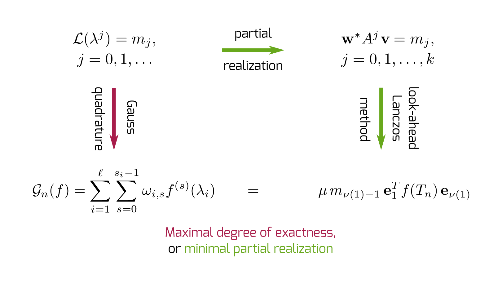
Figure 2: Visualization of the connections between the Gauss quadrature for linear functionals, minimal partial realization, and look-ahead Lanczos algorithm.

Figure 2 summarizes the connections between the Gauss quadrature for linear functionals, minimal partial realization, and look-ahead Lanczos algorithm. On the right-hand side, the triplet $({\mathbf{w}},A,{\mathbf{v}})$ is a partial realization matching the first $k+1$ elements of the sequence of complex numbers $m_{0},m_{1},\dots$ . A minimal partial realization can be obtained applying the look-ahead Lanczos algorithm to the matrix $A$ and the vectors $\mathbf{v},\mathbf{w}$ (this is also connected with the concept of model reduction, see, e.g., (LieStrBook13, , Chapter 3, in particular Section 3.9)). Notice that the Lanczos algorithm applied to the partial realization (6.2) is related to the Berlekamp-Massey algorithm Ber68 ; Mass69 (see Kun77 , GraLin83 , and BoLeLu92 ). On the left-hand side, the sequence $m_{0},m_{1},\dots$ determines the linear functional $\mathcal{L}:\mathcal{P}\rightarrow\mathbb{C}$ by defining its moments. The functional $\mathcal{L}$ can be approximated by a Gauss quadrature. Among all the Gauss quadratures exact on $\mathcal{P}_{k}$, there is one with the minimal number of nodes $n$ (counting the multiplicities). Such quadrature can be written in the matrix form

$$\mathcal{G}_{n}(f)=\mu\,m_{\nu{(1)}-1}\,\mathbf{e}_{1}^{T}f(T_{n})\,\mathbf{e}_{\nu{(1)}},$$

i.e., it corresponds to the minimal partial realization matching $m_{0},\dots,m_{k}$.

In Sections 6 and 7, we discussed the correspondence between the incurable breakdown in the look-ahead Lanczos algorithm and the minimal realization of an infinite sequence of complex numbers (and to the unique Gauss quadrature exact for every polynomial). This connection led us to a new proof for the Mismatch Theorem 7.3.

- (1) Antoulas, A.C.: Approximation of Large-Scale Dynamical Systems, Advances in Design and Control, vol. 6. SIAM, Philadelphia, PA (2005). With a foreword by Jan C. Willems
- (2) Bai, Z.: Error analysis of the Lanczos algorithm for the nonsymmetric eigenvalue problem. Math. Comp. 62(205), 209–226 (1994). DOI 10.2307/2153404. URL https://doi.org/10.2307/2153404
- (3) Bai, Z., Day, D.M., Ye, Q.: ABLE: an adaptive block Lanczos method for non-Hermitian eigenvalue problems. SIAM J. Matrix Anal. Appl. 20(4), 1060–1082 (1999). DOI 10.1137/S0895479897317806. URL https://doi.org/10.1137/S0895479897317806
- (4) Beckermann, B.: Complex Jacobi matrices. J. Comput. Appl. Math. 127, 17–65 (2001)
- (5) Berlekamp, E.R.: Algebraic coding theory. McGraw-Hill Book Co., New York-Toronto, Ont.-London (1968)
- (6) Boley, D.L., Lee, T.J., Luk, F.T.: The Lanczos algorithm and Hankel matrix factorization. Linear Algebra Appl. 172, 109–133 (1992). DOI 10.1016/0024-3795(92)90022-3. URL https://doi.org/10.1016/0024-3795(92)90022-3. Second NIU Conference on Linear Algebra, Numerical Linear Algebra and Applications (DeKalb, IL, 1991)
- (7) Brezinski, C.: Padé-type approximation and general orthogonal polynomials. Internat. Ser. Numer. Math. Birkhäuser (1980)
- (8) Brezinski, C.: Computational aspects of linear control, Numerical Methods and Algorithms, vol. 1. Kluwer Acad. Publ., Dordrecht (2002). DOI 10.1007/978-1-4613-0261-2. URL https://doi.org/10.1007/978-1-4613-0261-2
- (9) Brezinski, C., Redivo Zaglia, M., Sadok, H.: Avoiding breakdown and near-breakdown in Lanczos type algorithms. Numer. Algorithms 1(3), 261–284 (1991). DOI 10.1007/BF02142326. URL http://dx.doi.org/10.1007/BF02142326
- (10) Brezinski, C., Redivo Zaglia, M., Sadok, H.: A breakdown-free Lanczos type algorithm for solving linear systems. Numer. Math. 63(1), 29–38 (1992). DOI 10.1007/BF01385846. URL http://dx.doi.org/10.1007/BF01385846
- (11) Bultheel, A., Van Barel, M.: Linear Algebra, Rational Approximation and Orthogonal Polynomials, Stud. Comput. Math., vol. 6. North-Holland Publishing Co., Amsterdam (1997)
- (12) Chebyshev, P.: Sur les fractions continues (1855). Reprinted in Oeuvres I, 11 (Chelsea, New York, 1962), pp. 203–230
- (13) Chebyshev, P.: Le développement des fonctions à une seule variable (1859). Reprinted in Oeuvres I, 19 (Chelsea, New York, 1962), pp. 501–508
- (14) Chihara, T.S.: On quasi-orthogonal polynomials. Proc. Amer. Math. Soc. 8, 765–767 (1957). DOI 10.2307/2033295. URL https://doi.org/10.2307/2033295
- (15) Chihara, T.S.: An Introduction to Orthogonal Polynomials, Mathematics and its Applications, vol. 13. Gordon and Breach Science Publishers, New York (1978)
- (16) Christoffel, E.B.: Über die Gaußische Quadratur und eine Verallgemeinerung derselben. J. Reine Angew. Math. 55, 61–82 (1858). Reprinted in Gesammelte mathematische Abhandlungen I (B. G. Teubner, Leipzig, 1910), pp. 65–87
- (17) Cullum, J., Kerner, W., Willoughby, R.A.: A generalized nonsymmetric Lanczos procedure. Comput. Phys. Commun. 53(1), 19–48 (1989). DOI 10.1016/0010-4655(89)90146-X. URL http://www.sciencedirect.com/science/article/pii/001046558990146X
- (18) Cullum, J., Willoughby, R.A.: A practical procedure for computing eigenvalues of large sparse nonsymmetric matrices. In: North-Holland Mathematics Studies, vol. 127, pp. 193–240. Elsevier (1986)
- (19) Cybenko, G.: An explicit formula for Lanczos polynomials. Linear Algebra Appl. 88, 99–115 (1987)
- (20) Day, D.M.: Semi-duality in the two-sided Lanczos algorithm. Ph.D. thesis, University of California, Berkeley (1993). URL http://gateway.proquest.com/openurl?url_ver=Z39.88-2004&rft_val_fmt=info:ofi/fmt:kev:mtx:dissertation&res_dat=xri:pqdiss&rft_dat=xri:pqdiss:9430449
- (21) Day, D.M.: An efficient implementation of the nonsymmetric Lanczos algorithm. SIAM J. Matrix Anal. Appl. 18(3), 566–589 (1997). DOI 10.1137/S0895479895292503. URL https://doi.org/10.1137/S0895479895292503
- (22) Draux, A.: Polynômes Orthogonaux Formels, Lecture Notes in Math. , vol. 974. Springer-Verlag, Berlin (1983)
- (23) Draux, A.: On quasi-orthogonal polynomials. J. Approx. Theory 62(1), 1–14 (1990). DOI 10.1016/0021-9045(90)90042-O. URL https://doi.org/10.1016/0021-9045(90)90042-O
- (24) Draux, A.: Formal orthogonal polynomials revisited. Applications. Numer. Algorithms 11(1), 143–158 (1996). DOI 10.1007/BF02142493. URL https://doi.org/10.1007/BF02142493
- (25) Draux, A.: On quasi-orthogonal polynomials of order . Integral Transforms Spec. Funct. 27(9), 747–765 (2016). DOI 10.1080/10652469.2016.1197922. URL https://doi.org/10.1080/10652469.2016.1197922
- (26) Fenu, C., Martin, D., Reichel, L., Rodriguez, G.: Block Gauss and Anti-Gauss Quadrature with Application to Networks. SIAM J. Matrix Anal. Appl. 34(4), 1655–1684 (2013). DOI 10.1137/120886261. URL https://doi.org/10.1137/120886261
- (27) Freund, R.W.: The Look-Ahead Lanczos Process for Large Nonsymmetric Matrices and Related Algorithms. In: M.S. Moonen, G.H. Golub, B.L.R. de Moor (eds.) Linear Algebra for Large Scale and Real-Time Applications, NATO ASI Series, vol. 232, pp. 137–163. Kluwer Acad. Publ., Dordrecht (1993)
- (28) Freund, R.W., Gutknecht, M.H., Nachtigal, N.M.: An implementation of the look-ahead Lanczos algorithm for non-Hermitian matrices. SIAM J. Sci. Comput. 14(1), 137–158 (1993)
- (29) Freund, R.W., Hochbruck, M.: Gauss Quadratures Associated With the Arnoldi Process and the Lanczos Algorithm. In: M.S. Moonen, G.H. Golub, B.L.R. de Moor (eds.) Linear Algebra for Large Scale and Real-Time Applications, NATO ASI Series, vol. 232, pp. 377–380. Kluwer Acad. Publ., Dordrecht (1993)
- (30) Freund, R.W., Zha, H.: A look-ahead algorithm for the solution of general Hankel systems. Numer. Math. 64(1), 295–321 (1993). DOI 10.1007/BF01388691. URL https://doi.org/10.1007/BF01388691
- (31) Gantmacher, F.R.: On the algebraic analysis of Krylov’s method of transforming the secular equation. Trans. Second Math. Congress II, 45–48 (1934). In Russian. Title translation as in GanBook59
- (32) Gantmacher, F.R.: The Theory of Matrices. Vols. 1, 2. Chelsea Publishing Co., New York (1959)
- (33) Gautschi, W.: A survey of Gauss-Christoffel quadrature formulae. In: E. B. Christoffel (Aachen/Monschau, 1979), pp. 72–147. Birkhäuser, Basel (1981)
- (34) Gautschi, W.: Orthogonal Polynomials: Computation and Approximation. Numer. Math. Sci. Comput. . Oxford University Press, New York (2004)
- (35) Gautschi, W.: Numerical Analysis. Birkhäuser Boston (2011). URL https://books.google.it/books?id=-fgjJF9yAIwC
- (36) Gilbert, E.: Controllability and observability in multivariable control systems. SIAM J. Control 1, 128–151 (1963)
- (37) Golub, G.H., Meurant, G.: Matrices, Moments and Quadrature with Applications. Princeton Ser. Appl. Math. Princeton University Press, Princeton, NJ (2010)
- (38) Golub, G.H., Van Loan, C.F.: Matrix Computations, fourth edn. Johns Hopkins Stud. Math. Sci. Johns Hopkins University Press, Baltimore, MD (2013)
- (39) Gragg, W.B.: Matrix interpretations and applications of the continued fraction algorithm. Rocky Mountain J. Math. 4, 213–225 (1974)
- (40) Gragg, W.B., Lindquist, A.: On the partial realization problem. Linear Algebra Appl. 50, 277–319 (1983)
- (41) Günnel, A., Herzog, R., Sachs, E.: A note on preconditioners and scalar products in Krylov subspace methods for self-adjoint problems in Hilbert space. Elect. Trans. Numer. Anal. 41, 13–20 (2014)
- (42) Guo, H., Renaut, R.A.: Estimation of for large-scale unsymmetric matrices. Numer. Linear Algebra Appl. 11(1), 75–89 (2004). DOI 10.1002/nla.334. URL http://dx.doi.org/10.1002/nla.334
- (43) Gutknecht, M.H.: A completed theory of the unsymmetric Lanczos process and related algorithms. I. SIAM J. Matrix Anal. Appl. 13(2), 594–639 (1992)
- (44) Gutknecht, M.H.: A completed theory of the unsymmetric Lanczos process and related algorithms. II. SIAM J. Matrix Anal. Appl. 15(1), 15–58 (1994)
- (45) Gutknecht, M.H.: The Lanczos Process and Padé approximation. In: Proceedings of the Cornelius Lanczos International Centenary Conference (Raleigh, NC, 1993), pp. 61–75. SIAM, Philadelphia, PA (1994)
- (46) Heinig, G., Jankowski, P.: Kernel structure of block Hankel and Toeplitz matrices and partial realization. Linear Algebra Appl. 175, 1–30 (1992). DOI 10.1016/0024-3795(92)90299-P. URL https://doi.org/10.1016/0024-3795(92)90299-P
- (47) Heinig, G., Rost, K.: Algebraic methods for Toeplitz-like matrices and operators, Operator Theory: Advances and Applications, vol. 13. Birkhäuser Verlag, Basel (1984). DOI 10.1007/978-3-0348-6241-7. URL https://doi.org/10.1007/978-3-0348-6241-7
- (48) Hestenes, M.R., Stiefel, E.: Methods of conjugate gradients for solving linear systems. J. Research Nat. Bur. Standards 49, 409–436 (1952)
- (49) Higham, N.J.: Functions of Matrices. Theory and Computation. SIAM, Philadelphia, PA (2008)
- (50) Ho, B., Kalman, R.E.: Effective construction of linear state-variable models from input/output functions. at-Automatisierungstechnik 14(1-12), 545–548 (1966)
- (51) Hochbruck, M.: The Padé Table and its Relation to Certain Numerical Algorithms. Habilitation thesis, Universität Tübingen (1996)
- (52) Householder, A.S., Bauer, F.L.: On certain methods for expanding the characteristic polynomial. Numer. Math. 1, 29–37 (1959)
- (53) Iohvidov, I.S.: Hankel and Toeplitz matrices and forms. Birkhäuser, Boston, Mass. (1982). Algebraic theory, Translated from the Russian by G. Philip A. Thijsse, With an introduction by I. Gohberg
- (54) Kailath, T.: Linear systems. Prentice-Hall, Inc., Englewood Cliffs, N.J. (1980). Prentice-Hall Information and System Sciences Series
- (55) Kalman, R.E.: Canonical structure of linear dynamical systems. Proc. Nat. Acad. Sci. U.S.A. 48, 596–600 (1962)
- (56) Kalman, R.E.: Mathematical description linear systems. SIAM J. Control 1, 152–192 (1963)
- (57) Kalman, R.E.: On partial realizations, transfer functions, and canonical forms. Acta Polytech. Scand. Math. Comput. Sci. Ser. 31, 9–32 (1979)
- (58) Kautský, J.: Matrices related to interpolatory quadratures. Numer. Math. 36(3), 309–318 (1980/81). DOI 10.1007/BF01396657. URL http://dx.doi.org/10.1007/BF01396657
- (59) Krall, H.L., Sheffer, I.M.: Differential equations of infinite order for orthogonal polynomials. Annali di Matematica Pura ed Applicata 74(1), 135–172 (1966). DOI 10.1007/BF02416454. URL https://doi.org/10.1007/BF02416454
- (60) Kung, S.Y.: Multivariable and multidimensional systems: analysis and design. Ph.D. thesis, Stanford University, Stanford (1977)
- (61) Kwon, K.H., Littlejohn, L.L.: Classification of classical orthogonal polynomials. J. Korean Math. Soc 34(4), 973–1008 (1997)
- (62) Lanczos, C.: An iteration method for the solution of the eigenvalue problem of linear differential and integral operators. J. Research Nat. Bur. Standards 45, 255–282 (1950)
- (63) Lanczos, C.: Solution of systems of linear equations by minimized iterations. J. Research Nat. Bur. Standards 49, 33–53 (1952)
- (64) Liesen, J., Strakoš, Z.: Krylov subspace methods: principles and analysis. Numer. Math. Sci. Comput. Oxford University Press, Oxford (2013)
- (65) Lorentzen, L., Waadeland, H.: Continued Fractions with Applications, Stud. Comput. Math., vol. 3. North-Holland Publishing Co., Amsterdam (1992)
- (66) Malék, J., Strakoš, Z.: Preconditioning and the Conjugate Gradient Method in the Context of Solving PDEs:. SIAM Spotlights. SIAM, Philadelphia (2015). URL https://books.google.it/books?id=aWDxBQAAQBAJ
- (67) Massey, J.L.: Shift-register synthesis and decoding. IEEE Trans. Information Theory IT-15, 122–127 (1969)
- (68) Milovanović, G.V., Cvetković, A.S.: Complex Jacobi Matrices and quadrature rules. Filomat 17, 117–134 (2003). URL http://www.jstor.org/stable/43998655
- (69) Moore, B.C.: Principal component analysis in linear systems: controllability, observability, and model reduction. IEEE Trans. Automat. Control 26(1), 17–32 (1981)
- (70) Nachtigal, N.M.: A look-ahead variant of the Lanczos algorithm and its application to the quasi-minimal residual method for non-Hermitian linear systems. Ph.D. thesis, Massachusetts Institute of Technology, Cambridge (1991)
- (71) Paige, C.C., Panayotov, I., Zemke, J.P.M.: An augmented analysis of the perturbed two-sided Lanczos tridiagonalization process. Linear Algebra Appl. 447, 119–132 (2014). DOI 10.1016/j.laa.2013.05.009. URL https://doi.org/10.1016/j.laa.2013.05.009
- (72) Parlett, B.N.: Reduction to tridiagonal form and minimal realizations. SIAM J. Matrix Anal. Appl. 13(2), 567–593 (1992)
- (73) Parlett, B.N., Taylor, D.R., Liu, Z.A.: A look-ahead Lanczos algorithm for unsymmetric matrices. Math. Comp. 44(169), 105–124 (1985). DOI 10.2307/2007796. URL http://dx.doi.org/10.2307/2007796
- (74) Piñar, M., Ramírez, V.: Matrix interpretation of formal orthogonal polynomials for nondefinite functionals. J. Comput. Appl. Math. 18(3), 265–277 (1987). DOI 10.1016/0377-0427(87)90001-X. URL http://dx.doi.org/10.1016/0377-0427(87)90001-X
- (75) Pozza, S., Pranić, M.S., Strakoš, Z.: Gauss quadrature for quasi-definite linear functionals. IMA J. Numer. Anal. 37(3), 1468–1495 (2017). DOI 10.1093/imanum/drw032. URL http://dx.doi.org/10.1093/imanum/drw032
- (76) Pozza, S., Pranić, M.S., Strakoš, Z.: The Lanczos algorithm and complex Gauss quadrature. Electron. Trans. Numer. Anal. 50, 1–19 (2018)
- (77) Pozza, S., Strakoš, Z.: Algebraic description of the finite Stieltjes moment problem. Linear Algebra Appl. 561, 207–227 (2019). DOI 10.1016/j.laa.2018.09.026. URL https://doi.org/10.1016/j.laa.2018.09.026
- (78) Riesz, M.: Sur le problème des moments. Troisième Note. Ark. Mat. Fys 17(16), 1–52 (1923)
- (79) Rutishauser, H.: Beiträge zur Kenntnis des Biorthogonalisierungs-Algorithmus von Lanczos. Z. Angew. Math. Physik 4, 35–56 (1953)
- (80) Saad, Y.: Iterative Methods for Sparse Linear Systems, second edn. SIAM, Philadelphia, PA (2003)
- (81) Stieltjes, T.J.: Recherches sur les fractions continues. Ann. Fac. Sci. Toulouse Sci. Math. Sci. Phys. 8(4), J. 1–122 (1894). Reprinted in Oeuvres II (P. Noordhoff, Groningen, 1918), pp. 402–566. English translation Investigations on continued fractions in Thomas Jan Stieltjes, Collected Papers, Vol. II (Springer-Verlag, Berlin, 1993), pp. 609–745
- (82) Strakoš, Z.: Model reduction using the Vorobyev moment problem. Numer. Algorithms 51(3), 363–379 (2009). DOI 10.1007/s11075-008-9237-0. URL http://dx.doi.org/10.1007/s11075-008-9237-0
- (83) Szegö, G.: Orthogonal Polynomials, Amer. Math. Soc. Colloq. Publ., vol. XXIII. American Mathematical Society, New York (1939)
- (84) Taylor, D.R.: Analysis of the look ahead Lanczos algorithm. Ph.D. thesis, University of California, Berkeley (1982)
- (85) Tong, C.H., Ye, Q.: Analysis of the finite precision bi-conjugate gradient algorithm for nonsymmetric linear systems. Math. Comp. 69(232), 1559–1575 (2000). DOI 10.1090/S0025-5718-99-01171-0. URL https://doi.org/10.1090/S0025-5718-99-01171-0
- (86) Vorobyev, Y.V.: Methods of Moments in Applied Mathematics. Translated from the Russian by Bernard Seckler. Gordon and Breach Science Publishers, New York (1965)
- (87) Wilkinson, J.H.: The Algebraic Eigenvalue Problem. Monographs on Numerical Analysis. The Clarendon Press Oxford University Press, New York (1988). 1st ed. published 1963