On the Benefits of Populations on the Exploitation Speed of Standard Steady-State Genetic Algorithms

Abstract.

It is generally accepted that populations are useful for the global exploration of multi-modal optimisation problems. Indeed, several theoretical results are available showing such advantages over single-trajectory search heuristics. In this paper we provide evidence that evolving populations via crossover and mutation may also benefit the optimisation time for hillclimbing unimodal functions. In particular, we prove bounds on the expected runtime of the standard ($\mu$+1) GA for OneMax that are lower than its unary black box complexity and decrease in the leading constant with the population size up to $\mu=O(\sqrt{\log n})$. Our analysis suggests that the optimal mutation strategy is to flip two bits most of the time. To achieve the results we provide two interesting contributions to the theory of randomised search heuristics: 1) A novel application of drift analysis which compares absorption times of different Markov chains without defining an explicit potential function. 2) The inversion of fundamental matrices to calculate the absorption times of the Markov chains. The latter strategy was previously proposed in the literature but to the best of our knowledge this is the first time is has been used to show non-trivial bounds on expected runtimes.

1. Introduction

Populations in evolutionary and genetic algorithms are considered crucial for the effective global optimisation of multi-modal problems. For this to be the case, the population should be sufficiently diverse such that it can explore multiple regions of the search space at the same time (Friedrich et al., 2009). Also, if the population has sufficient diversity, then it considerably enhances the effectiveness of crossover for escaping from local optima. Indeed the first proof that crossover can considerably improve the performance of GAs relied on either enforcing diversity by not allowing genotypic duplicates or by using unrealistically small crossover rates for the Jump function (Jansen and Wegener, 2002). It has been shown several times that crossover is useful to GAs using the same, or similar, diversity enhancing mechanisms for a range of optimisation problems including shortest path problems (Doerr et al., 2012), vertex cover (Neumann et al., 2011), colouring problems inspired by the Ising model (Sudholt, 2005) and computing input output sequences in finite state machines (Lehre and Yao, 2011).

These examples provide considerable evidence that, by enforcing the necessary diversity, crossover makes GAs effective and often superior to applying mutation alone. However, rarely it has been proven that the diversity mechanisms are actually necessary for GAs, or to what extent they are beneficial to outperform their mutation-only counterparts rather than being applied to simplify the analysis. Recently, some light has been shed on the power of standard genetic algorithms without diversity over the same algorithms using mutation alone. Dang et al. showed that the plain ($\mu$+1) GA is at least a linear factor faster than its ($\mu$+1) EA counterpart at escaping the local optimum of Jump (Dang et al., 2018). Sutton showed that the same algorithm with crossover if run sufficiently many times is a fixed parameter tractable algorithm for the closest string problem while without crossover it is not (Sutton, 2018). Lengler provided an example of a class of unimodal functions to highlight the robustness of the crossover based version with respect to the mutation rate compared to the mutation-only version i.e., the ($\mu$+1) GA is efficient for any mutation rate $c/n$ while the ($\mu$+1) EA requires exponential time as soon as approx. $c>2.13$ (Lengler, 2018). In all three examples the population size has to be large enough for the results to hold, thus providing evidence of the importance of populations in combination with crossover.

Recombination has also been shown to be very helpful at exploitation if the necessary diversity is enforced through some mechanism. In the (1+($\lambda,\lambda$)) GA such diversity is achieved through large mutation rates. The algorithm can optimise the well-known OneMax function in sublogarithmic time with static offspring population sizes $\lambda$ (Doerr and Doerr, 2015b), and in linear time with self-adaptive values of $\lambda$ (Doerr and Doerr, 2015a). Although using a recombination operator, the algorithm is still basically a single-trajectory one (i.e., there is no population). More realistic steady-state GAs that actually create offspring by recombining parents have also been analysed for OneMax. Sudholt showed that ($\mu$+$\lambda$) GAs are twice as fast as their mutation-only version (i.e., no recombination) for OneMax if diversity is enforced artificially i.e., genotype duplicates are preferred for deletion (Sudholt, 2017). He proved a runtime of $(e/2)n\ln n+O(n)$ versus the $en\ln n+O(n)$ function evaluations required by any standard bit mutation-only evolutionary algorithm for OneMax and any other linear function (Witt, 2012). If offspring are identical to their parents it is not necessary to evaluate the quality of their solution. When the unnecessary queries are avoided, the expected runtime of the GA using artificial diversity from (Sudholt, 2017) is bounded above by $(1+o(1))0.850953n\ln{n}$ (Pinto and Doerr, 2018). Hence, it is faster than any unary (i.e., mutation-only) unbiased   black-box search heuristic (Lehre and Witt, 2012)

On one hand, the enforced artificiality in the last two results considerably simplifies the analysis. On the other hand, the power of evolving populations for effective optimisation cannot be appreciated. Since the required diversity to make crossover effective is artificially enforced, the optimal population size is 2 and larger populations provide no benefits. Corus and Oliveto showed that the standard ($\mu$+1) GA without diversity is still faster than mutation-only ones by proving an upper bound on the runtime of $(3/4)en\ln n+O(n)$ for any $3<\mu<o(\log n/\log\log n)$ (Corus and Oliveto, 2017). A result of enforcing the diversity in (Sudholt, 2017) was that the best GA for the problem only used a population of size 2. However, even though this artificiality was removed in  (Corus and Oliveto, 2017), a population of size 3 was sufficient to get the best upper bound on the runtime achievable with their analysis. Overall, their analysis does not indicate any tangible benefit towards using a population larger than $\mu=3$. Thus, rigorously showing that populations are beneficial for GAs in the exploitation phase has proved to be a non-trivial task.

In this paper we provide a more precise analysis of the behaviour of the population of the ($\mu$+1) GA for OneMax. We prove that the standard ($\mu$+1) GA is at least $60\%$ faster than the same algorithm using only mutation. We also prove that the GA is faster than any unary unbiased black-box search heuristic if offspring with identical genotypes to their parents are not evaluated. More importantly, our upper bounds on the expected runtime decrease with the population size up to $\mu=o(\sqrt{\log n})$, thus providing for the first time a natural example where populations evolved via recombination and mutation optimise faster than unary unbiased heuristics.

2. Problem Definition and Our Results

2.1. The Genetic Algorithm

The ($\mu$+1) GA is a standard steady-state GA which samples a single new solution at every generation (Eiben and Smith, 2003; Sarma and Jong, 1997). It keeps a population of the $\mu$ best solutions sampled so far and at every iteration selects two solutions from the current population uniformly at random with replacement as the parents. The recombination operator then picks building blocks from the parents to create the offspring solution. For the case of pseudo-Boolean functions $f:\{0,1\}^{n}\rightarrow\mathbb{R}$, the most frequently used recombination operator is uniform crossover which picks the value of each bit position $i\in[n]$ from one parent or the other uniformly at random (i.e., from each parent with probability 1/2) (Eiben and Smith, 2003). Then, an unbiased unary variation operator, which is called the mutation operator, is applied to the offspring solution before it is added to the population. The most common mutation operator is the standard bit-mutation which independently flips each bit of the offspring solution with some probability $c/n$ (Witt, 2012). Finally, before moving to the next iteration, one of the solutions with the worst fitness value is removed from the population. For the case of maximisation the ($\mu$+1) GA is defined in Algorithm 1. The runtime of Algorithm 1 is the number of function evaluations until a solution which maximises the function $f$ is sampled for the first time. If every offspring is evaluated, then the runtime is equal to the value of the variable $t$ in Alg. 1 when the optimal solution is sampled. However, if the fitness of offspring which are identical to their parents are not evaluated, then the runtime is smaller than $t$. We will first analyze the former scheme and then adapt the result to the latter.

1 $P_{1}\leftarrow\mu\textrm{ individuals, uniformly at random from }\{0,1\}^{n}$;

2 $t\leftarrow\mu$;

3 repeat

4       Select $x,y\in P_{t}$ uniformly at random with replacement ;

5       $z\leftarrow$ uniform crossover$(x,y)$;

6       $z\leftarrow mutate(z)$;

7       $P_{t+1}\leftarrow P_{t}\cup\{z\}$;

8       Remove the element with lowest fitness from $P_{t+1}$, breaking ties at random;

9       $t\leftarrow t+1$;

10until optimum is found;

Algorithm 1 ($\mu$+1) GA (Eiben and Smith, 2003; Sarma and Jong, 1997)

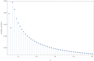
Figure 1. The leading constant from the second statement of Theorem 3.1 versus the population size. The best leading constant achievable by any unary unbiased algorithm is $1$.

2.2. The Optimisation Problem

Given a secret bitstring $z\in\{0,1\}^{n}$, $\text{\sc OneMax}_{z}(x):=\{i\in[n]|z_{i}=x_{i}\}$ returns the number of bits on which a candidate solution $x\in\{0,1\}^{n}$ matches $z$ (Witt, 2012). The optimisation time (synonymously, runtime) is defined by the number of queries to the function required by an algorithm to minimise the Hamming distance between the candidate solution and the hidden bitstring $z$.

2.3. Our Results

In this paper we prove the following results.

Informal 0.

The expected runtime for the ($\mu$+1) GA (with unbiased mutations and population size $\mu=o(\sqrt{\log{n}})$ to optimise the OneMax function is

1. $E[T]\leq(1+o(1))n\ln{n}\cdot\gamma_{1}(\mu,p_{0},p_{1},p_{2}),$ if offspring identical to their parents are not evaluated for their quality is known and $p_{0}$, $p_{1}$, and $p_{2}$ are respectively the probabilities that zero, one or two bits are flipped, [Theorem 3.1, Section 3]

2. $E[T]\leq(1+o(1))n\ln{n}\cdot\gamma_{2}(\mu,c),$ if the quality of all offspring is evaluated and using standard bit mutation with rate $c/n$, $c\in\Theta(1)$, [Corollary 3.2, Section 3]

where $\gamma_{1}$ and $\gamma_{2}$ are decreasing functions of the population size $\mu$.

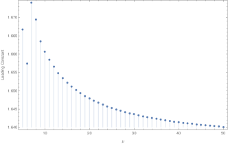
Figure 2. The leading constant from the first statement of Corollary 3.2 versus the population size. The best mutation-only variant has a the leading constant of $e\approx 2.71$.

The above two statements are very general as they provide upper bounds on the expected runtime of the ($\mu$+1) GA for each value of the population size up to $\mu=o(\sqrt{\log{n}})$ and any unbiased mutation operator. The leading constants $\gamma_{1}$ and $\gamma_{2}$ in Statements 1 and 2 are plotted respectively in Fig. 1 and 2 for different population sizes using the $p_{0}$, $p_{1}$, $p_{2}$ and $c$ values which minimise the upper bounds. The result is significant particularly for the following three reasons (in order of increasing importance).

(1) The first statement shows how the genetic algorithm outperforms any unbiased mutation-only heuristic since the best expected runtime achievable by any algorithm belonging to such class is at least $n\ln n-cn\pm o(n)$  (Doerr et al., 2016). Given that the best expected runtime achievable with any search heuristic using only standard bit mutation is $(1+o(1))en\ln{n}$ (Witt, 2012), the second statement shows how by adding recombination a speed-up of 60% is achieved for the OneMax problem for any population size up to $\mu=o(\sqrt{\log{n}})$.

(2) Very few results are available proving constants in the leading terms of the expected runtime for randomised algorithms due to the considerable technical difficulties in deriving them. Exceptions exist such as the analyses of (Witt, 2012) and (Doerr et al., 2016) without which our comparative results would not have been achievable. While such precise results are gaining increasing importance in the theoretical computer science community, the available ones are related to more simple algorithms. This is the first time similar results are achieved concerning a much more complicated to analyse standard genetic algorithm using realistic population sizes and recombination.

(3) The preciseness of the analysis allows for the first time an appreciation of the surprising importance of the population for optimising unimodal functions  as our upper bounds on the expected runtime decrease as the population size increases. In particular as the problem size increases, so does the optimal size of the population (the best known runtime available for the ($\mu$+1) GA was of $(1+o(1))3/4en\ln n$ independent of the population size as long as it is greater than $\mu=3$ i.e., there were no evident advantages in using a larger population (Corus and Oliveto, 2017)). This result is in contrast to all previous analyses of simplified evolutionary algorithms for unimodal functions where the algorithmic simplifications, made for the purpose of making the analysis more accessible, caused the use of populations to be either ineffective or detrimental (Witt, 2006; Sudholt, 2017; Pinto and Doerr, 2018). Our upper bound of $\mu=o(\sqrt{\log{n}})$ is very close to the at most logarithmic population sizes typically recommended for monotone functions to avoid detrimental runtimes (Corus et al., 2017; Witt, 2006). We conjecture that the optimal population size is $\Theta(\log n^{1-\epsilon})$ for any constant $\epsilon>0$, which cannot be proven with our mathematical methods for technical reasons.

2.4. Proof Strategy

Our aim is to provide a precise analysis of the expected runtime of the ($\mu$+1) GA for optimising OneMax with arbitrary problem size $n$. Deriving the exact transition probabilities of the algorithm from all possible configurations to all others of its population is prohibitive. We will instead devise a set of $n$ Markov chains, one for each improvement the algorithm has to pessimistically make to reach the global optimum, which will be easier to analyse. Then we will prove that the Markov chains are slower to reach their absorbing state than the ($\mu$+1) GA is in finding the corresponding improvement.

In essence, our proof strategy consists of: (1) to identify suitable Markov chains, (2) to prove that the absorbing times of the Markov chains are larger than the expected improving times of the actual algorithm and (3) to bound the absorbing times of each Markov chain.

In particular, concerning point (2) we will first define a potential function which monotonically increases with the number of copies of the genotype with most duplicates in the population and then bound the expected change in the potential function at every iteration (i.e., the drift ) from below. Using the maximum value of the potential function and the minimum drift, we will bound the expected time until the potential function value drops to its minimum value for the first time. This part of the analyses is a novel application of drift analysis techniques (Lehre and Witt, 2014). In particular, rather than using an explicit distance function as traditionally occurs, we define the potential function to be equal to the conditional expected absorption time of the corresponding states of each Markov chain.

Concerning point (3) of our proof strategy, we will calculate the absorbing times of the Markov chains $M^{j}$ by identifying their fundamental matrices. This requires the inversion of tridiagonal matrices. Similar matrix manipulation strategies to bound the runtime of evolutionary algorithms have been previously suggested in the literature (He and Yao, 2003; Oliveto and Yao, 2011). However, all previous applications showed that the approach could only be applied to prove results that could be trivially achieved via simpler standard methods. To the best of our knowledge, this is the first time that the power of this long abandoned approach has finally been shown by proving non-trivial bounds on the expected runtime.

3. Main Result Statement

Our main result is the following theorem. The transition probabilities $p_{i,k}$ for $(i,k)\in[m]^{2}$ and $m:=\lceil\mu/2\rceil$ are defined in Definition 4.1 (Section 4.1) and are depicted in Figure 3.

Theorem 3.1.

The expected runtime for the ($\mu$+1) GA with $\mu=o(\sqrt{\log{n}})$ using an unbiased mutation operator $mutate(x)$ that flips $i$ bits with probability $p_{i}$ with $p_{0}\in\Omega(1)$ and $p_{1}\in\Omega(1)$ to optimise the OneMax function is:

1. $E[T]\leq(1+o(1))n\ln{n}\frac{1}{p_{1}+p_{2}\frac{2(1-\xi_{2})\mu}{(\mu+1)}}$ if the quality of each offspring is evaluated,

2. $E[T]\leq(1+o(1))n\ln{n}\frac{(1-p_{0})}{p_{1}+p_{2}\frac{2(1-\xi_{2})\mu}{(\mu+1)}}$ if the quality of offspring identical to their parents is not evaluated for their quality is known; and

$$\xi_{i}=\frac{p_{i-1,i-2}}{p_{i-1,m}+p_{i-1,i-2}+p_{i-1,i}(1-\xi_{i+1})}, \xi_{m}=\frac{p_{m-1,m-2}}{p_{m-1,m}+p_{m-1,m-2}}.$$

The recombination operator of the GA is effective only if individuals with different genotypes are picked as parents (i.e., recombination cannot produce any improvements if two identical individuals are recombined). However, more often than not, the population of the ($\mu$+1) GA consists only of copies of a single individual. When diversity is created via mutation (i.e., a new genotype is added to the population), it either quickly leads to an improvement or it quickly disappears. The bound on the runtime reflects this behaviour as it is simply a waiting time until one of two event happens; either the current individual is mutated to a better one or diversity emerges and leads to an improvement before it is lost.

The $\xi_{2}$ term in the runtime is the conditional probability that once diversity is created by mutation, it will be lost before reaching the next fitness level (an improvement). Naturally, $(1-\xi_{2})$ is the probability that a successful crossover will occur before losing diversity. The $(1-\xi_{2})$ factor increases with the population size $\mu$, which implies that larger populations have a higher capacity to maintain diversity long enough to be exploited by the recombination operator.

Note that setting $p_{i}:=0$ for all $i>2$ minimises the upper bound on the expected runtime in the second statement of Theorem 3.1 and reduces the bound to: $E[T]\leq(1+o(1))n\ln{n}(p_{1}+p_{2})/\left(p_{1}+p_{2}\frac{2\mu(1-\xi_{2})}{\mu+1}\right)$. Now, we can see the critical role that $\xi^{*}(\mu)=(1-\xi_{2})\mu/(\mu+1)$ plays in the expected runtime. For any population size which yields $\xi^{*}(\mu)\leq 1/2$, flipping only one bit per mutation becomes advantageous. The best upper bound achievable from the above expression is then $(1+o(1))n\ln{n}$ by assigning an arbitrarily small constant to $p_{0}$ and $p_{1}=1-p_{0}$. As long as $p_{0}=\Omega(1)$, when an improvement occurs, the superior genotype takes over the population quickly relative to the time between improvements. Since there are only one-bit flips, the crossover operator becomes virtually useless (i.e., crossover requires a Hamming distance of 2 between parents to create an improving offspring) and the resulting algorithm is a stochastic local search algorithm with a population. However, when $\xi^{*}(\mu)>1/2$ setting $p_{2}$ as large as possible provides the best upper bound. The transition for $\xi^{*}(\mu)$ happens between population sizes of 4 and 5. For populations larger than 5, by setting $p_{1}:=\epsilon/2$ and $p_{0}=:\epsilon/2$ to an arbitrarily small constant $\epsilon$ and setting $p_{2}=1-\epsilon$, we get the upper bound $E[T]\leq(1+o(1))(1+\epsilon)n\ln{n}\left(\mu+1\right)/\left(2\mu\left(1-\xi_{2}\right)\right)$, which is plotted for different population sizes in Figure 1.

A direct corollary to the main result is the upper bound for the classical ($\mu$+1) GA commonly used in evolutionary computation which applies standard bit mutation with mutation rate $c/n$ for which $p_{0}=(1-o(1))/e^{c}$, $p_{1}=(1-o(1))c/e^{c}$ and $p_{2}=(1-o(1))c^{2}/(2e^{c})$.

Corollary 3.2.

Let $\xi_{2}$ be as defined in Theorem 3.1. The expected runtime for the ($\mu$+1) GA with $\mu=o(\sqrt{\log{n}})$ using standard bit-mutation with mutation rate $c/n$, $c=\Theta(1)$ to optimise the OneMax function is:

1. $E[T]\leq(1+o(1))n\ln{n}\frac{e^{c}}{c+\frac{c^{2}\mu}{(\mu+1)}(1-\xi_{2})}$ if the quality of each offspring is evaluated,

2. $E[T]\leq(1+o(1))n\ln{n}\frac{(1-e^{-c})e^{c}}{c+\frac{c^{2}\mu}{(\mu+1)}(1-\xi_{2})}$ if the quality of offspring identical to their parents is not evaluated for their quality is known;

By calculating $\xi^{*}(\mu):=(1-\xi_{2})\mu/(\mu+1)$ for fixed values of $\mu$ we can determine values of $c$ (i.e., mutation rate) which minimise the leading constant of the runtime bound in Corollary 3.2. In Figure 2 we plot the leading constants in the first statement, minimised by picking the appropriate $c$ values for $\mu$ ranging from 5 to 50. All the values presented improve upon the upper bound on the runtime of $1.96n\ln{n}$ given in (Corus and Oliveto, 2017) for any $\mu\geq 3$ and $\mu=o(\log{n}/\log{\log{n}})$. All the upper bounds are less than $1.7n\ln{n}$ and clearly decrease with the population size, signifying an at least $60\%$ increase in speed compared to the $en\ln{n}\left(1-o\left(1\right)\right)$ lower bound for the same algorithm without the recombination operator.

Considering the leading constants in the second statement of Corollary 3.2, for all population sizes larger than 5, the upper bound for the optimal mutation rate is smaller than the theoretical lower bound on the runtime of unary unbiased black-box algorithms. For population sizes of 3 and 4, $\xi^{*}=1/3$ and the expression to be minimised is $(1-e^{-c})e^{c}/(c+c^{2}/3)$. For $c>0$, this expression has no minimum and is always larger than one. Thus, at least with our technique, a population of size 5 or larger is necessary to prove that the ($\mu$+1) GA outperforms stochastic local search and any other unary unbiased optimisation heuristic.

4. Analysis

Our main aim is to provide an upper bound on the expected runtime ($E[T]$) of the ($\mu$+1) GA defined in Algorithm 1 to maximise the OneMax function. W.l.o.g. we will assume that the target string $z$ of the $\text{\sc OneMax}_{z}$ function to be identified is the bitstring of all 1-bits since all the operators in the ($\mu$+1) GA are invariant to the bit-value (have no bias towards $0$s or $1$s). We will provide upper bounds on the expected value $E[T^{j}]$, where $T^{j}$ is the time until an individual with at least $j+1$ 1-bits is sampled for the first time given that the initial population consists of individuals with $j$ 1-bits (i.e., the population is at level $j$). Then, by summing up the values of $E[T^{j}]$ and the expected times for the whole population to reach $j+1$ 1-bits for $j\in\{1\ldots,,n-1\}$ we achieve a valid upper bound on the runtime of the ($\mu$+1) GA. Similarly to the analysis in (Corus and Oliveto, 2017), we will pessimistically assume that the algorithm is initialised with all individuals having just 0-bits, and that throughout the optimisation process at most one extra 1-bit is discovered at a time.

We will devise a Markov chain $M^{j}$ for each $j\in\{0,\ldots,n-1\}$ for which we can analyse the expected absorbing time $E[T_{i}^{j}]$ starting from state $S_{i}^{j}$. We will then prove that it is in expectation slower in reaching its absorbing state than the ($\mu$+1) GA is in finding an improvement given an initial population at level $j$. In particular, we will define a non-negative potential function on the domain of all possible configurations of a population at level $j$ or above. For any configuration at level $j$, we will refer to the genotype with the most copies in the population as the majority genotype and define the diversity of a population as the number of non-majority individuals in the population. Our potential function will be monotonically decreasing with the diversity. Moreover, we will assign the potential function a value of zero for all populations with at least one solution which has more than $j$ 1-bits. Then, we will bound the expected change in the potential function at every iteration (i.e., the drift) from below. Using the maximum value of the potential function and the minimum drift, we will derive a bound on the expected time until an improvement is found starting from a population at level $j$ with no diversity (i.e., all the solutions in the population are identical). While this upper bound will not provide an explicit runtime as a function of the problem size, it will allow us to conclude that the $E[T_{0}^{j}]\geq E[T^{j}]$. Thus, all that remains will be to bound the expected absorbing time of $M^{j}$ initialised at state $S_{0}^{j}$. We will obtain this bound by identifying the fundamental matrix of $M^{j}$. After establishing that the inverse of the fundamental matrix is a strongly diagonally dominant tridiagonal matrix, we will make use of existing tools in the literature for inverting such matrices and complete our proof.

4.1. Markov Chain Definition

Figure 3. The topology of Markov Chain $M^{j}$.

In this subsection we will present the Markov chains which we will use to model the behaviour of the ($\mu$+1) GA. Each Markov chain $M^{j}$ has $m:=\lceil\mu/2\rceil$ transient states ($S^{j}_{0},S^{j}_{1},\ldots,S^{j}_{m-1}$) and one absorbing state ($S^{j}_{m}$ ) with the topology depicted in Figure 3. The states $S_{i}^{j}$ represent the amount of diversity in the population. Hence, eg., $S_{1}^{j}$ refers to a population where all the individuals have $j$ 1-bits and all but one of them share the same genotype, while $S_{m-1}^{j}$ refers to a population where at most $m-1=\lceil\mu/2\rceil+1$ individuals are identical. Compared to the analysis presented in (Corus and Oliveto, 2017) that used Markov chains of only three states (i.e., no diversity, diversity, increase in 1-bits), $M^{j}$ allows to control the diversity in the population more precisely, thus to show that larger populations are beneficial to the optimisation process.

Definition 4.1.

Let $M_{j}$ be a Markov chain with $m:=\lceil\mu/2\rceil$ transient states ($S^{j}_{0},S^{j}_{1},\ldots,S^{j}_{m-1}$) and one absorbing state ($S^{j}_{m}$ ) with transition probabilities $p_{i,k}$ from state $S^{j}_{i}$ to state $S^{j}_{k}$ as follows:

$$p_{0,1} :=\frac{\mu}{(\mu+1)}\frac{2j(n-j)p_{2}}{n^{2}},\quad p_{0,m}:=\frac{(n-j)p_{1}}{n},$$

$$\quad p_{i,m} :=2\frac{i}{\mu}\frac{\mu-i}{\mu}\frac{p_{0}}{4}\quad\text{ if }i>0,$$

$$p_{1,2} :=p_{0}\left(\left(\frac{1}{\mu}\right)^{2}\frac{\mu-1}{\mu+1}+2\frac{1}{\mu}\frac{\mu-1}{\mu}\frac{1}{4}\frac{\mu-1}{\mu+1}\right),$$

$$p_{1,0} :=p_{0}\left(\left(\frac{\mu-1}{\mu}\right)^{2}+2\frac{1}{\mu}\frac{\mu-1}{\mu}\frac{1}{4}\right)\frac{1}{\mu+1},$$

$$p_{i,i+1} :=p_{0}\left(\left(\frac{i}{\mu}\right)^{2}\min{\left(\frac{\mu-i}{\mu+1},1/4\right)}+2\frac{i}{\mu}\frac{\mu-i}{\mu}\frac{1}{4}\frac{\mu-i}{\mu+1}\right)\quad$$

if $$m-1>i>1,$$

$$p_{i,i-1} :=p_{0}\left(\left(\frac{\mu-i}{\mu}\right)^{2}+2\frac{i}{\mu}\frac{\mu-i}{\mu}\frac{1}{4}+\left(\frac{i}{\mu}\right)^{2}\frac{1}{16}\right)\frac{i}{\mu+1}$$

if $$m>i>1,$$

$$p_{m,m} :=1,\quad p_{0,0}:=1-p_{0,1}-p_{0,m},$$

$$p_{m-1,m-1} :=1-p_{m-1,m-2}-p_{m-1,m},$$

$$p_{i,i} :=1-p_{i,i-1}-p_{i,i+1}-p_{i,m}\quad\text{ if }0<i<m-1,$$

$$p_{i,j} :=0\quad otherwise.$$

Now, we will point out the important characteristics of these transition probabilities. The transition probabilities, $p_{i,k}$, are set to be equal to provable bounds on the probabilities of the ($\mu$+1) GA with a population consisting of solutions with $j$ bits of gaining/losing diversity ($p_{i,i+1}$/$p_{i,i-1}$) and sampling a solution with more than $j$ 1-bits ($p_{i,m}$). In particular, upper bounds are used for the transition probabilities $p_{i,k}$ where $i<k$ and lower bounds are used for the transition probabilities $p_{i,k}$ where $i>k$. Note that greater diversity corresponds to a higher probability of two distinct individuals with $j$ 1-bits being selected as parents and improved via recombination (i.e., $p_{i,m}$ monotonically increases with $i$ and recombination is ineffective if $i=0$ and the improvement probability $p_{0,m}$ is simply the probability of increasing the number of 1-bits by mutation only. Thus, $p_{0,m}=\Theta(j/n)$ while $p_{i,m}=\Theta(i(\mu-i)/\mu^{2})$ when $i>0$. The first forward transition probability $p_{0,1}$ denotes the probability of the mutation operator of creating a different individual with $j$ 1-bits and the selection operator removing one of the majority individuals from the population. The other transition probabilities, $p_{i,i+1}$ and $p_{i,i-1}$ bound the probability that a copy of the minority solution or the majority solution is added to the population and that a member of the other species (minority/majority) is removed in the subsequent selection phase. All transition probabilities except $p_{0,1}$ and $p_{0,m}$ are independent of $j$ and referred to in the theorem statements without specifying $j$.

4.2. Validity of the Markov Chain Model

In this subsection we will present how we establish that $M^{j}$ is a pessimistic representation of Algorithm 1 initialised with a population of $\mu$ identical individuals at level $j$. In particular, we will show that $E[T^{j}_{0}]$, the expected absorbing time starting from state $S_{0}^{j}$ is larger than $E[T^{j}]$. This result is formalised in the following lemma.

Lemma 4.2.

Let $E[T]$ be the expected runtime until the ($\mu$+1) GA with $\mu=o(\log{n}/\log{\log{n}})$ optimises the OneMax function and $E[T_{i}^{j}]$ (or $E[T_{i}]$ wherever $j$ is obvious) is the expected absorbing time of $M^{j}$ starting from state $S^{j}_{i}$. Then, $E[T]\leq o(n\log{n})+(1+o(1))\sum_{j=0}^{n-1}E[T_{0}^{j}]$.

We will use drift analysis (Lehre and Witt, 2014), a frequently used tool in the runtime analysis of evolutionary algorithms, to prove the above result. We will start by defining a potential function over the state space of Alg. 1 that maps states to the expected absorbing times of $M^{j}$. The minimum of the potential function will correspond to the state of Algorithm 1 which has sampled a solution with more than $j$ 1-bits and we will explicitly prove that the maximum of the potential function is $E[T^{j}_{0}]$. Then, we will show that the drift, i.e., the expected decrease in the potential function value in a single time unit (from time $t$ to $t+1$), is at least one. Using the maximum value of the potential function and the minimum drift, we will bound the runtime of the algorithm by the absorbing time of the Markov chain.

We will define our potential function over the domain of all possible population diversities at level $j$. We will refer to the genotype with the most copies in the population as the majority genotype and recall that the diversity, $D_{t}\in\{0,\ldots,\mu-1\}$, of a population $P_{t}$ is defined as the number of non-majority individuals in the population.

Definition 4.3.

The potential function value for level $j$, $g^{j}$ (or $g$ wherever $j$ is obvious), is defined as follows:

$$g^{j}(D_{t})=g^{j}_{t}=\begin{cases}E[T_{D_{t}}]&0\leq D_{t}<\lceil\mu/2\rceil-1\\ E[T_{\lceil\mu/2\rceil-1}]&\lceil\mu/2\rceil-1\leq D_{t}<\mu-1\\ 0&\exists x\in P_{t}\quad s.t.\quad\text{\sc OneMax}(x)>j\end{cases}$$

where $E[T_{i}^{j}]$ (denoted as $E[T_{i}]$ wherever $j$ is obvious) is the expected absorbing time of the Markov chain $M^{j}$ starting from state $S^{j}_{i}$.

The absorbing state of the Markov chain corresponds to a population with at least one individual with more than $j$ 1-bits, thus having potential function value (and expected absorbing time) equal to zero. The state $S_{0}^{j}$ corresponds to a population with no diversity. The following lemma formalises that the expected absorbing time gets larger as the initial states get further away from $\lceil\mu/2\rceil-1$. This property implies that the expected absorbing time from state $S_{0}^{j}$ constitutes an upper bound for the potential function $g^{j}$.

Lemma 4.4.

Let $E[T^{j}_{i}]$ be the expected absorbing time of Markov chain $M^{j}$ conditional on its initial state being $S_{i}^{j}$. Then, $\forall j\in\{0,\ldots,n-1\}$, $E[T^{j}_{i}]\geq E[T^{j}_{i-1}]$ for all $1\leq i\leq\lceil\mu/2\rceil$ and $g^{j}_{t}\leq E[T^{j}_{0}]$ $\quad\forall t>0$.

Now that the potential function is bounded from above, we will bound the drift $E[g_{t}-g_{t+1})|D_{t}=i]$. Due to the law of total expectation, the expected absorbing time, $E[T_{i}]$ satisfies $\sum_{j}p_{i,j}(E[T_{j}]-E[T_{i}])=1$ for any absorbing Markov chain at state $i$. Since $E[T_{i}]$ and $E[T_{j}]$ are the respective potentials of the states $S_{i}$ and $S_{j}$, the left hand side of the equation closely resembles the drift. Since the probabilities for $M^{j}$ are pessimistically set to underestimate the drift, the above equation allows us to formally prove the following:

Lemma 4.5.

For a population at level $j$, $E[g_{t}^{j}-g_{t+1}^{j}|D_{t}=i]\geq 1-o(1)$ for all $t>0$

Proof.

We will now show that $\Delta_{t}(i):=E[g_{t}-g_{t+1}|D_{t}=i]$, the expectation of the difference between the potential function values of population $P_{t}$ and $P_{t+1}$, is larger than one for all $i$.

When there is no diversity in the population (i.e., $D_{t}=0$) the only way to increase the diversity is to introduce it during a mutation operation. A non-majority individual is obtained when one of the $n-j$ 0-bits and one of the $j$ 1-bits are flipped while no other bits are touched. Then one of the majority individuals must be removed from the population during the selection phase.This event has probability at least $p_{2}\cdot 2\cdot\frac{(n-j)}{n}\frac{j}{n}\frac{\mu}{\mu+1}=p_{0,1}.$ Another way to change the potential function value is to create an improved individual with the mutation operator. In order to improve a solution it is sufficient to pick one of $n-j$ 1-bits and flip no other bits. This event has the probability at least $p_{1}\cdot\frac{(n-j)}{n}=p_{0,m}.$Thus, we can conclude that when $D_{t}=0$, the drift is at least $p_{0,m}(T_{0})+p_{0,1}(T_{0}-T_{1})$. We can observe through the law of total expectation for the state $S^{j}_{0}$ of Markov chain $M^{j}$ that this expression for the drift when $D_{t}=0$ is larger than one.

For $D_{t}>0$, we will condition the drift on whether the picked parents are both majority individuals $\mathcal{E}_{1}$, are both minority individuals with the same genotype $\mathcal{E}_{2}$, are a pair that consists of one majority and one minority individual $\mathcal{E}_{3}$, or they are both minority individuals with different genotypes $\mathcal{E}_{4}$.

Let $\mathcal{E}^{*}$ be the event that the population $P_{t}$ consists of two genotypes with Hamming distance two. Then,

$$\mathbb{P}\{\mathcal{E}_{1}|\mathcal{E}^{*}\}=\mathbb{P}\{\mathcal{E}_{1}|\overline{\mathcal{E}^{*}}\}=\left(\frac{\mu-i}{\mu}\right)^{2}$$

$$\mathbb{P}\{\mathcal{E}_{2}|\mathcal{E}^{*}\}=\mathbb{P}\{\mathcal{E}_{2}|\overline{\mathcal{E}^{*}}\}+\mathbb{P}\{\mathcal{E}_{4}|\overline{\mathcal{E}^{*}}\}=\left(\frac{i}{\mu}\right)^{2}$$

(1) $$\mathbb{P}\{\mathcal{E}_{3}|\mathcal{E}^{*}\}=\mathbb{P}\{\mathcal{E}_{3}|\overline{\mathcal{E}^{*}}\}=2\frac{i}{\mu}\frac{\mu-i}{\mu};\quad\mathbb{P}\{\mathcal{E}_{4}|\mathcal{E}^{*}\}=0$$

Note that when there are more than two genotypes in the population, the event of picking any two non-majority individuals is divided into two separate cases of picking identical minority individuals and picking two different minority individuals. Obviously, the sum of the probabilities of these two cases is equal to the probability of picking two minority individuals when there are only two genotypes (one majority and one minority) in the population.

Restricting ourselves to $\Delta_{t}^{i>0}$, the drift conditional on $i>0$, the law of total expectation states:

$$\Delta_{t}^{i>0} =\mathbb{P}\{\mathcal{E}^{*}\}\sum_{i=1}^{4}\left(\mathbb{P}\{\mathcal{E}_{i}|\mathcal{E}^{*}\}\left(\Delta_{t}^{i>0}|\mathcal{E}_{i},\mathcal{E}^{*}\right)\right)+$$

$$+ (1-\mathbb{P}\{\mathcal{E}^{*}\})\sum_{i=1}^{4}\left(\mathbb{P}\{\mathcal{E}_{i}|\overline{\mathcal{E}^{*}}\}\left(\Delta_{t}^{i>0}|\mathcal{E}_{i},\overline{\mathcal{E}^{*}}\right)\right)$$

We can rearrange the above expression using the probabilities from Eq 4.2

$$\Delta_{t}^{i>0} \geq\left(\frac{\mu-i}{\mu}\right)^{2}\left(\Delta_{t}^{i>0}|\mathcal{E}_{1}\right)+\left(\frac{i}{\mu}\right)^{2}\min{\left(\left(\Delta_{t}^{i>0}|\mathcal{E}_{2}\right),\left(\Delta_{t}^{i>0}|\mathcal{E}_{4}\right)\right)}$$

$$+ 2\frac{\mu-i}{\mu}\frac{i}{\mu}\left(\Delta_{t}^{i>0}|\mathcal{E}_{3}\right)$$

We will now write the law of total expectation for state $i$ for our Markov chain $M^{j}$:

$$1=p_{i,i+1}(E[T_{i}]-E[T_{i+1}])+p_{i,i-1}(E[T_{i}]-E[T_{i-1}])+p_{i,m}E[T_{i}]$$

We will then substitute the probabilities in the law of total expectation with the values from Definition 4.1,

$$1 =p_{0}\left(\left(\frac{i}{\mu}\right)^{2}\min{\left(\frac{\mu-i}{\mu+1},1/4\right)}+2\frac{i}{\mu}\frac{\mu-i}{\mu}\frac{1}{4}\frac{\mu-i}{\mu+1}\right)(E[T_{i}]-E[T_{i+1}])$$

$$+p_{0}\left(\left(\frac{\mu-i}{\mu}\right)^{2}+2\frac{i}{\mu}\frac{\mu-i}{\mu}\frac{1}{4}+\left(\frac{i}{\mu}\right)^{2}\frac{1}{16}\right)\frac{i}{\mu+1}(E[T_{i}]-E[T_{i-1}])$$

$$+\left(2\frac{i}{\mu}\frac{\mu-i}{\mu}\frac{1}{4e^{c}}\right)E[T_{i}]$$

Finally, we will rearrange the above expression into the terms with the probabilities of events $\mathcal{E}_{i}$ as multiplicative factors

$$1 =\left(\frac{\mu-i}{\mu}\right)^{2}p_{0}\frac{i}{\mu+1}(E[T_{i}]-E[T_{i-1}])$$

$$+\left(\frac{i}{\mu}\right)^{2}p_{0}\bigg{(}\min{\left(\frac{\mu-i}{\mu+1},1/4\right)}(E[T_{i}]-E[T_{i+1}])$$

$$+\frac{1}{16}\frac{i}{\mu+1}(E[T_{i}]-E[T_{i-1}])\bigg{)}$$

$$+2\frac{i}{\mu}\frac{\mu-i}{\mu}p_{0}\bigg{(}\frac{1}{4}\frac{\mu-i}{\mu+1}(E[T_{i}]-E[T_{i+1}])$$

(2) $$+\frac{1}{4}\frac{i}{\mu+1}(E[T_{i}]-E[T_{i-1}])+\frac{E[T_{i}]}{4}\bigg{)}$$

We will refer to the first, second and third line of the Eq 2 as the $\mathcal{E}_{1}$, $\mathcal{E}_{2}$ and $\mathcal{E}_{3}$ term respectively. We will show that for each term, the conditional drift is larger than the term without the multiplicative factor.

When two majority individuals are selected as parents ($\mathcal{E}_{1}$), we pessimistically assume that improving to the next level and increasing the diversity has zero probability. Losing the diversity requires that no bits are flipped during mutation and that a minority individual will be removed from the population. The probability that no bits are flipped is $p_{0}$. Thus we can show that: $\Delta_{t}^{i>0}|\mathcal{E}_{1}\geq p_{0}\big{(}E[T_{i}]-E[T_{i-1}]\big{)}\frac{i}{\mu+1}$.

This bound is obviously the same as the $\mathcal{E}_{1}$ term of Eq 2 without the parent selection probability.

When two minority individuals are selected as parents($\mathcal{E}_{2}$ or $\mathcal{E}_{4}$), if they are identical ($\mathcal{E}_{2}$) then it is sufficient that the mutation does not flip any bits which occurs with probability $p_{0}$ and that a majority individual is removed from the population (with probability $(\mu-i)/\mu$). Thus, the probability of increasing the diversity is $p_{0}\times(\mu-i)/\mu$ and the probability of creating a majority individual is ${\mathcal{O}(1/n)}$ since it is necessary to flip at least one particular bit position: $\Delta_{t}^{i>0}|\mathcal{E}_{2}\geq p_{0}\frac{\mu-i}{\mu}(E[T_{i}]-E[T_{i+1}])$

However, if the two minority individuals have a Hamming distance of $2d\geq 2$ (i.e., $\mathcal{E}_{4}$), then in order to create another minority individual at the end of the crossover operation it is necessary that the crossover picks exactly $d$ 1-bits and $d$ 0-bits among $2d$ bit positions where they differ. There are $\binom{2d}{d}$ different ways that this can happen and the probability that any particular outcome of crossover is realised is $2^{-2d}$. One of those outcomes though, might be the majority individual and if that is the case the diversity can decrease afterwards. However, while the Hamming distance between the minority individuals can be $2d=2$, obtaining a majority individual by recombining two minority individuals requires at least four specific bit positions to be picked correctly during crossover and thus does not occur with probability greater than $1/16$. On the other hand, when two different minority individuals are selected as parents, there is at least a $\frac{1-\binom{2d}{d}2^{-2d}}{2}\geq 1/4$ probability that the crossover will result in an individuals with more 1-bits and then with probability $p_{0}$ the mutation will not flip any bits.

$$\Delta_{t}^{i>0}|\mathcal{E}_{4}\geq p_{0}\bigg{[}\left(\binom{2d}{d}-1\right)2^{-2d}\frac{\mu-i}{\mu+1}(E[T_{i}]-E[T_{i+1}])+$$

$$+\left(\min\left(\frac{1}{16},2^{-2d}\right)+{\mathcal{O}(1/n)}\right)\frac{i}{\mu+1}(E[T_{i}]-E[T_{i-1}])+\frac{1}{4}E[T_{i}]\bigg{]}$$

$$\geq\left(1-o(1)\right)\cdot p_{0}\bigg{[}\min\left(\frac{1}{16},2^{-2d}\right)\frac{i}{\mu+1}(E[T_{i}]-E[T_{i-1}])+\frac{E[T_{i}]}{4}\bigg{]}$$

Note that the $\mathcal{E}_{2}$ term of Eq 2 multiplied with a factor of $(1-o(1))$ is smaller than both conditional drifts multiplied with the parent selection probability $(i/\mu)^{2}$. Finally, we will consider the drift conditional on event $\mathcal{E}_{3}$, the case when one minority and one majority individual are selected as parents. We will further divide this event into two subcases. In the first case the Hamming distance $2d$ between the minority and the majority individual is exactly two ($d=1$). Then, the probabilities that crossover creates a copy of the minority individual, a copy of the majority individual or a new individual with more 1-bits are all equal to $1/4$. Thus, the conditional drift is $(\Delta_{t}^{i>0}|\mathcal{E}_{3},d=1)$

$$\geq \frac{p_{0}}{4}\left(\frac{i}{\mu+1}(E[T_{i}]-E[T_{i-1}])+\frac{\mu-i}{\mu+1}(E[T_{i}]-E[T_{i+1}])+E[T_{i}]\right).$$

However, when $d>1$, the drift is more similar to the case of $\mathcal{E}_{3}$ where the probabilities of creating copies of either the minority of the majority diminish with larger $d$ while larger $d$ increases the probability of creating an improved individual. More precisely, the drift is

$$(\Delta_{t}^{i>0}|\mathcal{E}_{3},d>1)\geq p_{0}\bigg{[}\left(\binom{2d}{d}-1\right)2^{-2d}\frac{\mu-i}{\mu+1}(E[T_{i}]-E[T_{i+1}])$$

$$+\left(2^{-2d}+{\mathcal{O}(1/n)}\right)\frac{i}{\mu+1}(E[T_{i}]-E[T_{i-1}])+(\frac{1-\binom{2d}{d}2^{-2d}}{2})E[T_{i}]\bigg{]}$$

$$\geq p_{0}\bigg{(}\left(2^{-2d}+{\mathcal{O}(1/n)}\right)\frac{i}{\mu+1}(E[T_{i}]-E[T_{i-1}])$$

$$+(\frac{1-\binom{2d}{d}2^{-2d}}{2})E[T_{i}]\bigg{)}$$

$$\geq p_{0}\left(\left(\frac{1}{16}+{\mathcal{O}(1/n)}\right)\frac{i}{\mu+1}(E[T_{i}]-E[T_{i-1}])+\frac{15}{32}E[T_{i}]\right)$$

$$\geq\left(1-o(1)\right)\cdot p_{0}\left(\frac{1}{16}\frac{i}{\mu+1}(E[T_{i}]-E[T_{i-1}])+\frac{15}{32}E[T_{i}]\right)$$

Since $(E[T_{i}]-E[T_{i-1}])$ is negative and $E[T_{i}]>E[T_{i}]-E[T_{i+1}]$, $(\Delta_{t}|\mathcal{E}_{3},d>1)\geq(\Delta_{t}|\mathcal{E}_{3},d=1)$. Now, finally we can observe that $(\Delta_{t}|\mathcal{E}_{3},d=1)$ multiplied with $2i(\mu-i)/\mu^{2}$ is larger than the $\mathcal{E}_{3}$ term in Eq 2 multiplied with a factor of $(1-o(1))$.

We have now shown piece by piece that the conditional drifts are larger than the corresponding terms in the right hand side of Eq 2 up to small order terms, and thus established that $\Delta_{t}\geq(1-o(1))$ for all $t>0$. Since we have previously shown that $g^{j}_{t}\leq T_{0}^{j}$, we can now apply Theorem 6.1 to obtain $E[T^{j}]\leq(1+o(1))E[T_{0}^{j}]$.

Once an individual with $j+1$ 1-bits is sampled for the first time it takes ${\mathcal{O}(\mu\log{\mu})}$ iterations before the whole population consists of individuals with at least $j+1$ 1-bits (Sudholt, 2017; Corus and Oliveto, 2017). If the population size is in the order of $o(\log{n}/\log{\log{n}})$, then the total number of iterations where there are individuals with different fitness values in the population is in the order of $o(n\log{n})$. Since $j\in\{0,1,\ldots,n-1\}$, we can establish that $E[T]\leq o(n\log{n})+\sum_{j=0}^{n-1}E[T^{j}]\leq o(n\log{n})+(1+o(1))\sum_{j=0}^{n-1}E[T_{0}^{j}]$. ∎

With the potential function bounded from above by Lemma 4.4 and the drift bounded from below by Lemma 4.5, we can use the additive drift theorem from (Lehre and Witt, 2014) to bound $E[T^{j}]$ by $E[T_{0}^{j}]$. By summing over all levels, we get the bound stated in Lemma 4.2 on the expected runtime of Algorithm 1.

4.3. Markov Chain Absorption Time Analysis

In the previous subsection we stated in Lemma 4.2 that we can bound the absorbing times of the Markov chains $M^{j}$ to derive an upper bound on the runtime of Algorithm 1. In this subsection we use mathematical tools developed for the analysis of Markov chains to provide such bounds on the absorbing times.

The absorbing time of a Markov chain starting from any initial state $i$ can be derived by identifying its fundamental matrix. Let the matrix $Q$ denote the transition probabilities between the transient states of the Markov chain $M^{j}$. The fundamental matrix of $M^{j}$ is defined as $N:=(I-Q)^{-1}$ where $I$ is the identity matrix. The most important characteristic of the fundamental matrix is that when it is multiplied by a column vector of ones, the product is a vector holding $E[T^{j}_{i}]$, the expected absorbing times conditional on the initial state $i$ of the Markov chain. Since, Lemma 4.2 only involves $T_{0}^{j}$, we are only interested in the entries of the first row of $N=[n_{ik}]$. However, inverting the matrix $I-Q$ is not always a straightforward task. Fortunately, $I-Q=[a_{ik}]$ has characteristics that allow bounds on the entries of its inverse. Its entries are related to the transition probabilities of $M^{j}$ as follows:

(3) $$a_{11} =1-p_{0,0}=p_{0,1}+p_{0,m}$$

(4) $$a_{mm} =1-p_{m-1,m-1}=p_{m-1,m-2}+p_{m-1,m}$$

$$a_{ii} =1-p_{i-1,i-1}=p_{i-1,i-2}+p_{i-1,i}+p_{i-1,m}$$

(5) $$\forall i\in\{2,...,m-1\}$$

(6) $$a_{ik} =-p_{i-1,k-1}\quad\forall i,k\in\{1,\ldots,m\}\wedge i\neq k$$

Observe that $I-Q$ is a tridiagonal matrix, in the sense that all non-zero elements of $I-Q$ are either on the diagonal or adjacent to it. Moreover, the diagonal entries $a_{ii}$ of $I-Q$ are in the form $1-p_{i-1,i-1}$, which is equal to the sum of all transition probabilities out of state $i-1$. Since the other entries on row $i$ are transition probabilities from state $i-1$ to adjacent states, we can see that $|a_{ii}|>\sum_{i\neq k}a_{ik}$. The matrices where $|a_{ii}|>\sum_{i\neq k}a_{ik}$ holds are called strongly diagonally dominant (SDD). Since $I-Q$ is SDD, according to Lemma 2.1 in (Li et al., 2010), it holds for the fundamental matrix $N$ for all $i\neq k$ that, $|n_{i,k}|\leq|n_{k,k}|\leq\left(|a_{k,k}|\left(1-\frac{\sum_{l\neq j}|a_{l,k}|}{|a_{k,k}|}\right)\right)^{-1}\leq\left(|a_{k,k}|-\sum_{l\neq j}|a_{l,k}|\right)^{-1}$.

In our particular case, the above inequality implies that $|n_{1,k}|\leq 1/p_{k-1,m}$. For any population with diversity, there is a probability in the order of ${\mathcal{O}(1/\mu)}$ to select one minority and one majority individual and a constant probability that their offspring will have more 1-bits than the current level. Considering $m={\mathcal{O}(\mu)}$, $E[T_{0}^{j}]=\sum_{k=1}^{m}n_{1,k}<n_{1,1}+\sum_{k=2}^{m}\frac{1}{p_{k-1,m}}\leq n_{1,1}+{\mathcal{O}(\mu^{2})}.$ We note here that the ${\mathcal{O}(\mu^{2})}$ factor in the above expression creates the condition $\mu=o(\sqrt{\log{n}})$ on the population size for our main results. We will now bound the term $n_{1,1}$ from above to establish our upper bound using the following theorem:

Theorem 4.6 (Direct corollary to Corollary 3.2 in (Li et al., 2010)).

$A$ is an $m\times m$ tridiagonal non-singular SDD matrix such that $a_{i,k}\leq 0$ for all $i\neq k$, $A^{-1}=[n_{i,k}]$ exists and $n_{i,k}\geq 0$ for all $i,k$, then $n_{1,1}=1/(a_{1,1}+a_{1,2}\xi_{2})$, $\xi_{i}=a_{i,i-1}/(a_{i,i}+a_{i,i+1}\xi_{i+1})$, and $\xi_{m}=a_{m,m-1}/a_{m,m}$.

In order to use Theorem 4.6, we need to satisfy its conditions. We can easily see that non-diagonal entries of the original matrix $I-Q$ are non-positive and use Theorem 3.1 in (Li et al., 2010) to show that $N=(I-Q)^{-1}$ has no negative entries. Thus, Theorem 4.6 yields:

Lemma 4.7.

With an initial population of size $\mu=o(\sqrt{\log{n}})$ at level $j$, the expected time $E[T^{j}]$ until an individual with $j+1$ 1-bits is sampled by the ($\mu$+1) GA for the first time is bounded from above as follows:

$$E[T^{j}_{0}]\leq\frac{n}{n-j}\frac{1}{p_{1}+\frac{2\mu p_{2}}{(\mu+1)}\frac{j}{n}(1-\xi_{2})}+o(\log{n})$$

$$\xi_{m}=\frac{p_{m-1,m-2}}{p_{m-1,m}+p_{m-1,m-2}}$$

$$\xi_{i}=\frac{p_{i-1,i-2}}{p_{i-1,m}+p_{i-1,i-2}+p_{i-1,i}(1-\xi_{i+1})}\quad\forall 1<i<m=\lceil\mu/2\rceil.$$

where $p_{i,k}$ are the transition probabilities of the Markov chain $M^{j}$.

The above bound on $E[T^{j}_{0}]$, together with Lemma 4.2, yields Theorem 3.1, our main result.

5. Conclusion

In this work, we have shown that the steady-state ($\mu$+1) GA optimises OneMax faster than any unary unbiased search heuristic. Providing precise asymptotic bounds on the expected runtime of standard GAs without artificial mechanisms that simplify the analysis has been a long standing open problem. We have derived bounds up to the leading term constants of the expected runtime. To achieve this result we show that a simplified Markov chain pessimistically represents the behaviour of the GA for OneMax. This insight about the algorithm/problem pair allows the derivation of runtime bounds for a complex multi-dimensional stochastic process. The analysis shows that as the number of states in the Markov chain (the population size) increases, so does the probability that diversity in the population is kept. Thus, larger populations increase the probability that recombination finds improved solutions quickly, hence reduce the expected runtime.

6. Appendix

6.1. Proof of Lemma 4.4

We will first show that $E[T^{j}]\leq(1+o(1))E[T_{0}^{j}]$ . In order to achieve this result, we will first establish that $g^{j}_{t}\leq E[T_{0}]\quad\forall t>0$ and then that $\Delta_{t}\geq 1-o(1)1\quad\forall t>0$. These two results will allow us to use Theorem 6.1 and conclude that $E[T^{j}]\leq(1+o(1))E[T_{0}^{j}]$. For the rest of the analysis of $E[T^{j}]$, we will drop the superscript of $E[T_{i}^{j}]$ and $g^{j}_{t}$.

Proof.

We are interested in $\max{(E[T_{0}],E[T_{1}],\ldots,E[T_{m}])}$ since these are the values that the potential function $g$ can have. According to the transition probabilities in Definition 4.1, $p_{i+1,m}\geq p_{i,m}$ for all $i$. Using this observation and the law of total expectation we can show that not only $\max{(E[T_{0}],E[T_{1}],\ldots,E[T_{m}])}=E[T_{0}]$ but also $E[T_{i-1}]\geq E[T_{i}]$ for all $i$. First, we will prove that $E[T_{m-2}]\geq E[T_{m-1}]$ by contradiction. Then, we will prove by induction that $E[T_{i-1}]\geq E[T_{i}]$ for all $i$. For this induction we will use $E[T_{m-2}]\geq E[T_{m-1}]$ as our basic step and we will prove by contradiction that if for all $j>i$ $E[T_{j-1}]\geq E[T_{j}]$ holds then $E[T_{i-1}]\geq E[T_{i}]$ must also hold.

If we use the law of total expectation for the absorbing time starting from state $0<i<m$, we obtain:

$$E[T_{i}]=p_{i,i+1}(E[T_{i+1}]+1)+p_{i,i-1}(E[T_{i-1}]+1)$$

$$+p_{i,m+1}+(1-p_{i,i+1}-p_{i,i-1}-p_{i,m})(E[T_{i}]+1)$$

This equation can be rearranged as follows:

$$1=p_{i,i+1}(E[T_{i}]-E[T_{i+1}])+p_{i,i-1}(E[T_{i}]-E[T_{i-1}])+p_{i,m}E[T_{i}]$$

For the special case of $i=m$, we have:

$$1=p_{m-1,m}(E[T_{m-1}])+p_{m-1,m-2}(E[T_{m-1}]-E[T_{m-2}])$$

If we introduce the allegedly contradictory assumption $E[T_{m-2}]<E[T_{m-1}]$, the above equation implies:

$$1>p_{m-1,m}(E[T_{m-1}])\implies\frac{1}{p_{m-2,m}}\geq\frac{1}{p_{m-1,m}}$$

$$>E[T_{m-1}]>E[T_{m-2}]$$

$$\implies\frac{1}{p_{m-2,m}}>E[T_{m-2}]$$

Given that $\frac{1}{p_{i,m}}>E[T_{i}]$ and $E[T_{i+1}]>E[T_{i}]$ the law of total expectation for $i$ implies:

$$1=p_{i,i+1}(E[T_{i}]-E[T_{i+1}])+p_{i,i-1}(E[T_{i}]-E[T_{i-1}])+p_{i,m}E[T_{i}]$$

$$1<p_{i,i+1}(E[T_{i}]-E[T_{i+1}])+p_{i,i-1}(E[T_{i}]-E[T_{i-1}])+1$$

$$0<p_{i,i-1}(E[T_{i}]-E[T_{i-1}])$$

$$E[T_{i-1}]<E[T_{i}]\implies\frac{1}{p_{i-1,m}}\geq\frac{1}{p_{i,m}}>E[T_{i}]>E[T_{i-1}]$$

Thus the allegedly contradictory claim $E[T_{m-1}]>E[T_{m-2}]$ induces over $i$ such that it implies $E[T_{1}]>E[T_{0}]$ and $1/p_{0,m}>E[T_{0}]$. We can now write the total law of expectation for $i=0$.

$$1=p_{0,1}(E[T_{0}]-E[T_{1}])+p_{0,m}E[T_{0}]$$

$$1<p_{0,1}(E[T_{0}]-E[T_{1}])+1$$

$$0<p_{0,1}(E[T_{0}]-E[T_{1}])$$

$$0>p_{0,1}$$

The last statement is a contradiction since a probability cannot be negative. This contradiction proves the initial claim $E[T_{m-2}]\geq E[T_{m-1}]$

We will now follow a similar route to prove that $E[T_{i-1}]\geq E[T_{i}]$ for all $i$. Given that for all $j>i$ $E[T_{j-1}]\geq E[T_{j}]$ holds, we will show that $E[T_{i}>E[T_{i-1}]$ creates a contradiction. We start with the law of total expectation for $E[T_{i}$:

$$1=p_{i,i+1}(E[T_{i}]-E[T_{i+1}])+p_{i,i-1}(E[T_{i}]-E[T_{i-1}])+p_{i,m}E[T_{i}]$$

Our assumption “ $\forall j>i\quad E[T_{j}]\leq E[T_{j-1}]$” implies that $E[T_{i}]-E[T_{i+1}]\geq 0$, thus we obtain:

$$1>p_{i,i-1}(E[T_{i}]-E[T_{i-1}])+p_{i,m}E[T_{i}]$$

With our allegedly contradictory assumption $E[T_{i}]-E[T_{i-1}]>0$ we obtain:

$$1>p_{i,m}E[T_{i}]\implies\frac{1}{p_{i-1,m}}\geq\frac{1}{p_{i,m}}>E[T_{i}]>E[T_{i-1}]$$

We have already shown above that $1/p_{i-1,m}\geq 1/p_{i,m}>E[T_{i}]>E[T_{i-1}]$ can be induced over $i$ and implies $E[T_{1}]>E[T_{0}]$ and $1/p_{0,m}>E[T_{0}]$. Then we can conclude that:

(7) $$E[T_{i}]\geq E[T_{i+1}]\quad\forall 0\leq i\leq\lceil\mu/2\rceil-1.$$

The above conclusion implies that $E[T_{0}]$ is the largest value that our potential function can have and $E[T_{i}]-E[T_{i+1}]$ is non-negative for all $i$. ∎

6.2. Proof of Lemma 4.2

Here, we will use the following additive drift theorem from (Lehre and Witt, 2014),

Theorem 6.1 (Theorem 3 in (Lehre and Witt, 2014)).

Let $(X_{t})_{t\in\mathbb{N}_{0}}$, be a stochastic process, adapted to a filtration $(\mathcal{F}_{t})_{t\in\mathbb{N}_{0}}$, over some state space $S\subseteq\{0\}\cup[x_{min},x_{max}]$, where $x_{min}\geq 0$. Let $g:\{0\}\cup[x_{min},x_{max}]\to\mathbb{R}^{\geq 0}$ be any function such that $g(0)=0,$ and $0<g(x)<\infty$ for all $x\in[x_{min},x_{max}]\setminus\{0\}$. Let $\mathcal{T}_{a}=\min\{t\mid X_{t}\leq a\}$ for $a\in\{0\}\cup[x_{min},x_{max}]$. If $E[g(X_{t})-g(X_{t+1})\,;\,{X_{t}\geq x_{min}}\mid\mathcal{F}_{t}]\geq\alpha_{\mathrm{u}}$ for some $\alpha_{\mathrm{u}}>0$ then $E[\mathcal{T}_{0}\mid X_{0}]\leq\frac{g(X_{0})}{\alpha_{\mathrm{u}}}$.

Proof of Lemma 4.2.

Since $\Delta_{t}\geq(1-o(1))$ from Lemma 4.5 and $g^{j}_{t}\leq E[T_{0}^{j}]$ from Lemma 4.4, we can apply Theorem 6.1 to obtain $E[T^{j}]\leq(1+o(1))E[T_{0}^{j}]$. Once an individual with $j+1$ 1-bits is sampled for the first time it takes ${\mathcal{O}(\mu\log{\mu})}$ iterations before the whole population consists of individuals with at least $j+1$ 1-bits (Corus and Oliveto, 2017). If the population size is in the order of $o(\log{n}/\log{\log{n}})$, then the total number of iterations where there are individuals with different fitness values in the population is in the order of $o(n\log{n})$. Since $j\in\{0,1,\ldots,n-1\}$, we can establish that

$$E[T]\leq o(n\log{n})+\sum_{j=0}^{n-1}E[T^{j}]\leq o(n\log{n})+(1+o(1))\sum_{j=0}^{n-1}E[T_{0}^{j}].$$

∎

6.3. Proof of Lemma 4.7

We made use of the following lemma to obtain .

(8) $$E[T_{0}^{j}]=\sum_{k=1}^{m}n_{1,k}<n_{1,1}+\sum_{k=2}^{m}\frac{1}{p_{k-1,m}}\leq n_{1,1}+{\mathcal{O}(\mu^{2})}.$$

Lemma 6.2 (Lemma 2.1 in (Li et al., 2010)).

Let $A$ be a SDD matrix, then $A^{-1}=[n_{ik}]$ exists and for any $i\neq k$,

$$|n_{ik}|\leq n_{kk}\frac{\sum\limits_{i\neq k}|a_{ik}|}{|a_{ii}|}\leq n_{kk}\leq\frac{1}{|a_{kk}|-\sum\limits_{l\neq k}|a_{kl}|}$$

In order to show that the entries of the fundamental matrix of $M^{j}$ are all non-negative, we will employ the following result.

Theorem 6.3 (Theorem 3.1 in (Li et al., 2010)).

If $A$ is a tridiagonal non-singular SDD matrix and $a_{i,i}>0$ then $A^{-1}=[n_{i,k}]$ exists and

• $sign(n_{i,i})=1$

• $sign(n_{i,k})=(-1)^{i+k}\prod^{i}_{l=k+1}a_{l,l-1},i>k$

• $sign(n_{i,k})=(-1)^{i+k}\prod^{k}_{l=i}a_{l,l+1},i<k$

Since the diagonal entries of $I-Q$ are strictly positive, according to Theorem 6.3 the diagonal entries of $N$ are also positive. The non-diagonal entries of $I-Q$ are all negative thus the series multiplication from Theorem 6.3 for $i>k$ reduces to $(-1)^{i+k+i-k}=(-1)^{2i}=1$. Similarly for the case $i<k$ the multiplication reduces to $(-1)^{i+k+k-i}=(-1)^{2k}=1$.

Proof.

Starting from Inequality 8 and applying Theorem 4.6 we obtain:

$$E[T_{0}^{j}] \leq n_{1,1}+{\mathcal{O}(\mu^{2})}\leq\frac{1}{a_{1,1}+a_{1,2}\xi_{2}}+{\mathcal{O}(\mu^{2})}$$

$$=\frac{1}{p_{0,m}+p_{0,1}(1-\xi_{2})}+{\mathcal{O}(\mu^{2})}$$

$$\leq \frac{1}{p_{0,m}+p_{0,1}(1-\xi_{2})}+{\mathcal{O}(\mu^{2})}$$

$$\leq\frac{1}{\frac{(n-j)p_{1}}{n}+\frac{\mu}{(\mu+1)}\frac{2j(n-j)p_{2}}{n^{2}}(1-\xi_{2})}+{\mathcal{O}(\mu^{2})}$$

$$=\frac{n}{n-j}\frac{1}{p_{1}+\frac{\mu}{(\mu+1)}\frac{2jp_{2}}{n}(1-\xi_{2})}+o(\log{n})$$

where we substitute $p_{0,1}$ and $p_{0,m}$ with their values declared in Definition 4.1. The definitions of $\xi_{i}$ and $\xi_{m}$ are obtained by simply substituting the matrix entries in Theorem 4.6 with their respective values from Equations 3 to 6. ∎

6.4. Proofs of main results

Proof of Theorem 3.1.

Combining Lemma 4.2 and Lemma 4.7 we obtain:

$$E[T] \leq o(n\log{n})+(1+o(1))\sum_{j=0}^{n-1}E[T^{j}]$$

(9) $$\leq o(n\log{n})+(1+o(1))\sum_{j=0}^{n-1}\left(\frac{n}{n-j}\frac{1}{p_{1}+\frac{\mu}{(\mu+1)}\frac{2jp_{2}}{n}(1-\xi_{2})}\right)$$

We will now divide the sum into two smaller sums:

$$\sum_{j=1}^{n}\frac{n}{n-j}\frac{1}{p_{1}+\frac{\mu}{(\mu+1)}\frac{2jp_{2}}{n}(1-\xi_{2})}$$

$$=\sum_{j=1}^{n-n/\sqrt{\log{n}}}\frac{n}{n-j}\frac{1}{p_{1}+\frac{\mu}{(\mu+1)}\frac{2jp_{2}}{n}(1-\xi_{2})}$$

$$+\sum_{j=n-n/\sqrt{\log{n}}+1}^{n}\frac{n}{n-j}\frac{1}{p_{1}+\frac{\mu}{(\mu+1)}\frac{2jp_{2}}{n}(1-\xi_{2})}$$

$$\leq{\mathcal{O}(n\sqrt{\log{n}})}+\frac{n}{p_{1}+\frac{2p_{2}\mu}{(\mu+1)}\left(1-\frac{1}{\sqrt{\log{n}}}\right)(1-\xi_{2})}\sum_{j=n-n/\sqrt{\log{n}}+1}^{n}\frac{1}{n-j}$$

$$\leq{\mathcal{O}(n\sqrt{\log{n}})}+\frac{n\ln{n}}{p_{1}+\frac{2p_{2}\mu}{(\mu+1)}\left(1-\frac{1}{\sqrt{\log{n}}}\right)(1-\xi_{2})}$$

We conclude the proof by substituting the sum in Eq 9 with the above expression.

$$E[T] \leq o(n\log{n})+(1+o(1))\left({\mathcal{O}(n\sqrt{\log{n}})}+\frac{n\ln{n}}{p_{1}+\frac{2p_{2}\mu}{(\mu+1)}\left(1-\frac{1}{\sqrt{\log{n}}}\right)(1-\xi_{2})}\right)$$

$$\leq o(n\log{n})+(1+o(1))\left({\mathcal{O}(n\sqrt{\log{n}})}+(1+o(1))\frac{n\ln{n}}{p_{1}+\frac{2p_{2}\mu}{(\mu+1)}(1-\xi_{2})}\right)$$

$$=(1+o(1))n\ln{n}\frac{1}{p_{1}+\frac{2p_{2}\mu}{(\mu+1)}(1-\xi_{2})}$$

The expressions for $\xi_{i}$ and $\xi_{m}$ come from Lemma 4.7 and proves the first statement.

For the second statement, we adapt the result for the variant of ($\mu$+1) GA which does not evaluate copies of either parents. When there is no diversity in the population the offspring is identical to the parent with probability $p_{0}$. Then, given that a fitness evaluation occurs, the probability of improvement via mutation is $p_{0,m}/(1-p_{0})$ and the probability that diversity is introduced is $p_{0,1}/(1-p_{0})$. The proof is identical to the proof of first statement, except for using probabilities $p^{*}_{0,m}=p_{0,m}/(1-p_{0})$ and $p^{*}_{0,1}=p_{0,1}/(1-p_{0})$ instead of $p_{0,1}$ and $p_{0,m}$ from Definition 4.1. Even if we pessimistically assume that a function evaluation occurs at every iteration when there is diversity in the population, we still get a $(1-p_{0})$ decrease in the leading constant. ∎

References

• (1)
• Corus etย al. (2017) D. Corus, D.ย C. Dang, A.ย V. Eremeev, and P.ย K. Lehre. 2017. Level-Based Analysis of Genetic Algorithms and Other Search Processes. IEEE Trans. on Evol. Comp. (2017). https://doi.org/10.1109/TEVC.2017.2753538
• Corus and Oliveto (2017) D. Corus and P.ย S. Oliveto. 2017. Standard Steady State Genetic Algorithms Can Hillclimb Faster than Mutation-only Evolutionary Algorithms. IEEE Trans. on Evol. Comp. (2017). https://doi.org/10.1109/TEVC.2017.2745715
• Dang etย al. (2018) D.-C. Dang, T. Friedrich, T. Kรถtzing, M.ย S. Krejca, P.ย K. Lehre, P.ย S. Oliveto, D. Sudholt, and A.ย M. Sutton. 2018. Escaping Local Optima Using Crossover with Emergent Diversity. IEEE Transactions on Evolutionary Computation 22, 3 (2018), 484โ€“497.
• Doerr and Doerr (2015a) B. Doerr and C. Doerr. 2015a. Optimal Parameter Choices Through Self-Adjustment: Applying the 1/5-th Rule in Discrete Settings. In Proc. of GECCO โ€™15. 1335โ€“1342.
• Doerr and Doerr (2015b) B. Doerr and C. Doerr. 2015b. A tight runtime analysis of the (1+($\lambda$, $\lambda$)) Genetic Algorithm on OneMax. In Proc. of GECCO โ€™15. 1423โ€“1430.
• Doerr etย al. (2016) B. Doerr, C. Doerr, and J. Yang. 2016. Optimal Parameter Choices via Precise Black-Box Analysis. In Proc. of GECCO โ€™16. 1123โ€“1130.
• Doerr etย al. (2012) Benjamin Doerr, Edda Happ, and Christian Klein. 2012. Crossover can provably be useful in evolutionary computation. Theoretical Computer Science 425, 0 (2012), 17โ€“33.
• Eiben and Smith (2003) A.ย E. Eiben and J.ย E. Smith. 2003. Introduction to evolutionary computing. Springer.
• Friedrich etย al. (2009) Tobias Friedrich, Pietroย S. Oliveto, Dirk Sudholt, and Carsten Witt. 2009. Analysis of Diversity-Preserving Mechanisms for Global Exploration. Evolutionary Computation 17, 4 (2009), 455โ€“476.
• He and Yao (2003) J. He and X. Yao. 2003. Towards an Analytic Framework for Analysing the Computation Time of Evolutionary Algorithms. Artificial Intelligence 145, 1-2 (2003), 59โ€“97.
• Jansen and Wegener (2002) Thomas Jansen and Ingo Wegener. 2002. The analysis of evolutionary algorithms-a proof that crossover really can help. Algorithmica 34, 1 (2002), 47โ€“66.
• Lehre and Witt (2012) P.ย K. Lehre and C. Witt. 2012. Black-Box Search by Unbiased Variation. Algorithmica 64, 4 (2012), 623โ€“642.
• Lehre and Witt (2014) P.ย K. Lehre and C. Witt. 2014. Concentrated Hitting Times of Randomized Search Heuristics with Variable Drift. In Proc. of ISAAC โ€™14. 686โ€“697.
• Lehre and Yao (2011) Perย Kristian Lehre and Xin Yao. 2011. Crossover can be constructive when computing unique inputโ€“output sequences. Soft Computing 15, 9 (2011), 1675โ€“1687. https://doi.org/10.1007/s00500-010-0610-2
• Lengler (2018) Johannes Lengler. 2018. A General Dichotomy of Evolutionary Algorithms on Monotone Functions. In Proceedings of Parallel Problem Solving from Nature (PPSN XV)). Springer, 3โ€“15.
• Li etย al. (2010) H.ย B. Li, T.ย Z. Huang, X.ย P. Liu, and H. Li. 2010. On the inverses of general tridiagonal matrices. Linear Algebra and Its Applications 433, 5 (2010), 965โ€“983.
• Neumann etย al. (2011) Frank Neumann, Pietroย S. Oliveto, Gรผnter Rudolph, and Dirk Sudholt. 2011. On the Effectiveness of Crossover for Migration in Parallel Evolutionary Algorithms. In Proceedings of the Genetic and Evolutionary Computation Conference (GECCO 2011). ACM Press, 1587โ€“1594.
• Oliveto and Yao (2011) P.ย S. Oliveto and X. Yao. 2011. Runtime analysis of evolutionary algorithms for discrete optimization. In Theory of Randomized Search Heuristics: Foundations and Recent Developments, B.ย Doerr and A.ย Auger (Eds.). World Scientific, 21.
• Pinto and Doerr (2018) E.ย C. Pinto and C. Doerr. 2018. A Simple Proof for the Usefulness of Crossover in Black-Box Optimization. In Parallel Problem Solving from Natureโ€“PPSN XV. 29โ€“41.
• Sarma and Jong (1997) J. Sarma and K.ย De Jong. 1997. Generation Gap Methods. In Handbook of evolutionary computation, T.ย Back, D.ย B Fogel, and Z.ย Michalewicz (Eds.). IOP Publishing Ltd.
• Sudholt (2005) Dirk Sudholt. 2005. Crossover is Provably Essential for the Ising Model on Trees. In Proceedings of the Genetic and Evolutionary Computation Conference (GECCO 2005). ACM Press, New York, New York, USA, 1161โ€“1167. https://doi.org/10.1145/1068009.1068202
• Sudholt (2017) D. Sudholt. 2017. How Crossover Speeds up Building Block Assembly in Genetic Algorithms. Evol. Comp. 25, 2 (2017), 237โ€“274.
• Sutton (2018) Andrew Sutton. 2018. Crossover can simulate bounded tree search on a fixed-parameter tractable optimization problem. In Proceedings of the Genetic and Evolutionary Computation Conference (GECCO 2018). ACM Press, 1531โ€“1538.
• Witt (2006) C. Witt. 2006. Runtime Analysis of the ( ยต+ 1) EA on Simple Pseudo-Boolean Functions. Evol. Comp. 14, 1 (2006), 65โ€“86.
• Witt (2012) C. Witt. 2012. Optimizing Linear Functions with Randomized Search Heuristics - The Robustness of Mutation. In Proc. of STACSโ€™12. 420โ€“431.