The first passage problem for stable linear delay equations perturbed by power law Lévy noise

Abstract

This article studies a linear scalar delay differential equation subject to small multiplicative power tail Lévy noise. We solve the first passage (the Kramers) problem with probabilistic methods and discover an asymptotic loss of memory in this non-Markovian system. Furthermore, the mean exit time increases as the power of the small noise amplitude, whereas the pre-factor accounts for memory effects. In particular, we discover a non-linear delay-induced exit acceleration due to a non-normal growth phenomenon. Our results are illustrated in the well-known linear delay oscillator driven by $\alpha$-stable Lévy flights.

Keywords: linear delay differential equation; $\alpha$-stable Lévy process; Lévy flights; heavy tails; first passage times; first exit; exit location.

AMS Subject Classification: 60H10; 60G51; 37A20; 60J60; 60J75; 60G52

1 Introduction and main results

The Kramers problem, that is, the escape time and location of a randomly excited deterministic dynamical system from the proximity of a stable state at small intensity was first stated in the context of physical chemistry in the seminal works of Arrhenius (1889), Eyring (1935) and Kramers (1940). The solution of this classical problem is ubiquitous nowadays and has given since crucial insight in many diverse areas such as statistical mechanics, insurance mathematics, climatic energy balance models and led to the discovery of more complex dynamical effects such as for instance stochastic resonance in complex systems Benzi et al. (1981, 1982, 1983).

In the mathematics literature, for Markovian systems such as of ordinary and partial differential equations with small Gaussian noise this problem was studied extensively with the help of large deviations theory which goes back to the seminal work by Cramér (1938) and later by Ventsel’ and Freidlin (1970); Vent-tsel’ (1976); Freidlin and Wentzell (2012), and in the recent years by Deuschel and Stroock (1989); Dembo and Zeitouni (1998); Barret et al. (2010); Bovier et al. (2002, 2004); Berglund and Gentz (2004, 2010, 2013); Cerrai and Roeckner (2004); Freidlin (2000). It is well-known that for $\varepsilon$-small Brownian diffusion in the potential well, the expected exit (excitation) time grows exponentially as

$$\mathbf{E}\tau^{\varepsilon}\sim\mathrm{e}^{\frac{\bar{V}}{\varepsilon^{2}}},$$ (1.1)

where $\bar{V}$ is proportional to the height of the potential barrier which has to be overcome by the particle. The exit location is determined by the deterministic energy minimizing path.

Penland and Ewald (2008), however, discusses “physical origins of stochastic forcing” and the trade off between Gaussian and non-Gaussian white and colored noises. Following their lines of reasoning, modelling with Lévy noises is the second best choice in complex systems, since they allow for richer effects such as local asymmetry and the presence of large bursts and jumps which are difficult to realize only with Gaussian influences. Furthermore Bódai and Franzke (2017) give evidence for physicality of Lévy noises in particular due to the predictability of fat-tail extremes while in the limit of small noise intensity, the (re-normalized) exit times are exponentially distributed and hence memoryless or unpredictable. Heavy-tailed noise has also been found present in many physical systems, for instance in works by Ditlevsen (1999a, b), Chen et al. (2019) and Gairing et al. (2017).

Due to a large variety of Lévy processes, i.e. stochastically continuous processes with independent stationary increments, there is no general Kramers’ theory for Lévy driven systems. Besides the well studied Gaussian case, a large deviations result for heavy tail Markovian processes was obtained by Godovanchuk (1982). For exponentially light jumps this question has been solved in one dimension by Imkeller et al. (2009, 2010). In addition, there is a large deviations theory for a special class of parameter dependent accelerated noise with exponentially light tails by Budhiraja et al. (2011) based on a variational representation. All these approaches yield exponential exit rates on the precise noise dependence. Further recent results on the first exit and metastability of Lévy driven systems in finite and infinite dimensions were obtained by Imkeller and Pavlyukevich (2006a); Pavlyukevich (2011); Debussche et al. (2013); Högele and Pavlyukevich (2013). It is worth mentioning that in the case of an overdamped particle subject to $\varepsilon$-small $\alpha$-stable noise, $\alpha\in(0,2)$, the expected exit time behaves polynomially

$$\mathbf{E}\tau^{\varepsilon}\sim\frac{\bar{V}}{\varepsilon^{\alpha}},$$ (1.2)

whereas the constant $\bar{V}$ has a very different interpretation. It is not the lowest height of any mountain pass the continuous Brownian diffusion path has to climb between different potential wells. Instead, it quantifies the tunelling effect of the “large” jumps that instantaneously overcome the (horizontal) distance between the deterministic stable state where the process lingers most of the time between such “large” jumps and the exterior of its domain of attraction.

In this article, we study such small heavy tailed perturbation of a beforehand non-Markovian dynamical system given as a linear delay differential equation. The simplest deterministic qualitative model of this kind is given by a linear retarded equation for the El Niño-Southern Oscillation phenomenon (ENSO) in Battisti and Hirst (1989):

$$\frac{\mathrm{d}}{\mathrm{d}t}X(t) =AX(t)+BX(t-r),$$ (1.3)

where $A$ is the sum of all processes that induce local changes in the SST, that is, the horizontal advection, thermal damping, mean and anomalous upwellings on the vertical temperature gradients. The coefficient $B$ subsumes the effects of the equatorial Kelvin waves. Positive $A$ means that the sum of effects of upwelling and thermal advection dominate the thermal damping, so that the temperature grows. However, negative values of $B$ can induce stable or periodic solutions. For instance, the parameter choice $A=2.2$, $B=3.8$, and a delay time of $r=0.5$ as in Battisti and Hirst (1989) leads to unstable oscillations with a period of approximately $3.0$ years and a growth rate of $1.1$ while Burgers (1999) argued that changing this to $A=2.4$, $B=-2.8$, and a delay time of $r=0.3$ leads to a period of approximately $4$ years and a decay rate $1.5$.

A more complex non-linear double-well model with an additional cubic term $-X^{3}$ was considered by Suarez and Schopf (1988), followed by a number of papers by e.g. Münnich et al. (1991); Tziperman et al. (1994); Ghil et al. (2008); Zaliapin and Ghil (2010).

Zabczyk (1987) studied the following delay equation perturbed by a small Brownian motion $\varepsilon W$

$$\mathrm{d}X^{\varepsilon}(t) =\mathcal{A}(X_{t}^{\varepsilon})\,\mathrm{d}t+\varepsilon\,\mathrm{d}W(t)$$ (1.4)

with a nonlinear Lipschitz continuous vector field $\mathcal{A}$. Applying a control theoretic approach to this equation he established a large deviations principle and showed that in analogy to the non-delay case discussed above the asymptotocs (1.1) holds true, however, with $\bar{V}$ being an abstract solution of a difficult delay control problem. Recently Lipshutz (2018) extended these results to the small noise SDDEs with multiplicative noise in the spirit of Freidlin and Wentzell (2012) and established the asymptotics of the first exit time of the type (1.1). Azencott et al. (2018) considered the retarded Gaussian delay equation as a Gaussian process and established the respective large deviations principle and the optimal exit paths with the help of the very elaborate Gaussian process theory. In Bao et al. (2016) the authors study delay systems perturbed by small accelerated Lévy noise with light tails in the spirit of Budhiraja et al. (2011). More on stochastic double-well systems can be found in Masoller (2002, 2003) and for Lévy noise also in Huang et al. (2011), where the authors study the asymptotics in the limit of small delay.

In this paper we study the first exit problem from an interval of the delay differential equation

$$\mathrm{d}X^{\varepsilon}(t) =\mathcal{A}X^{\varepsilon}_{t}\,\mathrm{d}t+\varepsilon F(X^{\varepsilon}_{t})\,\mathrm{d}Z(t),$$ (1.5)

with a general linear stable finite delay $\mathcal{A}$ perturbed by a small multiplicative heavy-tailed Lévy noise $\varepsilon Z$, including $\alpha$-stable but also more general weakly tempered perturbations. The phenomenological reason for our setting is that on the one hand we recover the rate (1.2), however, we detect a new non-normal growth effect in the factor $\bar{V}$, which we can calculate explicitly in the case of a retarded system (1.3). This effect accounts for the non-zero probability of small jump increments, which leads to an exit due to deterministic motion well after the occurrence of this jump and can be seen in the asymptotic distribution of the exit location, which in contrast to the non-delay case exhibits a point measure precisely on the boundary of the exit interval. It is easily seen that this effect vanishes if we send the memory depth to $0$. In other words, at first sight these results for non-Markovian systems appear surprising, however, since the delay time $r$ is negligible w.r.t. the exit time scale $\varepsilon^{-\alpha}$, the system behaviour is “almost” Markovian. Nevertheless the memory affects the prefactor in the asymptotics of the first exit time and the limiting distribution of the exit location.

The methodological reason for considering this equation is the adaption of the proof strategy by Godovanchuk (1982) and Imkeller et al. (2009) which is an elementary but very helpful application the Markov property which seems to be suitable for adaptation in different contexts of the physics literature. In addition, our setup covers generic non-degenerate potential gradient systems the linearized around their stable state.

A technical reason to study this particular problem is that in order to trace this effect we need a precise understanding of the deterministic dynamics. In particular, several important properties of this equation are readily given in the literature, such as existence, uniqueness of solutions and the invariant measure in Gushchin and Küchler (2000) and the segment Markov property in Reiß et al. (2006).

The article is organized as follows. After the general setup we present our main result in Theorem 2.2 followed by the discussion and examples, where we compare our results to the linear setting of Zabczyk (1987) and explicitly calculate the nonlinear growth factor. The rigorous proofs are postponed to the Mathematical Appendix and consist of two parts. In Section 4.1 we give general estimates on the deterministic relaxation dynamics and then on the stochastic perturbation. In Section 4.2 in we show a generic upper and a lower bound on the segment Markov process reducing the dynamics to four scenarios on a finite interval. This finite interval dynamics is treated in Section 4.3 for each of the cases what leads to the proof of the main result.

2 Object of Study and Results

2.1 General setup

The model under consideration is the following linear delay equation with finite memory $r>0$ perturbed by small Lévy noise defined below. For $r>0$ fixed and each $T>0$, we denote by $D[-r,T]$ the space of real valued right-continuous functions $\varphi\colon[-r,T]\to\mathbb{R}$ with left limits (the so-called càdlàg functions). Analogously we define the space $D[-r,\infty)$. For a function $\varphi\in D[-r,\infty)$ we we introduce the segment of $\varphi$ at time $t\geq 0$ as the function $\varphi_{t}(\cdot)\in D[-r,0]$ defined by $\varphi_{t}(s)=\varphi(t+s)$ for $s\in[-r,0]$. For a function $\varphi\in D[-r,0]$, we denote its uniform norm by $\|\varphi\|_{r}:=\sup_{t\in[-r,0]}|\varphi(t)|$.

Let $\mu$ be a finite, signed measure on the interval $[-r,0]$, so-called the memory measure. Consider the following underlying deterministic linear delay equation

$$x(t;\varphi) =\varphi(0)+\int_{0}^{t}\int_{[-r,0]}x(s+u;\varphi)\,\mu(\mathrm{d}u)\,\mathrm{d}s,\quad t\geq 0,$$ (2.1)

$$x(t;\varphi) =\varphi(t),\quad t\in[-r,0),$$

where $\varphi\in D[-r,0]$. It is well known that this equation has a unique solution which e.g. can be obtained by the method of steps as in Hale and Verduyn Lunel (1993). Similarly to the case of linear ODEs or PDEs, the solution $x(\cdot;\varphi)$ can be written down explicitly as a convolution integral, namely,

$$x(t;\varphi) =\varphi(0)x^{*}(t)+\int_{[-r,0]}\int_{u}^{0}x^{*}(t-s+u)\varphi(s)\,\mathrm{d}s\,\mu(\mathrm{d}u),\quad t\geq 0$$ (2.2)

$$x(t;\varphi) =\varphi(t),\quad t\in[-r,0),$$

where the fundamental solution $x^{*}(\cdot)$ is the unique solition of (2.1) with the initial segment $\varphi^{*}(t)=0$, $t\in[-r,0)$, and $\varphi^{*}(0)=1$.

Let $(\Omega,\mathscr{F},(\mathscr{F}_{t})_{t\geq 0},\mathbf{P})$ be a stochastic basis satisfying the usual conditions in the sense of Protter (2004) and let $Z=(Z(t))_{t\geq 0}$ be an adapted real-valued Lévy process with the characteristic triplet $(\sigma^{2},d,\nu)$. The marginal laws of $Z$ are described by the Lévy–Khintchine formula

$$\ln\mathbf{E}\mathrm{e}^{\mathrm{i}uZ(t)}=-\frac{\sigma^{2}}{2}u^{2}t+\mathrm{i}\,dut+t\int\Big{(}\mathrm{e}^{\mathrm{i}uz}-1-\mathrm{i}uz\mathbb{I}_{[-1,1]}(z)\Big{)}\,\nu(\mathrm{d}z),$$ (2.3)

where the Gaussian variance $\sigma^{2}\geq 0$, the drift $d\in\mathbb{R}$, and the Lévy jump measure $\nu$ satisfies $\nu(\{0\})=0$ and $\int(z^{2}\wedge 1)\,\nu(\mathrm{d}z)<\infty$. For the general theory on Lévy processes see Sato (1999); Applebaum (2009). To introduce multiplicative noise into the equation (2.1), we define the “diffusion” coefficient $F\colon D[-r,0]\to D[-r,0],$ which we assume to be functional Lipschitz, i.e. there is a constant $L>0$ such that for all $\varphi$, $\psi\in D[-r,0]$ we have

$$\|F(\varphi)-F(\psi)\|_{r}\leq L\|\varphi-\psi\|_{r}.$$ (2.4)

The functional $F$ can be for example of the form $F(\varphi)(t)=f(\varphi(t-r_{1}),\dots,\varphi(t-r_{n})))$ for point delays $r_{i}\in[0,r]$, and $f$ being Lipschitz in all its arguments, such that

$$F(X^{\varepsilon}_{t})(0-)=f\Big{(}X^{\varepsilon}(t-r_{1}-),\dots,X^{\varepsilon}(t-r_{n}-)\Big{)}.$$ (2.5)

Further examples of $F$ can be found in (Reiß et al., 2006, Example 2.1).

Under the assumptions formulated above we consider the stochastic delay differential equation with an initial condition $\varphi\in D[-r,0]$ and $\varepsilon>0$

$$X^{\varepsilon}(t) =\varphi(0)+\int_{0}^{t}\Big{[}\int_{-u}^{0}X^{\varepsilon}(s+u)\mu(\mathrm{d}u)\Big{]}\,\mathrm{d}s+\varepsilon\int_{0}^{t}F(X^{\varepsilon}_{s})(0-)\,\mathrm{d}Z(s),\quad t\geq 0,$$ (2.6)

$$X^{\varepsilon}(t) =\varphi(t),\quad t\in[-r,0).$$ (2.7)

and denote $X^{\varepsilon}(\cdot;\varphi)=X^{\varepsilon}(\cdot)$ its solution.

The multiplicative noise term is understood as the Itô stochastic integral which requires the predictability of the integrand $F(X^{\varepsilon}_{s})(0-)=\lim_{h\uparrow 0}F(X^{\varepsilon}_{s})(h)$. Note that in the pure Gaussian continuous setting $F(X^{\varepsilon}_{s})(0-)=F(X^{\varepsilon}_{s})(0)$.

Theorem 2.1 (Reiß et al. (2006)).

Fix $\varepsilon\in(0,1]$ and let $F$ be functional Lipschitz. Then for any $\varphi\in D[-r,0]$ there exists a unique solution $X^{\varepsilon}$ of equation (2.6) which satisfies the convolution formula

$$X^{\varepsilon}(t;\varphi)=\varphi(0)x^{*}(t)+\int_{[-r,0]}\int_{s}^{0}x^{*}(t+s-u)\varphi(u)\,\mathrm{d}s\,\mu(\mathrm{d}u)+\varepsilon\int_{0}^{t}x^{*}(t-s)F(X^{\varepsilon}(\varphi))(s-)\,\mathrm{d}Z(s),t\geq 0.$$ (2.8)

The solution $X^{\varepsilon}$ is Markovian in the segment space $D[-r,0]$, i.e. for each $0\leq s\leq t$ and each measurable set $B\subseteq D[-r,0]$

$$\mathbf{P}(X^{\varepsilon}_{t}\in B|\mathscr{F}_{s})=\mathbf{P}(X^{\varepsilon}_{t}\in B|X_{s}^{\varepsilon})\text{ a.s.}$$ (2.9)

2.2 Main results

Our main result characterizes the interplay between the deterministic stability and the power laws of the noise. We will need the following Hypotheses.

$\textbf{H}_{\mu}:$ We assume that the delay equation (2.1) is stable, i.e. the memory measure $\mu$ satisfies

$$-\Lambda:=\sup_{\lambda_{\iota}}\operatorname{Re}\lambda_{\iota}<0,$$ (2.10)

for $\lambda_{\iota}$ being a solution of the characteristic equation

$$\lambda-\int_{-r}^{0}\mathrm{e}^{u\lambda}\,\mu(\mathrm{d}u)=0.$$ (2.11)

Condition (2.10) implies that for each $\lambda<\Lambda$ there is a constant $K=K(\lambda)>0$ such that

$$|x^{*}(t)|\leq K\mathrm{e}^{-\lambda t},\quad t\geq 0.$$ (2.12)

Zero is a stable state. For any function $\varphi\in D[-r,0]$ such that $\varphi(t)=0$, $t\in[-r,0)$, we assume that $F(\varphi)(0-)=F_{0}\neq 0$.

$\textbf{H}_{\nu}:$ The goal of this paper is to treat the heavy tail phenomena. A convenient analytic tool for this is the theory of regularly varying functions, i.e. functions which behave asymptotically like power functions. Let $\lambda_{\varepsilon}$ denote the tail of the Lévy measure $\nu$,

$$\lambda_{\varepsilon}=\int_{|z|>\frac{1}{\varepsilon}}\nu(\mathrm{d}z),\quad\varepsilon>0.$$ (2.13)

We assume that there exist $\alpha>0$ and a non-trivial self-similar Radon measure $\bar{\nu}$ on $\bar{\mathbb{R}}\backslash\{0\}$ such that for any $u>0$ and any Borel set $A$ bounded away from the origin, $0\notin\bar{B}$, the following limit holds true:

$$\bar{\nu}(uB)=\lim_{\varepsilon\to 0}\frac{\nu(uB/\varepsilon)}{\lambda_{\varepsilon}}=\frac{1}{u^{\alpha}}\lim_{\varepsilon\to 0}\frac{\nu(B/\varepsilon)}{\lambda_{\varepsilon}}=\frac{1}{u^{\alpha}}\bar{\nu}(B).$$ (2.14)

In particular, there exists a non-negative function $l$ slowly varying at zero such that

$$\lambda_{\varepsilon}=\varepsilon^{\alpha}l(\varepsilon)\quad\mbox{ for all}\quad\varepsilon>0.$$ (2.15)

The self-similarity property of the limiting measure $\bar{\nu}$ implies that is has no atoms, $\bar{\nu}(\{z\})=0$, $z\neq 0$, and hence, in the one-dimensional case, $\bar{\nu}$ always has the power density

$$\bar{\nu}(\mathrm{d}z)=\bar{c}_{-}\frac{\mathbb{I}(z<0)}{|z|^{1+\alpha}}\,\mathrm{d}z+\bar{c}_{+}\frac{\mathbb{I}(z>0)}{z^{1+\alpha}}\,\mathrm{d}z,\quad\alpha>0,\quad\bar{c}_{\pm}\geq 0,\ \bar{c}_{-}+\bar{c}_{+}>0.$$ (2.16)

For the interval $[a,b]$, $a<0<b$, we define the first exit time

$$\tau^{\varepsilon}=\tau^{\varepsilon}(\varphi) =\inf\{t\geq 0\colon X^{\varepsilon}(t;\varphi)\notin[a,b]\}.$$ (2.17)

Due to the continuity of the fundamental solution we obtain that the set of jump sizes

$${}[e_{-},e_{+}]=\{z\in\mathbb{R}\text{ such that }z\cdot F_{0}\cdot x^{*}(t)\in[a,b]\text{ for all }t\geq 0\}$$ (2.18)

is a closed interval with $e_{-}<0<e_{+}$. Denote by

$$E =E(a,b)=E(a,b;A,B,r):=\{z\in\mathbb{R}\colon\exists\,t\geq 0\text{ such that }z\cdot F_{0}\cdot x^{*}(t)\notin[a,b]\}$$ (2.19)

$$=[e_{-},e_{+}]^{c}=(-\infty,e_{-})\cup(e_{+},+\infty)$$

the set of jump sizes which cause the exit from the interval $[a,b]$. Furthermore consider the sets

$$E_{b}=\{z\in\mathbb{R}\colon z\cdot F_{0}\cdot x^{*}(t)\text{ exits from $[a,b]$ into $(b,\infty)$}\},$$ (2.20)

$$E_{a}=\{z\in\mathbb{R}\colon z\cdot F_{0}\cdot x^{*}(t)\text{ exits from $[a,b]$ into $(-\infty,a)$}\},$$

$$E=E_{a}\bigsqcup E_{b},$$

$$E_{b}^{j}(v)=\{z\in\mathbb{R}\colon z\cdot F_{0}\in(v,\infty)\},\quad v>b,$$

$$E_{a}^{j}(v)=\{z\in\mathbb{R}\colon z\cdot F_{0}\in(-\infty,v)\},\quad v<a.$$

Recall that the homogeneity of the measure $\bar{\nu}$ guarantees that $\bar{\nu}(\{e_{\pm}\})=0$.

Theorem 2.2.

Let Hypotheses $\textbf{H}_{\mu}$ and $\textbf{H}_{\nu}$ hold true. Let $[a,b]$ be an interval, $a<0<b$, and let $\varphi\in D[-r,0]$ be an initial segment with no exit, i.e. such that

$$a<\inf_{t\in[-r,\infty)}x(t,\varphi)\leq\sup_{t\in[-r,\infty)}x(t,\varphi)<b.$$ (2.21)

For the set $E$ defined in (2.19), assume that $\bar{\nu}(E)>0$.

1. For each $u>0$ we have

$$\lim_{\varepsilon\to 0}\mathbf{P}_{\varphi}(\lambda_{\varepsilon}\tau^{\varepsilon}>u)=\mathrm{e}^{-u\bar{\nu}(E)}.$$ (2.22)

2. In addition, we have

$$\lim_{\varepsilon\to 0}\lambda_{\varepsilon}\mathbf{E}_{\varphi}\tau^{\varepsilon}=\frac{1}{\bar{\nu}(E)}.$$ (2.23)

3. In the limit $\varepsilon\to 0$, the exit location is given by

$$X^{\varepsilon}(\tau^{\varepsilon};\varphi)\stackrel{{\scriptstyle\mathrm{d}}}{{\longrightarrow}}\Pi_{a}^{j}\cdot\frac{\bar{c}_{-}\mathbb{I}_{(-\infty,a)}(z)}{|z|^{1+\alpha}}\,\mathrm{d}z+\Pi_{a}^{c}\cdot\delta_{a}(\mathrm{d}z)+\Pi_{b}^{c}\cdot\delta_{b}(\mathrm{d}z)+\Pi_{b}^{j}\cdot\frac{\bar{c}_{+}\mathbb{I}_{(b,\infty)}(z)}{z^{1+\alpha}}\,\mathrm{d}z,$$ (2.24)

where

$$\Pi_{b}^{j} =\lim_{v\downarrow b}\frac{\bar{\nu}(E_{b}\backslash E_{b}^{j}(v))}{\bar{\nu}(E)},\qquad\Pi_{a}^{j}=\lim_{v\uparrow a}\frac{\bar{\nu}(E_{a}\backslash E_{a}^{j}(v))}{\bar{\nu}(E)},$$ (2.25)

$$\Pi_{b}^{c} =\Pi_{b}-\Pi_{b}^{j},\qquad\Pi_{a}^{c}=\Pi_{a}-\Pi_{a}^{j}.$$

Note that

$$\Pi_{a}^{j}+\Pi_{a}^{c}+\Pi_{b}^{c}+\Pi_{b}^{j}=1.$$ (2.26)

We discover the positive weight $\Pi^{c}=\Pi_{a}^{c}+\Pi_{b}^{c}$ on the boundary $\{a,b\}$ which represents the probability of an asymptotically continuous exit from the interval $[a,b]$ and stemps from the non-normal growth effect of the deterministic delay equation.

2.3 Examples and Discussion

We start this section with examples of Lévy processes with regularly varying heavy tails which satisfy Hypothesis $\textbf{H}_{\nu}$.

Example 2.3.

Any $\alpha$-stable Lévy process with the stability index $\alpha\in(0,2)$, the skewness parameter $\beta\in[-1,1]$, and the scale parameter $c>0$ satisfies Hypothesis $\textbf{H}_{\nu}$. Indeed, such a Lévy process $Z$ has the characteristic function

$$\mathbf{E}\mathrm{e}^{\mathrm{i}uZ(1)}=\begin{cases}\exp\Big{(}-c|u|^{\alpha}(1-\mathrm{i}\beta\tan\frac{\pi\alpha}{2})\operatorname{sgn}u\Big{)},\quad\alpha\in(0,1)\cup(1,2),\\ \exp\Big{(}-c|u|(1+\mathrm{i}\beta\frac{2}{\pi}\operatorname{sign}u\ln|u|\Big{)},\quad\alpha=1,\end{cases}$$ (2.27)

and (see (Uchaikin and Zolotarev, 1999, Chapter 3.5)) its jump measure $\nu$ has the form

$$\nu(\mathrm{d}z)=\Big{(}c_{-}\frac{\mathbb{I}(z<0)}{|z|^{1+\alpha}}+c_{+}\frac{\mathbb{I}(z>0)}{z^{1+\alpha}}\Big{)}\,\mathrm{d}z$$ (2.28)

with

$$c_{\pm}=\begin{cases}\displaystyle\frac{c\cdot(1\pm\beta)}{2|\Gamma(-\alpha)|\cos(\frac{\alpha\pi}{2})},\quad\alpha\in(0,1)\cup(1,2),\\ \displaystyle\frac{c\cdot(1\pm\beta)}{\pi},\quad\alpha=1.\end{cases}$$ (2.29)

In this case, the limiting measure $\bar{\nu}$ coincides with $\nu$, so that $\bar{c}_{\pm}=c_{\pm}$ in (LABEL:e:barnu) and

$$\lambda_{\varepsilon}=\frac{c_{+}+c_{-}}{\alpha}\varepsilon^{\alpha}.$$ (2.30)

Example 2.4.

Weakly tempered stable Lévy processes form another important class of perturbations with heavy tails. Various ways of tempering have been introduced, e.g. in Sokolov et al. (2004); Rosiński (2007). Roughly speaking, small jumps of a weakly tempered $\alpha$-stable Lévy process look like those of an $\alpha$-stable process, but the large jumps, and hence the tails of the p.f.d. are of the order $|x|^{-1-r}$ for some $r>0$. It is easy to construct a weakly tempered stable Lévy process with the help of its jump measure defined as

$$\nu(\mathrm{d}z) =\Big{(}c_{-}\frac{\mathbb{I}(z<0)}{|z|^{1+\alpha_{1}}(1+z^{2})^{\alpha_{2}/2}}+c_{+}\frac{\mathbb{I}(z>0)}{z^{1+\alpha_{1}}(1+z^{2})^{\alpha_{2}/2}}\Big{)}\,\mathrm{d}z,$$ (2.31)

$$\alpha_{1}\in(0,2),\ \alpha_{2}>0,\quad c_{\pm}\geq 0,\quad c_{+}+c_{-}>0.$$

In this case the limiting measure is

$$\bar{\nu}(\mathrm{d}z)=\Big{(}c_{-}\frac{\mathbb{I}(z<0)}{|z|^{1+\alpha}}+c_{+}\frac{\mathbb{I}(z>0)}{z^{1+\alpha}}\Big{)}\,\mathrm{d}z,\quad\alpha=\alpha_{1}+\alpha_{2}>0,$$ (2.32)

and $\lambda_{\varepsilon}$ is as in (2.30).

Example 2.5.

The Lévy measures from the previous examples can be “contaminated” by some slowly varying function $l_{\pm}=l_{\pm}(z)$, like $l(z)=\ln(1+|z|)$ or any finite nonnegative function $l$ such that there exists limits $l_{\pm}=\lim_{z\to\pm\infty}l_{\pm}(z)\in(0,\infty)$, e.g. one can consider jump measures of the form

$$\nu(\mathrm{d}z)=\Big{(}l_{-}(z)\frac{\mathbb{I}(z<0)}{|z|^{1+\alpha}}+l_{+}(z)\frac{\mathbb{I}(z>0)}{z^{1+\alpha}}\Big{)}\,\mathrm{d}z.$$ (2.33)

Moreover, the additional influence of any drift $d$ and a Brownian motion $\sigma W$ (see (2.3)) is negligible in comparison to the heavy jumps and does not change the asymptotic characteristics of the exit time and location.

The sets $E$, $E_{a}$, $E_{b}$, $E_{b}^{j}(v)$, and $E_{b}^{j}(v)$ appearing in Theorem 2.2 are determined in terms of the characteristics of the fundamental solution $x^{*}$. Generally, the fundamental solution is not known explicitly, however its maximum and minimum can be obtained numerically. By the definition of the fundamental solution, its maximum satisfies

$$M=\max_{t\geq 0}x^{*}(t)\geq 1,$$ (2.34)

is well defined and is attained somewhere on $[0,\infty)$. On the other hand the minimum of $x^{*}(\cdot)$ may not be attained (e.g. for $x^{*}(t)=\mathrm{e}^{-t}$) and we set

$$m=\inf_{t\geq 0}x^{*}(t)\leq 0.$$ (2.35)

Assume for definiteness that $F_{0}>0$. Then the values $e_{\pm}$ and the set $E=[e_{-},e_{+}]^{c}$ can be calculated explicitly as

$$e_{+}=\sup\{z>0\text{ such that }z\cdot F_{0}\cdot x^{*}(t)\in(a,b)\text{ for all }t\geq 0\}=\frac{|a|}{F_{0}|m|}\wedge\frac{b}{F_{0}M},$$ (2.36)

$$e_{-}=\inf\{z<0\text{ such that }z\cdot F_{0}\cdot x^{*}(t)\in(a,b)\text{ for all }t\geq 0\}=-\Big{(}\frac{|a|}{F_{0}M}\wedge\frac{b}{F_{0}|m|}\Big{)},$$

where we set $\frac{1}{0}=+\infty$. Analogously one can determine the sets $E_{a}$, $E_{b}$, $E_{a}^{j}(v)$, and $E_{b}^{j}(v)$ but the explicit formulae cannot be given here in general since one needs additional information whether $M$ or $m$ is attained first.

We finish the discussion with the analysis of linear retarded equation.

Example 2.6.

Consider the linear retarded equation

$$\dot{X}^{\varepsilon}(t) =AX^{\varepsilon}(t)+BX^{\varepsilon}(t-r)+\varepsilon\dot{Z}(t),\quad t\geq 0,$$ (2.37)

$$X^{\varepsilon}(t) =\varphi(t),\ t\in[-r,0],$$

driven by a symmetric additive $\alpha$-stable noise $Z$ with the Lévy measure $\nu(\mathrm{d}z)=|z|^{-1-\alpha}\,\mathrm{d}z$, $\alpha\in(0,2)$. The stability region of the deterministic equation $\dot{x}(t)=Ax(t)+Bx(t-r)$ obviously coincides with the stability region of the rescaled equation $\dot{y}=\tilde{A}y(t)+\tilde{B}y(t-1)$, where $\tilde{A}=Ar$, and $\tilde{B}=Br$; their fundamental solutions satisfy $x^{*}(rt)=y^{*}(t)$, $t\geq-1$. The stability region of the parameters $(\tilde{A},\tilde{B})$ is depicted on Fig. 1. It is bounded by the upper straight line $\tilde{A}+\tilde{B}=0$, $\tilde{A}<1$, and the lower line which is given parametrically as

$$\tilde{A}=\zeta\cot\zeta,\quad\tilde{B}=-\frac{\zeta}{\sin\zeta},\quad\zeta\in(0,\pi),$$ (2.38)

see (Hale and Verduyn Lunel, 1993, Section 5.2 and Theorem A.5) for more details.

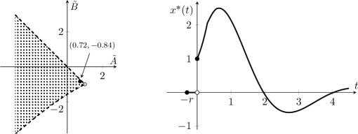
Figure 1: Left: Stability region of the linear retarded equation $\dot{y}(t)=\tilde{A}y(t)+\tilde{B}y(t-1)$. The point $(0.72,-0.84)$ corresponds to the parameter values $A=2.4$, $B=-2.8$, $r=0.3$ in the example from Burgers (1999). Right: The fundamental solution $t\mapsto x^{\ast}(t)$ of the equation $\dot{x}(t)=2.4x(t)-2.8x(t-0.3)$

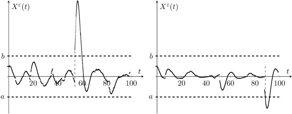
Figure 2: The most probable exit patterns of the perturbed delay equation $\dot{X}^{\varepsilon}(t)=2.4X^{\varepsilon}(t)-2.8X^{\varepsilon}(t-0.3)+\varepsilon\dot{Z}(t)$ from Burgers (1999). Left: The instant exit due to a large jump. Right: The exit due to a large jump and non-normal growth. In this case, the limiting exit location $X^{\varepsilon}(\tau^{\varepsilon})$ is supported by the end points $a$ and $b$.

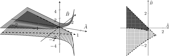
Figure 3: Left: The maximum $M$ and the infimum $m$ of the fundamental solution $y^{*}$ of the retarded delay equation $\dot{y}(t)=\tilde{A}y(t)+\tilde{B}y(t-1)$ for $(\tilde{A},\tilde{B})$ in the stability region. Right: The domain of parameters $(\tilde{A},\tilde{B})$ where $M=1$ and $m=0$. For these parameters, the asymptotics of the mean exit times (2.39) and (2.41) of the equation with and without delay coincide.

The most probable exit trajectories of the perturbed delay equation $\dot{X}^{\varepsilon}(t)=2.4X^{\varepsilon}(t)-2.8X^{\varepsilon}(t-0.3)+\varepsilon\dot{Z}(t)$ from Burgers (1999) are presented on Fig. 2. Taking into account the formulae (2.30) and (LABEL:e:epem) we find that the mean first exit time from an interval $[a,b]$ around zero satisfies

$$\mathbf{E}_{\varphi}\tau^{\varepsilon}\approx\frac{1}{2\varepsilon^{\alpha}}\Big{(}\frac{M^{\alpha}}{|a|^{\alpha}}\vee\frac{|m|^{\alpha}}{b^{\alpha}}+\frac{|m|^{\alpha}}{|a|^{\alpha}}\vee\frac{M^{\alpha}}{b^{\alpha}}\Big{)}^{-1}$$ (2.39)

where the values $M=M(A,B,r)$ and $m=m(A,B,r)$ depend on the values $A$, $B$, and $r$ in a complex nonlinear way, see Fig. 3. Denoting by $\tilde{M}=\tilde{M}(\tilde{A},\tilde{B})=M(Ar,Br,1)$ and $\tilde{m}=\tilde{m}(\tilde{A},\tilde{B})=m(Ar,Br,1)$ the extreme values of the fundamental solution $y^{*}$ we get that

$$\mathbf{E}_{\varphi}\tau^{\varepsilon}\approx\frac{1}{2\varepsilon^{\alpha}}\Big{(}\frac{\tilde{M}^{\alpha}}{|a|^{\alpha}}\vee\frac{|\tilde{m}|^{\alpha}}{b^{\alpha}}+\frac{|\tilde{m}|^{\alpha}}{|a|^{\alpha}}\vee\frac{\tilde{M}^{\alpha}}{b^{\alpha}}\Big{)}^{-1}.$$ (2.40)

The equation without delay, i.e. for $B=0$, is stable for $A<0$ with the fundamental solution $x^{*}(t)=\mathrm{e}^{At}$, so that $M=1$ and $m=0$, and mean exit time has the asymptotics

$$\mathbf{E}_{\varphi}\tau^{\varepsilon}\approx\frac{1}{2\varepsilon^{\alpha}}\Big{(}\frac{1}{|a|^{\alpha}}+\frac{1}{b^{\alpha}}\Big{)}^{-1},$$ (2.41)

see Godovanchuk (1982); Imkeller and Pavlyukevich (2006a, b). It is interesting to note that $M=1$ and $m=0$ holds for parameters $\tilde{A}=Ar$ and $\tilde{B}=Br$ from a larger domain. This domain can be determined numerically and is depicted on Fig. 3. For parameters in this domain, the asymptotics of the mean exit times (2.39) and (2.41) of the equation with and without delay coincide, and the asymptotic exit location has no atoms in $a$ and $b$. Hence, the first exit dynamics of the delay equation is effectively the same as for the equation without delay.

Eventually it is instructive to compare our results with the asymptotics of the exit time in the Gaussian case which has been studied for the first time by Zabczyk (1987).

Example 2.7 (Example 1, Zabczyk (1987)).

Consider a linear retarded equation driven by the Brownian additive noise

$$\dot{X}^{\varepsilon}(t) =AX^{\varepsilon}(t)+BX^{\varepsilon}(t-r)+\varepsilon\dot{W}(t),\quad t\geq 0,$$ (2.42)

$$X^{\varepsilon}(t) =\varphi(t),\ t\in[-r,0],$$

The stability region of this equation has been described in the previous example. With the help of the large deviations theory one obtains that for any $\varphi$ with no exit (see (2.21))

$$\varepsilon^{2}\ln\mathbf{E}_{\varphi}\tau^{\varepsilon}\sim\frac{(a\wedge b)^{2}}{rG(\tilde{A},\tilde{B})},$$ (2.43)

where the value $G$ is obtained in terms of the fundamental solution $y^{\ast}$ of $\dot{y}(t)=\tilde{A}y(t)+\tilde{B}y(t-1)$:

$$G(\tilde{A},\tilde{B})=2\int_{0}^{\infty}(y^{*}(t))^{2}\,\mathrm{d}t =\frac{2}{\pi}\int_{0}^{\infty}\frac{\mathrm{d}t}{(\tilde{A}+\tilde{B}\cos t)^{2}+(t+\tilde{B}\sin t)^{2}}$$ (2.44)

$$=\begin{cases}\displaystyle\frac{\tilde{B}q^{-1}\sin q-1}{\tilde{A}+\tilde{B}\cos q},\quad\tilde{B}+|\tilde{A}|<0,\ q=\sqrt{\tilde{B}^{2}-\tilde{A}^{2}},\\ \displaystyle\frac{1+|\tilde{A}|}{2|\tilde{A}|},\quad\tilde{B}=\tilde{A}<0,\\ \displaystyle\frac{\tilde{B}q^{-1}\sinh q-1}{\tilde{A}+\tilde{B}\cosh q},\quad\tilde{A}+|\tilde{B}|<0,\ q=\sqrt{\tilde{A}^{2}-\tilde{B}^{2}},\end{cases}$$

see (Shaikhet, 2011, Lemma 1.5). For the equation without delay, i.e. with $B=\tilde{B}=0$ one gets from (2.43) and (2.44) the well known exponentially large Kramers’ time

$$\mathbf{E}_{\varphi}\tau^{\varepsilon}\sim\mathrm{e}^{|A|\frac{(a\wedge b)^{2}}{\varepsilon^{2}}},\quad A<0.$$ (2.45)

3 Conclusion

In this article we solve the first exit time and location problem from an interval $[a,b]$, $a<0<b$, in a general class of stable linear delay differential equations for $\varepsilon$-small multiplicative, power law noise, such as $\alpha$-stable Lévy flights. In particular, we cover the linearization of gradient systems close to a stable state.

We recover, on the one hand, the asymptotic polynomial exit rate of the order $\varepsilon^{-\alpha}$ known in different Markovian settings which comes with an $\varepsilon$-independent prefactor. In the delay case this prefactor depends nonlinearly on the memory depth $r>0$ and can significantly reduce the expected exit times compared to the non-delay case reflecting a non-normal growth phenomena of the deterministic delay dynamics which changes the stochastic dynamics. This mirrors the situation for Brownian perturbations, where such an effect has been known since a long time as explained in Example 2.7. The case of retarded equations is explained in detail in Example 2.6.

Secondly, this non-normal growth becomes evident in the limiting exit location from the interval $[a,b]$ where in contrast to the non-delay case with jump exits we detect a point mass on the boundary. This mass stems from random trajectories which exit essentially due to deterministic motion.

The method of proof applied in the mathematical appendix consists of a series of elementary but new estimates valid for general Markov processes and well suited to be adapted to other settings.

4 Mathematical Appendix: Proof of the main Theorem 2.2

4.1 General estimates

This section reduces the first exit problem in three consecutive steps from a global problem to several smaller problems all of which are local in nature. We start by showing that the perturbed dynamics is dominated by the deterministic dynamics plus the error term of the perturbation. This is carried out for rather general perturbations by stochastic processes given as semimartingales, which include the stochastic integrals $\varepsilon\int_{0}^{t}F(X^{\varepsilon}_{s})(0-)\,\mathrm{d}Z(s)$ under consideration in (2.6). In the sequel we show that the solution driven only by bounded jumps, that is, before a first large jump happens remains close to the deterministic solution. Finally we establish upper and lower bounds for the distribution tails and the expectation of the exit times (including exit locations) for general Markov processes provided we have enough control over the short term behavior, which is left for Section 4.3 in order to conclude.

4.1.1 Estimates on the perturbed dynamics

For generalities of semimartingales we refer to the book by Protter (2004). In general, semimartingales are the class of stochastic Itô integral processes.

Lemma 4.1.

Let $S$ be a càdlàg semimartingale, $S(0)=0$, $\varphi\in D[-r,0]$ and let $X$ be a stochastic process satisfying

$$X(t,\varphi) =\varphi(0)+\int_{0}^{t}\Big{[}\int_{[-r,0]}X(s+u,\varphi)\,\mu(\mathrm{d}u)\Big{]}\,\mathrm{d}s+S(t),\qquad t\geq 0,$$ (4.1)

$$X(t,\varphi) =\varphi(t),\quad t\in[-r,0).$$

Then for each $\lambda\in(0,\Lambda)$ there is $C=C(\lambda,\mu,r)>0$ such that for $t\geq 0$

$$|X(t,\varphi)|\leq C\cdot\Big{(}\|\varphi\|_{r}\cdot\mathrm{e}^{-\lambda t}+\sup_{s\in[0,t]}|S(s)|\Big{)},$$ (4.2)

$$|X(t,\varphi)-\varphi(0)x^{*}(t)|\leq C\cdot\Big{(}\sup_{s\in[-r,0)}|\varphi(s)|\cdot\mathrm{e}^{-\lambda t}+\sup_{s\in[0,t]}|S(s)|\Big{)},$$ (4.3)

$$|X(t,\varphi)-x(t,\varphi)|\leq C\cdot\sup_{s\in[0,t]}|S(s)|.$$ (4.4)

Inequality (4.2) estimates the growth of the perturbed solution $X$ in terms of the size of the initial segment and the perturbation $S$, whereas (4.3) quantifies the memory effect in the initial segment and the noise. Inequality (4.4) controls the deviation caused by the noise alone.

Proof.

Let $\lambda\in(0,\Lambda)$ and the corresponding $K=K(\lambda)$ in estimate (2.12) be fixed.

1. By linearity we note that the the difference $Y(t;\varphi)=X(t;\varphi)-X(t;0)$ satisfies the homogeneous deterministic delay equation (2.1), that is, $Y(t;\varphi)=x(t;\varphi)$ for all $t\geq-r$, and hence the convolution formula (2.2) immediately implies

$$|Y(t)| \leq K|\varphi(0)|\cdot\mathrm{e}^{-\lambda t}+K\int_{[-r,0]}\Big{[}\int_{u}^{0}\Big{[}\mathrm{e}^{-\lambda(t-s+u)}\cdot|\varphi(s)|\,\mathrm{d}s\Big{]}\,|\mu(\mathrm{d}u)|$$ (4.5)

$$\leq K\cdot|\varphi(0)|\cdot\mathrm{e}^{-\lambda t}+K\cdot\frac{(e^{\lambda r}-1)}{\lambda}\cdot\|\varphi\|_{r}\cdot|\mu|[-r,0]\cdot\mathrm{e}^{-\lambda t}$$

$$\leq C_{1}(\lambda,r,\mu)\|\varphi\|_{r}\cdot\mathrm{e}^{-\lambda t},$$

where $|\mu|$ stands for the standard total variation measure of the finite signed measure $\mu$.

Now we apply the stability of the unperturbed system comparing $X(\cdot;0)$ to the following Ornstein–Uhlenbeck type process $U$ given by

$$U(t)=\begin{cases}-\displaystyle\lambda\int_{0}^{t}U(s)\,\mathrm{d}s+S(t)&\mbox{ for }t\geq 0,\\ 0&\mbox{ for }t\in[-r,0).\end{cases}$$ (4.6)

The process $U$ has the explicit solution

$$U(t)=\int_{0}^{t}\mathrm{e}^{-\lambda(t-s)}\,\mathrm{d}S(s),\quad t\geq 0.$$ (4.7)

Integration by parts then yields $U(t)=S(t)-\lambda\mathrm{e}^{-\lambda t}\int_{0}^{t}S(s)\mathrm{e}^{\lambda s}\,\mathrm{d}s$, such that

$$|U(t)| \leq 2\sup_{s\in[0,t]}|S(s)|.$$ (4.8)

We fix the notation $V(t):=X(t;0)-U(t)$, $t\geq-r$, and note that $X(\cdot;0)=V+U$. It remains to estimate $V$. Collecting the absolutely continuous parts as

$$A(t):=\int_{0}^{t}\Big{[}\int_{[-r,0]}U(s+u)\,\mu(\mathrm{d}u)\Big{]}\,\mathrm{d}s-\lambda\int_{0}^{t}U(s)\,\mathrm{d}s$$ (4.9)

we obtain the following equation for $V$

$$V(t) =X(t;0)-U(t)$$ (4.10)

$$=\int_{0}^{t}\int_{[-r,0]}\Big{(}X(s+u;0)-U(s+u)\Big{)}\,\mu(\mathrm{d}u)\,\mathrm{d}s+\int_{0}^{t}\int_{[-r,0]}U(s+u)\,\mu(\mathrm{d}u)\,\mathrm{d}s-\lambda\int_{0}^{t}U(s)\,\mathrm{d}s$$

$$=\int_{0}^{t}\int_{[-r,0]}V(s+u)\,\mu(\mathrm{d}u)\,\mathrm{d}s+A(t),$$

the solution of which has the explicit convolution representation

$$V(t)=\int_{0}^{t}x^{*}(t-s)A^{\prime}(s)\,\mathrm{d}s,$$ (4.11)

where

$$A^{\prime}(t)=\int_{[-r,0]}U(t+u)\,\mu(\mathrm{d}u)-\lambda U(t).$$ (4.12)

Equation (4.11) and inequality (2.12) then yield the estimate

$$|V(t)|\leq K\int_{0}^{t}\mathrm{e}^{-\lambda(t-s)}|A^{\prime}(s)|\,\mathrm{d}s,\quad t\geq 0.$$ (4.13)

Furthermore, (4.12) implies for some $C_{2}=C_{2}(\lambda,\mu,r)>0$

$$|A^{\prime}(t)| \leq|\mu|[-r,0]\cdot\sup_{u\in[-r,0]}|U(t+u)|+\lambda|U(t)|$$ (4.14)

$$\leq\Big{(}|\mu|[-r,0]+\lambda\Big{)}\sup_{u\in[-r,0]}|U(t+u)|$$

$$\leq C_{2}\cdot\sup_{s\in[0,t]}|U(s)|.$$

Combining the two preceding inequalities results in a constant $C_{3}=C_{3}(\lambda,K,\mu,r)>0$ such that

$$|V(t)| =K\cdot C_{2}\cdot\sup_{s\in[0,t]}|U(s)|\cdot\int_{0}^{t}\mathrm{e}^{-\lambda(t-s)}\,\mathrm{d}s\leq\frac{K\cdot C_{2}}{\lambda}\cdot\sup_{s\in[0,t]}|U(s)|=C_{3}\cdot\sup_{s\in[0,t]}|U(s)|$$ (4.15)

and (4.2) follows as a combination of (4.5), (4.8) and (4.15).

2. We denote the perturbed fundamental solution with initial segment $\varphi(0)\mathbb{I}_{\{0\}}$ by $\tilde{X}$. It satisfies

$$\tilde{X}(t)=\varphi(0)+\int_{0}^{t}\int\tilde{X}(s+u)\,\mu(\mathrm{d}u)\,\mathrm{d}s+S(t),$$ (4.16)

$$\tilde{X}(t)=0,\quad t\in[-r,0).$$

Then

$$X(t;\varphi)-\varphi(0)x^{*}(t)=X(t;\varphi)-\tilde{X}(t)+\tilde{X}(t)-\varphi(0)x^{*}(t)$$ (4.17)

and $\tilde{Y}(t):=X(t,\varphi)-\tilde{X}(t)$ is the solution of

$$\tilde{Y}(t)=\int_{0}^{t}\Big{[}\int_{[-r,0]}\tilde{Y}(s+u)\,\mu(\mathrm{d}u)\Big{]}\,\mathrm{d}s,$$ (4.18)

$$\tilde{Y}(t)=\varphi(t),\quad t\in[-r,0).$$

Hence arguing as for the term $A$ in part 1. we get

$$|\tilde{Y}(t)|\leq C_{1}\cdot\sup_{s\in[-r,0)}|\varphi(s)|\cdot\mathrm{e}^{-\lambda t}$$ (4.19)

with the same constant $C_{1}$ as in (4.5). Analogously to the identification of $Y$ in part 1. we observe

$$\tilde{X}(t)-\varphi(0)x^{*}(t)=X(t;0)=V(t)+U(t),$$ (4.20)

where the processes $V$ and $U$ are already estimated in (4.8) and (4.15) of part 1. Inequality (4.3) then follows by

$$|X(t,\varphi)-\varphi(0)x^{*}(t)|\leq|\tilde{Y}(t)|+|V(t)|+|U(t)|\leq C_{1}\sup_{[-r,0)}|\varphi(s)|\mathrm{e}^{-\lambda t}+2(C_{3}+1)\sup_{s\in[0,t]}|S(s)|.$$ (4.21)

3. Since $X(t;\varphi)-x(t;\varphi)=X(t;0)=V(t)+U(t)$, estimate (4.4) follows immediately by the previous results. ∎

4.1.2 Estimates on the stochastic perturbation

Let us rewrite the underlying Lévy process $Z$ as a sum of a compound Poisson process

$$\eta^{\rho}(t) =\sum_{s\leq t}\Delta Z(s)\mathbb{I}(|\Delta Z(s)|>\rho),\qquad t\geq 0,$$ (4.22)

whose jumps are larger than some threshold $\rho>1$ in absolute value, and an independent Lévy process $\xi^{\rho}=Z-\eta^{\rho}$ with bounded jumps. This is always possible and can be easily seen by comparison of the Lévy–Khintchine formula (2.3) for $Z$ with those for $\eta^{\rho}$ and $\xi^{\rho}$

$$\ln\mathbf{E}\mathrm{e}^{\mathrm{i}u\eta^{\rho}(t)}=t\int_{|z|>\rho}(\mathrm{e}^{\mathrm{i}uz}-1)\,\nu(\mathrm{d}z),$$ (4.23)

$$\ln\mathbf{E}\mathrm{e}^{\mathrm{i}u\xi^{\rho}(t)}=-\frac{\sigma^{2}}{2}u^{2}t+\mathrm{i}\,d_{\rho}ut+t\int_{|z|\leq\rho}(\mathrm{e}^{\mathrm{i}uz}-1-\mathrm{i}uz)\,\nu(\mathrm{d}z),$$

where the new drift $d_{\rho}=d+\int_{1<|z|\leq\rho}z\,\nu(\mathrm{d}z)$. We denote the jump times and sizes of $\eta^{\rho}$ by $\{\tau_{k}\}_{k\geq 1}$, and $\{J_{k}\}_{k\geq 1}$ respectively and recall that they are independent. Moreover, the interjump times $\tau_{1},\tau_{2}-\tau_{1}$,…, are iid exponentially distributed random variables with the parameter

$$\beta_{\rho}=\int_{|z|>\rho}\nu(\mathrm{d}z),$$ (4.24)

and the jump sizes $\{J_{k}\}_{k\geq 1}$ are also iid with the probability law

$$\mathbf{P}(J_{k}\in A)=\frac{1}{\beta_{\rho}}\int_{|z|>\rho}\mathbb{I}_{A}(z)\,\nu(\mathrm{d}z),\quad A\in\mathscr{B}(\mathbb{R}).$$ (4.25)

Let $X^{\varepsilon}=X^{\varepsilon}(\cdot;\varphi)$ be the solution to the delay SDDE (2.6), and consider the stochastic integral process

$$S^{\varepsilon,\rho}(t)=\varepsilon\int_{0}^{t}F(X^{\varepsilon}_{s})(0-)\,\mathrm{d}\xi^{\rho}(s).$$ (4.26)

Remark 4.2.

In this article we are interested in the first exit time of $X^{\varepsilon}(t)$ from the interval $[a,b]$, which coincides by definition by the first exit time of $X^{\varepsilon}_{t}$ in segment space from the segment interval $\ldbrack a,b\rdbrack_{r}$. By the Lipschitz continuity (2.4) we have

$$\sup_{\varphi\in\ldbrack a,b\rdbrack_{r}}\|F(\varphi)\|_{r}\leq L(\|F(0)\|_{r}+\sup_{\varphi\in\ldbrack a,b\rdbrack_{r}}\|\varphi\|_{r}).$$

That is, before the first exit $t\leq\tau$ the coefficient of (4.26) is bounded by

$$\|F(X^{\varepsilon})(t-)\|_{r}\leq L(\|F(0)\|_{r}+\max\{|a|,b\})<\infty.$$

Therefore it is without a loss of generality if we assume that $F$ is uniformly bounded, that is, $\sup_{\varphi\in D[-r,0]}\|F(\varphi)\|_{r}\leq C_{F}<\infty$ for some global constant $C_{F}>0$.

Lemma 4.3.

Let $F$ be uniformly bounded by a constant $C_{F}>0$. Then for any $\rho>1$, $T>0$, $\delta>0$ and any $p>1$ there is a constant $C_{S}>0$ such that for any $0\leq s\leq t\leq T$ and $\varepsilon>0$ sufficiently small we have

$$\mathbf{P}\Big{(}\sup_{u\in[0,t-s]}|S^{\varepsilon,\rho}(s+u)-S^{\varepsilon,\rho}(s)|>\delta\Big{)}\leq C_{S}\varepsilon^{p}.$$ (4.27)

Proof.

Note that $\tilde{\xi}^{\rho}(t)=\xi^{\rho}(t)-d_{\rho}t$, $t\geq 0$, is a martingale with bounded jumps, as well as for fixed $s\geq 0$ the stochastic integral process $\tilde{S}^{\varepsilon,\rho}(s+u)-\tilde{S}^{\varepsilon,\rho}(s)=\varepsilon\int_{s}^{s+u}F(X^{\varepsilon}_{v})(0-)\,\mathrm{d}\tilde{\xi}^{\rho}(v)$, $u\geq 0$. Then the triangle inequality, the Markov inequality, and the classical Burkholder-Davis-Gundy inequality for $p>1$ (see for instance Protter (2004), Theorem 4.8) yield a constant $C_{p}>0$ such that for $\varepsilon>0$ being sufficiently small it follows

$$\mathbf{P}\Big{(}\sup_{u\in[0,t-s]} |S^{\varepsilon,\rho}(s+u)-S^{\varepsilon,\rho}(s)|>\delta\Big{)}$$ (4.28)

$$\leq\mathbf{P}\Big{(}\varepsilon\cdot C_{F}\cdot|d_{\rho}|\cdot T>\frac{\delta}{2}\Big{)}+\mathbf{P}\Big{(}\sup_{u\in[0,t-s]}\Big{|}\varepsilon\int_{s}^{s+u}F(X^{\varepsilon}_{v})(0-)\,\mathrm{d}\tilde{\xi}^{\rho}(v)\Big{|}>\frac{\delta}{2}\Big{)}$$

$$\leq 0+\varepsilon^{p}\cdot\frac{2^{p}}{\delta^{p}}\leavevmode\nobreak\ \mathbf{E}\sup_{u\in[s,t-s]}\Big{|}\int_{s}^{s+u}F(X^{\varepsilon}_{v})(0-)\,\mathrm{d}\tilde{\xi}^{\rho}(v)\Big{|}^{p}$$

$$\leq\varepsilon^{p}\cdot\frac{2^{p}C_{p}}{\delta^{p}}T^{p/2}\cdot C_{F}^{p}\cdot\Big{(}\sigma^{2}+\int_{|z|\leq\rho}z^{2}\,\nu(\mathrm{d}z)\Big{)}^{p/2}=C_{S}\cdot\varepsilon^{p}.$$

∎

4.2 General segment Markov estimates

Let $X$ be a càdlàg segment Markov process as given in (2.9) and denote for $a<0<b$ the first exit time of $X$ from $[a,b]$ by

$$\tau=\tau(\varphi)=\inf\{t\geq 0\colon X(t)\notin[a,b]\}.$$ (4.29)

Lemma 4.4.

If for some $T\geq r>0$, $m_{1}$, $m_{2}>0$ satisfying $m_{1}T\leq m_{2}T<1$ and $p_{1}(B)$, $p_{2}(B)>0$ we have the short term estimates

$$\inf_{\varphi\in\ldbrack a,b\rdbrack_{r}}\mathbf{P}_{\varphi}(\tau\leq T)\geq m_{1}T,$$ (4.30)

$$\inf_{\varphi\in\ldbrack a,b\rdbrack_{r}}\mathbf{P}_{\varphi}(\tau\leq T,X(\tau)\in B)\geq m_{1}T\cdot p_{1}(B),$$ (4.31)

$$\sup_{\varphi\in\ldbrack a,b\rdbrack_{r}}\mathbf{P}_{\varphi}(\tau\leq T,X(\tau)\in B)\leq m_{2}T\cdot p_{2}(B),$$ (4.32)

then for each $u\geq 0$ we have

$$\sup_{\varphi\in\ldbrack a,b\rdbrack_{r}}\mathbf{P}_{\varphi}(\tau>u)\leq\frac{\mathrm{e}^{-um_{1}}}{1-m_{1}T},$$ (4.34)

$$\sup_{\varphi\in\ldbrack a,b\rdbrack_{r}}\mathbf{P}_{\varphi}(\tau>u,X(\tau)\in B)\leq\frac{\mathrm{e}^{-um_{1}}}{(1-m_{1}T)^{2}}\cdot\Big{(}\frac{m_{2}}{m_{1}}p_{2}(B)-m_{1}Tp_{1}(B)\Big{)},$$ (4.35)

$$\sup_{\varphi\in\ldbrack a,b\rdbrack_{r}}\mathbf{P}_{\varphi}(X(\tau)\in B)\leq\frac{m_{2}}{m_{1}}\cdot p_{2}(B)$$ (4.36)

and

$$\sup_{\varphi\in\ldbrack a,b\rdbrack_{r}}\mathbf{E}_{\varphi}\tau \leq\frac{1}{m_{1}}.$$ (4.37)

Proof.

We first show (4.35). For each $u>0$ denote $k=\lfloor\frac{u}{T}\rfloor$. Then $kT\leq u$ and

$$\mathbf{P}_{\varphi}(\tau>u,X(\tau)\in B)\leq\mathbf{P}_{\varphi}(\tau>kT,X(\tau)\in B).$$ (4.38)

The segment Markov property and (4.30) yield for any initial condition $\varphi\in\ldbrack a,b\rdbrack_{r}$

$$\mathbf{P}_{\varphi}(\tau>kT,X(\tau)\in B) =\mathbf{E}_{\varphi}\Big{[}\mathbb{I}(\tau>kT,X(\tau)\in B)\cdot\mathbb{I}(\tau>(k-1)T)\Big{]}$$ (4.39)

$$=\mathbf{E}_{\varphi}\mathbf{E}\Big{[}\mathbb{I}(\tau>kT,X(\tau)\in B)\cdot\mathbb{I}(\tau>(k-1)T)\Big{|}\mathscr{F}_{(k-1)T}\Big{]}$$

$$=\mathbf{E}_{\varphi}\Big{[}\mathbb{I}(\tau>(k-1)T)\cdot\mathbf{E}\Big{[}\mathbb{I}(\tau>kT,X(\tau)\in B)\cdot\Big{|}\mathscr{F}_{(k-1)T}\Big{]}\Big{]}$$

$$=\mathbf{E}_{\varphi}\Big{[}\mathbb{I}(\tau>(k-1)T)\cdot\mathbf{E}_{X_{(k-1)T}}\Big{[}\mathbb{I}(\tau>T,X(\tau)\in B)\Big{]}\Big{]}$$

$$\leq\mathbf{P}_{\varphi}\Big{(}\tau>(k-1)T)\Big{)}\cdot\sup_{\psi\in\ldbrack a,b\rdbrack_{r}}\mathbf{P}_{\psi}(\tau>T,X(\tau)\in B)$$

$$\leq\Big{[}1-\inf_{\varphi\in\ldbrack a,b\rdbrack_{r}}\mathbf{P}_{\varphi}(\tau\leq T)\Big{]}^{k-1}\cdot\sup_{\psi\in\ldbrack a,b\rdbrack_{r}}\mathbf{P}_{\psi}(\tau>T,X(\tau)\in B)$$

$$\leq(1-m_{1}T)^{k-1}\cdot\sup_{\psi\in\ldbrack a,b\rdbrack_{r}}\mathbf{P}_{\psi}(\tau>T,X(\tau)\in B).$$

While the first term satisfies

$$(1-m_{1}T)^{k-1}=\frac{(1-\frac{m_{1}kT}{k})^{k}}{1-m_{1}T}\leq\frac{(1-\frac{m_{1}u}{k})^{k}}{1-m_{1}T}\leq\frac{\mathrm{e}^{-m_{1}u}}{1-m_{1}T}.$$ (4.40)

The last inequality is given by $\mathrm{e}^{-m_{1}u}-(1-m_{1}u/k)^{k}\geq 0$ for all $m_{1}u\leq k$. The latter condition is satisfied since $m_{1}kT\leq m_{1}u\leq k$, which is a consequence of $m_{1}T<1$ in the statement. We rewrite the last term on the right side of (4.39) as

$$\mathbf{P}_{\varphi}(\tau>T,X(\tau)\in B)=\mathbf{P}_{\varphi}(X(\tau)\in B)-\mathbf{P}_{\varphi}(\tau\leq T,X(\tau)\in B).$$ (4.41)

While the second term is estimated by (4.31) we calculate the first summand, which is (4.36), with the segment Markov property and (4.30)

$$\mathbf{P}_{\varphi}(X(\tau)\in B) =\sum_{k=1}^{\infty}\mathbf{P}_{\varphi}(X(\tau)\in B,(k-1)T<\tau\leq kT)$$ (4.42)

$$=\sum_{k=1}^{\infty}\mathbf{E}_{\varphi}\mathbf{E}\Big{[}\mathbb{I}((k-1)T<\tau,X(\tau)\in B,\tau\leq kT)\Big{|}\mathscr{F}_{(k-1)T}\Big{]}\Big{]}$$

$$=\sum_{k=1}^{\infty}\mathbf{E}_{\varphi}\mathbf{E}\Big{[}\mathbb{I}((k-1)T<\tau,X(\tau)\in B,\tau^{\varepsilon}\leq kT)\Big{|}\mathscr{F}_{(k-1)T}\Big{]}\Big{]}$$

$$=\sum_{k=1}^{\infty}\mathbf{E}_{\varphi}\mathbb{I}((k-1)T<\tau)\cdot\mathbf{P}_{X_{(k-1)T}}(X(\tau)\in B,\tau^{\varepsilon}\leq T)\Big{]}$$

$$\leq\sup_{\psi\in\ldbrack a,b\rdbrack_{r}}\mathbf{P}_{\psi}(X(\tau)\in B,\tau\leq T)\cdot\sum_{k=1}^{\infty}\mathbf{P}_{\varphi}((k-1)T<\tau)$$

$$\leq m_{2}\cdot T\cdot p_{2}(B)\cdot\sum_{k=1}^{\infty}\Big{(}1-m_{1}T\Big{)}^{k-1}$$

$$=\frac{m_{2}}{m_{1}}\cdot p_{2}(B).$$

The estimates (4.41) and (4.42) yield

$$\mathbf{P}_{\varphi}(\tau>T,X(\tau)\in B)\leq m_{2}T\cdot p_{2}(B)\cdot\frac{1}{m_{1}T}-m_{1}Tp_{1}(B)$$ (4.43)

and (4.38)-(4.40) with (4.43) imply (4.35). Setting $B=\mathbb{R}$ estimate (4.34) follows directly from (4.38)-(4.40). Eventually

$$\mathbf{E}_{\varphi}\tau \leq T\sum_{k=1}^{\infty}k\cdot\mathbf{P}_{\varphi}((k-1)T<\tau\leq kT)=T\sum_{k=0}^{\infty}k\cdot\mathbf{P}_{\varphi}(\tau>Tk)\leq T\sum_{k=0}^{\infty}(1-m_{1}T)^{k}=\frac{1}{m_{1}}.$$ (4.44)

∎

Lemma 4.5.

Let $B$ be a Borel set. If for some $T\geq r>0$, $m_{1},m_{2}>0$ satisfying $m_{1}T\leq m_{2}T<1$, $p_{1}(B),p_{2}(B)\leq 1$ and $\delta\in(0,|a|\wedge b)$ we have the short term estimates

$$\sup_{\|\varphi\|_{r}\leq\delta}\mathbf{P}_{\varphi}(\tau\leq T,X(\tau)\in B)\leq m_{1}T\cdot p_{1}(B),$$ (4.45)

$$\inf_{\|\varphi\|_{r}\leq\delta}\mathbf{P}_{\varphi}(\tau\leq T,X(\tau)\in B)\geq m_{2}T\cdot p_{2}(B),$$ (4.46)

$$\inf_{\|\varphi\|_{r}\leq\delta}\mathbf{P}_{\varphi}(\tau>T,\|X_{T}\|_{r}\leq\delta)\geq 1-m_{1}T,$$ (4.47)

then for each $u\geq 0$ we get

$$\inf_{\|\varphi\|_{r}\leq\delta}\mathbf{P}_{\varphi}(\tau>u,X(\tau)\in B)\geq(1-m_{1}T)\mathrm{e}^{-\frac{u}{T}\ln(1-m_{1}T)}\cdot\Big{(}\frac{m_{2}}{m_{1}}\cdot p_{2}(B)-m_{1}Tp_{1}(B)\Big{)},$$ (4.48)

$$\inf_{\|\varphi\|_{r}\leq\delta}\mathbf{P}_{\varphi}(X(\tau)\in B)\geq\frac{m_{2}}{m_{1}}p_{2}(B).$$ (4.49)

$$\inf_{\|\varphi\|_{r}\leq\delta}\mathbf{E}_{\varphi}\tau\geq\frac{1-m_{1}T}{m_{1}}.$$ (4.50)

Proof.

For each $u>0$ denote $k=\lceil\frac{u}{T}\rceil$. In particular $(k-1)T<u\leq kT$. Then the segment Markov property and (4.47) yield for any initial condition $\|\varphi\|_{r}\leq\delta$

$$\mathbf{P}_{\varphi}(\tau>u)\geq\mathbf{P}_{\varphi}(\tau>kT) \geq\mathbf{E}_{\varphi}\Big{[}\mathbb{I}(\tau>kT)\cdot\mathbb{I}(\tau>(k-1)T)\cdot\mathbb{I}(\|X_{(k-1)T}\|_{r}\leq\delta)\Big{]}$$ (4.51)

$$=\mathbf{E}_{\varphi}\mathbf{E}\Big{[}\mathbb{I}(\tau>kT)\cdot\mathbb{I}(\tau>(k-1)T)\cdot\mathbb{I}(\|X_{(k-1)T}\|_{r}\leq\delta)\Big{|}\mathscr{F}_{(k-1)T}\Big{]}$$

$$=\mathbf{E}_{\varphi}\Big{[}\mathbb{I}(\tau>(k-1)T)\cdot\mathbb{I}(\|X_{(k-1)T}\|_{r}\leq\delta)\mathbf{E}\Big{[}\mathbb{I}(\tau>kT)\Big{|}\mathscr{F}_{(k-1)T}\Big{]}\Big{]}$$

$$=\mathbf{E}_{\varphi}\mathbb{I}(\tau>(k-1)T)\cdot\mathbb{I}(\|X_{(k-1)T}\|_{r}\leq\delta)\mathbf{E}_{X_{(k-1)T}}\Big{[}\mathbb{I}(\tau>kT)\Big{]}$$

$$\geq\mathbf{P}_{\varphi}\Big{(}\tau>(k-1)T,\|X_{(k-1)T}\|_{r}\leq\delta\Big{)}\cdot\inf_{\|\psi\|_{r}\leq\delta}\mathbf{P}_{\psi}\Big{(}\tau>T\Big{)}$$

$$\geq\Big{[}\inf_{\|\psi\|_{r}\leq\delta}\mathbf{P}_{\psi}\Big{(}\tau>T,\|X_{T}\|_{r}\leq\delta\Big{)}\Big{]}^{k-1}\cdot\inf_{\|\psi\|_{r}\leq\delta}\mathbf{P}_{\psi}\Big{(}\tau>T\Big{)}$$

$$\geq(1-m_{1}T)^{k}$$

and (4.50) follows by

$$\mathbf{E}_{\varphi}\tau \geq T\sum_{k=1}^{\infty}(k-1)\cdot\mathbf{P}_{\varphi}((k-1)T<\tau\leq kT)$$ (4.52)

$$=T\sum_{k=1}^{\infty}\mathbf{P}_{\varphi}(\tau>Tk)\geq T\sum_{k=1}^{\infty}(1-m_{1}T)^{k}=\frac{1-m_{1}T}{m_{1}}.$$

Furthermore, inequality (4.49) is a result from

$$\mathbf{P}_{\varphi}(X(\tau)\in B) =\sum_{k=1}^{\infty}\mathbf{P}_{\varphi}(X(\tau)\in B,(k-1)T<\tau\leq kT)$$ (4.53)

$$\geq\sum_{k=1}^{\infty}\mathbf{E}_{\varphi}\Big{[}\mathbb{I}(\tau>(k-1)T)\cdot\mathbb{I}(\|X_{(k-1)T}\|_{r}\leq\delta)\mathbf{E}\Big{[}\mathbb{I}(X(\tau)\in B,\tau\leq kT)\Big{|}\mathscr{F}_{(k-1)T}\Big{]}\Big{]}$$

$$\geq\inf_{\|\psi\|_{r}\leq\delta}\mathbf{P}_{\psi}\Big{(}X(\tau)\in B,\tau\leq T\Big{)}\cdot\sum_{k=1}^{\infty}\mathbf{P}_{\varphi}\Big{(}\tau>(k-1)T,\|X_{(k-1)T}\|_{r}\leq\delta\Big{)}$$

$$\geq m_{2}T\cdot p_{2}(B)\cdot\sum_{k=1}^{\infty}(1-m_{1}T)^{k-1}$$

$$=\frac{m_{2}}{m_{1}}\cdot p_{2}(B).$$

Finally, repeating the chain of inequalities (4.51) with the additional event $\{X(\tau)\in B\}$, we get

$$\mathbf{P}_{\varphi}(\tau>u,\leavevmode\nobreak X(\tau)\in B)\geq\mathbf{P}_{\varphi}(\tau>kT,X(\tau)\in B)$$ (4.54)

$$\geq\mathbf{E}_{\varphi}\Big{[}\mathbb{I}(\tau>kT,X(\tau)\in B)\cdot\mathbb{I}(\tau>(k-1)T)\cdot\mathbb{I}(\|X_{(k-1)T}\|_{r}\leq\delta)\Big{]}$$

$$=\mathbf{E}_{\varphi}\mathbf{E}\Big{[}\mathbb{I}(\tau>kT,X(\tau)\in B)\cdot\mathbb{I}(\tau>(k-1)T)\cdot\mathbb{I}(\|X_{(k-1)T}\|_{r}\leq\delta)\Big{|}\mathscr{F}_{(k-1)T}\Big{]}$$

$$\geq\mathbf{P}_{\varphi}\Big{(}\tau>(k-1)T,\|X_{(k-1)T}\|_{r}\leq\delta\Big{)}\cdot\inf_{\|\psi\|_{r}\leq\delta}\mathbf{P}_{\psi}\Big{(}\tau>T,X(\tau)\in B\Big{)}$$

$$\geq\Big{[}\inf_{\|\psi\|_{r}\leq\delta}\mathbf{P}_{\psi}\Big{(}\tau>T,\|X_{T}\|_{r}\leq\delta\Big{)}\Big{]}^{k-1}\cdot\inf_{\|\psi\|_{r}\leq\delta}\mathbf{P}_{\psi}\Big{(}\tau>T,X(\tau)\in B\Big{)}$$

$$\geq(1-m_{1}T)^{k}\cdot\Big{(}\frac{m_{2}}{m_{1}}\cdot p_{2}(B)-m_{1}T\cdot p_{1}(B)\Big{)},$$

and (4.48) follows directly. ∎

4.3 Proof of the main estimates

The main result will follow directly from the following six inequalities.

Lemma 4.6.

For any $\varkappa>0$ there is $T>0$ and $\varepsilon_{0}>0$ such that for all $\varepsilon\in(0,\varepsilon_{0}]$

$$\inf_{\varphi\in\ldbrack a,b\rdbrack_{r}}\mathbf{P}_{\varphi}(\tau^{\varepsilon}\leq T)\geq\lambda_{\varepsilon}\bar{\nu}(E)T(1-\varkappa).$$ (4.55)

Lemma 4.7.

For any $\varkappa>0$ there are $\delta>0$, $T>0$, and $\varepsilon_{0}>0$ such that for all $\varepsilon\in(0,\varepsilon_{0}]$

$$\inf_{\|\varphi\|_{r}\leq\delta}\mathbf{P}_{\varphi}(\tau^{\varepsilon}>T,\|X_{T}^{\varepsilon}\|_{r}\leq\delta)\geq 1-\lambda_{\varepsilon}\bar{\nu}(E)T(1+\varkappa).$$ (4.56)

Lemma 4.8.

For any $\varkappa>0$ and $v>b$ there is $T>0$ and $\varepsilon_{0}>0$ such that for all $\varepsilon\in(0,\varepsilon_{0}]$

$$\inf_{\varphi\in\ldbrack a,b\rdbrack_{r}}\mathbf{P}_{\varphi}(\tau^{\varepsilon}\leq T,X^{\varepsilon}(\tau^{\varepsilon})>v)\geq\lambda_{\varepsilon}T\cdot\bar{\nu}(E_{b}^{j}(v))(1-\varkappa).$$ (4.57)

Lemma 4.9.

For any $\varkappa>0$ and $v>b$ there is $T>0$ and $\varepsilon_{0}>0$ such that for all $\varepsilon\in(0,\varepsilon_{0}]$

$$\sup_{\varphi\in\ldbrack a,b\rdbrack_{r}}\mathbf{P}_{\varphi}(\tau^{\varepsilon}\leq T,X^{\varepsilon}(\tau^{\varepsilon})>v)\leq\lambda_{\varepsilon}T\cdot\bar{\nu}(E_{b}^{j}(v))(1+\varkappa).$$ (4.58)

Analogously to Lemmas 4.8 and 4.8 one proves the estimate for the exit into the set $(-\infty,a)$.

Lemma 4.10.

For any $\varkappa>0$ and $v<a$ there is $T>0$ and $\varepsilon_{0}>0$ such that for all $\varepsilon\in(0,\varepsilon_{0}]$

$$\inf_{\varphi\in\ldbrack a,b\rdbrack_{r}}\mathbf{P}_{\varphi}(\tau^{\varepsilon}\leq T,X^{\varepsilon}(\tau^{\varepsilon})<v)\geq\lambda_{\varepsilon}T\cdot\bar{\nu}(E_{a}^{j}(v))(1-\varkappa),$$ (4.59)

$$\sup_{\varphi\in\ldbrack a,b\rdbrack_{r}}\mathbf{P}_{\varphi}(\tau^{\varepsilon}\leq T,X^{\varepsilon}(\tau^{\varepsilon})<v)\leq\lambda_{\varepsilon}T\cdot\bar{\nu}(E_{a}^{j}(v))(1+\varkappa).$$ (4.60)

Before passing to the proof of the Lemmas we make several preparatory comments. Let $\varkappa>0$ be an arbitrary small number.

1. For $\gamma>-\min\{|a|,b\}$ denote

$$E(\gamma)=\{z\colon\exists\,t\geq 0\text{ such that }z\cdot F_{0}\cdot x^{*}(t)\notin[a-\gamma,b+\gamma]\}=[e_{-}(\gamma),e_{+}(\gamma)]^{c},\quad E(0)=E.$$ (4.61)

Assume that $\bar{\nu}(E)>0$. Due to the continuity of the fundamental solution,

$$\lim_{\gamma\to 0}e_{\pm}(\gamma)=e_{\pm}$$ (4.62)

and for any $\varkappa>0$ with the help of (2.14) we get

$$\frac{\nu(E(\gamma)/\varepsilon)}{\lambda_{\varepsilon}}=\frac{\nu(E(\gamma)/\varepsilon)}{\lambda_{\varepsilon}\bar{\nu}(E(\gamma))}\cdot\frac{\bar{\nu}(E(\gamma))}{\bar{\nu}(E)}\geq 1-\frac{\varkappa}{20}$$ (4.63)

for $\gamma$ and $\varepsilon$ sufficiently small.

2. Let $\lambda\in(0,\Lambda)$ and $K=K(\lambda)$ according to (2.12) be fixed. For any $\delta>0$ we can choose $R>r$ such that

$$\max\{|a|,b\}\cdot K\cdot\mathrm{e}^{-\lambda(R-r)}<\delta.$$ (4.64)

In particular, for any $\varphi\in\ldbrack a,b\rdbrack_{r}$ and $t\geq R$ we have.

$$|x(t,\varphi)|<\delta.$$ (4.65)

Note that $R$ also bounds the time horizon of a non-normal growth exit so that a deterministic exit can occur only before the time instant $R$.

3. For $\delta$ and $R$ chosen, we can fix $T>0$ such that

$$\frac{2R}{T}\leq\frac{\varkappa}{20}.$$ (4.66)

4. Finally, for $\delta>0$ and $0\leq s\leq t\leq T$ denote

$$\mathcal{E}_{s,t}=\mathcal{E}_{s,t}(\delta)=\Big{\{}\sup_{u\in[0,t-s]}|S^{\varepsilon,\rho}(s+u)-S^{\varepsilon,\rho}(s)|\leq\delta\Big{\}}.$$ (4.67)

With the help of Lemma 4.3 with $p>\alpha$ we get $\mathbf{P}(\mathcal{E}_{s,t}(\delta))=o(\lambda_{\varepsilon})$, and in particular

$$\mathbf{P}(\mathcal{E}_{s,t}(\delta))>1-\frac{\varkappa}{20}T\lambda_{\varepsilon}\bar{\nu}(E)$$ (4.68)

for $\varepsilon$ small enough.

4.3.1 Proof of Lemma 4.6

We show that with high probability the exit from $[a,b]$ is to occur imminently after the first large jump.

For $\delta=\delta(\varkappa,\gamma)>0$, $T=T(\delta)$ and $R=R(\delta)$ to be chosen later and for any $\varphi\in\ldbrack a,b\rdbrack_{r}$ we exclude the following error events which eventually turn out to have small probability and estimate

$$\mathbf{P}_{\varphi}(\tau^{\varepsilon}\leq T) \geq\mathbf{P}_{\varphi}(\tau^{\varepsilon}\leq T,\varepsilon J_{1}\in E(\gamma),R\leq\tau_{1}\leq T-R,\tau_{2}>T,\mathcal{E}_{0,\tau_{1}}(\delta),\mathcal{E}_{\tau_{1},T}(\delta)).$$ (4.69)

Now we show that with a proper choice of the parameters, the set of conditions $\{\varepsilon J_{1}\in E(\gamma)\}\cap\{R\leq\tau_{1}\leq T-R\}\cap\{\tau_{2}>T\}\cap\mathcal{E}_{0,\tau_{1}}\cap\mathcal{E}_{\tau_{1},T}$ will imply that the exit occurs before the time $T$, $\tau^{\varepsilon}\leq T$.

Indeed, at the time instant $\tau_{1}$ we have

$$X^{\varepsilon}(\tau_{1})=X^{\varepsilon}(\tau_{1}-)+\varepsilon F(X^{\varepsilon}_{\tau_{1}})(0-)J_{1}.$$ (4.70)

To estimate $X^{\varepsilon}(\tau_{1}-)$ we note that (4.2) together with (4.65) guarantee that for all $\delta>0$, on the event $\mathcal{E}_{0,\tau_{1}}(\delta)$ we have

$$\sup_{t\in[\tau_{1}-r,\tau_{1})}|X^{\varepsilon}(t,\varphi)|<2C\delta.$$ (4.71)

Then obviously if $2LC\delta<F_{0}/2$ then the event

$$\varepsilon|J_{1}|(F_{0}-2LC\delta)\geq 2\max\{|a|,b\}$$ (4.72)

implies that $\tau^{\varepsilon}=\tau_{1}\leq T$. Hence from now on we assume without loss of generality that $\varepsilon J_{1}\in E(\gamma)$ and $\varepsilon|J_{1}|\leq C_{J}$ for $C_{J}=4\max\{|a|,b\}/F_{0}$. Then according to (4.3) on the event $\mathcal{E}_{\tau_{1},T}(\delta)$

$$\sup_{t\in[\tau_{1},\tau_{1}+R]}|X^{\varepsilon}(t,\varphi)-X^{\varepsilon}(\tau_{1})\cdot x^{*}(t-\tau_{1})|\leq C\cdot(2C\delta+\delta)=(2C+1)C\delta.$$ (4.73)

Finally, comparing

$$|X^{\varepsilon}(\tau_{1})-\varepsilon F_{0}J_{1}|\leq|X^{\varepsilon}(\tau_{1}-)|+\varepsilon|J_{1}|\cdot|F(X^{\varepsilon}_{\tau_{1}})(0-)-F_{0}|\leq 2C\delta+\varepsilon|J_{1}|\cdot L\cdot 2C\delta$$ (4.74)

we obtain that

$$|X^{\varepsilon}(\tau_{1})\cdot x^{*}(t)-\varepsilon J_{1}F_{0}\cdot x^{*}(t)|\leq K|X^{\varepsilon}(\tau_{1})-\varepsilon J_{1}F_{0}|\leq 2CK\delta+\varepsilon|J_{1}|\cdot 2KLC\delta.$$ (4.75)

This means that if $\varepsilon J_{1}\in E(\gamma)$ and $\varepsilon|J_{1}|\leq C_{J}$ then either

$$\sup_{t\in[\tau_{1},\tau_{1}+R]}X^{\varepsilon}(t,\varphi) \geq\sup_{t\in[0,R]}X^{\varepsilon}(\tau_{1})\cdot x^{*}(t)-(2C+1)C\delta$$ (4.76)

$$\geq\sup_{t\in[0,R]}\varepsilon J_{1}F_{0}\cdot x^{*}(t)-2CK\delta-\varepsilon|J_{1}|\cdot 2KLC\delta-(2C+1)C\delta$$

$$\geq b+\gamma-C\Big{(}2K-2C_{J}2KL+2C+1\Big{)}\delta\geq b+\frac{\gamma}{2}$$

for $\delta>0$ small enough or analogously

$$\inf_{t\in[\tau_{1},\tau_{1}+R]}X^{\varepsilon}(t,\varphi)\leq a-\frac{\gamma}{2}$$ (4.77)

for the same $\delta$. Hence, from now on $\delta>0$ as well as $R$ and $T$ are fixed.

It is left to show that estimate (4.69) yields the required accuracy in the limit $\varepsilon\to 0$. First we choose the large jump threshold $\rho>0$ such that $\mathrm{e}^{-\beta_{\rho}T(\delta)}\geq 1-\varkappa/20$.

Hence for $\varepsilon$ small

$$\mathbf{P}_{\varphi}(\tau^{\varepsilon}\leq T) \geq\mathbf{P}_{\varphi}(\varepsilon J_{1}\in E(\gamma),R(\delta)\leq\tau_{1}\leq T(\delta)-R(\delta),\tau_{2}>T(\delta),\mathcal{E}_{0,\tau_{1}}(\delta),\mathcal{E}_{\tau_{1},T}(\delta))$$ (4.78)

$$\geq\mathbf{P}(\varepsilon J_{1}\in E(\gamma))\cdot\mathbf{P}(R(\delta)\leq\tau_{1}\leq T(\delta)-R(\delta),\tau_{2}>T(\delta))-2\frac{\varkappa}{20}T(\delta)\lambda_{\varepsilon}\bar{\nu}(E)$$

$$\geq\frac{\nu(E(\gamma)/\varepsilon)}{\beta_{\rho}}\cdot\int_{R(\delta)}^{T(\delta)-R(\delta)}\int_{T(\delta)-t_{1}}^{\infty}\beta_{\rho}^{2}\cdot\mathrm{e}^{-t_{1}\beta_{\rho}}\cdot\mathrm{e}^{-\beta t_{2}}\,\mathrm{d}t_{2}\,\mathrm{d}t_{1}-\frac{\varkappa}{10}T(\delta)\lambda_{\varepsilon}\bar{\nu}(E)$$

$$=\nu(E(\gamma)/\varepsilon)\cdot(T(\delta)-2R(\delta))\mathrm{e}^{-\beta_{\rho}T(\delta)}-\frac{\varkappa}{10}T(\delta)\lambda_{\varepsilon}\bar{\nu}(E)$$

$$=T(\delta)\lambda_{\varepsilon}\bar{\nu}(E)\frac{\nu(E(\gamma)/\varepsilon)}{\lambda_{\varepsilon}\bar{\nu}(E)}\cdot\frac{T(\delta)-2R(\delta)}{T(\delta)}\mathrm{e}^{-\beta_{\rho}T(\delta)}-\frac{\varkappa}{10}T(\delta)\lambda_{\varepsilon}\bar{\nu}(E)$$

$$=T(\delta)\lambda_{\varepsilon}\bar{\nu}(E)\cdot\Big{(}1-\frac{\varkappa}{20}\Big{)}^{3}-\frac{\varkappa}{10}T(\delta)\lambda_{\varepsilon}\bar{\nu}(E)$$

$$\geq T(\delta)\lambda_{\varepsilon}\bar{\nu}(E)\cdot(1-\varkappa).$$

4.3.2 Proof of Lemma 4.7

Passing to the complements we get

$$\mathbf{P}_{\varphi}\Big{(}\tau^{\varepsilon}\leq T\text{ or }\|X_{T}^{\varepsilon}\|_{r}>\delta\Big{)}\leq\mathbf{P}_{\varphi}\Big{(}\tau^{\varepsilon}\leq T\Big{)}+\mathbf{P}_{\varphi}\Big{(}\tau^{\varepsilon}>T\text{ and }\|X^{\varepsilon}_{T}\|_{r}>\delta\Big{)}.$$ (4.79)

Step 1. We consider the following decomposition Then

$$\mathbf{P}_{\varphi}(\tau^{\varepsilon}\leq T) =\mathbf{P}_{\varphi}(\tau^{\varepsilon}\leq T,\tau_{1}>T)+\mathbf{P}_{\varphi}(\tau^{\varepsilon}\leq T,\tau_{1}\leq T<\tau_{2})+\mathbf{P}_{\varphi}(\tau^{\varepsilon}\leq T,\tau_{2}\leq T)$$ (4.80)

$$=p_{1}+p_{2}+p_{3}$$

and show that the main contribution to the exit probability is made by the first (and virtually only the first) jump $J_{1}$, i.e. by the term $p_{2}$.

1. To estimate $p_{1}$ we write

$$p_{1} \leq\mathbf{P}_{\varphi}(\tau^{\varepsilon}\leq T,\tau_{1}>T,\mathcal{E}_{0,T})+\mathbf{P}(\mathcal{E}_{0,T}^{c})=p_{11}+p_{12}$$ (4.81)

On the event $\{\tau_{1}>T\}\cap\mathcal{E}_{0,T}(\delta)$, due to (4.2) in Lemma 4.1

$$\sup_{t\in[-r,T]}|X^{\varepsilon}(t,\varphi)|\leq 2C\delta,$$ (4.82)

which is incompatible with $\{\tau^{\varepsilon}\leq T\}$ for $\delta$ sufficiently small, and hence $p_{11}=0$. By Lemma 4.3, $p_{12}\leq T\lambda_{\varepsilon}\bar{\nu}(E)\varkappa/20$ for $\varepsilon$ small enough.

2. Show that the probability $p_{2}$ is the essential one. Take into account that $\tau_{1}$ and $\tau_{2}-\tau_{1}$ are i.i.d. exponentially distributed r.vs. with the parameter $\beta_{\rho}:=\int_{|z|>\rho}\nu(\mathrm{d}y)$ ($\rho$ will be chosen large to guarantee that $\beta_{\rho}$ is small). Note that $\operatorname{Law}(\tau_{1}|\tau_{1}\leq T<\tau_{2})$ is uniform on $[0,T]$, see e.g. (Sato, 1999, Proposition 3.4). Then we decompose and disintegrate

$$\mathbf{P}_{\varphi}(\tau^{\varepsilon}\leq T,\tau_{1}\leq T<\tau_{2}) \leq\mathbf{P}_{\varphi}\Big{(}\tau^{\varepsilon}\leq T,\tau_{1}\leq T<\tau_{2},\mathcal{E}_{0,\tau_{1}},\mathcal{E}_{\tau_{1},T}\Big{)}+\frac{1}{T}\int_{0}^{T}\Big{(}\mathbf{P}_{\varphi}(\mathcal{E}_{0,t}^{c})+\mathbf{P}_{\varphi}(\mathcal{E}_{t,T}^{c})\Big{)}\,\mathrm{d}t$$ (4.83)

$$=\mathbf{P}_{\varphi}\Big{(}\tau^{\varepsilon}\leq T,R\leq\tau_{1}\leq T-R,\tau_{2}>T,\mathcal{E}_{0,\tau_{1}},\mathcal{E}_{\tau_{1},T}\Big{)}$$

$$+\mathbf{P}_{\varphi}\Big{(}\tau^{\varepsilon}\leq T,\tau_{1}<R<T<\tau_{2},\mathcal{E}_{0,\tau_{1}},\mathcal{E}_{\tau_{1},T}\Big{)}$$

$$+\mathbf{P}_{\varphi}\Big{(}\tau^{\varepsilon}\leq T,T-R<\tau_{1}\leq T<\tau_{2},\mathcal{E}_{0,\tau_{1}},\mathcal{E}_{\tau_{1},T}\Big{)}+p_{24}$$

$$=p_{21}+p_{22}+p_{23}+p_{24}.$$

a) We show that for any $\gamma>0$ small enough we can choose $\delta>0$ such that on the event $\{R\leq\tau_{1}\leq T-R,\tau_{2}>T\}\cap\mathcal{E}_{0,\tau_{1}}(\delta)\cap\mathcal{E}_{\tau_{1},T}(\delta)$ we have

$$\{\tau^{\varepsilon}\leq T\}\subseteq\{\varepsilon J_{1}\in E(-\gamma)\}$$ (4.84)

or equivalently we show that if the jump size $\varepsilon J_{1}$ is not large enough, no exit occurs.

The set of conditions in the probability $p_{11}$ guarantees with the help of (4.2) that

$$\sup_{[-r,\tau_{1})}|X^{\varepsilon}(t;\varphi)|\leq 2C\delta.$$ (4.85)

At the time instant $\tau_{1}$ we have

$$X^{\varepsilon}(\tau_{1})=X^{\varepsilon}(\tau_{1}-)+\varepsilon F(X^{\varepsilon}_{\tau_{1}})(0-)J_{1}$$ (4.86)

and

$$|F(X^{\varepsilon}_{\tau_{1}})(0-)-F_{0}|\leq L\cdot 2C\delta$$ (4.87)

For $t\in[\tau_{1},T]$

$$|X^{\varepsilon}(t;\varphi)-\varepsilon J_{1}F_{0}\cdot x^{*}(t-\tau_{1})| \leq|X^{\varepsilon}(t;\varphi)-X^{\varepsilon}(\tau_{1})\cdot x^{*}(t-\tau_{1})|$$ (4.88)

$$+|X^{\varepsilon}(\tau_{1})-\varepsilon J_{1}F_{0}|\cdot|x^{*}(t-\tau_{1})|$$

Then according to (4.3) on the event $\mathcal{E}_{\tau_{1},T}(\delta)$

$$\sup_{t\in[\tau_{1},T]}|X^{\varepsilon}(t,\varphi)-X^{\varepsilon}(\tau_{1})\cdot x^{*}(t-\tau_{1})|\leq C\Big{(}2C\delta+\delta\Big{)}=(2C+1)C\delta.$$ (4.89)

Finally, noting that if $\varepsilon J_{1}\notin E(-\gamma)$, then $|\varepsilon J_{1}|\leq\tilde{C}_{J}=2\max\{|a|,b\}$ we compare

$$|X^{\varepsilon}(\tau_{1})-\varepsilon F_{0}J_{1}|\leq|X^{\varepsilon}(\tau_{1}-)|+\varepsilon|J_{1}|\cdot|F(X^{\varepsilon}_{\tau_{1}})(0-)-F_{0}|\leq 2C(1+\tilde{C}_{J}L)\delta.$$ (4.90)

Hence combining (4.89) and (4.90) we obtain

$$\sup_{[\tau_{1},T]}|X^{\varepsilon}(t;\varphi)-\varepsilon J_{1}F_{0}\cdot x^{*}(t-\tau_{1})|\leq\tilde{C}\delta$$ (4.91)

for some $\tilde{C}>0$. Choosing $\delta$ small such that $\tilde{C}\delta<\gamma/2$ we get that if $\varepsilon J_{1}\notin E(-\gamma)$ then either

$$\sup_{t\in[\tau_{1},T]}X^{\varepsilon}(t,\varphi) \leq\sup_{t\in[0,T]}\varepsilon J_{1}F_{0}\cdot x^{*}(t)+\tilde{C}\delta\leq b-\frac{\gamma}{2}.$$ (4.92)

or analogously

$$\inf_{t\in[\tau_{1},T]}X^{\varepsilon}(t,\varphi)\geq a+\frac{\gamma}{2}.$$ (4.93)

Now choose $\rho$ such that $\mathrm{e}^{-\beta_{\rho}T(\delta)}\geq 1-\varkappa/20$. Then analogously to (4.78) for small $\varepsilon$ we get

$$p_{21} \leq\mathbf{P}\Big{(}\varepsilon J_{1}\in E(-\gamma),R\leq\tau_{1}\leq T-R\Big{)}=\mathbf{P}(\varepsilon J_{1}\in E(-\gamma))\cdot\mathbf{P}(R\leq\tau_{1}\leq T-R)$$ (4.94)

$$\leq\frac{\nu(E(-\gamma)/\varepsilon)}{\beta_{\rho}}\cdot\beta_{\rho}(T-2R)\leq\lambda_{\varepsilon}T(\delta)\bar{\nu}(E)\Big{(}1+\frac{\varkappa}{20}\Big{)}$$

b) To estimate the probability $p_{22}$ we note that on $[0,\tau_{1})$ the process $X^{\varepsilon}(\cdot,\varphi)$ belongs to the $2C\delta$-neighborhood of zero. Recalling (4.87) we choose $\delta>0$ small enough such that $|F(X_{\tau_{1}}^{\varepsilon})(0-)|\leq 2|F_{0}|$ Hence, to guarantee the exit, the jump size $J_{1}$ must obviously satisfy $2\varepsilon\cdot|F_{0}|\cdot|J_{1}|\geq\delta^{\prime}$ for some $\delta^{\prime}>0$, since otherwise applying (4.2) to the perturbation process

$$S(t)=\varepsilon\int_{0}^{t}F(X_{s-}^{\varepsilon})(0-)\,\mathrm{d}\xi^{\rho}(s)+\varepsilon F(X_{\tau_{1}}^{\varepsilon})(0-)J_{1}\cdot\mathbb{I}_{[\tau_{1},\infty)}(t)$$ (4.95)

which satisfies on $\mathcal{E}_{0,\tau_{1}}\cap\mathcal{E}_{\tau_{1},T}$

$$\sup_{t\in[0,T]}|S(t)|<2\delta+\delta^{\prime}$$ (4.96)

we obtain that the $X^{\varepsilon}(\cdot)$ does not leave the $C(3\delta+\delta^{\prime})$-neighborhood of zero on $[0,T]$ so the exit would be impossible. Hence choosing $T$ large we obtain for $\varepsilon$ small enough that

$$p_{22}\leq\mathbf{P}\Big{(}\varepsilon|J_{1}|\geq\frac{\delta^{\prime}}{2|F_{0}|},\tau_{1}\leq R\Big{)} =\frac{1}{\beta_{\rho}}\int_{|z|\geq\frac{\delta^{\prime}}{2\varepsilon|F_{0}|}}\nu(\mathrm{d}z)\cdot\beta_{\rho}\cdot\int_{0}^{R}\mathrm{e}^{-\beta_{\rho}t}\,\mathrm{d}t$$ (4.97)

$$\leq 2C^{\prime}\cdot\frac{R}{T}\cdot\lambda_{\varepsilon}T\leq\frac{\varkappa}{20}\cdot\bar{\nu}(E)\cdot\lambda_{\varepsilon}T,$$

where we used that due to (2.14)

$$\lim_{\varepsilon\to 0}\frac{1}{\lambda_{\varepsilon}}\int_{|z|\geq\frac{\delta^{\prime}}{2\varepsilon|F_{0}|}}\nu(\mathrm{d}z)=C^{\prime}=\bar{\nu}\Big{(}|z|>\frac{\delta^{\prime}}{2|F_{0}|}\Big{)}\in(0,\infty).$$ (4.98)

c) Analogously to b) we estimate the probability $p_{23}$:

$$p_{23}\leq\mathbf{P}\Big{(}\varepsilon|J_{1}|\geq\frac{\delta^{\prime}}{2|F_{0}|},T-R\leq\tau_{1}\leq T\Big{)} \leq 2C^{\prime}\cdot\frac{R}{T}\cdot\lambda_{\varepsilon}T\leq\frac{\varkappa}{20}\cdot\bar{\nu}(E)\cdot\lambda_{\varepsilon}T.$$ (4.99)

d) Obviously due to Lemma 4.3

$$p_{24}\leq 2\frac{\varkappa}{20}\cdot\bar{\nu}(E)\cdot T\cdot\lambda_{\varepsilon}.$$ (4.100)

3. To estimate $p_{3}$ we argue analogously that either the first large jump $J_{1}$ has to satisfy $2\varepsilon\cdot|F_{0}|\cdot|J_{1}|>\delta^{\prime}$ or, if this is not the case, the second jump $J_{2}$ has to satisfy the same condition, since otherwise the solution $X^{\varepsilon}(\cdot;\varphi)$ will stay in some small neighborhood of zero which size is depends on $\delta$, $\delta^{\prime}$. Together with the condition that at least two jumps occur on $[0,T]$ this yields

$$p_{3} \leq\mathbf{P}_{\varphi}\Big{(}\tau^{\varepsilon}\leq T,\tau_{2}\leq T,\mathcal{E}_{0,\tau_{1}}(\delta),\mathcal{E}_{\tau_{1},\tau_{2}}(\delta),\mathcal{E}_{\tau_{2},T}(\delta)\Big{)}+\mathbf{P}_{\varphi}(\mathcal{E}_{0,T}^{c}(3\delta))$$ (4.101)

$$\leq 2\mathbf{P}_{\varphi}(2\varepsilon\cdot|F_{0}|\cdot|J_{1}|>\delta^{\prime},\tau_{2}\leq T\Big{)}+\mathbf{P}(\mathcal{E}_{0,T}^{c}(3\delta_{1}))$$

$$\leq\frac{2}{\beta_{\rho}}\int_{|z|\geq\frac{\delta^{\prime}}{2|F_{0}|\varepsilon}}\nu(\mathrm{d}z)\cdot\beta_{\rho}^{2}\cdot T\leq 4C^{\prime}\cdot\beta_{\rho}\cdot T\cdot\lambda_{\varepsilon}.$$

We choose $\rho>1$ such that $4C^{\prime}\beta_{\rho}<\bar{\nu}(E)\cdot\varkappa/20$ to obtain $p_{2}\leq\varkappa\cdot\bar{\nu}(E)\cdot T\cdot\lambda_{\varepsilon}/20$.

Step 2. Now we estimate

$$\mathbf{P}_{\varphi}\Big{(}\tau^{\varepsilon}>T\text{ and }\|X^{\varepsilon}_{T}\|_{r}>\delta\Big{)} =\mathbf{P}_{\varphi}\Big{(}\tau^{\varepsilon}>T\text{ and }\|X^{\varepsilon}_{T}\|_{r}>\delta,\tau_{1}>T\Big{)}$$ (4.102)

$$+\mathbf{P}_{\varphi}\Big{(}\tau^{\varepsilon}>T\text{ and }\|X^{\varepsilon}_{T}\|_{r}>\delta,\tau_{1}\leq T<\tau_{2}\Big{)}$$

$$+\mathbf{P}_{\varphi}\Big{(}\tau^{\varepsilon}>T\text{ and }\|X^{\varepsilon}_{T}\|_{r}>\delta,\tau_{2}\leq T\Big{)}=q_{1}+q_{2}+q_{3}.$$

Since we have to control the behavior of $X^{\varepsilon}$ at the end segment of the interval $[0,T]$, we have to exploit the exponential stability of the deterministic delay system in order to inhibit the uncontrolled accumulation of small errors over time.

1. Let $\delta>0$ be chosen in Step 1 and fixed. We choose $\delta_{1}<\frac{\delta}{2C}$ and $T$ large such that $C\cdot\mathrm{e}^{-\lambda(T-r)}<\frac{1}{2}$ and then (4.2) guarantees that on the event $\mathcal{E}_{0,T}(\delta_{1})$, the trajectory $X^{\varepsilon}$ belongs to the $\delta$-neighborhood of zero, hence for small $\varepsilon$

$$q_{1}\leq\mathbf{P}_{\varphi}\Big{(}\tau^{\varepsilon}>T\text{ and }\|X^{\varepsilon}_{T}\|_{r}>\delta,\tau_{1}>T,\mathcal{E}_{0,T}(\delta_{1})\Big{)}+\mathbf{P}(\mathcal{E}_{0,T}^{c}(\delta_{1}))\leq 0+\frac{\varkappa}{20}T\lambda_{\varepsilon}\bar{\nu}(E).$$ (4.103)

2. Estimate the probability $q_{2}$. Take into account that $\tau_{1}$ and $\tau_{2}-\tau_{1}$ are iid exponentially distributed r.vs. with the parameter $\beta_{\rho}:=\int_{|z|>\rho}\nu(\mathrm{d}y)$ ($\rho$ will be chosen large to guarantee that $\beta_{\rho}$ is small). Then we desintegrate

$$\mathbf{P}_{\varphi} (\tau^{\varepsilon}>T\text{ and }\|X^{\varepsilon}_{T}\|_{r}>\delta,\tau_{1}\leq T<\tau_{2})$$ (4.104)

$$\leq\mathbf{P}_{\varphi}\Big{(}\tau^{\varepsilon}>T\text{ and }\|X^{\varepsilon}_{T}\|_{r}>\delta,\mathcal{E}_{0,\tau_{1}}(\delta_{1}),\mathcal{E}_{\tau_{1},T}(\delta_{1})\Big{)}+\mathbf{P}_{\varphi}(\mathcal{E}_{0,T}^{c}(2\delta_{1}))$$

$$=\mathbf{P}_{\varphi}\Big{(}\tau^{\varepsilon}>T,\tau_{1}<R,\tau_{2}>T,\|X^{\varepsilon}_{T}\|_{r}>\delta,\mathcal{E}_{0,\tau_{1}}(\delta_{1}),\mathcal{E}_{\tau_{1},T}(\delta_{1})\Big{)}$$

$$+\mathbf{P}_{\varphi}\Big{(}\tau^{\varepsilon}>T,T-R<\tau_{1}\leq T,\tau_{2}>T,\|X^{\varepsilon}_{T}\|_{r}>\delta,\mathcal{E}_{0,\tau_{1}}(\delta_{1}),\mathcal{E}_{\tau_{1},T}(\delta_{1})\Big{)}$$

$$+\mathbf{P}_{\varphi}\Big{(}\tau^{\varepsilon}>T,R\leq\tau_{1}\leq T-R,\tau_{2}>T,\|X^{\varepsilon}_{T}\|_{r}>\delta,\mathcal{E}_{0,\tau_{1}}(\delta_{1}),\mathcal{E}_{\tau_{1},T}(\delta_{1})\Big{)}$$

$$+\mathbf{P}_{\varphi}(\mathcal{E}_{0,T}^{c}(2\delta_{1}))$$

$$=q_{21}+q_{22}+q_{23}+q_{24}.$$

a) As in Step 1 b) if $2\varepsilon\cdot|F_{0}|\cdot|J_{1}|\leq\delta^{\prime}$ for $\delta^{\prime}>0$ and $\delta_{1}$ sufficiently small then $\|X^{\varepsilon}_{T}\|_{r}\leq\delta$. Hence,

$$q_{21}\leq\mathbf{P}\Big{(}2\varepsilon\cdot|F_{0}|\cdot|J_{1}|>\delta^{\prime},\tau_{1}<R\Big{)}\leq\frac{\varkappa}{20}\cdot\bar{\nu}(E)\cdot\lambda_{\varepsilon}T$$ (4.105)

as in (4.97).

b) Analogously, to estimate $q_{22}$ note that right before the jump $\tau_{1}$, $\|X_{\tau_{1}-}\|_{r}\leq\delta/2$, so that if $2\varepsilon\cdot|F_{0}|\cdot|J_{1}|\leq\delta^{\prime}$ then $\|X^{\varepsilon}_{T}\|_{r}\leq\delta$. Hence

$$q_{22}\leq\mathbf{P}(2\varepsilon|F_{0}|\cdot|J_{1}|>\delta^{\prime},T-R<\tau_{1}\leq T)\leq\frac{\varkappa}{20}\cdot\bar{\nu}(E)\cdot\lambda_{\varepsilon}T.$$ (4.106)

c) Finally, again, if $2\varepsilon\cdot|F_{0}|\cdot|J_{1}|\leq\delta^{\prime}$ then $\|X^{\varepsilon}_{T}\|_{r}\leq\delta$, so that we can assume that $2\varepsilon\cdot|F_{0}|\cdot|J_{1}|>\delta^{\prime}$. On the other hand, right before the jump $\tau_{1}$, $\|X_{\tau_{1}-}\|_{r}\leq\delta/2$. Since on the set of events of $q_{23}$ $T-r-\tau_{1}>T-R>T-r$, we choose the difference $R-r$ large enough such that the solution $X^{\varepsilon}$ satisfies $\|X^{\varepsilon}_{T}\|_{r}\leq\delta$. Thus $q_{23}=0$.

d) As usual, for $\varepsilon$ small enough $q_{14}\leq\varkappa\cdot\bar{\nu}(E)\cdot\lambda_{\varepsilon}T/20$. 3. To estimate $q_{3}$ we argue analogously that at least one of the jumps $J_{1}$ or $J_{2}$ should satisfy $2\varepsilon\cdot|F_{0}|\cdot|J_{i}|>\delta^{\prime}$. Together with the condition that at least two jumps occur on $[0,T]$ this yields as in Step 1.3

$$q_{3} \leq 2\mathbf{P}_{\varphi}(\varepsilon\|F\|\cdot|J_{1}|>\delta/3,\tau_{2}\leq T\Big{)}+\mathbf{P}_{\varphi}(\mathcal{E}_{0,T}^{c}(3\delta_{1}))\leq\frac{\varkappa}{20}\cdot\bar{\nu}(E)\cdot T\cdot\lambda_{\varepsilon}$$ (4.107)

with the same choice of $\rho>1$.

Eventually, collecting the estimates from the Steps 1 and 2, we find

$$\mathbf{P}_{\varphi}(\tau^{\varepsilon}\leq T\text{ or }\|X^{\varepsilon}_{T}\|_{r}>\delta)\leq T\lambda_{\varepsilon}\bar{\nu}(E)(1+\varkappa).$$ (4.108)

4.3.3 Proof of Lemmas 4.8 and 4.9

The proof of Lemma 4.8 goes along the lines with the proof upper estimate for the probability $\mathbf{P}_{\psi}(\tau^{\varepsilon}\leq T)$ in Step 1 in Lemma 4.7. The only difference is the weaker condition on the initial segment $\psi\in\ldbrack a,b\rdbrack_{r}$ and an additional condition on the exit location $X^{\varepsilon}(\tau^{\varepsilon})>v$ for $v>b$. We estimate

$$\mathbf{P}_{\psi}(\tau^{\varepsilon}\leq T,X^{\varepsilon}(\tau^{\varepsilon})>v) =\mathbf{P}_{\psi}(\tau^{\varepsilon}\leq T,\tau_{1}>T,X^{\varepsilon}(\tau^{\varepsilon})>v)$$ (4.109)

$$+\mathbf{P}_{\psi}(\tau^{\varepsilon}\leq T,\tau_{1}\leq T<\tau_{2},X^{\varepsilon}(\tau^{\varepsilon})>v)$$

$$+\mathbf{P}_{\psi}(\tau^{\varepsilon}\leq T,\tau_{2}\leq T,X^{\varepsilon}(\tau^{\varepsilon})>v)$$

$$=p_{1}+p_{2}+p_{3}.$$

We consider the term $p_{1}$ in detail and show how to adapt the argument. Indeed,

$$p_{1}\leq\mathbf{P}_{\psi}(X^{\varepsilon}(\tau^{\varepsilon})>v,\tau^{\varepsilon}\leq T,\tau_{1}>T,\mathcal{E}_{0,T}(\delta))+\mathbf{P}_{\psi}(\mathcal{E}_{0,T}^{c}(\delta))=p_{11}+p_{12}.$$ (4.110)

We show that $p_{11}=0$ for $\delta$ small. Indeed, due to Lemma 4.1

$$|X^{\varepsilon}(t,\psi)-x(t;\psi)|\leq C\delta.$$ (4.111)

For $\psi\in\ldbrack a,b\rdbrack_{r}$, let us consider two cases.

a) Let $\psi$ be such that $\sup_{t\in[0,T]}x(t;\psi)\leq v-2C\delta$. Hence (4.111) implies that $\sup_{t\in[0,T]}X^{\varepsilon}(t;\psi)\leq v-C\delta<v$ and hence $X^{\varepsilon}(\tau^{\varepsilon})\leq v-C\delta<v$.

b) On the other hand, assume that there is $t^{*}$ such that

$$t^{*}=t^{*}(\psi)=\inf\{t\geq 0\colon x(t;\psi)>v-2C\delta\}\leq T.$$ (4.112)

Hence, applying (4.111) again we get $X^{\varepsilon}(t^{*};\psi)\geq v-3C\delta>b$ and thus $\tau^{\varepsilon}<t^{*}$ and $X^{\varepsilon}(\tau^{\varepsilon})\leq v-C\delta<v$.

Therefore, $p_{11}=0$, and $p_{1}\leq p_{12}$ which is known to be of the order $o(\lambda_{\varepsilon})$, see (4.68).

The probabilities $p_{2}$ and $p_{3}$ are treated analogously by taking into account that no exit with $X^{\varepsilon}(\tau^{\varepsilon})>v$ can occur before or after the first jump $\tau_{1}$.

The proof of Lemma 4.9 goes along the lines with the proof of the lower estimate for the probability $\mathbf{P}_{\psi}(\tau^{\varepsilon}\leq T)$ in Lemma 4.6 with the same obvious modifications: the condition $X^{\varepsilon}(\tau^{\varepsilon})>v$ on the exit location can be satisfied (with high probability) only if $\tau^{\varepsilon}=\tau_{1}$ and the jump size $\varepsilon J_{1}$ is large enough so that it belongs to a set $E_{b}(v+\gamma)$.

4.3.4 Proof of the main Theorem 2.2

Let the initial segment $\varphi$ satisfy (2.21), in particular $\varphi\in\ldbrack a,b\rdbrack_{r}$.

1. Combining Lemma 4.4 with Lemmas 4.6, 4.8 and 4.8, we immediately obtain estimates from above for the probabilities $\mathbf{P}_{\varphi}(\lambda_{\varepsilon}\tau^{\varepsilon}>u)$, $u>0$, $\mathbf{P}_{\varphi}(X^{\varepsilon}(\tau^{\varepsilon})>v)$, $v>b$, and the mean value $\lambda_{\varepsilon}\mathbf{E}_{\varphi}\tau^{\varepsilon}$.

2. On the other hand, or each initial segment $\|\varphi\|_{r}\leq\delta$, for $\delta>0$ small enough, Lemmas 4.5, 4.6, 4.8, and 4.8 yield the estimates from below. Hence, it is left to relax the condition on the initial segment $\varphi$. This can be done easily.

Let $\varphi$ be an initial segment with no deterministic exit which satisfies (2.21) and let $u>0$. Denote $\delta_{\varphi}:=\operatorname{dist}(x(\cdot;\varphi),[a,b])>0$. Choose $R>r$ large enough and $\delta_{0}>0$ so that on $\mathcal{E}_{0,R}(\delta_{0})$ we have $\|X^{\varepsilon}(R;\varphi)\|_{r}\leq\delta$. Let $\varkappa>0$. Then the segment Markov property yields

$$\mathbf{P}_{\varphi}(\lambda_{\varepsilon}\tau^{\varepsilon}>u) \geq\mathbf{P}_{\varphi}(\lambda_{\varepsilon}\tau^{\varepsilon}>u,\mathcal{E}_{0,R}(\delta_{0}))=\mathbf{E}_{\varphi}\mathbf{E}[\mathbb{I}(\lambda_{\varepsilon}\tau^{\varepsilon}>u,\mathcal{E}_{0,R}(\delta_{0}))|\mathscr{F}_{R}\rdbrack$$ (4.113)

$$=\mathbf{E}_{\varphi}\mathbb{I}(\mathcal{E}_{0,R}(\delta_{0}))\cdot\mathbf{E}[\mathbb{I}(\lambda_{\varepsilon}\tau^{\varepsilon}>u)|\mathscr{F}_{R}\rdbrack$$

$$=\mathbf{E}_{\varphi}[\mathbb{I}(\mathcal{E}_{0,R}(\delta_{0}))\cdot\mathbf{P}_{X_{R}^{\varepsilon}}(\lambda_{\varepsilon}(\tau^{\varepsilon}-R)>u)]$$

$$\geq\inf_{\|\psi\|_{r}\leq\delta}\mathbf{P}_{\psi}(\lambda_{\varepsilon}\tau^{\varepsilon}>u+\lambda_{\varepsilon}R)-\mathbf{P}_{\varphi}(\mathcal{E}^{c}_{0,R}(\delta_{0}))$$

$$\geq\inf_{\|\psi\|_{r}\leq\delta}\mathbf{P}_{\psi}(\lambda_{\varepsilon}\tau^{\varepsilon}>u)\cdot(1-\varkappa)$$

in the limit as $\varepsilon\to 0$.

Analogously, for any $\varkappa>0$ and $\varepsilon$ small we estimate the mean value:

$$\lambda_{\varepsilon}\mathbf{E}_{\varphi}\tau^{\varepsilon} \geq\lambda_{\varepsilon}\mathbf{E}_{\varphi}[\tau^{\varepsilon}\cdot\mathbb{I}(\tau_{\varepsilon}>R)\cdot\mathbb{I}(\mathcal{E}_{0,R}(\delta_{0})]=\lambda_{\varepsilon}\mathbf{E}_{\varphi}[\mathbf{E}[\tau^{\varepsilon}\cdot\mathbb{I}(\tau_{\varepsilon}>R)\cdot\mathbb{I}(\mathcal{E}_{0,R}(\delta_{0}))|\mathscr{F}_{R}\rdbrack$$ (4.114)

$$=\lambda_{\varepsilon}\mathbf{E}_{\varphi}[\mathbb{I}(\tau_{\varepsilon}>R)\cdot\mathbb{I}(\mathcal{E}_{0,R}(\delta_{0}))\cdot\mathbf{E}[\tau^{\varepsilon}|\mathscr{F}_{R}\rdbrack$$

$$=\lambda_{\varepsilon}\mathbf{E}_{\varphi}[\mathbb{I}(\tau_{\varepsilon}>R)\cdot\mathbb{I}(\mathcal{E}_{0,R}(\delta_{0}))\cdot\mathbf{E}_{X_{R}^{\varepsilon}}(\tau^{\varepsilon}-R)]$$

$$\geq\lambda_{\varepsilon}\mathbf{E}_{\varphi}[\mathbb{I}(\tau_{\varepsilon}>R)\cdot\mathbb{I}(\mathcal{E}_{0,R}(\delta_{0}))\cdot\inf_{\|\psi\|_{r}\leq\delta}\mathbf{E}_{\psi}(\tau^{\varepsilon}-R)]$$

$$=\lambda_{\varepsilon}\cdot\inf_{\|\psi\|_{r}\leq\delta}\mathbf{E}_{\psi}(\tau^{\varepsilon}-R)\cdot\mathbf{E}_{\varphi}[\mathbb{I}(\tau_{\varepsilon}>R)\cdot\mathbb{I}(\mathcal{E}_{0,R}(\delta_{0}))]$$

$$\geq\lambda_{\varepsilon}\cdot\inf_{\|\psi\|_{r}\leq\delta}\mathbf{E}_{\psi}(\tau^{\varepsilon}-R)\cdot\Big{(}1-\mathbf{P}_{\varphi}(\tau_{\varepsilon}\leq R)-\mathbf{P}_{\varphi}(\mathcal{E}_{0,R}^{c}(\delta_{0}))\Big{)}$$

$$\geq\lambda_{\varepsilon}\cdot\inf_{\|\psi\|_{r}\leq\delta}\mathbf{E}_{\psi}\tau^{\varepsilon}-\lambda_{\varepsilon}R-\lambda_{\varepsilon}\cdot\inf_{\|\psi\|_{r}\leq\delta}\mathbf{E}_{\psi}\tau^{\varepsilon}\cdot\Big{(}\mathbf{P}_{\varphi}(\tau_{\varepsilon}\leq R)+\mathbf{P}_{\varphi}(\mathcal{E}_{0,R}^{c}(\delta_{0}))\Big{)}$$

$$\geq\lambda_{\varepsilon}(1-\varkappa)\cdot\inf_{\|\psi\|_{r}\leq\delta}\mathbf{E}_{\psi}\tau^{\varepsilon}.$$

The probability $\mathbf{P}_{\varphi}(\lambda_{\varepsilon}\tau_{\varepsilon}>u,X^{\varepsilon}(\tau_{\varepsilon})>v)$, $v>b$, is treated analogously.

References

• Applebaum (2009) D. Applebaum. Lévy Processes and Stochastic Calculus, volume 116 of Cambridge Studies in Advanced Mathematics. Cambridge University Press, Cambridge, second edition, 2009.
• Arrhenius (1889) S. Arrhenius. Über die Dissociationswärme und den Einfluß der Temperatur auf den Dissociationsgrad der Elektrolyte. Zeitschrift für physikalische Chemie, (1):96–116, 1889.
• Azencott et al. (2018) R. Azencott, B. Geiger, and W. Ott. Large deviations for Gaussian diffusions with delay. Journal of Statistical Physics, 170(2):254–285, 2018.
• Bao et al. (2016) J. Bao, G. Yin, and C. Yuan. Asymptotic Analysis for Functional Stochastic Differential Equations. SpringerBriefs in Mathematics. Springer, 2016.
• Barret et al. (2010) F. Barret, A. Bovier, and S. Méléard. Uniform estimates for metastable transitions in a coupled bistable system. Electronic Journal of Probability, 15:323–345, 2010.
• Battisti and Hirst (1989) D. S. Battisti and A. C. Hirst. Interannual variability in a tropical atmosphere-ocean model: Influence of the basic state, ocean geometry and nonlinearity. Journal of the Atmospheric Sciences, 46(12):1687–1712, 1989.
• Benzi et al. (1981) R. Benzi, G. Parisi, A. Sutera, and A. Vulpiani. The mechanism of stochastic resonance. Journal of Physics A, 14:453–457, 1981.
• Benzi et al. (1982) R. Benzi, G. Parisi, A. Sutera, and A. Vulpiani. Stochastic resonance in climatic changes. Tellus, 34:10–16, 1982.
• Benzi et al. (1983) R. Benzi, G. Parisi, A. Sutera, and A. Vulpiani. A theory of stochastic resonance in climatic change. SIAM Journal on Applied Mathematics, 43:563–578, 1983.
• Berglund and Gentz (2004) N. Berglund and B. Gentz. On the noise-induced passage through an unstable periodic orbit I: Two-level model. Journal of Statistical Physics, 114(5–6):1577–1618, 2004.
• Berglund and Gentz (2010) N. Berglund and B. Gentz. The Eyring–Kramers law for potentials with nonquadratic saddles. Markov Processes and Related Fields, 16(3):549–598, 2010.
• Berglund and Gentz (2013) N. Berglund and B. Gentz. Sharp estimates for metastable lifetimes in parabolic SPDEs: Kramers’ law and beyond. Electronic Journal of Probability, 18(24):1–58, 2013.
• Bódai and Franzke (2017) T. Bódai and C. Franzke. Predictability of fat-tailed extremes. Physical Review E, 96(3):032120, 2017.
• Bovier et al. (2002) A. Bovier, M. Eckhoff, V. Gayrard, and M. Klein. Metastability and low lying spectra in reversible Markov chains. Communications in Mathematical Physics, 228:219–255, 2002.
• Bovier et al. (2004) A. Bovier, M. Eckhoff, V. Gayrard, and M. Klein. Metastability in reversible diffusion processes I: Sharp asymptotics for capacities and exit times. Journal of the European Mathematical Society, 6(4):399–424, 2004.
• Budhiraja et al. (2011) A. Budhiraja, P. Dupuis, and V. Maroulas. Variational representations for continuous time processes. Annales de l’Institut Henri Poincaré, Probabilités et Statistiques, 47(3):725–747, 2011.
• Burgers (1999) G. Burgers. The El Nino stochastic oscillator. Climate Dynamics, 15(7):521–531, 1999.
• Cerrai and Roeckner (2004) S. Cerrai and M. Roeckner. Large deviations for stochastic reaction-diffusion systems with multiplicative noise and non-Lipschitz reaction term. Annals of Probability, 1B(32):1100–1139, 2004.
• Chen et al. (2019) X. Chen, F. Wu, J. Duan, J. Kurths, and X. Lic. Most probable dynamics of a genetic regulatory network under stable Lévy noise. Applied Mathematics and Computation, 348(1):425–436, 2019.
• Cramér (1938) H. Cramér. Sur un nouveau theorme-limite de la theorie des probabilites. Actualites scientiques et industrielles, Hermann et Cie, Paris, 277(736):5–23, 1938.
• Debussche et al. (2013) A. Debussche, M. Högele, and P. Imkeller. Metastability of Reaction Diffusion Equations with Small Regularly Varying Noise, volume 2085 of Lecture Notes in Mathematics. Springer, Cham, 2013.
• Dembo and Zeitouni (1998) A. Dembo and O. Zeitouni. Large Deviations Techniques and Applications, volume 38 of Applications of Mathematics. Springer, second edition, 1998.
• Deuschel and Stroock (1989) J.-D. Deuschel and D. Stroock. Large Deviations, volume 137 of Pure and Applied Mathematics. Academic Press, 1989.
• Ditlevsen (1999a) P. D. Ditlevsen. Observation of $\alpha$-stable noise induced millenial climate changes from an ice record. Geophysical Research Letters, 26(10):1441–1444, 1999a.
• Ditlevsen (1999b) P. D. Ditlevsen. Anomalous jumping in a double-well potential. Physical Review E, 60(1):172–179, 1999b.
• Eyring (1935) H. Eyring. The activated complex in chemical reactions. The Journal of Chemical Physics, 3:107–115, 1935.
• Freidlin (2000) M. Freidlin. Quasi-deterministic approximation, metastability and stochastic resonance. Physica D, 137:333–352, 2000.
• Freidlin and Wentzell (2012) M. I. Freidlin and A. D. Wentzell. Random Perturbations of Dynamical Systems, volume 260 of Grundlehren der Mathematischen Wissenschaften. Springer, Heidelberg, third edition, 2012.
• Gairing et al. (2017) J. Gairing, M. Högele, T. Kosenkova, and A. Monahan. How close are time series to power tail Lévy diffusions? Chaos, 11(27):073112, 2017.
• Ghil et al. (2008) M. Ghil, I. Zaliapin, and S. Thompson. A delay differential model of ENSO variability: Parametric instability and the distribution of extremes. Nonlinear Processes in Geophysics, 15:417–433, 2008.
• Godovanchuk (1982) V. V. Godovanchuk. Asymptotic probabilities of large deviations due to large jumps of a Markov process. Theory of Probability and its Applications, 26:314–327, 1982.
• Gushchin and Küchler (2000) A. A. Gushchin and U. Küchler. On stationary solutions of delay differential equations driven by a Lévy process. Stochastic Processes and their Applications, 88(2):195–211, 2000.
• Hale and Verduyn Lunel (1993) J. K. Hale and S. M. Verduyn Lunel. Introduction to Functional Differential Equations, volume 99 of Applied Mathematical Sciences. Springer, New York, 1993.
• Högele and Pavlyukevich (2013) M. Högele and I. Pavlyukevich. The exit problem from a neighborhood of the global attractor for dynamical systems perturbed by heavy-tailed Lévy processes. Journal of Stochastic Analysis and Applications, 32(1):163–190, 2013.
• Huang et al. (2011) J. Huang, W. Tao, and B. Xu. Effects of small time delay on a bistable system subject to Lévy stable noise. Journal of Physics A: Mathematical and Theoretical, 44:385101, 2011.
• Imkeller and Pavlyukevich (2006a) P. Imkeller and I. Pavlyukevich. First exit times of SDEs driven by stable Lévy processes. Stochastic Processes and their Applications, 116(4):611–642, 2006a.
• Imkeller and Pavlyukevich (2006b) P. Imkeller and I. Pavlyukevich. Lévy flights: transitions and meta-stability. Journal of Physics A: Mathematical and General, 39:L237–L246, 2006b.
• Imkeller et al. (2009) P. Imkeller, I. Pavlyukevich, and T. Wetzel. First exit times for Lévy-driven diffusions with exponentially light jumps. The Annals of Probability, 37(2):530–564, 2009.
• Imkeller et al. (2010) P. Imkeller, I. Pavlyukevich, and T. Wetzel. The hierarchy of exit times of Lévy-driven Langevin equations. The European Physical Journal Special Topics, 191:211–222, 2010.
• Kramers (1940) H. A. Kramers. Brownian motion in a field of force and the diffusion model of chemical reactions. Physica, 7:284–304, 1940.
• Lipshutz (2018) D. Lipshutz. Exit time asymptotics for small noise stochastic delay differential equations. Discrete & Continuous Dynamical Systems — A, 38(6):3099–3138, 2018.
• Masoller (2002) C. Masoller. Noise-induced resonance in delayed feedback systems. Physical Review Letters, 88(3):034102, 2002.
• Masoller (2003) C. Masoller. Distribution of residence times of time-delayed bistable systems driven by noise. Physical Review Letters, 90(2):020601, 2003.
• Münnich et al. (1991) M. Münnich, M. A. Cane, and S. E. Zebiak. A study of self-excited oscillations of the tropical ocean-atmosphere system. Part II: Nonlinear cases. Journal of the Atmospheric Sciences, 48(10):1238–1248, 1991.
• Pavlyukevich (2011) I. Pavlyukevich. First exit times of solutions of stochastic differential equations driven by multiplicative Lévy noise with heavy tails. Stochastics and Dynamics, 11(2&3):495–519, 2011.
• Penland and Ewald (2008) C. Penland and B. E. Ewald. On modelling physical systems with stochastic models: diffusion versus Lévy processes. Philosophical Transactions of the Royal Society A, 366:2457–2476, 2008.
• Protter (2004) P. E. Protter. Stochastic Integration and Differential Equations, volume 21 of Applications of Mathematics. Springer, Berlin, second edition, 2004.
• Reiß et al. (2006) M. Reiß, M. Riedle, and O. van Gaans. Delay differential equations driven by Lévy processes: stationarity and Feller properties. Stochastic Processes and their Applications, 116(10):1409–1432, 2006.
• Rosiński (2007) J. Rosiński. Tempering stable processes. Stochastic Processes and Their Applications, 117(6):677–707, 2007.
• Sato (1999) K. Sato. Lévy Processes and Infinitely Divisible Distributions, volume 68 of Cambridge Studies in Advanced Mathematics. Cambridge University Press, Cambridge, 1999.
• Shaikhet (2011) L. Shaikhet. Lyapunov Functionals and Stability of Stochastic Difference Equations. Springer, London, 2011.
• Sokolov et al. (2004) I. M. Sokolov, A. V. Chechkin, and J. Klafter. Fractional diffusion equation for a power-law-truncated Lévy process. Physica A, 336(3–4):245–251, 2004.
• Suarez and Schopf (1988) M. J. Suarez and P. S. Schopf. A delayed action oscillator for ENSO. Journal of the Atmospheric Sciences, 45(21):3283–3287, 1988.
• Tziperman et al. (1994) E. Tziperman, L. Stone, M. A. Cane, and H. Jarosh. El-Niño chaos: overlapping of resonances between the seasonal cycle and the Pacific ocean-atmosphere oscillator. Science, 264(5155):72–74, 1994.
• Uchaikin and Zolotarev (1999) V. V. Uchaikin and V. M. Zolotarev. Chance and Stability. Stable Distributions and Their Applications. Modern Probability and Statistics. VSP, 1999.
• Vent-tsel’ (1976) A. D. Vent-tsel’. On the asymptotic behavior of the first eigenvalue of a second-order differential operator with small parameter in higher derivatives. Theory of Probability and its Applications, 20(3):599–602, 1976.
• Ventsel’ and Freidlin (1970) A. D. Ventsel’ and M. I. Freidlin. On small random perturbations of dynamical systems. Russian Mathematical Surveys, 25(1):1–55, 1970.
• Zabczyk (1987) J. Zabczyk. Exit problem for infinite dimensional systems. In G. Da Prato and L. Tubaro, editors, Stochastic Partial Differential Equations and Applications, volume 1236 of Lecture Notes in Mathematics, pages 239–257. Springer, Berlin, 1987.
• Zaliapin and Ghil (2010) I. Zaliapin and M. Ghil. A delay differential model of ENSO variability, Part 2: Phase locking, multiple solutions, and dynamics of extrema. Nonlinear Processes in Geophysics, 17:123–135, 2010.