Liouville property and non-negative Ollivier curvature on graphs

Abstract

For graphs with non-negative Ollivier curvature, we prove the Liouville property, i.e., every bounded harmonic function is constant. Moreover, we improve Ollivier’s results on concentration of the measure under positive Ollivier curvature.

1 Introduction

Generally, it seems to be very hard to derive analytic or geometric properties from non-negative Ollivier curvature. Indeed, no results of this kind seem to be known yet. We prove that graphs with non-negative Ollivier curvature satisfy the the Liouville property which seems to be the first analytic result under the assumption of non-negative Ollivier curvature.

In contrast, non-negative Bakry Emery curvature has strong, well known implications on the heat semigroup. In particular, the gradient of a bounded solution to the heat equation decays like $1/\sqrt{t}$ or faster [LL15, GL17, KM18] which implies Harnack [CLY14] and Buser inequalities [LMP15, KKRT16, LP18, Liu18], lower diameter bounds in terms of the spectral gap [CLY14], and the Liouville property [Hua17] which can be proven almost immediately using the gradient decay. Using a non-linear modification of the Bakry Emery curvature, on can derive even stronger Li-Yau type gradient estimates [Mün18, BHL⁺15, DKZ17, HLLY17, Mün17].

To establish this gradient decay under non-negative Ollivier curvature is one of the major open problems in this subject. Therefore it is an important step in the study of Ollivier curvature to investigate the Liouville property which is closely related to the gradient decay.

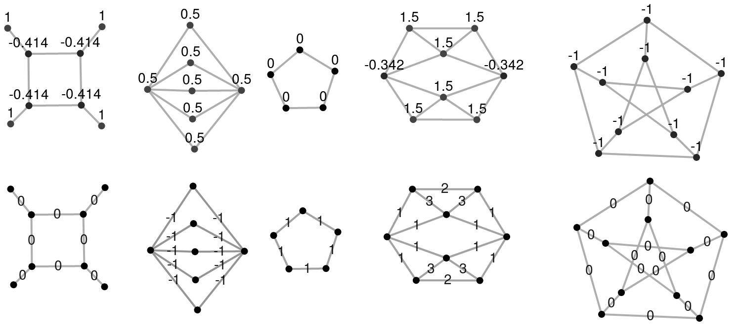
Figure 1: The upper row shows the non-normalized Bakry-Emery curvature. The lower row shows the non-normalized Ollivier curvature from [MW17]. The curvature was calculated by the graph curvature calculator [CKL⁺17].

As demonstrated in Figure 1, there is no implication between non-negative Bakry-Emery and non-negative Ollivier curvature. We remark that Bakry-Emery and Ollivier curvature are intrinsically different in the sense that Ollivier curvature is defined on edges and Bakry Emery curvature is defined on vertices and can be considered as an analog of the minimal eigenvalue of the Ricci curvature tensor in a point. Moreover in this paper, we refer to Lin-Lu-Yau’s modification of Ollivier curvature which corresponds to lazy random walks and is always larger or equal to Ollivier curvature for non-lazy random walks, see [LLY11].

Although there are no results yet known for non-negative Ollivier curvature, the case of positive Ollivier curvature is well understood. In particular, a positive lower bound on the Ollivier curvature implies an upper diameter bound, eigenvalue estimates, and concentration of the measure [Oll09, BJL12]. In this note, we improve the concentration of the measure by applying the methods from [Sch98].

1.1 Setup and notation

A measured and weighted graph $G=(V,w,m)$ is triple consisting of a countable set $V$, a symmetric function $w:V\times V\to[0,\infty)$ which is zero on the diagonal, and a function $m:V\to(0,\infty)$. We write $x\sim y$ whenever $w(x,y)>0$. We will always assume local finiteness, i.e., for all $x\in V$,

$$|\{y:w(x,y)>0\}|<\infty.$$

We write $q(x,y):=w(x,y)/m(x)$ and define $\Delta:\mathbb{R}^{V}\to\mathbb{R}^{V}$ by

$$\Delta f(x):=\sum_{y}q(x,y)(f(y)-f(x)).$$

Note that $\Delta\leq 0$, i.e., $\sum_{x}m(x)f(x)\Delta f(x)\leq 0$ for all finitely supported $f:V\to\mathbb{R}$. We say a function $f\in\mathbb{R}^{V}$ is harmonic if $\Delta f=0$. We denote the weighted vertex degree of $x\in V$ by $\operatorname{Deg}(x):=\sum_{y}q(x,y)$, see e.g. [HKMW13, Section 2.2]. In the Markov chain setting, the weighted vertex degree is usually called jump rate $J(x)$, see e.g. [FS18]. We write

$$\operatorname{Deg}_{\max}:=\sup_{x\in V}\operatorname{Deg}(x)\qquad\mbox{ and }\qquad q_{\min}:=\inf_{x\sim y}q(x,y).$$

The combinatorial graph distance is given by

$$d(x,y):=\inf\{n:x=x_{0}\sim\ldots\sim x_{n}=y\}.$$

Given the graph distance, we define the gradient $\nabla_{xy}f$ for $f\in\mathbb{R}^{V}$ and $x\neq y\in V$ via

$$\nabla_{xy}f:=\frac{f(x)-f(y)}{d(x,y)}.$$

for $f\in\mathbb{R}^{V}$, we write $\|f\|_{\infty}:=\sup_{x\in V}|f(x)|$ and

$$\|\nabla f\|_{\infty}:=\sup_{x\sim y}\nabla_{xy}f.$$

The Ollivier curvature, also called coarse Ricci curvature, was introduced in [Oll07, Oll09] for discrete Markov chains. Modifications have been given defined in [LLY11] and [JL14] in order to compute the curvature of random graphs and to relate curvature to the clustering coefficient. In this article, we use the generalized version of Ollivier curvature from [MW17] which is applicable to all weighted graph Laplacians. By [MW17], the Ollivier curvature $\kappa(x,y)$ for $x\neq y\in V$ is given by

$$\kappa(x,y):=\inf_{\begin{subarray}{c}\nabla_{yx}f=1\\ \|\nabla f\|_{\infty}=1\end{subarray}}\nabla_{xy}\Delta f.$$

This definition coincides with the modified curvature introduced by Lin, Lu, Yau [LLY11] whenever the latter is defined, i.e., whenever $\operatorname{Deg}\equiv 1$ and $w(x,y)\in\{0,1\}$, see [MW17, Theorem 2.1]. By [MW17, Proposition 2.4], the curvature can also be calculated via transport plans. Connecting the Lipschitz functions to optimal transport plans is a crucial step for proving the Liouville property. Therefore, we recall [MW17, Proposition 2.4].

Proposition 1.1 (See [MW17, Proposition 2.4]).

Let $G=(V,w,m)$ be a graph and let $x_{0}\neq y_{0}$ be vertices. Then,

$$\kappa(x_{0},y_{0}) =\sup_{\rho}\sum_{\begin{subarray}{c}x\in B_{1}(x_{0})\\ y\in B_{1}(y_{0})\end{subarray}}\rho(x,y)\left[1-\frac{d(x,y)}{d(x_{0},y_{0})}\right]$$ (1)

where the supremum is taken over all $\rho:B_{1}(x_{0})\times B_{1}(y_{0})\to[0,\infty)$ such that

$$\sum_{y\in B_{1}(y_{0})}\rho(x,y) =q(x_{0},x)\qquad\mbox{ for all }x\in S_{1}(x_{0})\mbox{ and}$$ (2)

$$\sum_{x\in B_{1}(x_{0})}\rho(x,y) =q(y_{0},y)\qquad\mbox{ for all }y\in S_{1}(y_{0}).$$ (3)

We remark that $\rho$ is defined on balls, but we only require the coupling property on spheres. Moreover, we do no not assume that $\rho$ is a probability measure. A function $\rho$ attaining the supremum in (1) is called optimal transport plan. Due to compactness, there always exists an optimal transport plan.

2 Liouville property and non-negative Ollivier curvature

The study of harmonic functions and, in particular, the Liouville property on manifolds with non-negative Ricci curvature traces back to [Yau75] and is still matter of current research [CMW19]. Liouville type properties on graphs have been studied in e.g. [Woe00, Mas09, BS96]. We now present our main theorem stating that every bounded harmonic function is constant when assuming non-negative Ollivier curvature.

Theorem 2.1.

Let $G=(V,w,m)$ be a graph. Suppose

• $\operatorname{Deg}_{\max}<\infty$,

• $q_{\min}>0$,

• $\kappa(x,y)\geq 0$ for all $x\neq y\in V$.

Then, every bounded harmonic function is constant.

We remark that the assumption $\kappa(x,y)\geq 0$ is weaker than assuming non-negative Ollivier curvature in the non-lazy random walk setting. In order to prove the theorem, we first need a lemma concerning transport plans, stating that if $\kappa(x_{0},y_{0})\leq\varepsilon$, then there exists an optimal transport plan which transports a significant amount of mass over the distance $d(x_{0},y_{0})+1$.

Lemma 2.2.

Suppose $d(x_{0},y_{0})\kappa(x_{0},y_{0})\leq\varepsilon$ for some $x_{0},y_{0}\in V$ and some $\varepsilon>0$. Then, there exists an optimal transport plan $\rho:B_{1}(x_{0})\times B_{1}(y_{0})\to[0,\infty)$ s.t.

$$\sum_{\begin{subarray}{c}x\in B_{1}(x_{0})\\ y\in B_{1}(y_{0})\\ d(x,y)>d(x_{0},y_{0})\end{subarray}}\rho(x,y)\geq(q_{\min}-\varepsilon)/2.$$

Remarkably, this lemma fails in the non-lazy random walk setting as one can see on the one-dimensional lattice $\mathbb{Z}$ with standard weights.

Proof.

Let $\rho_{0}$ be an optimal transport plan and let $x^{\prime}\sim x_{0}$ s.t. $d(x^{\prime},y_{0})=d(x_{0},y_{0})-1$. We want to construct an optimal transport plan transporting a significant mass over the distance $d(x_{0},y_{0})+1$. To this end, we construct an optimal transport plan transporting a significant amount of mass over a distance shorter than $d(x_{0},y_{0})$ which will be useful since the average transport distance is close to $d(x_{0},y_{0})$ if the curvature is small. In particular, our transport plan will have the property that $x^{\prime}$ is transported only to vertices $y\in B_{1}(y_{0})$ with $d(x^{\prime},y)\leq d(x_{0},y_{0})-1$. We define a map $\rho:B_{1}(x_{0})\times B_{1}(y_{0})\to[0,\infty)$ which shall be our new optimal transport plan via

$$\rho(x,y):=\begin{cases}\rho_{0}(x,y_{0})+\sum_{\begin{subarray}{c}z\in B_{1}(y_{0})\\ d(x^{\prime},z)\geq d(x_{0},y_{0})\end{subarray}}\rho_{0}(x^{\prime},z)&:x=x^{\prime},y=y_{0},\\ 0&:x=x^{\prime},d(x^{\prime},y)\geq d(x_{0},y_{0}),\\ \rho_{0}(x_{0},y)+\rho_{0}(x^{\prime},y)&:x=x_{0},d(x^{\prime},y)\geq d(x_{0},y_{0}),\\ \rho_{0}(x,y)&:\mbox{otherwise}.\end{cases}$$

We now prove that $\rho$ is also an optimal transport plan. To this end, we first show that $\rho$ satisfies the marginal conditions. For $x=x^{\prime}$, we have

$$\sum_{y\in B_{1}(y_{0})}\rho(x^{\prime},y) =\rho(x^{\prime},y_{0})+\sum_{d(x^{\prime},y)\geq d(x_{0},y_{0})}\rho(x^{\prime},y)+\sum_{\begin{subarray}{c}d(x^{\prime},y)<d(x_{0},y_{0})\\ y\neq y_{0}\end{subarray}}\rho(x^{\prime},y)$$

$$=\left(\rho_{0}(x^{\prime},y_{0})+\sum_{d(x^{\prime},y)\geq d(x_{0},y_{0})}\rho_{0}(x^{\prime},y)\right)+0+\sum_{\begin{subarray}{c}d(x^{\prime},y)<d(x_{0},y_{0})\\ y\neq y_{0}\end{subarray}}\rho_{0}(x^{\prime},y)$$

$$=\sum_{y\in B_{1}(y_{0})}\rho_{0}(x^{\prime},y)$$

$$=q(x_{0},x^{\prime}).$$

For $x\in S_{1}(x_{0})\setminus\{x^{\prime}\}$, we have $\rho(x,y)=\rho_{0}(x,y)$ for all $y\in B_{1}(y_{0})$, and thus,

$$\sum_{y\in B_{1}(y_{0})}\rho(x,y)=\sum_{y\in B_{1}(y_{0})}\rho_{0}(x,y)=q(x_{0},x).$$

For $y\in S_{1}(y_{0})$ s.t. $d(x^{\prime},y)<d(x_{0},y_{0})$, we have $\rho(x,y)=\rho_{0}(x,y)$ for all $x\in B_{1}(x_{0})$, and thus,

$$\sum_{x\in B_{1}(x_{0})}\rho(x,y)=\sum_{x\in B_{1}(x_{0})}\rho_{0}(x,y)=q(y_{0},y).$$

For $y\in S_{1}(y_{0})$ s.t. $d(x^{\prime},y)\geq d(x_{0},y_{0})$, we have

$$\sum_{x\in B_{1}(x_{0})}\rho(x,y) =\rho(x_{0},y)+\rho(x^{\prime},y)+\sum_{x\in S_{1}(x_{0})\setminus\{x^{\prime}\}}\rho(x,y)$$

$$=\Big{(}\rho_{0}(x_{0},y)+\rho_{0}(x^{\prime},y)\Big{)}+0+\sum_{x\in S_{1}(x_{0})\setminus\{x^{\prime}\}}\rho_{0}(x,y)$$

$$=\sum_{x\in B_{1}(x_{0})}\rho_{0}(x,y)=q(y_{0},y).$$

This proves that $\rho$ is indeed a transport plan. In order to show that $\rho$ is optimal, it is sufficient by optimality of $\rho_{0}$ to show

$$\sum_{\begin{subarray}{c}x\in B_{1}(x_{0})\\ y\in B_{1}(y_{0})\end{subarray}}\rho(x,y)\Big{(}d(x_{0},y_{0})-d(x,y)\Big{)}\geq\sum_{\begin{subarray}{c}x\in B_{1}(x_{0})\\ y\in B_{1}(y_{0})\end{subarray}}\rho_{0}(x,y)\Big{(}d(x_{0},y_{0})-d(x,y)\Big{)}$$

We write $C(x,y):=\Big{(}\rho(x,y)-\rho_{0}(x,y)\Big{)}\Big{(}d(x_{0},y_{0})-d(x,y)\Big{)}$. Thus, it suffices to prove

$$\sum_{\begin{subarray}{c}x\in B_{1}(x_{0})\\ y\in B_{1}(y_{0})\end{subarray}}C(x,y)\geq 0.$$

Since $C(x,y)=0$ whenever $\rho(x,y)=\rho_{0}(x,y)$, we have

$$\sum_{\begin{subarray}{c}x\in B_{1}(x_{0})\\ y\in B_{1}(y_{0})\end{subarray}}C(x,y)=C(x^{\prime},y_{0})+\sum_{d(x^{\prime},y)\geq d(x_{0},y_{0})}\Big{(}C(x^{\prime},y)+C(x_{0},y)\Big{)}.$$

Observe that since $\rho(x^{\prime},y)=0$ whenever $d(x^{\prime},y)\geq d(x_{0},y_{0})$, we have

$$C(x^{\prime},y_{0})=\left(\sum_{d(x^{\prime},y)\geq d(x_{0},y_{0})}\rho_{0}(x^{\prime},y)\right)\cdot\Big{(}d(x_{0},y_{0})-d(x^{\prime},y_{0})\Big{)}=\sum_{d(x^{\prime},y)\geq d(x_{0},y_{0})}\rho_{0}(x^{\prime},y).$$

If $d(y,x^{\prime})\geq d(x_{0},y_{0})$, we have

$$C(x^{\prime},y)=-\rho_{0}(x^{\prime},y)\Big{(}d(x_{0},y_{0})-d(x^{\prime},y)\Big{)}$$

and

$$C(x_{0},y)=\rho_{0}(x^{\prime},y)\Big{(}d(x_{0},y_{0})-d(x_{0},y)\Big{)}$$

and thus,

$$C(x^{\prime},y)+C(x_{0},y)=\rho_{0}(x^{\prime},y)\Big{(}d(x^{\prime},y)-d(x_{0},y)\Big{)}\geq-\rho_{0}(x^{\prime},y)$$

since $|d(x^{\prime},y)-d(x_{0},y)|\leq d(x_{0},x^{\prime})=1$. Putting together gives

$$\sum_{\begin{subarray}{c}x\in B_{1}(x_{0})\\ y\in B_{1}(y_{0})\end{subarray}}C(x,y) =C(x^{\prime},y_{0})+\sum_{d(x^{\prime},y)\geq d(x_{0},y_{0})}\Big{(}C(x^{\prime},y)+C(x_{0},y)\Big{)}$$

$$\geq\sum_{d(x^{\prime},y)\geq d(x_{0},y_{0})}\rho_{0}(x^{\prime},y)-\sum_{d(x^{\prime},y)\geq d(x_{0},y_{0})}\rho_{0}(x^{\prime},y)=0$$

which proves that $\rho$ is an optimal transport plan. Observe that via the transport plan $\rho$ the vertex $x^{\prime}$ is transported only to vertices $y$ with $d(x^{\prime},y)<d(x_{0},y_{0})$, i.e.,

$$q(x_{0},x^{\prime})=\sum_{y}\rho(x^{\prime},y)=\sum_{d(x^{\prime},y)<d(x_{0},y_{0})}\rho(x^{\prime},y).$$

Thus, we have

$$\varepsilon\geq d(x_{0},y_{0})\kappa(x_{0},y_{0}) =\sum_{\begin{subarray}{c}x\in B_{1}(x_{0})\\ y\in B_{1}(y_{0})\end{subarray}}\rho(x,y)(d(x_{0},y_{0})-d(x,y))$$

$$\geq\sum_{\begin{subarray}{c}x\in B_{1}(x_{0})\\ y\in B_{1}(y_{0})\\ d(x,y)<d(x_{0},y_{0})\end{subarray}}\rho(x,y)-2\cdot\sum_{\begin{subarray}{c}x\in B_{1}(x_{0})\\ y\in B_{1}(y_{0})\\ d(x,y)>d(x_{0},y_{0})\end{subarray}}\rho(x,y)$$

$$\geq\sum_{\begin{subarray}{c}y\in B_{1}(y_{0})\\ d(x,y)<d(x_{0},y_{0})\end{subarray}}\rho(x^{\prime},y)-2\cdot\sum_{\begin{subarray}{c}x\in B_{1}(x_{0})\\ y\in B_{1}(y_{0})\\ d(x,y)>d(x_{0},y_{0})\end{subarray}}\rho(x,y)$$

$$=q(x_{0},x^{\prime})-2\cdot\sum_{\begin{subarray}{c}x\in B_{1}(x_{0})\\ y\in B_{1}(y_{0})\\ d(x,y)>d(x_{0},y_{0})\end{subarray}}\rho(x,y)$$

where the second estimate follows from $d(x_{0},y_{0})-d(x,y)\in\{-2,-1,0,1,2\}$.

Hence,

$$\sum_{\begin{subarray}{c}x\in B_{1}(x_{0})\\ y\in B_{1}(y_{0})\\ d(x,y)>d(x_{0},y_{0})\end{subarray}}\rho(x,y)\geq(q(x_{0},x^{\prime})-\varepsilon)/2\geq(q_{\min}-\varepsilon)/2.$$

This finishes the proof. ∎

For simplicity, we write $D:=\operatorname{Deg}_{\max}$ and $q:=q_{\min}$.

Lemma 2.3.

Let $f$ be a harmonic function with $\|\nabla f\|_{\infty}=1$. Let $\varepsilon\in(0,q/4D)$ and let $x_{0}\neq y_{0}$ s.t. $f(x_{0})-f(y_{0})\geq d(x_{0},y_{0})-\varepsilon$. Then, there exists $x^{\prime}\in B_{1}(x_{0})$ and $y^{\prime}\in B_{1}(y_{0})$ s.t.

• $f(x^{\prime})-f(y^{\prime})>d(x^{\prime},y^{\prime})-\varepsilon\cdot 10D/q$,

• $d(x^{\prime},y^{\prime})>d(x_{0},y_{0})$.

Proof.

Define $g_{0}:B_{1}(x_{0})\to\mathbb{R}$ via

$$g_{0}(w):=f(w)\wedge(f(x_{0})-d(x_{0},y_{0})+d(y_{0},w)).$$

Then, $g_{0}$ is $1$-Lipschitz as the minimum of two $1$-Lipschitz functions. Let $g:V\to\mathbb{R}$ the minimal Lipschitz extension of $g_{0}$ given by

$$g(z):=\max_{w\in B_{1}(x_{0})}g_{0}(w)-d(w,z).$$

For all $z\in V$ and all $w\in B_{1}(x_{0})$, the condition $\|\nabla f\|_{\infty}=1$ yields

$$f(z)\geq f(w)-d(z,w)\geq g_{0}(w)-d(z,w)$$

which implies $f\geq g$. Since $g_{0}$ is $1$-Lipschitz, we have $g_{0}=g|_{B_{1}(x_{0})}$. Observe that $g$ is $1$-Lipschitz as a maximum of $1$-Lipschitz functions. Thus, $g(y_{0})\geq g(x_{0})-d(x_{0},y_{0})$. On the other hand, we have

$$g(y_{0})\leq\max_{w\in B_{1}(x_{0})}\Big{(}f(x_{0})-d(x_{0},y_{0})+d(y_{0},w)\Big{)}-d(w,y_{0})=f(x_{0})-d(x_{0},y_{0}).$$

Since $f(x_{0})=g_{0}(x_{0})=g(x_{0})$, we obtain $g(y_{0})\leq f(x_{0})-d(x_{0},y_{0})=g(x_{0})-d(x_{0},y_{0})\leq g(y_{0})$ implying $g(y_{0})=g(x_{0})-d(x_{0},y_{0})$. Moreover for $w\in B_{1}(x_{0})$,

$$f(x_{0})-d(x_{0},y_{0})+d(y_{0},w)\geq f(y_{0})-\varepsilon+d(y_{0},w)\geq f(w)-\varepsilon$$

yielding $g(w)=g_{0}(w)\geq f(w)-\varepsilon$. Thus, $\Delta g(x_{0})\geq\Delta f(x_{0})-D\varepsilon$ by the definition of $\Delta$. Since $g(y_{0})=f(x_{0})-d(x_{0},y_{0})\geq f(y_{0})-\varepsilon$ and since $g\leq f$, we have $\Delta g(y_{0})\leq\Delta f(y_{0})+D\varepsilon$. Since $\nabla_{x_{0}y_{0}}g=\|\nabla g\|_{\infty}=1$, the definition of $\kappa$ gives

$$d(x_{0},y_{0})\kappa(x_{0},y_{0})\leq\Delta g(y_{0})-\Delta g(x_{0})\leq 2D\varepsilon.$$

We have $g(y)-g(x)\geq-d(x,y)$. Let

$$H:=\min_{\begin{subarray}{c}x\in B_{1}(x_{0})\\ y\in B_{1}(y_{0})\\ d(x,y)>d(x_{0},y_{0})\end{subarray}}d(x,y)-g(x)+g(y)\geq 0$$

where the set from which the minimum is taken is not empty due to Lemma 2.2 and finite due to local finiteness. Let $\rho$ be the optimal transport plan from Lemma 2.2. We write

$$2D\varepsilon\geq\Delta g(y_{0})-\Delta g(x_{0}) \geq\sum_{\begin{subarray}{c}x\in B_{1}(x_{0})\\ y\in B_{1}(y_{0})\end{subarray}}\rho(x,y)(g(y)-g(y_{0}))-\sum_{\begin{subarray}{c}x\in B_{1}(x_{0})\\ y\in B_{1}(y_{0})\end{subarray}}\rho(x,y)(g(x)-g(x_{0}))$$

$$=\sum_{\begin{subarray}{c}x\in B_{1}(x_{0})\\ y\in B_{1}(y_{0})\end{subarray}}\rho(x,y)(g(y)-g(x)+d(x_{0},y_{0}))$$

$$\geq\sum_{\begin{subarray}{c}x\in B_{1}(x_{0})\\ y\in B_{1}(y_{0})\end{subarray}}\rho(x,y)(d(x_{0},y_{0})-d(x,y))+\sum_{\begin{subarray}{c}x\in B_{1}(x_{0})\\ y\in B_{1}(y_{0})\\ d(x,y)>d(x_{0},y_{0})\end{subarray}}\rho(x,y)(d(x,y)-g(x)+g(y))$$

$$\geq d(x_{0},y_{0})\kappa(x_{0},y_{0})+H\sum_{\begin{subarray}{c}x\in B_{1}(x_{0})\\ y\in B_{1}(y_{0})\\ d(x,y)>d(x_{0},y_{0})\end{subarray}}\rho(x,y)$$

$$\geq H(q-2D\varepsilon)/2$$

where the last estimate follows from Lemma 2.2. Hence, $H\leq\frac{4D\varepsilon}{q-2D\varepsilon}$. In particular, there exists $x^{\prime}\in B_{1}(x_{0})$ and $y^{\prime}\in B_{1}(y_{0})$ with $d(x^{\prime},y^{\prime})>d(x_{0},y_{0})$ s.t.

$$g(x^{\prime})-g(y^{\prime})\geq d(x^{\prime},y^{\prime})-\frac{4D\varepsilon}{q-2D\varepsilon}\geq d(x^{\prime},y^{\prime})-8D\varepsilon/q$$

where the last estimate follows from $\varepsilon<\frac{q}{4D}$. We now show that $g$ approximates $f$ in order to lower bound $f(x^{\prime})-f(y^{\prime})$. We have $g(x^{\prime})\leq f(x^{\prime})$ and

$$-D\varepsilon\leq\Delta g(x_{0})\leq\Delta g(y_{0})=\Delta g(y_{0})-\Delta f(y_{0}) =D(f(y_{0})-g(y_{0}))-\sum_{y\sim y_{0}}q(y_{0},y)(f(y)-g(y))$$

$$\leq D\varepsilon-q(y_{0},y^{\prime})(f(y^{\prime})-g(y^{\prime})).$$

Thus,

$$f(y^{\prime})\leq g(y^{\prime})+2D\varepsilon/q(y_{0},y^{\prime})\leq g(y^{\prime})+2D\varepsilon/q.$$

Putting together gives

$$f(x^{\prime})-f(y^{\prime})\geq g(x^{\prime})-g(y^{\prime})-2D\varepsilon/q\geq d(x^{\prime},y^{\prime})-\varepsilon\cdot 10D/q.$$

This finishes the proof. ∎

We recall $D=\operatorname{Deg}_{\max}$ and $q=q_{\min}$.

Proof of Theorem 2.1.

Let $f$ be a bounded harmonic function. Then, $\|\nabla f\|_{\infty}<\infty$. If $f$ is not constant, we can assume $\|\nabla f\|_{\infty}=1$ without obstruction. Let $2\|f\|_{\infty}<N\in\mathbb{N}$. Let $\varepsilon<\left(\frac{q}{10D}\right)^{N}$ be small. Let $x_{0}\sim y_{0}$ s.t. $\nabla f(x_{0},y_{0})>1-\varepsilon$. We inductively apply Lemma 2.3 to construct sequences $(x_{n})_{n=0}^{N}$ and $(y_{n})_{n=0}^{N}$ with the following properties:

• $d(x_{n},y_{n})\geq n+1$,

• $f(x_{n})-f(y_{n})\geq d(x_{n},y_{n})-\varepsilon\cdot(10D/q)^{n}$.

In particular given $x_{n}$ and $y_{n}$, we have $d(x_{n},y_{n})\geq n+1$ and $f(x_{n})-f(y_{n})\geq d(x_{n},y_{n})-\varepsilon\cdot(10D/q)^{n}$ by the induction hypothesis. We now apply Lemma 2.3 to obtain $x^{\prime},y^{\prime}$ with $d(x^{\prime},y^{\prime})>d(x_{n},y_{n})$ and

$$f(x^{\prime})-f(y^{\prime})\geq d(x^{\prime},y^{\prime})-\left(\varepsilon\cdot(10D/q)^{n}\right)\cdot 10D/Q=d(x^{\prime},y^{\prime})-\varepsilon\cdot(10D/q)^{n+1}.$$

Thus we set $x_{n+1}:=x^{\prime}$ and $y_{n+1}:=y^{\prime}$ which satisfy the desired properties. In particular,

$$\|f\|_{\infty}+\|f\|_{\infty}\geq f(x_{N})-f(y_{N})>d(x_{N},y_{N})-1\geq N+1-1>2\|f\|_{\infty}.$$

This is a contradiction, and thus, $f$ is constant. This finishes the proof. ∎

3 Concentration of measure

We apply the methods from [Sch98] to improve the concentration of measure results by Ollivier [Oll09]. In [Sch98], concentration of measure is proved under a positive Bakry Emery curvature bound. For

$$f\in\ell^{1}(V,m):=\{g\in C(V):\sum_{x\in V}m(x)|g(x)|<\infty\}$$

we write

$$\langle g\rangle:=\sum_{x\in V}m(x)g(x).$$

We now state our concentration theorem which gives a Gaussian upper bound for the measure of the vertices for which a Lipschitz function deviates from its mean more than $r$. Non-explicit concentration bounds via transport-information inequalities in terms of Ollivier curvature can also be found in [FS18].

Theorem 3.1.

Let $G=(V,w,m)$ be a graph and let $K>0$. Suppose

• $\operatorname{Deg}_{\max}\leq 1$,

• $m(V)=1$,

• $\kappa(x,y)\geq K>0$ for all $x\neq y\in V$.

Let $f\in\ell^{1}(V,m)$ s.t.

• $\langle f\rangle=0$,

• $\|\nabla f\|_{1}\leq 1$.

Then,

$$m(f>r)\leq e^{-{Kr^{2}}}.$$

This improves the concentration result by Ollivier [Oll09, Theorem 33] roughly stating that under the same assumptions as in the theorem,

$$m(f>r)\leq e^{-{K^{2}r^{2}}}$$

if $r$ is not too large. Firstly, having $K$ in the exponent is better than $K^{2}$ up to a constant since $K\leq 2$ due to $\operatorname{Deg}_{\max}\leq 1$. Secondly, our concentration result holds without restricting to small enough $r$.

Proof.

We first observe that $G$ has finite diameter due to [MW17, Proposition 4.14]. Thus, $G$ is finite due to local finiteness. Following [Sch98], we have

$$-\partial_{t}\langle e^{\lambda P_{t}f}\rangle=-\langle\lambda\Delta P_{t}f,e^{\lambda P_{t}f}\rangle=\langle\Gamma(\lambda P_{t}f,e^{\lambda P_{t}f})\rangle\leq\lambda^{2}\langle e^{\lambda P_{t}f},\Gamma(P_{t}f)\rangle$$

where $2\Gamma(g,h):=\Delta(fg)-f\Delta g-g\Delta f$. Moreover by [MW17, Theorem 3.8], and since $\operatorname{Deg}_{\max}\leq 1$,

$$2\Gamma(P_{t}f)\leq\|\nabla P_{t}f\|_{\infty}^{2}\leq e^{-2Kt}\|\nabla f\|_{\infty}^{2}\leq e^{-2Kt}.$$

Putting together gives

$$-\partial_{t}\langle e^{\lambda P_{t}f}\rangle\leq\frac{\lambda^{2}}{2}e^{-2Kt}\langle e^{\lambda P_{t}f}\rangle.$$

Integrating from $t=0$ to $\infty$ and applying $\lim_{t\to\infty}e^{\lambda P_{t}f}=1$ gives

$$\langle e^{\lambda f}\rangle\leq e^{\frac{\lambda^{2}}{4K}}.$$

Thus, we have

$$m(f>r)\leq e^{-\lambda r}\langle e^{\lambda f}\rangle\leq\exp\left(\frac{\lambda^{2}}{4K}-\lambda r\right)=\exp\left(-{Kr^{2}}\right)$$

when choosing $\lambda=2rK$. This finishes the proof. ∎

References

• [BHL+15] Frank Bauer, Paul Horn, Yong Lin, Gabor Lippner, Dan Mangoubi, Shing-Tung Yau, et al. Li-Yau inequality on graphs. Journal of Differential Geometry, 99(3):359–405, 2015.
• [BJL12] Frank Bauer, Jürgen Jost, and Shiping Liu. Ollivier-Ricci curvature and the spectrum of the normalized graph Laplace operator. Mathematical Research Letters, 19(6):1185–1205, 2012.
• [BS96] Itai Benjamini and Oded Schramm. Harmonic functions on planar and almost planar graphs and manifolds, via circle packings. Inventiones mathematicae, 126(3):565–587, 1996.
• [CKL+17] David Cushing, Riikka Kangaslampi, Valtteri Lipiäinen, Shiping Liu, and George William Stagg. The Graph Curvature Calculator and the curvatures of cubic graphs. arXiv preprint arXiv:1712.03033, 2017.
• [CLY14] Fan Chung, Yong Lin, and S-T Yau. Harnack inequalities for graphs with non-negative Ricci curvature. Journal of Mathematical Analysis and Applications, 415(1):25–32, 2014.
• [CMW19] Tobias Holck Colding, II Minicozzi, and P William. Liouville properties. arXiv preprint arXiv:1902.09366, 2019.
• [DKZ17] Dominik Dier, Moritz Kassmann, and Rico Zacher. Discrete versions of the Li-Yau gradient estimate. arXiv preprint arXiv:1701.04807, 2017.
• [FS18] Max Fathi and Yan Shu. Curvature and transport inequalities for Markov chains in discrete spaces. Bernoulli, 24(1):672–698, 2018.
• [GL17] Chao Gong and Yong Lin. Equivalent properties for CD inequalities on graphs with unbounded Laplacians. Chin. Ann. Math. Ser. B, 38(5):1059–1070, 2017.
• [HKMW13] Xueping Huang, Matthias Keller, Jun Masamune, and Radosław K. Wojciechowski. A note on self-adjoint extensions of the Laplacian on weighted graphs. Journal of Functional Analysis, 265(8):1556–1578, 2013.
• [HLLY17] Paul Horn, Yong Lin, Shuang Liu, and Shing-Tung Yau. Volume doubling, Poincaré inequality and Gaussian heat kernel estimate for non-negatively curved graphs. Journal für die reine und angewandte Mathematik (Crelles Journal), 2017.
• [Hua17] Bobo Hua. Liouville theorem for bounded harmonic functions on graphs satisfying non-negative curvature dimension condition. arXiv preprint arXiv:1702.00961, 2017.
• [JL14] Jürgen Jost and Shiping Liu. Ollivier’s Ricci curvature, local clustering and curvature-dimension inequalities on graphs. Discrete & Computational Geometry, 51(2):300–322, 2014.
• [KKRT16] Bo’az Klartag, Gady Kozma, Peter Ralli, and Prasad Tetali. Discrete curvature and abelian groups. Canad. J. Math., 68(3):655–674, 2016.
• [KM18] Matthias Keller and Florentin Münch. Gradient estimates, Bakry-Emery Ricci curvature and ellipticity for unbounded graph Laplacians. arXiv preprint arXiv:1807.10181, 2018.
• [Liu18] Shuang Liu. Buser’s inequality on infinite graphs. arXiv preprint arXiv:1810.12003, 2018.
• [LL15] Yong Lin and Shuang Liu. Equivalent properties of CD inequality on graph. arXiv preprint arXiv:1512.02677, 2015.
• [LLY11] Yong Lin, Linyuan Lu, and Shing-Tung Yau. Ricci curvature of graphs. Tohoku Mathematical Journal, Second Series, 63(4):605–627, 2011.
• [LMP15] Shiping Liu, Florentin Münch, and Norbert Peyerimhoff. Curvature and higher order Buser inequalities for the graph connection Laplacian. arXiv preprint arXiv:1512.08134, 2015.
• [LP18] Shiping Liu and Norbert Peyerimhoff. Eigenvalue Ratios of Non-Negatively Curved Graphs. Combinatorics, Probability and Computing, pages 1–22, 2018.
• [Mas09] Jun Masamune. A Liouville property and its application to the Laplacian of an infinite graph. Contemporary Mathematics, 484:103, 2009.
• [Mün17] Florentin Münch. Remarks on curvature dimension conditions on graphs. Calculus of Variations and Partial Differential Equations, 56(1):11, 2017.
• [Mün18] Florentin Münch. Li-Yau inequality on finite graphs via non-linear curvature dimension conditions. Journal de Mathématiques Pures et Appliquées, 120:130–164, 2018.
• [MW17] Florentin Münch and Radoslaw K Wojciechowski. Ollivier Ricci curvature for general graph Laplacians: Heat equation, Laplacian comparison, non-explosion and diameter bounds. arXiv preprint arXiv:1712.00875, 2017.
• [Oll07] Yann Ollivier. Ricci curvature of metric spaces. Comptes Rendus Mathematique, 345(11):643–646, 2007.
• [Oll09] Yann Ollivier. Ricci curvature of Markov chains on metric spaces. Journal of Functional Analysis, 256(3):810–864, 2009.
• [Sch98] Michael Schmuckenschläger. Curvature of nonlocal Markov generators. Convex geometric analysis (Berkeley, CA, 1996), 34:189–197, 1998.
• [Woe00] Wolfgang Woess. Random walks on infinite graphs and groups, volume 138. Cambridge university press, 2000.
• [Yau75] Shing-Tung Yau. Harmonic functions on complete Riemannian manifolds. Communications on Pure and Applied Mathematics, 28(2):201–228, 1975.