Stacked Monte Carlo for option pricing

Abstract.

We introduce a stacking version of the Monte Carlo algorithm in the context of option pricing. Introduced recently for aeronautic computations, this simple technique, in the spirit of current machine learning ideas, learns control variates by approximating Monte Carlo draws with some specified function. We describe the method from first principles and suggest appropriate fits, and show its efficiency to evaluate European and Asian Call options in constant and stochastic volatility models.

1. Introduction

Monte Carlo methods are the most fundamental pillar for pricing models in quantitative finance, and a considerable amount effort has been made to refine their properties, from variance reduction techniques [18, Chapter 4] (importance sampling, antithetic variables or control variates) to discretisation of stochastic differential equations [28] and their multilevel extensions [15, 16, 17]. Indeed, most financial instruments do not admit closed-form pricing formulae, and any numerical technique is thus at the mercy of instabilities and approximation errors. This of course generated an appetite for variance reduction techniques, whereby more stability can be achieved with similar computation time and level of accuracy. There has recently also been a lot of interest in leveraging the power of machine learning tools, mainly on the use of neural networks to solve pricing [10, 13, 30, 19, 24, 29] and calibration [6, 23, 32] problems.

We consider here an alternative approach, which involves the application of simple regression techniques to improve Monte Carlo estimates. We borrow the idea from Alonso, Tracey and Wolpert [4, 33] who were first motivated by applications in aeronautics. The main idea is to learn appropriate control variates for option pricing problems, in order to achieve high levels of variance reduction. This task faces two challenges; the first is to obtain unbiased estimates of the pricing payoff function, as the Stacked Monte Carlo technique proposed in [4, 33] did not apply to derivatives pricing. The second challenge is to select the appropriate fitting functions for our pricing problems, such that the model closely approximates the solution whilst being sufficiently simple to minimise computation times. We start below by presenting the stacked Monte Carlo in its simple form, namely to numerically compute integrals, before applying it pricing options in the Black-Scholes and in the Heston model. We shall consider European options as well as Asian options, showing how to adapt the method to multivariate problems. We then carry out numerical tests highlighting both the simplicity and the efficiency of the method.

2. Stacked Monte Carlo

The Stacked Monte Carlo (StackMC) method [4, 33], is a post-processing technique for reducing the error in Monte Carlo estimates. The main idea is to learn a control variate from the Monte Carlo draws, such that the distribution of the learnt function approximates that of the original problem. While doing so, it is crucial to avoid bias and overfitting, as this may worsen the final result. We rewrite the solution to a Monte Carlo problem $f(x)$ in terms a learnt function $g(x)$

(1) $$\widehat{f}=\int{f(x)p(x)\mathrm{d}x}=\int{\alpha g(x)p(x)\mathrm{d}x}+\int{\left[f(x)-\alpha g(x)\right]p(x)}=\alpha\widehat{g}+\int{\left[f(x)-\alpha g(x)\right]p(x)},$$

where $\alpha$ is some constant and $\widehat{g}:=\int{g(x)p(x)\mathrm{d}x}$. If $g$ is a reasonable fit to $f$, the difference $f-\alpha g$ for some appropriately chosen $\alpha$ will have lower variance than the original problem. Over the observations $(x^{(i)})_{i=1,\ldots,N}$, the estimate

(2) $$\widetilde{f}:=\alpha\widehat{g}+\frac{1}{N}\sum_{i=1}^{N}\left[f\left(x^{(i)}\right)-\alpha g\left(x^{(i)}\right)\right]$$

has variance $\sigma^{2}_{\widetilde{f}}=\sigma^{2}_{f}+\alpha^{2}\sigma^{2}_{g}-2\alpha\sigma_{f,g}$ which is minimised as soon as

(3) $$\alpha=\frac{\sigma_{f}}{\sigma_{g}}\rho_{f,g},$$

which implies $\sigma^{2}_{\widetilde{f}}=(1-\rho_{f,g}^{2})\sigma^{2}_{f}$, and the condition $\rho_{f,g}\neq 0$ is enough to guarantee variance reduction. Intuitively, if $g$ is a good fit then $\rho$ should be high and the estimate $\widehat{g}$ is trusted, otherwise it is ignored. It remains to compute the function $g$ and to estimate $\alpha$, both of which are achieved by fitting the samples of $f$.

2.1. Model choice for the control variate

In order to achieve significant reduction while controlling the computational cost, it is essential to choose a fitting function $g$ for which the integral $\widehat{g}$ in (2) is available in closed form, or at least is costless to compute. A convenient choice is a simple polynomial of order $L$:

(4) $$g(x)=\sum_{n=0}^{L}\widehat{c}_{n}x^{n},$$

where the coefficients $\widehat{\boldsymbol{c}}=(\widehat{c}_{n})_{i=0,\ldots,L}$ is defined as the least-square minimiser

$$\widehat{\boldsymbol{c}}:=\operatorname*{arg\,min}_{\boldsymbol{c}}\left\|f(x)-\sum_{n=0}^{L}c_{n}x^{n}\right\|^{2}.$$

Remark 2.1.

1. If the problem is multidimensional (in the case of basket options), with $\boldsymbol{x}=(x_{i})_{i=1,\ldots,m}$, we may then consider a multivariate polynomial $g(\boldsymbol{x})=\sum_{|\boldsymbol{\alpha}|\leq L}c_{\boldsymbol{\alpha}}\boldsymbol{x}^{\boldsymbol{\alpha}}$, using multi-index notations, where $\boldsymbol{\alpha}=(\alpha_{1},\ldots,\alpha_{m})\in\mathbb{N}^{m}$.

2. Since Call option payoffs are discontinuous, it may be convenient to choose piecewise-polynomial functions, with zero value in part of the domain, for example, for some truncation plane $\boldsymbol{a}$,

   (5) $$g(\boldsymbol{x})=\left\{\begin{array}[]{ll}0,&\text{if }\displaystyle\boldsymbol{a}^{T}\boldsymbol{x}+\boldsymbol{a}_{0}<0\\ \displaystyle\sum_{|\boldsymbol{\alpha}|\leq L}c_{\boldsymbol{\alpha}}\boldsymbol{x}^{\boldsymbol{\alpha}},&\text{if }\boldsymbol{a}^{T}\boldsymbol{x}+\boldsymbol{a}_{0}\geq 0.\end{array}\right.$$

2.2. Fitting the control variate

Tracey et al. [4] proposed using K-folds cross-validation to achieve an unbiased function estimate. This technique involves dividing the data into several non-overlapping training sets (or folds), and using the left out points to test the fit. We split the $N$ samples of the variable $\boldsymbol{x}$ into $K$ folds of equal size to create the sets $\boldsymbol{x}^{(k),\text{train}}$ and $\boldsymbol{x}^{(k),\text{test}}$, for each $k=1,\ldots,K$. Each individual data sample is included in a test set once, and in a training set $K-1$ times. A different function $g_{k}(\boldsymbol{x})$ is estimated using the $N-N_{k}$ samples in each training set, and tested against the $N_{k}$ left-out samples from the $k$-th fold. We thus obtain an estimate of the StackMC solution for each set from (2),

(6) $$\widetilde{f}_{k}:=\alpha\widehat{g}_{k}+\frac{1}{N_{k}}\sum_{i=1}^{N_{k}}\left[f\left(x_{i}^{(k),\text{test}}\right)-\alpha g_{k}\left(x_{i}^{(k),\text{test}}\right)\right],\qquad\text{for }k=1,\ldots,K.$$

And the final ‘stacked’ solution is the average over the folds

(7) $$\widetilde{f}_{\text{SMC}}:=\frac{1}{K}\sum_{k=1}^{K}\widetilde{f}_{k}.$$

2.3. Estimating the control variate parameter

The parameter $\alpha$ is estimated from the out-of-sample points using (3) with the classical unbiased empirical estimates $\widehat{\sigma}_{f,g}$, $\widehat{\sigma}^{2}_{f}$ and $\widehat{\sigma}^{2}_{g}$ defined as

$$\begin{array}[]{rlrl}\widehat{\mu}_{g}&:=\displaystyle\frac{1}{N}\sum_{k=1}^{K}\sum_{i=1}^{N_{k}}g_{k}\left(x_{i}^{(k),\text{test}}\right),&\widehat{\mu}_{f}&:=\displaystyle\frac{1}{N}\sum_{i=1}^{N}f(x_{i}),\\ \widehat{\sigma}^{2}_{g}&:=\displaystyle\frac{1}{N-1}\sum_{k=1}^{K}\sum_{i=1}^{N_{k}}\left[g_{k}\left(x_{i}^{(k),\text{test}}\right)-\mu_{g}\right]^{2},&\widehat{\sigma}^{2}_{f}&:=\displaystyle\frac{1}{N-1}\sum_{i=1}^{N}(f(x_{i})-\mu_{f})^{2},\\ \widehat{\sigma}_{f,g}&:=\displaystyle\frac{1}{N-1}\sum_{k=1}^{K}\sum_{i=1}^{N_{k}}\left[f\left(x_{i}^{(k),\text{test}}\right)-\mu_{f}\right]\left[g\left(x_{i}^{(k),\text{test}}\right)-\mu_{g}\right].\end{array}$$

2.4. Integrating the control variate

We consider the computation of the analytical integral $\widehat{g}$ of the control variate function in the case where $g$ is a polynomial as in Remark 2.1(i):

$$\widehat{g}(\boldsymbol{x})=\int\sum_{|\boldsymbol{\alpha}|\leq L}c_{\boldsymbol{\alpha}}\boldsymbol{x}^{\boldsymbol{\alpha}}p(\boldsymbol{x})\mathrm{d}\boldsymbol{x}=\sum_{|\boldsymbol{\alpha}|\leq L}c_{\boldsymbol{\alpha}}\int\boldsymbol{x}^{\boldsymbol{\alpha}}p(\boldsymbol{x})\mathrm{d}\boldsymbol{x}=\sum_{|\boldsymbol{\alpha}|\leq L}c_{\boldsymbol{\alpha}}\mathbb{E}\left[\boldsymbol{x}^{\boldsymbol{\alpha}}\right].$$

In this case, the problem reduces to the computation of moments. If the random variable is drawn from a one-dimensional zero-mean Normal distribution with variance $\sigma^{2}$, as in the standard Black-Scholes model, we may use the property:

(8) $$\mathbb{E}\left[X^{n}\right]=\left\{\begin{array}[]{ll}0,&\text{if }n\text{ is odd},\\ \displaystyle\frac{n!\sigma^{n}}{2^{n/2}(n/2)!},&\text{if }n\text{ is even},\end{array}\right.$$

In the multidimensional (centered) Gaussian case with variance-covariance matrix $\Sigma$ (as will be useful later for Asian options), the moments can be derived from the moment generating function $\mathbb{E}\left[\mathrm{e}^{\boldsymbol{u}\boldsymbol{X}}\right]=\exp\left(\frac{1}{2}\boldsymbol{u}^{T}\Sigma\boldsymbol{u}\right)$. In the case where the control variate has a piecewise linear form,

(9) $$g(\boldsymbol{x})=\left\{\begin{array}[]{ll}\displaystyle c_{0}+\sum_{j}c_{j}x_{j},&\text{if }\boldsymbol{x}\in\Omega_{+},\\ 0,&\text{otherwise},\end{array}\right.$$

where $\Omega_{+}:=\left\{\boldsymbol{x}:\boldsymbol{a}^{T}\boldsymbol{x}+a_{0}\geq 0\right\}$, so that the computation of $\widehat{g}$ boils down to computing the zeroth and first moments of the truncated Gaussian distribution

$$\int_{\Omega_{+}}{n(\boldsymbol{x})\mathrm{d}\boldsymbol{x}}\qquad\text{and}\qquad\int_{\Omega_{+}}{x_{j}n(\boldsymbol{x})\mathrm{d}\boldsymbol{x}},\qquad\text{for each }j=1,\ldots,M,$$

where $n(\cdot)$ denotes the multivariate Gaussian density.

Remark 2.2.

The integral above on a truncated domain can in fact be computed in closed form when the integrand (without the Gaussian density) is linear, as here. Following [31], since a linear combination of a multivariate Gaussian is Gaussian, we can write

$$\int_{\Omega_{+}}n(\boldsymbol{x})\mathrm{d}\boldsymbol{x}=\int_{-a_{0}}^{\infty}\frac{1}{\|\boldsymbol{a}\|\sqrt{2\pi}}\exp\left\{-\frac{x^{2}}{2\|\boldsymbol{a}\|^{2}}\right\}\mathrm{d}x=1-\mathcal{N}\left(-\frac{a_{0}}{\|\boldsymbol{a}\|}\right).$$

For the first moment, we can use [31, Theorem 5] to write

$$\int_{\Omega_{+}}x_{j}n(\boldsymbol{x})\mathrm{d}\boldsymbol{x}=\frac{a_{j}}{\left\|\boldsymbol{a}\right\|\sqrt{2\pi}}\exp\left(-\frac{a_{0}^{2}}{2\|\boldsymbol{a}\|^{2}}\right),\qquad\text{for any }j=1,\ldots,M.$$

3. Pricing options in the Black-Scholes model

We now test the Stacked Monte Carlo method presented above on the pricing of options. We use the random method from NumPy, which employs a Mersenne-Twister generator, to generate all Gaussian samples. All numerical results reported here are obtained by running the Monte Carlo solver ten times and by taking the average of the parameter of interest (solution, confidence interval, relative improvement) over the runs. This avoids any bias with respect to the seed–determined by the system time from the pseudo-random number generator–especially for low numbers of paths.

3.1. Stacked Monte Carlo for European options

We first consider the price of a European Call option with payoff $(S_{T}-K)_{+}$, for some strike $K$, when the underlying stock price $S$ follows the Black-Scholes model

(10) $$\frac{\mathrm{d}S_{t}}{S_{t}}=r\mathrm{d}t+\sigma\mathrm{d}W_{t},$$

starting from $S_{0}>0$ for some one-dimensional Brownian motion $W$. To apply the StackMC algorithm, we note that $\log(S_{T})$ is a Gaussian random variable, and hence the price of the Call option is given by

$$\mathrm{e}^{-rT}\mathbb{E}\left[S_{T}-K\right]_{+}=\mathrm{e}^{-rT}\int_{\mathbb{R}}\left(S_{0}\mathrm{e}^{\left(r-\frac{\sigma^{2}}{2}\right)T+\sigma\sqrt{T}x}-K\right)_{+}n(x)\mathrm{d}x,$$

where $n(\cdot)$ denotes the Gaussian density, which is exactly of the form (1). We start by fitting a polynomial function $g(\cdot)$ (of order $L=4$), and follow the StackMC methodology above with $K=2$ folds and $N=10^{5}$ Gaussian samples. We then estimate $\alpha$ as in Section 2.3. With the parameters:

$$(S_{0},K,r,\sigma,T)=(100,100,5\%,20\%,1),$$

for which the exact price is $C_{\mathrm{BS}}=10.4506$, the results are shown in Table 1.

MC			Stacked Monte Carlo			Total	Improvement
Price	$\text{CI}_{\text{MC}}$	Time	Price	$\text{CI}_{\text{SMC}}$	Time	Time	Absolute	Ratio
10.4395	0.0913	0.57	10.4507	0.0061	0.30	0.87	0.0851	14.90

Table 1. StackMC vs standard Monte Carlo for a European Call option

Here, CI denotes the half-width of the confidence interval defined as

$$\left[\mu-u_{l/2}\frac{\sigma_{N}}{\sqrt{N}},\ \mu+u_{l/2}\frac{\sigma_{N}}{\sqrt{N}}\right],$$

where $\mu$ is the mean, $\sigma_{N}$ the sample standard deviation, and $u_{l/2}$ the Gaussian quantile ($u_{l/2}=1.96$ for $l=95\%$). The absolute improvement is defined as $\text{CI}_{\text{MC}}-\text{CI}_{\text{SMC}}$, and the improvement ratio is $\text{CI}_{\text{MC}}/\text{CI}_{\text{SMC}}$. All indicated times are in seconds. To standardise the reporting of run times and render these independent of PC performance, we consider Table 1 as time unit, namely the time taken to price a European Call option with $10^{5}$ Monte Carlo draws ($0.57$ second). We expect run times to scale (approximately) linearly with the number of simulations. Results below are reported in these units unless otherwise specified. We also quote an equivalent Monte Carlo time, defined as an estimate of the time it would have taken to achieve the confidence interval of StackMC using MC alone. This is the MC time multiplied by the square of the improvement ratio, and must be compared to the total runtime, i.e. the time taken to perform both MC and StackMC. Under such measure, the previous results read

$$\begin{array}[]{cccc}\text{MC}&\text{StackMC}&\text{Total}&\text{Equivalent}\\ 1&0.52504&1.525&228.08\\ \end{array}$$

On average, the StackMC procedure achieved a nearly 15-fold improvement in the size of the confidence interval with respect to simple MC, at the cost of approximately $0.3$ seconds runtime. Considering that the Monte Carlo solution converges at a rate of $\mathcal{O}\left(N^{-1/2}\right)$, to achieve a similar variance reduction using Monte Carlo alone, we must increase the number of simulations by a the improvement ratio squared (about $228$). Given that runtime scales linearly with the number of simulations, this would have taken significantly longer than the additional time taken by the stacking procedure, which is only about half of the MC runtime. The code we are using here is not fully optimised, and significant speed improvements can be made for both the MC and StackMC implementations by exploiting parallelisation, minimising data loops, and increasing algorithm efficiency. Some speed-up gains may be greater for Monte Carlo, given the high potential for parallelisation [25].

3.2. Dependency on model parameters

We now investigate how the number of paths (Table 2 and Figure 1), cross-validation technique, and fitting model affect the result of Section 3.1, holding all else equal. For the cross-validation method, we increase the number of folds used in the K-folds method, and compare the results with those obtained via simple random sub-sampling (without folds). We vary the proportion of data in the training sample, and use the remainder to estimate the control variate parameter $\alpha$ (Figure 2).

	MC		StackMC		Improvement		Time
Paths	CI	Time	CI	Runtime	Absolute	Ratio	Total	Equivalent
$10^{3}$	0.9059	0.01	0.0601	0.01	0.08	15.18	0.02	2.27
$10^{4}$	0.2895	0.10	0.0194	0.06	0.27	14.92	0.16	22.57
$10^{5}$	0.0913	1.00	0.0061	0.53	0.09	14.90	1.53	222.08
$10^{6}$	0.0288	10.15	0.0019	5.38	0.03	14.96	15.53	2271.72

Table 2. Effect of the number of simulations on the variance reduction.

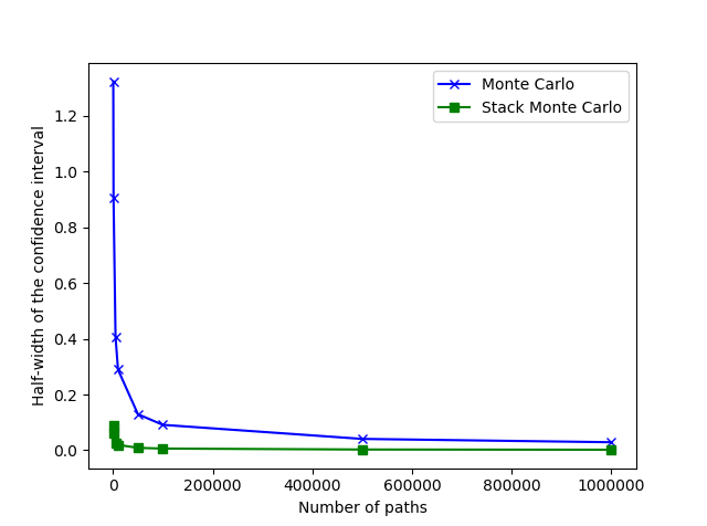
(a) Size of the confidence interval

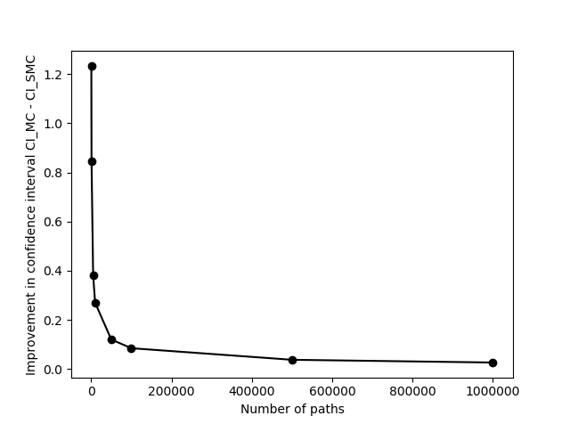
(b) Absolute confidence interval reduction

Figure 1. Variance reduction for a European Call option, between MC and StackMC.

The Monte Carlo variance is reduced as expected at a rate of $\mathcal{O}\left(N^{-1/2}\right)$, and the StackMC variance is consistently lower (Figure 1). The improvement brought by the stacking procedure decreases as the number of simulations increases, and is much more stable. In Figure 2, we observe a very modest improvement when increasing the number of folds. The computational expense increased with the number of folds, due in most part to the time spent fitting all the functions $g_{k}$. The random sub-sampling performs worse than K-folds in all cases, and performance depends of the balance between data used to estimate the model parameters (in-sample data), and to calculate $\alpha$ (out-of-sample data). Runtime is lower than that of K-folds, and decreases as the proportion of training data increased, largely due to the shorter time spent estimating $\alpha$ on a smaller test set.

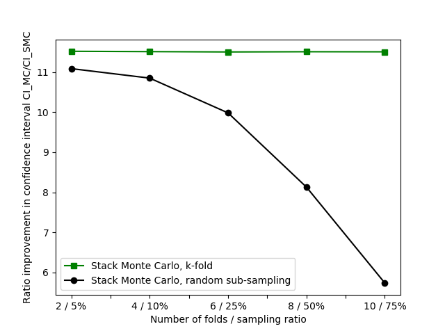
(a) Confidence interval reduction ratio

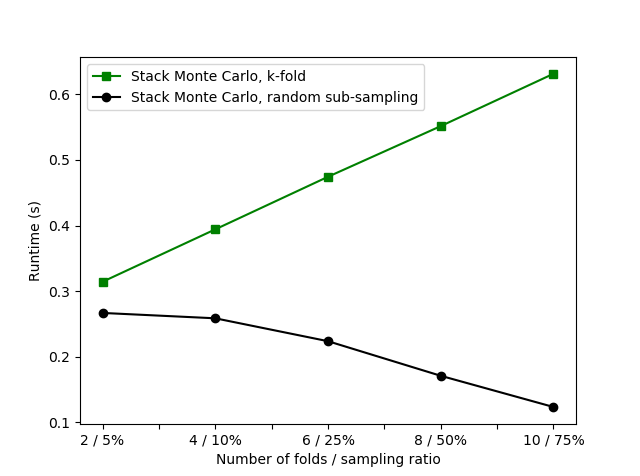
(b) Computation time of the stacking procedure

Figure 2. Variance reduction by cross-validation between $K$-folds and random sub-sampling.

3.2.1. Choice of fit model

To investigate the effect of the fit model, we perform the stacking procedure using polynomial functions $g(\cdot)$ of increasing order, and compare these results with those obtained for a piecewise linear fitting function (Figure 3). Rather than performing a non-linear fit to determine the inflection point, the piecewise function is obtained by filtering the zero-valued training data, and by estimating a linear fit to the remaining points. Values to the left of the intercept with the horizontal axis are then set to zero.

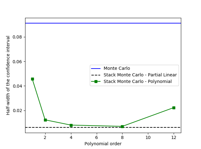
(a) Size of the confidence interval

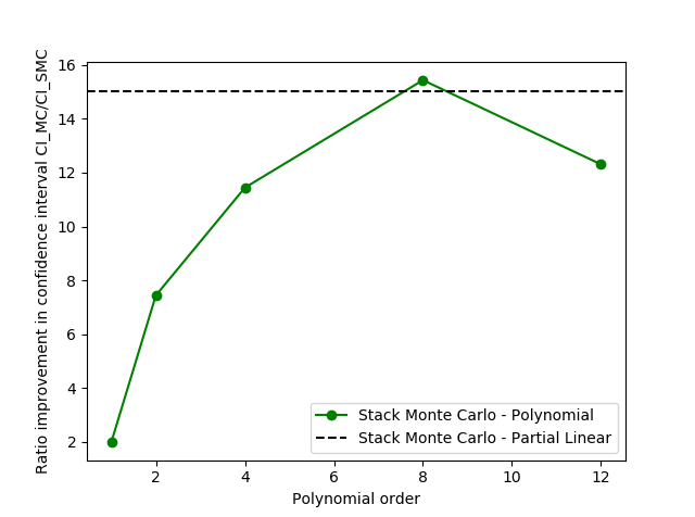
(b) Confidence interval reduction ratio

Figure 3. Variance reduction between MC and StackMC by fit model for a European Call option.

We observe a large improvement between orders $1$ and $2$, and small improvements thereafter up to order $8$, after which the results worsen (Figure 3). On average, the performance of the piecewise linear fitter is comparable to that of the polynomial functions (Figure 3). It is worth noting that our method for finding the piecewise linear function described above was chosen for computational speed. For comparison purposes, we also applied a non-linear method (using Scikit-learn) to fit a generic piecewise-linear function with one inflection point, and found the gains in variance reduction to be almost identical, albeit with a much higher computational cost.

3.3. Pricing Asian options

We are now interested in testing the Stacked Monte Carlo procedure on some path-dependent option, and we consider the case of an arithmetic Asian option, whose payoff is given by

$$\Phi_{T}:=\left(\frac{1}{M}\sum_{i=1}^{M}S_{t_{i}}-K\right)_{+},$$

for some strike $K$ and some monitoring dates $0<t_{1}<\ldots<t_{M}$. Under no-arbitrage arguments, the price of the Asian option reads, at time zero, $\mathrm{e}^{-rT}\mathbb{E}\left[\Phi_{T}\right]$. In the Black-Scholes model (10), by independence of the Gaussian increments, we can write (with $t_{0}=0$)

$$\sum_{i=1}^{M}S_{t_{i}}=S_{t_{0}}\sum_{i=0}^{M-1}\prod_{j=0}^{i}\frac{S_{t_{j+1}}}{S_{t_{j}}}=S_{0}\sum_{i=0}^{M-1}\prod_{j=0}^{i}\exp\left\{\left(r-\frac{\sigma^{2}}{2}\right)(t_{j+1}-t_{j})+\sigma\sqrt{t_{j+1}-t_{j}}X_{j}\right\}=:f(X_{1},\ldots,X_{M}),$$

where $(X_{1},\ldots,X_{M})$ is a centered Gaussian vector with identity covariance matrix. The fitting problem is thus of dimension $M$, where the variables $X_{1},\ldots,X_{M}$ correspond to the Brownian increments. With the same parameters as in Section 3.1, Figure 4 shows the results of the StackMC procedure using polynomial surfaces of degrees $2$ and $4$, and a piecewise linear surface as in Section 3.2.1.

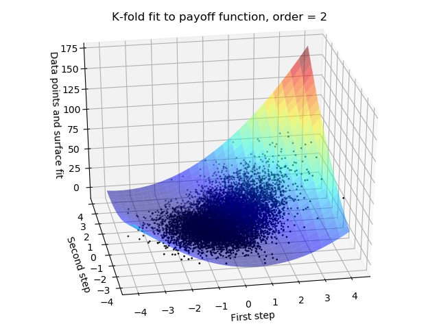
(a) Polynomial of order 2.

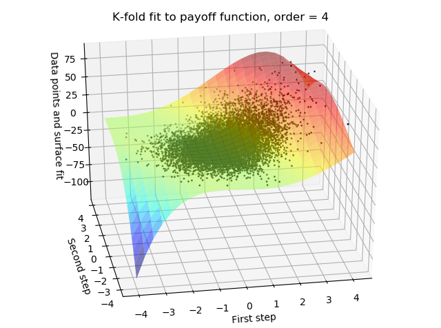
(b) Polynomial of order 4.

(c) Piecewise linear

Figure 4. StackMC variance reduction on an Asian option with $M=2$.

Tables 3, 4 and 5 illustrate the method with respectively $M=2$, $M=50$ and $M=100$, in order to to illustrate the effect of the dimensionality. In this example, the advantage of using a piecewise linear fitter is apparent: not only does this scheme deliver a greater improvement in the variance, but the computational effort required is such that it enables scaling of the problem to high dimensions. This property is essential to the application of the StackMC methodology to Asian options, for which each path is defined by an $M$-dimensional vector of Brownian increments. The runtime and memory requirements increase greatly when the number of time steps increases, and the performance of the second-order polynomial fit is consistently worse than that of the piecewise linear function.

					Improvement	Time
	Fit model	Price	CI	Runtime	Ratio	Total	Equivalent
MC		8.1024	0.0698	21.36
	Polynomial 2	8.1108	0.0097	1.23	7.18	22.59	1100.43
StackMC	Polynomial 4	8.1112	0.0064	1.54	10.97	22.90	2570.85
	Piecewise Linear	8.1117	0.0042	1.27	16.71	22.63	5963.16

Table 3. Comparison of MC and StackMC for the Asian option with $M=2$.

					Improvement	Time
	Fit model	Price	CI	Runtime	Ratio	Total	Equivalent
MC		5.8532	0.0502	22.24
StackMC	Polynomial 2	5.8582	0.0073	102.64	6.87	124.88	1049.08
	Piecewise Linear	5.8567	0.0502	3.10	19.88	25.34	8785.44

Table 4. Comparison of MC and StackMC for Asian option pricing with $M=50$ (the memory requirements for the 4th-order surface fit is prohibitive, and hence omitted).

					Improvement	Time
	Fit model	Price	CI	Runtime	Ratio	Total	Equivalent
MC		5.8209	0.0499	23.10
StackMC	Polynomial 2	5.8100	0.0076	1149.01	6.60	1172.12	1005.32
	Piecewise Linear	5.8102	0.0025	5.59	19.84	28.69	9092.11

Table 5. Comparison of MC and StackMC for Asian option pricing with $M=100$.

We add one final numerical example (Table 6) for the Asian case, in line with market considerations, namely with a piecewise linear model and daily time intervals ($M=365$ and $T=1$ year).

	Monte Carlo			Stacked Monte Carlo			Improvement		Time
Paths	Price	CI	Time	Price	CI	Time	Abs	Ratio	Total	Equivalent
1E4	5.7867	0.1570	2.97	5.7759	0.0084	2.10	0.0149	18.77	5.07	1045.88
1E5	5.7727	0.0496	29.56	5.7762	0.0025	18.12	0.0471	19.84	47.68	11635.73
1E6	5.7755	0.0157	299.46	5.7759	0.0008	199.37	0.0149	19.92	498.83	118783.86

Table 6. Comparison of MC and StackMC for Asian option pricing with $M=365$.

For $N=10^{5}$ Monte Carlo simulations, the additional time spent on the stacking procedure is about $18$ in our time units (equivalent to about ten seconds), which yields a nearly 20-fold improvement in the variance.

4. Stacked Monte Carlo for stochastic volatility models

We now adapt the Stacked Monte Carlo method to European and Asian options in local stochastic volatility models of the form

(11) $$\left\{\begin{array}[]{rll}\displaystyle\frac{\mathrm{d}S_{t}}{S_{t}}&=\displaystyle r\mathrm{d}t+\sigma_{\mathrm{loc}}(S_{t})\xi(t,V_{t})\mathrm{d}W_{t},&S_{0}>0,\\ \mathrm{d}V_{t}&=\displaystyle b(t,V_{t})\mathrm{d}t+a(t,V_{t})\mathrm{d}B_{t},&V_{0}>0,\end{array}\right.$$

where $r$ denotes the risk-free interest rate, and $W,B$ are two Brownian motions with correlation $\varrho\in[-1,1]$. The coefficients $b(\cdot)$, $a(\cdot)$, $\sigma_{\mathrm{loc}}(\cdot)$ and $\xi(\cdot)$ are left undefined, and are such that a unique solution to the system exists. Sets of sufficient conditions are classical, and can be found in [26, Chapter 5] for example.

4.1. Methodology

We start by discretising the system (11) following some Euler scheme. For the purpose of our methodology, any convergent schemes suffices, and an overview of such discretisations can be found in [28]. In particular, we start by drawing two matrices of standard Gaussian samples $\boldsymbol{W}\in\mathcal{M}_{N,M}$ and $\boldsymbol{B}\in\mathcal{M}_{N,M}$ (corresponding to the standardised Brownian increments of the stock price and the variance respectively), such that the correlation between $\boldsymbol{W}_{ij}$ and  $\boldsymbol{B}_{ij}$ is equal to $\rho$, for any $i=1,\ldots,N$ and $j=1,\ldots,M$, where $N$ and $M$ respectively denote the number of paths and the number of time steps. For each path, we can then compute the price of the option under consideration; we shall denote by $\boldsymbol{\Pi}=(\Pi_{1},\ldots,\Pi_{N})$ the corresponding vector of prices. Dividing the sample into $K$ folds of sizes $N_{1},\ldots,N_{K}$, we denote by $\boldsymbol{\Pi}^{k}\in\mathbb{R}^{N_{k}}$ the part of the vector $\boldsymbol{\Pi}$ corresponding to the $k$-th fold and by $\boldsymbol{\breve{\Pi}}^{k}\in\mathbb{R}^{N-N_{k}}$ the vector $\boldsymbol{\Pi}$ without $\boldsymbol{\Pi}^{k}$ ($k=1,\ldots,K$), and similarly for $\boldsymbol{W}^{k}\in\mathcal{M}_{N_{k},M}$ and $\breve{\boldsymbol{W}}^{k}\in\mathcal{M}_{N-N_{k},M}$ (column-wise). Up to reordering, we assume that the elements of $\boldsymbol{\Pi}$ and the rows of $\boldsymbol{W}$ are ordered, so that the first $N_{1}$ of them correspond to the first fold, and so on. For any $k=1,\ldots,K$, a predictor $\overline{\boldsymbol{\Pi}}^{k}$ of $\boldsymbol{\Pi}^{k}$ is then obtained as

$$\overline{\boldsymbol{\Pi}}^{k}\left(\boldsymbol{W}^{k}\right):=\mathcal{P}\left(\boldsymbol{W}^{k}\right),$$

where $\mathcal{P}$ denotes a polynomial of any order, the coefficients of which are calibrated through the fit of $\breve{\boldsymbol{\Pi}}^{k}$ on the cloud of points $\breve{\boldsymbol{W}}^{k}$. Note again that we do not use the $k$-th fold for the regression, but only for prediction (the in-sample data). This fit is essentially a supervised machine learning problem that can be solved either by least-square regressions or other techniques such as neural networks or random forests [20]. In order to set up the control variate, for each fold $k$, we compute the integral

(12) $$\widehat{\boldsymbol{\Pi}}^{k}:=\int\overline{\boldsymbol{\Pi}}^{k}\left(\boldsymbol{W}^{k}\right)n(\boldsymbol{W}^{k})\mathrm{d}\boldsymbol{W}^{k}=\int\mathcal{P}\left(\boldsymbol{W}^{k}\right)n(\boldsymbol{W}^{k})\mathrm{d}\boldsymbol{W}^{k},$$

and the version of the control variate (6) in the present context reads

$$\widetilde{\boldsymbol{\Pi}}^{k}:=\frac{1}{N_{k}}\sum_{j=1}^{N_{k}}\boldsymbol{\Pi}^{k}_{j}+\alpha\left(\widehat{\boldsymbol{\Pi}}^{k}-\frac{1}{N_{k}}\sum_{j=1}^{N_{k}}\overline{\boldsymbol{\Pi}}^{k}\left(\boldsymbol{W}^{k}_{j}\right)\right)$$

With our notations, we have $\boldsymbol{\Pi}^{k}_{j}=\boldsymbol{\Pi}_{N_{1}+\cdots+N_{k-1}+j}$; the final stacked estimator corresponding to (7) is then

$$\widetilde{\boldsymbol{\Pi}}_{\text{SMC}}:=\frac{1}{K}\sum_{k=1}^{K}\widetilde{\boldsymbol{\Pi}}^{k}.$$

On the numerical side, the computation of (12) may not be that straightforward. However, in the spirit of Remark 2.2, we restrict the integration domain to $\left\{\boldsymbol{W}^{k}:\mathcal{P}\left(\boldsymbol{W}^{k}\right)\geq 0\right\}$, which is natural as the payoff should remain positive for usual type of options such as Calls and Puts (other constraints can be considered should one be interested in other types of payoff functions). The linearity of $\mathcal{P}$ as well as this truncation domain thus yield the closed-form expressions from Remark 2.2 for the integral (12).

Remark 4.1.

In (11), we could replace the Brownian motion $B$ by a more general continuous Gaussian process $G$ such as a fractional Brownian motion or a Gaussian Volterra process, in the spirit of the recent rough volatility wave [5, 9, 12, 14, 22]. Since any continuous Gaussian Volterra process $G$ has a representation of the form $G_{t}=\int_{0}^{t}K(s,t)\mathrm{d}B_{s}$, for some Brownian motion $B$ defined on the same filtration as $G$ and some kernel $K(\cdot)$, then the knowledge of the increments $\boldsymbol{B}$ of $B$ provides the increments of $G$, and the Stacked Monte Carlo methodology above still applies.

4.2. Application to the Heston model

In order to motivate our results numerically, we specialise (11) to the Heston [21] model, under which the stock price satisfies the system

(13) $$\left\{\begin{array}[]{rll}\displaystyle\frac{\mathrm{d}S_{t}}{S_{t}}&=\displaystyle r\mathrm{d}t+\sqrt{V_{t}}\mathrm{d}W_{t},&S_{0}>0,\\ \mathrm{d}V_{t}&=\displaystyle\kappa(\theta-V_{t})\mathrm{d}t+\xi\sqrt{V_{t}}\mathrm{d}B_{t},&V_{0}>0,\end{array}\right.$$

for some parameters $\kappa,\theta,\xi>0$, where $W$ and $B$ are two Brownian motions with correlation $\varrho\in[-1,1]$. Several Euler schemes exist in the literature for the Heston model, in particular keeping track of the necessary positivity of the variance process, and we refer the interested reader to [1, 2, 3] for an overview. We consider the following set of parameters:

$$(S,K,r,T,V_{0},\kappa,\theta,\xi,\varrho)=(100,100,3.19,1,1.02,6.21,1.9,0.61,-0.7),$$

for which the reference price for of the European Call option, as reported in [8], is equal to $6.8061$. Table 7 and Table 8 show the results of the procedure with $M=365$ time steps. The results are not as clear as before, and only lead to a modest improvement in the variance.

	Monte Carlo			Stacked Monte Carlo			Improvement		Time
Nb Simulations	Price	CI	Time	Price	CI	Time	Abs	Ratio	Total	Equivalent
1E4	6.7930	0.1454	58.22	6.8158	0.0905	2.13	0.0549	1.61	60.35	150.20
5E4	6.8197	0.0652	290.58	6.8113	0.0388	8.70	0.0263	1.68	299.29	818.58
1E6	6.8118	0.0460	600.01	6.8088	0.0272	18.33	0.0188	1.69	618.34	1712.07

Table 7. StackMC for a European option in the Heston model.

	Monte Carlo			Stacked Monte Carlo			Improvement		Time
Nb Simulations	Price	CI	Time	Price	CI	Time	Abs	Ratio	Total	Equivalent
1E4	3.6115	0.0762	59.28	3.6150	0.0469	2.09	0.0293	1.62	61.37	156.46
5E4	3.6222	0.0342	304.00	3.6182	0.0200	7.93	0.0142	1.71	311.92	887.88
1E5	3.6159	0.0241	611.52	3.6173	0.0140	18.63	0.0101	1.72	630.14	1809.95

Table 8. StackMC for an Asian option in the Heston model.

An example of the agreement between the payoff function and the control variate is displayed in Figure 5. We note that the correlation is much higher in the case of constant volatility. Further, when a piecewise linear fit is achieved by filtering the non-zero data and fitting a linear function to the remainder, the fit appears biased toward smaller estimates (Figure 5(b)). This is because in the presence of the variance-produced ‘noise’, there are data points drawn for negative $\boldsymbol{x}$-values with a (small) positive payoff, which are not being filtered, biasing the fit to the left. This effect could be mitigated by fitting a piecewise linear function to the full dataset using a non-linear method (Figure 5(c)). Similarly, a larger variance reduction might be obtained by fitting a generic function, such as an $n^{\text{th}}$ order polynomial. However we are restricted by computational constraints to considering simple linear functions.

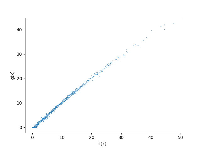
(a) Constant volatility.

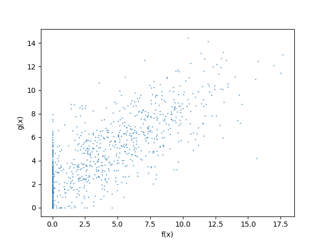
(b) Stochastic volatility.

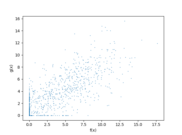
(c) Stochastic volatility.

Figure 5. Correlation between the data $f$ and the control variate $g$ for Asian options; (a) and (b) are obtained by filtering non-zero data and performing a linear fit, while (c) is determined by fitting a piecewise linear function to all the data using a non linear method.

4.3. Comparison with other variance reduction methods

We finally compare the results achieved using StackMC with those obtained with other commonly employed variance reduction methods. We concentrate on European and Asian Call options in the Black-Scholes model (10) as in Section 3.1 In all cases we draw $100,000$ simulations, apply K-fold cross validation with $K=2$, and choose a piecewise linear control variate function (fitted with a linear method to the positive data).

4.3.1. Antithetic updates

We compare StackMC to a standard Monte Carlo method with antithetic updates [18]. With the same values as in Section 3.1, From the results in Table 9, we see that StackMC achieves much greater variance reduction, for both European and Asian options.

	European option				Asian option
	Result		Improvement		Result		Improvement
	Price	CI	Abs	Ratio	Price	CI	Abs	Ratio
MC	10.450	0.0914
Antithetic MC	10.452	0.0646	0.0268	1.41	5.7803	0.0351	0.0145	1.41
StackMC	10.452	0.0061	0.0852	14.90	5.7763	0.0025	0.0471	19.75

Table 9. StackMC with antithetic updates.

4.3.2. Geometric mean control variate

For an arithmetic Asian option in the Black-Scholes models, it is common practice to use the geometric version as a control variate [25, 27], so that the original pricing problem is replaced with

(14) $$\widehat{C}_{\text{A}}:=\left(C_{\text{A}}-C_{\text{G}}\right)+\widehat{C}_{\text{G}},$$

with $C_{\text{A}}$ and $C_{\text{G}}$ the arithmetic and Geometric Call option prices. The difference $(C_{\text{A}}-C_{\text{G}})$ is computed using the Monte Carlo simulations. Note that $C_{\text{G}}$ is available in closed form, and is equal to [27]

$$C_{\text{G}}=\mathrm{e}^{-rT}\left[S_{0}\mathrm{e}^{aT}\mathcal{N}(d_{+})-K\mathcal{N}(d_{-})\right],$$

with

$$d_{\pm}:=\frac{\log(S_{0}/K)+\left(a\pm\frac{\sigma^{2}}{3}\right)T}{\sigma\sqrt{T}/3}\qquad\text{and}\qquad a:=\frac{1}{2}\left(r-\frac{\sigma^{2}}{2}\right).$$

The comparison between StackMC and the geometric mean as control variate for an Asian option with parameters as in Section 3.1 and $M=365$ is shown in Table 10.

	Result		Improvement
	Price	CI	Abs	Ratio
MC	5.7811	0.0050
CV MC	5.7795	0.0023	0.0473	21.71
StackMC	5.7758	0.0025	0.0470	19.82

Table 10. Comparison of StackMC and MC with Geometric control variate.

The variance reduction achieved with the geometric mean is slightly larger than that of StackMC. However, we may also apply Stacked MC to the new control variate problem (14) and compound the improvements. The results of the StackMC applied to the modified problem (14) are summarised in Table 11.

	Result		Improvement
	Price	CI	Abs	Ratio
StackMC+CV	5.7796	0.0011	0.0485	46.12

Table 11. StackMC on the modified problem.

The advantage of the stacking method is that whilst using the geometric mean is only successful in the particular case of the arithmetic Asian option, StackMC has general validity and can be applied (in theory) to any problem. As such, it applies to the control variate modified problem (14), which delivers an additional compounded variance reduction (Figure 6).

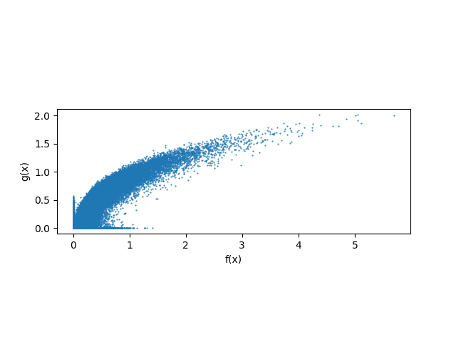
Figure 6. Correlation between the data and the fit function for the modified Asian option pricing problem using the Geometric mean as control variate.

References

- [1] A. Alfonsi. On the discretization schemes for the CIR (and Bessel squared) processes. Monte Carlo Methods and Applications, 11(4): 355-467, 2005.
- [2] A. Alfonsi. High order discretization schemes for the CIR process: Application to affine term structure and Heston models. Mathematics of Computation, 79: 209-237, 2010.
- [3] A. Alfonsi. Strong order one convergence of a drift implicit Euler scheme: Application to the CIR process. Statistics & Probability Letters, 83(2): 602-607, 2013.
- [4] J. Alonso, B. Tracey and D. Wolpert. Using supervised learning to improve Monte Carlo integral estimation. AIAA Journal, 51(8): 2015-2023, 2013.
- [5] C. Bayer, P. Friz and J. Gatheral. Pricing under rough volatility. Quantitative Finance, 16(6): 887-904, 2016.
- [6] C. Bayer and B. Stemper. Deep calibration of rough stochastic volatility models. arXiv:1810.03399, 2018.
- [7] F. Black and M. Scholes. The pricing of options and corporate liabilities. Journal of Political Economy, 81(3): 637-654, 1973.
- [8] M. Broadie and O. Kaya. Exact simulation of stochastic volatility and other affine jump diffusion processes. Operations Research, 54(2): p. 217-231, 2006.
- [9] F. Comte and E. Renault. Affine fractional stochastic volatility models. Annals of Finance, 8(2–3): 337-378, 2012.
- [10] J. De Spiegeleer, D. Madan, S. Reyners and W. Schoutens. Machine learning for quantitative finance: Fast derivative pricing, hedging and fitting. SSRN:3191050, 2018.
- [11] G. Dimitroff, D. Röder and C. Fries. Volatility model calibration with convolutional neural networks. SSRN:3252432, 2018.
- [12] O. El Euch and M. Rosenbaum. The characteristic function of rough Heston models. Math. Finance, 29(1): 3-38, 2019.
- [13] R. Ferguson and A. Green. Deeply learning derivatives. arXiv:1809.02233, 2018.
- [14] J. Gatheral, T. Jaisson and M. Rosenbaum. Volatility is rough. Quantitative Finance, 18(6): 933-949, 2018.
- [15] M.B. Giles. Multilevel Monte Carlo Path simulation. Operations Research, 56(3): 607-617, 2008.
- [16] M.B. Giles. Multilevel Monte Carlo methods. Acta Numerica, 24: 259-328, 2015.
- [17] M.B. Giles and L. Szpruch. Multilevel Monte Carlo methods for applications in finance. Recent Advances in Computational Finance (Edited by Gerstner, Kloeden), World Scientific, 2013.
- [18] P. Glasserman. Monte Carlo methods in Financial Engineering. Springer-Verlag, 2003.
- [19] J.T. Hahn Option pricing using artificial neural networks: an Australian perspective. PhD thesis, Bond University, 2013.
- [20] T. Hastie, R. Tibshirani and J. Friedman. The elements of statistical learning: data mining, inference, and prediction. Springer, Second Edition, 2009.
- [21] S. Heston. A closed-form solution for options with stochastic volatility with applications to bond and currency options. The Review of Financial Studies, 6(2): 327-343, 1993.
- [22] B. Horvath, A. Jacquier and P. Tankov. Volatility options in rough volatility models arXiv:1802.01641, 2019.
- [23] B. Horvath, A. Muguruza and M. Tomas. Deep learning volatility. arXiv:1901.09647, 2019.
- [24] J.M. Hutchinson, A. Lo and T. Poggio. A nonparametric approach to pricing and hedging derivative securities via learning networks. Journal of Finance, 49(3): 851-889, 1994.
- [25] M.S. Joshi. Graphical Asian options. Wilmott Journal, 2(2): 97-107, 2010.
- [26] I. Karatzas and S. Shreve. Brownian Motion and Stochastic Calculus. Springer, 8th Edition, 1991.
- [27] A. Kemna and A. Vorst. A pricing method for options based on average asset values. Journal of Banking and Finance, 14(1): 113-129, 1990.
- [28] P. Kloeden and E. Platen. Numerical solution of stochastic differential equations. Springer-Verlag Berlin Heidelberg, 1992.
- [29] A. Kondratyev. Learning curve dynamics with artificial neural networks. Risk Magazine, May 2018.
- [30] W. A. McGhee. An artificial neural network representation of the SABR stochastic volatility model. SSRN:3288882, 2018.
- [31] J. Sharples and J. Pezzey. Expectations of linear functions with respect to truncated multinormal distributions. Environmental Modelling & Software, 22(7): 915-923, 2007.
- [32] H. Stone. Calibrating rough volatility models: a convolutional neural network approach. arXiv:1812.05315, 2018.
- [33] B. Tracey and D. Wolpert. Reducing the error of Monte Carlo Algorithms by learning control variates. 29th Conference on Neural Information Processing Systems, Barcelona, 2016.