Color flux tubes in $SU(3)$ Yang-Mills theory:
an investigation with the connected correlator

Abstract

In this work we perform an investigation of the flux tube between two static color sources in four dimensional $SU(3)$ Yang-Mills theory, using the so called connected correlator. Contrary to most previous studies we do not use any smoothing algorithm to facilitate the evaluation of the correlator, that is performed using only stochastically exact techniques. We first examine the renormalization properties of the connected operator, then we present our numerical data for the longitudinal chromoelectric component of the flux tube, that are used to extract the dual superconductivity parameters.

I Introduction

The investigation of the color flux tubes connecting static sources in non-abelian gauge theories has become a standard tool to study color confinement Fukugita:1983du ; Flower:1985gs ; Wosiek:1987kx ; Sommer:1987uz ; DiGiacomo:1989yp ; DiGiacomo:1990hc ; Bali:1994de ; Haymaker:1994fm ; Cea:1995zt ; Okiharu:2003vt ; Bissey:2006bz ; Bicudo:2011hk ; Bakry:2014gea . Indeed, in lattice simulations, color sources are seen to be connected by tube-like structures for all the values of the coupling constant (at zero temperature). This is a strong indication that the mechanism responsible for color confinement is the same at weak and at strong coupling, in which limit color flux tubes naturally emerge Kogut:1974ag , and the area-law of the Wilson loops can be analytically proven Osterwalder:1977pc .

To study flux tubes on the lattice we need an observable whose average value will provide us information about the flux tube details: more specifically the value of this observable has to be related to that of the field strength in the background of a couple of static color sources. A quantity that satisfies this requirement can be built by using the correlator of a Polyakov loops pair with a plaquette: the pair of Polyakov loops represents a couple of static color charges (a Wilson loop is also often used for this purpose) while the plaquette probes the field strength in the background of the static charges.

This general idea is common to all numerical implementations, however in the literature two different ways of defining the basic correlator are present: the first possibility is to use the expression Fukugita:1983du

$$\rho_{disc}=\frac{\langle\mathrm{Tr}(P_{\boldsymbol{r}})\mathrm{Tr}(P_{\boldsymbol{r}^{\prime}}^{{\dagger}})\mathrm{Tr}(U_{p})\rangle}{\langle\mathrm{Tr}(P_{\boldsymbol{r}})\mathrm{Tr}(P_{\boldsymbol{r}^{\prime}}^{{\dagger}}))\rangle}-\langle\mathrm{Tr}(U_{p})\rangle\ ,$$ (1)

where $P_{\boldsymbol{r}}$ stands for the Polyakov loop at spatial position $\boldsymbol{r}$ and $U_{p}$ for the plaquette operator; this is known as the “disconnected” correlator. Another possibility is to use the definition DiGiacomo:1989yp ; DiGiacomo:1990hc

$$\begin{gathered}\rho_{conn}=\frac{\langle\mathrm{Tr}(P_{\boldsymbol{r}}LU_{p}L^{{\dagger}})\mathrm{Tr}(P_{\boldsymbol{r}^{\prime}}^{{\dagger}})\rangle}{\langle\mathrm{Tr}(P_{\boldsymbol{r}})\mathrm{Tr}(P_{\boldsymbol{r}^{\prime}}^{{\dagger}})\rangle}-\\ -\frac{1}{N_{c}}\frac{\langle\mathrm{Tr}(P_{\boldsymbol{r}})\mathrm{Tr}(P_{\boldsymbol{r}^{\prime}}^{{\dagger}})\mathrm{Tr}(U_{p})\rangle}{\langle\mathrm{Tr}(P_{\boldsymbol{r}})\mathrm{Tr}(P_{\boldsymbol{r}^{\prime}}^{{\dagger}})\rangle}\ ,\end{gathered}$$ (2)

where $N_{c}$ is the number of colors and $L$ is the parallel transporter associated to the path shown in Fig. 1; $\rho_{conn}$ is known as the “connected” correlator and $L$ is often called the “Schwinger line” in the literature. Both $\rho_{disc}$ and $\rho_{conn}$ are related to color flux tubes but they are not equivalent; in fact they are associated to different physical observables. This can be readily understood by looking at their naive continuum limit, in which the plaquette operator $U_{p}$ is expanded in powers of the lattice spacing $a$: $\rho_{disc}$ scales to the continuum as $a^{4}$ and gives access to $\mathrm{Tr}(F_{\mu\nu}^{2})$ (we are assuming $U_{p}$ oriented in the $\mu\nu$ plane), $\rho_{conn}$ scales to the continuum as $a^{2}$ and it is linear in $F_{\mu\nu}$ (see e.g. DiGiacomo:1989yp ; DiGiacomo:1990hc for more details).

Figure 1: Graphical representation of the numerator of the first term of Eq. (2). Ellipses denote the Polyakov loops (at distance $d$ from each other) and the string $L$ connects one Polyakov loop with the plaquette, first reaching the midpoint between the Polyakov loops at $d/2$, then moving in the transverse direction for a distance $d_{t}$. The plaquette is drawn parallel to the plane identified by the two Polyakov loops since this is the case that will be studied in this paper, but its orientation can a priori be generic.

Since $\rho_{disc}$ and $\rho_{conn}$ do not provide equivalent physical information, the choice of the operator to be used requires some discussion. Two arguments that have been adopted in the past to advocate the use of one operator or the other are the following: on one hand the operator $\rho_{disc}$ is theoretically better understood, since it can be easily shown to be multiplicatively renormalizable (see the discussion in Sec. II), and the renormalization constant needed to cancel logarithmic divergences can be fixed by using a lattice sum rule (see e.g. Bali:1994de ). On the other hand $\rho_{disc}$ is noisier than $\rho_{conn}$, and noise reduction was the original motivation for the introduction of the connected correlator in DiGiacomo:1989yp ; DiGiacomo:1990hc : since $\rho_{disc}$ probes the square of the field-strength it is more sensitive to ultraviolet (UV) fluctuations.

The choice of the operator to be used was thus largely based on the importance attributed to fluctuations. Sometimes UV fluctuations have a prominent role in the physical phenomenon to be studied, a prototypical example being the fluctuation-induced broadening of flux tubes Luscher:1980iy . In these cases the choice of the disconnected operator is mandatory, and specific stochastically exact noise-reduction techniques have been typically adopted to measure it Allais:2008bk ; Gliozzi:2010zv ; Gliozzi:2010jh ; Cardoso:2013lla ; Amado:2013rja ; Caselle:2016mqu .

When fluctuations were not expected to be important for the physical problem studied, the operator $\rho_{conn}$ has been the most common choice Cardaci:2010tb ; Cea:2012qw ; Cea:2014uja ; Cea:2015wjd ; Baker:2018mhw , supplemented by the use of smoothing algorithms to reduce UV noise. In studies performed with dynamical fermions only $\rho_{conn}$ has been used so far Cea:2017ocq ; Bonati:2018uwh , since the accessible statistics are much lower than in the pure glue case, and stochastically exact error reduction techniques (see Ce:2016ajy ) are not easily applicable and still not widely used.

An important point to be noted is that smoothing has always been used to reduce the effect of UV fluctuations in $\rho_{conn}$, however this standard procedure can a priori also induce systematical errors in the flux tube measure. Indeed in Bonati:2018uwh a worrisome dependence of the physical results on the amount of smoothing adopted was noted (see also Cea:2012qw for the case of Yang-Mills theory).

The aim of this work is to study $\rho_{conn}$ without using any smoothing algorithm, in order to understand if the connected operator can be used in a coherent field-theoretical setup to extract physical quantities related to flux tubes. For this purpose we evaluate the connected correlator $\rho_{conn}$ in four dimensional $SU(3)$ Yang-Mills theory using only stochastically exact techniques (i.e. multihit Parisi:1983hm and multilevel Luscher:2001up algorithms). To physically interpret these data we need to study the renormalization of the connected correlator $\rho_{conn}$: in our data the singularities related to the continuum limit (that are usually hidden by the use of smoothing) are clearly visible and we need to take care of them. The renormalization of $\rho_{conn}$ is far less trivial than that of $\rho_{disc}$, however we will show that $\rho_{conn}$ renormalizes multiplicatively, and it can be used to extract physically relevant information.

The paper is organized as follows: in Sec. II we discuss the issues related to the renormalization of $\rho_{conn}$, using arguments largely based on Berwein:2012mw ; Berwein:2013xza , where the renormalization of cyclic Wilson loops was addressed. In Sec. III we introduce the numerical setup adopted, we present the results obtained for the longitudinal chromoelectric field, and we discuss the physical implications of these results for the dual superconductor model of the vacuum. Finally, in Sec. IV we draw our conclusions.

II Renormalization of $\rho_{conn}$

In order to discuss the renormalization of $\rho_{conn}$ it seems appropriate to start by briefly recalling some general facts about the renomalization of loop operators.

A loop operator is a generalized Wilson loop, which in the continuum can be written as

$$W_{C}=\mathrm{Tr}\left[\mathcal{P}\exp\left(i\oint_{C}A_{\mu}\mathrm{d}x^{\mu}\right)\right],$$ (3)

where $C$ is a closed curve and $\mathcal{P}$ stands for path-ordered. The systematic study of the divergences associated to these operators in four dimensional gauge theory was initiated in Polyakov:1980ca , where it was suggested that $W_{C}$ is multiplicatively renormalizable if $C$ is piecewise smooth and not self-intersecting. From a one loop computation with cut-off regularization two sources of divergences were identified in Polyakov:1980ca : logarithmic divergences originate from the points at which $C$ is not differentiable, while linear divergences are always present, they exponentiate and globally contribute with a term of the form $\exp(c\mathcal{L}(C)/a)$, where $\mathcal{L}(C)$ is the length of the curve, $a$ is the UV cut-off and $c$ is a constant.

If $C$ is smooth it was shown in Dotsenko:1979wb that $W_{C}$ is finite at all orders of perturbation theory, after the usual charge renormalization is performed. The case of a non-smooth curve was studied in Brandt:1981kf , where it was proven that to each cusp with angle $\gamma$ a multiplicative renormalization constant has to be associated, whose value depends just on $\gamma$. The case of self-intersecting curves was also studied in Brandt:1981kf : in this case operator mixing between operators corresponding to different color contractions at the crossing points has also to be taken into account. The final result is the following: if $r$ intersection points (corresponding to the sets of intersection angles $\{\theta_{1}\},\ldots,\{\theta_{r}\}$) and $s$ cusps (corresponding to the angles $\gamma_{1},\ldots,\gamma_{s}$) are present, then renormalization matrices and renormalization constants exist such that every color contraction $W_{C}^{i_{1},\ldots,i_{r}}$ can be renormalized by using

$$\left.W_{C}^{i_{1},\ldots,i_{r}}\right|_{R} =Z(\gamma_{1})\cdots Z(\gamma_{s})\times$$ (4)

$$\times Z_{i_{1}j_{1}}(\{\theta_{1}\})\cdots Z_{i_{r}j_{r}}(\{\theta_{r}\})W_{C}^{j_{1},\ldots,j_{r}}\ ,$$

where the exponentials associated to linear divergences are implied. In Brandt:1981kf the possibility for different color contractions to have different lengths was however not considered, and this could seem to be a source of problems for the renormalization of $\rho_{conn}$.

Let us start by studying the renormalization of $\rho_{conn}$ in a scheme in which no power-law divergences are present (like e.g. minimal subtraction), so that we can use Eq. (4) without worrying of the complications related to linear divergences. In this case Polyakov loops do not need any renormalization, since they are associated to smooth contours, and the denominator $\langle\mathrm{Tr}(P_{\boldsymbol{r}})\mathrm{Tr}(P_{\boldsymbol{r}^{\prime}}^{{\dagger}})\rangle$ of Eq. (2) is finite once charge renormalization is performed. For the same reason the term $\mathrm{Tr}(P_{\boldsymbol{r}^{\prime}}^{{\dagger}})$ in the numerator is also harmless and we can just concentrate on the term

$$O_{1}=\mathrm{Tr}\left(P_{\boldsymbol{r}}LU_{p}L^{{\dagger}}\right)\ .$$ (5)

The path associated to $O_{1}$ is not smooth at three point: the point at which $L$ and $L^{{\dagger}}$ connects to $P_{\boldsymbol{r}}$, the point at which they connects to $U_{p}$ and the corner point of $L$ and $L^{{\dagger}}$. All the rest of the contour contributes only to linear divergences, that we are neglecting for the moment.

In studying the renormalization of $O_{1}$ we have to take into account the mixing with all the operators that can be build from $O_{1}$ using different color contractions at the crossing points. Eight color contractions can be built (2 different contractions for each crossing point), however it is easy to realize, using $LL^{{\dagger}}=1$ and analogous relations, that all the contractions that are not equal to $O_{1}$ are equal to

$$O_{2}=\frac{1}{N_{c}}\mathrm{Tr}\left(P_{\boldsymbol{r}}\right)\mathrm{Tr}\left(U_{p}\right)\ ,$$ (6)

where the $1/N_{c}$ factor is needed to keep the same normalization of Eq. (5). From the previous general discussion it follows immediately that $O_{2}$ is multiplicatively renormalizable, a fact that will be used soon.

Eq. (4) implies that we have to consider in general an $8\times 8$ mixing matrix, which is the tensor product of the three basic $2\times 2$ mixing matrices, however very stringent constraints are imposed on this $8\times 8$ matrix by the fact that only two color contractions are different from each other, and by the fact that $O_{2}$ is multiplicatively renormalizable.

Let us discuss explicitly the case $d_{t}=0$ (see Fig. 1), in which we have just the tensor product of two $2\times 2$ mixing matrices and $4$ color contractions. Denoting the two $2\times 2$ mixing matrices by $Z^{A}$ and $Z^{B}$ we thus have

$$\left(\begin{array}[]{c}O_{1}^{(R)}\\ O_{2}^{(R)}\\ O_{2}^{(R)}\\ O_{2}^{(R)}\end{array}\right)=\left(\begin{array}[]{cc}Z^{A}_{00}Z^{B}&Z^{A}_{01}Z^{B}\\ Z^{A}_{10}Z^{B}&Z^{A}_{11}Z^{B}\end{array}\right)\left(\begin{array}[]{c}O_{1}\\ O_{2}\\ O_{2}\\ O_{2}\end{array}\right)\ ,$$ (7)

where the apex $(R)$ stands for “renormalized” and

$$Z^{B}=\left(\begin{array}[]{cc}Z^{B}_{00}&Z^{B}_{01}\\ Z^{B}_{10}&Z^{B}_{11}\end{array}\right)\ .$$ (8)

Since $O_{2}$ renormalizes multiplicatively, the coefficients $Z^{A}_{10}$ and $Z^{B}_{10}$ have to vanish, otherwise $O_{2}^{(R)}$ would depend also on $O_{1}$. If we use $Z^{A}_{10}=Z^{B}_{10}=0$ we see that the last three lines of Eq. (7) are consistent with each other only if

$$Z^{A}_{00}+Z^{A}_{01}=Z^{A}_{11}\ ,\quad Z^{B}_{00}+Z^{B}_{01}=Z^{A}_{11}\ .$$ (9)

It is then simple to verify that Eq. (7) collapses to

$$\left(\begin{array}[]{c}O_{1}^{(R)}\\ O_{2}^{(R)}\end{array}\right)=\left(\begin{array}[]{cc}Z_{1}&Z_{2}-Z_{1}\\ 0&Z_{2}\end{array}\right)\left(\begin{array}[]{c}O_{1}\\ O_{2}\end{array}\right)\ ,$$ (10)

where

$$Z_{1}=Z^{A}_{00}Z^{B}_{00}\ ,\quad Z_{2}=Z^{A}_{11}Z^{B}_{11}\ .$$ (11)

As a consequence we finally have

$$O_{1}^{(R)}-O_{2}^{(R)}=Z_{1}(O_{1}-O_{2})$$ (12)

which means that $\rho_{conn}$ renormalizes multiplicatively.

The same argument (which is an adaptation of the one used in Berwein:2012mw ) can be repeated without changes also when $d_{t}>0$, in which case we have to start from the tensor product of three $2\times 2$ mixing matrices. Since the renormalization constants only depend on the set of intersection angles, the value of $Z_{1}$ is the same for all the positive $d_{t}$ values, but it differs from the one at $d_{t}=0$, due to the presence of new logarithmic divergences for $d_{t}>0$.

Let us now consider a renormalization scheme in which linear divergences are present. The argument to show that $\rho_{conn}$ is multiplicatively renormalizable also in this case is exactly the same that was used for cyclic Wilson loops in Berwein:2013xza , to which we refer for further details and some enlightening examples. Here we will just briefly sketch some basic steps of the proof for the benefit of the reader and to fix the notation. The main ingredient that is needed is the relation between an operator acting in the fundamental representation of $SU(N_{c})$ (that we will denote by $U$) and the corresponding operator acting in the adjoint representation (that we will denote by $U^{\mathrm{adj}}$), which is

$$U^{\mathrm{adj}}_{ab}=2\mathrm{Tr}(U^{{\dagger}}T_{a}UT_{b})\ ,$$ (13)

where $T_{a}$ are the $SU(N_{c})$ generators, with the normalization $\mathrm{Tr}(T_{a}T_{b})=\frac{1}{2}\delta_{ab}$.

By writing $P_{\boldsymbol{r}}$ and $U_{p}$ in the base $\{1,T_{a}\}$ and using Eq. (13) it is simple to show that

$$O_{1}-O_{2} =\mathrm{Tr}(P_{\boldsymbol{r}}LU_{p}L^{{\dagger}})-\frac{1}{N_{c}}\mathrm{Tr}(U_{p})\mathrm{Tr}(P_{\boldsymbol{r}})=$$ (14)

$$=2\sum_{ab}\mathrm{Tr}(P_{\boldsymbol{r}}T_{a})L_{ab}^{\mathrm{adj}}\mathrm{Tr}(U_{p}T_{b})\ .$$

We thus see that $O_{1}-O_{2}$ can be written as a single generalized loop function in which traces in different representations are present: two traces in the fundamental representation (explicitly denoted by $\mathrm{Tr}$) and a trace in the adjoint representation (the summation on $a,b$).

This expression is particularly convenient since it was shown in Berwein:2013xza (using the exponentiation theorems of Gardi:2010rn ; Gardi:2013ita ) that linear divergences factorize also in untraced loop operators, and they can be cancelled by multiplicative factors of the form $\exp(-c_{r}\mathcal{L}(C_{r})/a)$, where $c_{r}$ is a representation dependent coefficient, $a$ is the UV cut-off, and $\mathcal{L}(C_{r})$ is the length in physical units of the curve $C_{r}$ associated to the representation $r$.

Applying this result to the operator $O_{1}-O_{2}$ we get

$$[O_{1}-O_{2}]^{(R)}=\exp\left[-\frac{c_{a}}{a}\left(\frac{d}{2}+d_{t}\right)\right]\times$$ (15)

$$\quad\times\exp\left[-\frac{c_{f}}{a}L_{t}-4c_{f}\right]Z_{1}[O_{1}-O_{2}]\ ,$$

where $c_{f}$ and $c_{a}$ are the constants associated to the fundamental and adjoint representations, $\frac{d}{2}+d_{t}$ is the length of the contour in the adjoint representation (see Fig. 1) and $L_{t}$ is the temporal extent of the lattice in physical units. $Z_{1}$ is the renormalization constant associated to logarithmic divergences that was previously introduced in Eq. (11), while the term $4c_{f}$ is associated to the plaquette, that has length $4a$, does not generate linear divergences in the continuum and can be safely neglected. Since a factor $e^{-c_{f}L_{t}/a}$ is associated to each Polyakov loop, we finally have

$$\rho_{conn}^{(R)}=\exp\left[-\frac{c_{a}}{a}\left(\frac{d}{2}+d_{t}\right)\right]Z_{1}(a,d_{t})\rho_{conn}\ ,$$ (16)

where $Z_{1}$ is independent of $d$ and assumes two different values for $d_{t}=0$ or $d_{t}\neq 0$.

III Numerical results

III.1 Setup

$N_{s}$	$\beta$	$a(\beta)$ [fm]	$d$	$n_{\mathrm{upd}}$
20	6.0	0.0931	4	200
28	6.2601	0.0621	6	1000
36	6.47466	0.0456	8	3000

Table 1: Simulation parameters: $N_{s}$ is the lattice extent in lattice units, $\beta$ is the bare coupling constant, $a(\beta)$ is the lattice spacing, $d$ the distance between the Polyakov loops in lattice units, and $n_{\mathrm{upd}}$ the number of internal updates of the multilevel algorithm.

As anticipated in the introduction, we study $\rho_{conn}$ in four dimensional $SU(3)$ Yang-Mills theory, discretized on the lattice by using the standard Wilson action Wilson:1974sk :

$$S=\sum_{p}\beta\left(1-\frac{1}{3}\mathrm{Re}\mathrm{Tr}U_{p}\right)\ .$$ (17)

The connected correlator defined in Eq. (2) can be estimated by using a combination of multihit Parisi:1983hm and multilevel Luscher:2001up techniques: multihit can be applied to the links of the Polyakov loops and to a single link of the plaquette. The multilevel method can be easily adapted to measure $\rho_{conn}$, since almost all the links entering $LU_{p}L^{{\dagger}}$ are associated to a single time slice of the lattice, with the only possible exception of three links entering $U_{p}$ (if the plaquette is a temporal one). The time slice identified by $L$ has been chosen to lay in the bulk of the corresponding slice of the multilevel algorithm, so that the links entering $L$ and $L^{{\dagger}}$ are updated in the multilevel. If a slice of thickness $\Delta=2a$ was used for the case of a temporal plaquette, the upper link of the plaquette would thus be fixed during the multilevel. However for all the cases studied in this work a single level of the multilevel algorithm was used, with slices of thickness $\Delta=4a$, so that all the links of $LU_{p}L^{{\dagger}}$ are updated. The number of internal updates of the multilevel algorithm was optimized by using a technique analogous to the one discussed in Luscher:2001up .

Simulations were performed on symmetric lattices ($N_{s}=N_{t}$), and in Tab. 1 we report the simulation details. The plaquette $U_{p}$ which appears in Eq. (2) was always chosen to be parallel to the plane identified by the two Polyakov loops, since we are interested in studying the longitudinal chromoelectric field, which in all previous studies was shown to be the dominant component of the flux tube.

The coupling values were chosen in such a way that $d=4a,6a$ and $8a$ correspond to the same distance in physical units; for this purpose the parametrization of $a(\beta)$ obtained in Necco:2001xg was used. Parameters in Tab. 1 fix the physical distance between the Polyakov loops to about $0.37\,\mathrm{fm}$ (using $r_{0}\simeq 0.5\,\mathrm{fm}$ for the Sommer scale Sommer:1993ce ), and the dimensionless lattice size was rescaled in order to have (almost) constant physical volume. Note that $d\simeq 0.37\,\mathrm{fm}$ is quite smaller than the typical values that have been used in recent works, which range from $0.54\,\mathrm{fm}$ to 0.$76\,\mathrm{fm}$ (see e.g. Cea:2014uja ; Cea:2015wjd ). Test simulations were also performed on the lattice $28^{4}$ with coupling $\beta=6.0$, which excluded the presence of sizable finite size effects in our data. Data points corresponding to different values of $d_{t}$ have been extracted from independent simulations, hence they are statistically independent from each other.

III.2 Results for the chromoelectric field

From the naive continuum limit of $\rho_{conn}$ in Eq. (2) we can define the longitudinal (due to our choice of the plaquette orientation, see Sec. III.1) chromoelectric field by using the expression

$$E_{L}(d,d_{t})=\frac{\sqrt{\beta/6}}{a^{2}(\beta)}\,\rho_{conn}(d,d_{t})\ ,$$ (18)

where in our simulations $d$ is fixed to about $0.37\,\mathrm{fm}$, and $d_{t}$ denotes the transverse distance from the center of the flux tube (see Fig. 1). From the discussion in Sec. II it follows that we can not expect $E_{L}$ defined in this way to have a nontrivial continuum limit. Indeed data shown in Fig. 2 indicate that $E_{L}(d,d_{t})$ converges to zero as the continuum limit is approached.

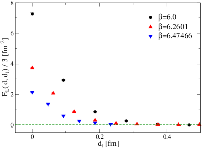
Figure 2: $E_{L}(d,d_{t})$ computed from Eq. (18) for three values of the coupling constant and $d\simeq 0.37\,\mathrm{fm}$.

To properly define the continuum limit of $E_{L}$ we have to use Eq. (16) and define

$$E_{L}^{(R)}(d,d_{t})=Z_{L}(d,d_{t},a)Z_{1}(a,d_{t})E_{L}(d,d_{t})\ ,$$ (19)

where $Z_{1}(a,d_{t})$ is the renormalization constant associated to logarithmic divergences (which is different for $d_{t}=0$ and $d_{t}\neq 0$), and we introduced the shorthand

$$Z_{L}(d,d_{t},a)=\exp\left[-\frac{c_{a}}{a}\left(\frac{d}{2}+d_{t}\right)\right]$$ (20)

to denote the multiplicative factor needed to remove linear divergences. To completely define $E_{L}^{R}$ we thus have to fix the three constants $c_{a}$ and $Z_{1}(a,d_{t})$ (for $d_{t}=0$ and $d_{t}\neq 0$).

The numerical value of $Z_{1}(a,d_{t})$ could be computed in perturbation theory, however some interesting physical observables can be studied also without a precise knowledge of this renormalization constant. This is due to the fact that, for $d_{t}>0$, $Z_{1}$ is a multiplicative factor independent of $d_{t}$, hence the functional form of $E_{L}^{(R)}(d,d_{t})$ for $d_{t}>0$ is completely fixed also without any knowledge of $Z_{1}$. However, also to study just the functional form of $E_{L}^{(R)}(d,d_{t})$, we need to fix $c_{a}$.

$N_{t}$	$N_{s}$	$\beta$
4	16	5.8
5	20	5.91225
6	24	6.01388
7	28	6.10767
8	32	6.19513
9	36	6.27708
10	40	6.35394

Table 2: Simulation points used to fix the value of the renormalization constant $c_{a}$

Since $c_{a}$ is a fundamental property of the discretization adopted, independent of the specific adjoint loop function used and of the infrared properties of the theory, we have the freedom of choosing the simplest numerical setup available to fix its value. We decided to extract if from the continuum scaling of the Polyakov loop in the adjoint representation at finite temperature, which is an observable that is easily computed to high precision.

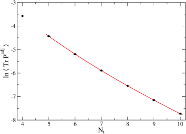
Figure 3: Continuum scaling of $\langle\mathrm{Tr}P^{\mathrm{adj}}\rangle$ in the high temperature phase. The continuous line is the result of a fit of the form $k_{0}+c_{a}N_{t}+k_{1}/N_{t}$.

For this purpose we performed simulations starting from a $4\times 16^{3}$ lattice at $\beta=5.8$ (the deconfinement transition on $N_{t}=4$ lattices takes place at $\beta_{c}=5.6925(2)$, see Fingberg:1992ju ), then increasing the value of $N_{t}$ keeping the physical temperature constant and the aspect ratio fixed to $4$, see Tab. 2. The average value of the Polyakov loop in the adjoint representation can be computed by using the relation

$$\mathrm{Tr}P^{\mathrm{adj}}=|\mathrm{Tr}P|^{2}-1\ ,$$ (21)

which is an easy consequence of Eq. (13), and from the discussion in Sec. II if follows that $\langle\mathrm{Tr}P^{\mathrm{adj}}\rangle$ scales to the continuum as $\exp(c_{a}N_{t})$.

Numerical results obtained for $\langle\mathrm{Tr}P^{\mathrm{adj}}\rangle$ are shown in Fig. 3, in which some deviations from the asymptotic $\exp(c_{a}N_{t})$ behaviour are also visible. To extract the value of $c_{a}$ fits of the form

$$\ln\langle P^{\mathrm{adj}}\rangle=k_{0}+c_{a}N_{t}+\frac{k_{1}}{N_{t}}+\frac{k_{2}}{N_{t}^{2}}$$ (22)

have been performed, and the stability of the fit under changes of the fit range and of the functional form adopted (i.e. by setting $k_{2}=0$) has been investigated. As our final estimate we report the value

$$c_{a}=-0.45(2)\ .$$ (23)

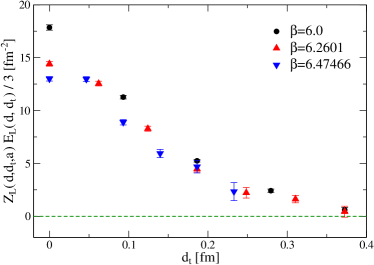
Figure 4: Continuum scaling of $Z_{L}(d,d_{t},a)E_{L}(d,d_{t})$ for $d_{t}\simeq 0.37\,\mathrm{fm}$.

Using this value for $c_{a}$ we can remove linear divergences from $E_{L}(d,d_{t})$, and in Fig. 4 the values of $Z_{L}(d,d_{t},a)E_{L}(d,d_{t})$ are shown as a function of $d_{t}$ (in physical units). The lattice spacing dependence of data in Fig. 4 is much milder than that observed in Fig. 2, however we have to remember that the renormalization factor $Z_{1}(a,d_{t})$, needed to take care of logarithmic divergences, is still missing. A consequence of this fact is that the scaling to the continuum of points associated to distances $d_{t}=0$ and $d_{t}>0$ is different, as can be seen in Fig. 4 and will be most clearly evident from the considerations of the next section.

III.3 Dual superconductivity parameters

According to the dual superconductor model of color confinement Mandelstam:1974pi ; Parisi:1974yh ; tHooft:1975yol the vacuum of nonabelian gauge theories behaves as a “dual” superconductor, in which condensation of chromomagnetic degrees of freedom produces a “dual” Meissner effect, that squeezes the chromoelectric field lines into flux tubes producing confinement. The characteristic feature of this model is to provide a conceptually simple and physically appealing framework to interpret some nonperturbative aspects of gauge theories.

A generic feature of any superconductor (dual or not) is the presence of two typical lengths in the infrared effective theory: the coherence length $\xi$ and the penetration length $\lambda$. The values of these lengths characterize the functional form of the flux tube profile, with the penetration length being associated to the exponential decrease of the field far from the center of the flux tube. In order to determine both $\xi$ and $\lambda$ starting from the data presented in the previous section, we will follow the approach first adopted in Cea:2012qw (and then used in Cea:2014uja ; Cea:2015wjd ; Cea:2017ocq ; Bonati:2018uwh ).

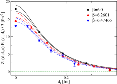
Figure 5: Same data as in Fig. 4, together with $1\sigma$ bands obtained from the combined fit described in the text.

In this approach the following parametrization of the longitudinal component of chromoelectric field inside the flux tube is used:

$$E_{L}^{(R)}(d_{t})=\frac{\phi}{2\pi}\frac{\mu^{2}}{\alpha}\frac{K_{0}\big{(}\sqrt{\mu^{2}d_{t}^{2}+\alpha^{2}}~{}\big{)}}{K_{1}(\alpha)}\ ,$$ (24)

where $K_{0}$, $K_{1}$ are modified Bessel functions of the second kind, and $\phi,\alpha$ and $\mu$ are fit parameters. This is the “dual” version of the parametrization introduced in Clem for the longitudinal magnetic field inside a vortex line in type II superconductors. The parameter $\mu$ is just the inverse of the penetration length, $\mu=1/\lambda$, while the relation between the fit parameters in Eq. (24) and the coherence length is less direct: it can be shown (see Clem ) that the Ginzburg-Landau parameter $\kappa=\lambda/\xi$ is related to $\alpha$ by the relation

$$\kappa=\frac{\sqrt{2}}{\alpha}\sqrt{1-\frac{K_{0}^{2}(\alpha)}{K_{1}^{2}(\alpha)}}\ .$$ (25)

Values of $\kappa$ smaller than $1/\sqrt{2}$ correspond to superconductors of type I, while $\kappa>1/\sqrt{2}$ for type II superconductors (see e.g. Tinkham ).

If we try to fit each of the fixed $\beta$ data sets shown in Fig. 4 by using the parametrization in Eq. (24), we immediately realize that the quality of the fits degrades as the coupling is increased. This is a consequence of the previously noted fact that data points at $d_{t}=0$ and at $d_{t}>0$ scale to the continuum in different ways, due to the different logarithmic divergences in the two cases. If on the other hand we simply discard the point at $d_{t}=0$ from each of our data sets, the precision of our data is not enough for the fit to provide significant information on $\alpha$, and consequently on the Ginzburg-Landau parameter $\kappa$.

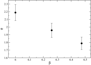
Figure 6: Continuum scaling of the parameters $\phi$ obtained by using the combined fit described in the text.

We thus decided to perform a combined fit of all our data at $d_{t}>0$ keeping three different $\phi$ parameters, corresponding to the three lattice spacings used, since $\phi$ is sensitive to the multiplicative renormalization $Z_{1}(a,d)$. Using $c_{a}=-0.45$ we obtain the best fit shown in Fig. 5 and the final results for the superconductivity parameters are

$$\frac{1}{\lambda}=\mu=7.4(6)\mathrm{fm}^{-1},\quad\alpha=0.7(2),\quad\kappa=1.8(6)\ ,$$ (26)

while the values obtained for the $\phi$s parameters shown in Fig. 6. The $\chi^{2}$ test for this fit gives $\chi^{2}/\mathrm{dof}=16/10$ that is somehow large but still acceptable, and the final results are almost unchanged also for $c_{a}=-0.47$ and $c_{a}=-0.43$, which means that the uncertainty in $c_{a}$ is not the main source of error in our final results.

IV Conclusions

In this paper we presented the results of our study of the longitudinal chromoelectric component of the color flux tube, performed by using the connected correlator. Measures were carried out by means of stochastically exact techniques, without any smoothing, in order to investigate the possibility of using the connected correlator $\rho_{conn}$ in a coherent field-theoretical setup.

We first investigated the renormalization properties of $\rho_{conn}$, showing that it is multiplicatively renormalizable, and reducing the problem of its renormalization to the determination of three renormalization constants. One of these constants (denoted by $c_{a}$) is related to linear divergences, while the other two take care of the logarithmic divergences in the cases $d_{t}=0$ and $d_{t}\neq 0$ respectively.

We then fixed the value of $c_{a}$, by studying the $\beta$ dependence (at fixed temperature) of the Polyakov loop in the adjoint representation. Using the value of $c_{a}$ obtained in this way ($c_{a}=-0.45(2)$), we removed linear divergences from $\rho_{conn}$, obtaining the results shown in Fig. 4. While it is important to stress that these data are still not renormalized (since logarithmic divergences have not been removed), it is possible to extract from them quantities of direct physical interest.

In particular, starting from the functional form of the longitudinal chromoelectric field, we evaluated the coherence length $\xi$ and the penetration length $\lambda$ of the dual superconductor model. The numerical values of these quantities, extracted using a flux tube of length $d\simeq 0.37\,\mathrm{fm}$, are reported in Eq. (26). The values of $\xi$, $\lambda$ and $\kappa$ reported in the literature have been obtained using quite larger $d$ values, so that a direct comparison can not be performed. It is nevertheless interesting to note that our estimate of the penetration length $\lambda$ is in good agreement with previous determinations. Our Ginzburg-Landau parameter (and consequently our coherence length) is instead quite different from the one obtained in similar studies carried out by using smoothing Cea:2012qw ; Cea:2014uja (where $\kappa\approx 0.2$ was found), being closer to older results suggesting the $SU(2)$ vacuum to be at the boundary between type I and type II superconductivity Bali:1997cp ; Gubarev:1999yp ; Koma:2003hv ; Haymaker:2005py ; Chernodub:2005gz ; DAlessandro:2006hfn .

This result suggests that smoothing could introduce some systematics in the determination of the flux tube profile, and we get the following intuitive picture: $\xi$ is the typical scale of the bulk of the flux tube, which broadens under smoothing, while $\lambda$ is related to the large distance behaviour of the tails, which is almost unaffected by smoothing. As a consequence we expect smoothing to leave almost unaltered $\lambda$ and to decrease $\kappa=\lambda/\xi$.

While this picture seems appealing we also have to keep in mind the limitations of our computation: first of all our determination of $\kappa$ has a $30\%$ relative error, so this effect could just be a statistical fluctuation. Moreover the distance between the Polyakov loops used to extract $\xi$ and $\lambda$ was only about $0.37\,\mathrm{fm}$, which is surely not asymptotically large; as a consequence a contamination from the Coulomb component of the flux tube is possible (see Baker:2018mhw for a discussion on this point).

As noted before, most of the results reported in the literature adopt quite larger values of $d$ to extract $\lambda$ and $\xi$, so that a fair comparison with our results Eq. (26) is not possible. However a direct comparison can be made between Fig. 6 above and Fig. 2 of Cea:2014uja , where the flux tube profile is reported for the case $\beta=6.0$ and $d=4a$ (computed by using a $20^{4}$ lattice): the half-width at half-maximum of the flux tube in Fig. 6 (for $\beta=6.0$) is about $0.12\,\mathrm{fm}$, while the corresponding value extracted from Fig. 2 of Cea:2014uja is about $0.23\,\mathrm{fm}$. This is consistent with the possibility that smoothing increases the thickness of the flux tube.

A more complete investigation of the long distance structure of the flux tube, performed by using higher statistics and larger values of the distance between the Polyakov loops, is surely matter for further studies, just as the determination of the renormalization constants associated to the logarithmic diverges of $\rho_{conn}$.

- (1) M. Fukugita and T. Niuya, Phys. Lett. 132B, 374 (1983).
- (2) J. W. Flower and S. W. Otto, Phys. Lett. 160B, 128 (1985).
- (3) J. Wosiek and R. W. Haymaker, Phys. Rev. D 36, 3297 (1987).
- (4) R. Sommer, Nucl. Phys. B 291, 673 (1987).
- (5) A. Di Giacomo, M. Maggiore and S. Olejnik, Phys. Lett. B 236, 199 (1990).
- (6) A. Di Giacomo, M. Maggiore and S. Olejnik, Nucl. Phys. B 347, 441 (1990).
- (7) G. S. Bali, K. Schilling and C. Schlichter, Phys. Rev. D 51, 5165 (1995) [hep-lat/9409005].
- (8) R. W. Haymaker, V. Singh, Y. C. Peng and J. Wosiek, Phys. Rev. D 53, 389 (1996) [hep-lat/9406021].
- (9) P. Cea and L. Cosmai, Phys. Rev. D 52, 5152 (1995) [hep-lat/9504008].
- (10) F. Okiharu and R. M. Woloshyn, Nucl. Phys. Proc. Suppl. 129, 745 (2004) [hep-lat/0310007].
- (11) F. Bissey, F. G. Cao, A. R. Kitson, A. I. Signal, D. B. Leinweber, B. G. Lasscock and A. G. Williams, Phys. Rev. D 76, 114512 (2007) [hep-lat/0606016].
- (12) P. Bicudo, N. Cardoso and M. Cardoso, Prog. Part. Nucl. Phys. 67, 440 (2012) [arXiv:1111.0334 [hep-lat]].
- (13) A. S. Bakry, X. Chen and P. M. Zhang, Phys. Rev. D 91, 114506 (2015) [arXiv:1412.3568 [hep-lat]].
- (14) J. B. Kogut and L. Susskind, Phys. Rev. D 11, 395 (1975).
- (15) K. Osterwalder and E. Seiler, Annals Phys. 110, 440 (1978).
- (16) M. Luscher, G. Munster and P. Weisz, Nucl. Phys. B 180, 1 (1981).
- (17) A. Allais and M. Caselle, JHEP 0901, 073 (2009) [arXiv:0812.0284 [hep-lat]].
- (18) F. Gliozzi, M. Pepe and U.-J. Wiese, Phys. Rev. Lett. 104, 232001 (2010) [arXiv:1002.4888 [hep-lat]].
- (19) F. Gliozzi, M. Pepe and U.-J. Wiese, JHEP 1101, 057 (2011) [arXiv:1010.1373 [hep-lat]].
- (20) N. Cardoso, M. Cardoso and P. Bicudo, Phys. Rev. D 88, 054504 (2013) [arXiv:1302.3633 [hep-lat]].
- (21) A. Amado, N. Cardoso and P. Bicudo, arXiv:1309.3859 [hep-lat].
- (22) M. Caselle, M. Panero and D. Vadacchino, JHEP 1602, 180 (2016) [arXiv:1601.07455 [hep-lat]].
- (23) M. S. Cardaci, P. Cea, L. Cosmai, R. Falcone and A. Papa, Phys. Rev. D 83, 014502 (2011) [arXiv:1011.5803 [hep-lat]].
- (24) P. Cea, L. Cosmai and A. Papa, Phys. Rev. D 86, 054501 (2012) [arXiv:1208.1362 [hep-lat]].
- (25) P. Cea, L. Cosmai, F. Cuteri and A. Papa, Phys. Rev. D 89, 094505 (2014) [arXiv:1404.1172 [hep-lat]].
- (26) P. Cea, L. Cosmai, F. Cuteri and A. Papa, JHEP 1606, 033 (2016) [arXiv:1511.01783 [hep-lat]].
- (27) M. Baker, P. Cea, V. Chelnokov, L. Cosmai, F. Cuteri and A. Papa, arXiv:1810.07133 [hep-lat].
- (28) P. Cea, L. Cosmai, F. Cuteri and A. Papa, Phys. Rev. D 95, 114511 (2017) [arXiv:1702.06437 [hep-lat]].
- (29) C. Bonati, S. Calì, M. D’Elia, M. Mesiti, F. Negro, A. Rucci and F. Sanfilippo, Phys. Rev. D 98, 054501 (2018) [arXiv:1807.01673 [hep-lat]].
- (30) M. Cè, L. Giusti and S. Schaefer, Phys. Rev. D 95, 034503 (2017) [arXiv:1609.02419 [hep-lat]].
- (31) G. Parisi, R. Petronzio and F. Rapuano, Phys. Lett. 128B, 418 (1983).
- (32) M. Luscher and P. Weisz, JHEP 0109, 010 (2001) [hep-lat/0108014].
- (33) M. Berwein, N. Brambilla, J. Ghiglieri and A. Vairo, JHEP 1303, 069 (2013) [arXiv:1212.4413 [hep-th]].
- (34) M. Berwein, N. Brambilla and A. Vairo, Phys. Part. Nucl. 45, 656 (2014) [arXiv:1312.6651 [hep-th]].
- (35) A. M. Polyakov, Nucl. Phys. B 164, 171 (1980).
- (36) V. S. Dotsenko and S. N. Vergeles, Nucl. Phys. B 169, 527 (1980).
- (37) R. A. Brandt, F. Neri and M. a. Sato, Phys. Rev. D 24, 879 (1981).
- (38) E. Gardi, E. Laenen, G. Stavenga and C. D. White, JHEP 1011, 155 (2010) [arXiv:1008.0098 [hep-ph]].
- (39) E. Gardi, J. M. Smillie and C. D. White, JHEP 1306, 088 (2013) [arXiv:1304.7040 [hep-ph]].
- (40) K. G. Wilson, Phys. Rev. D 10, 2445 (1974).
- (41) S. Necco and R. Sommer, Nucl. Phys. B 622, 328 (2002) [hep-lat/0108008].
- (42) R. Sommer, Nucl. Phys. B 411, 839 (1994) [hep-lat/9310022].
- (43) J. Fingberg, U. M. Heller and F. Karsch, Nucl. Phys. B 392, 493 (1993) [hep-lat/9208012].
- (44) S. Mandelstam, Phys. Rept. 23, 245 (1976).
- (45) G. Parisi, Phys. Rev. D 11, 970 (1975).
- (46) G. ’t Hooft “Gauge Theory for Strong Interactions”, in A. Zichichi (Ed.) “New Phenomena in Subnuclear Physics” Subnucl. Ser. 13 (1977).
- (47) J. R. Clem, J. Low Temp. Phys. 18, 427 (1975).
- (48) M. Tinkham “Introduction to superconductivity”, McGraw-Hill (1996).
- (49) G. S. Bali, C. Schlichter and K. Schilling, Prog. Theor. Phys. Suppl. 131, 645 (1998) [hep-lat/9802005].
- (50) F. V. Gubarev, E. M. Ilgenfritz, M. I. Polikarpov and T. Suzuki, Phys. Lett. B 468, 134 (1999) [hep-lat/9909099].
- (51) Y. Koma, M. Koma, E. M. Ilgenfritz and T. Suzuki, Phys. Rev. D 68, 114504 (2003) [hep-lat/0308008].
- (52) R. W. Haymaker and T. Matsuki, Phys. Rev. D 75, 014501 (2007) [hep-lat/0505019].
- (53) M. N. Chernodub, K. Ishiguro, Y. Mori, Y. Nakamura, M. I. Polikarpov, T. Sekido, T. Suzuki and V. I. Zakharov, Phys. Rev. D 72, 074505 (2005) [hep-lat/0508004].
- (54) A. D’Alessandro, M. D’Elia and L. Tagliacozzo, Nucl. Phys. B 774, 168 (2007) [hep-lat/0607014].