Temporal changes in stimulus perception improve bio-inspired source seeking

Abstract

Braitenberg vehicles are well known qualitative models of sensor driven animal source seeking (biological taxes) that locally navigate a stimulus function. These models ultimately depend on the perceived stimulus values, while there is biological evidence that animals also use the temporal changes in the stimulus as information source for taxis behaviour. The time evolution of the stimulus values depends on the agent’s (animal or robot) velocity, while simultaneously the velocity is typically the variable to control. This circular dependency appears, for instance, when using optical flow to control the motion of a robot, and it is solved by fixing the forward speed while controlling only the steering rate. This paper presents a new mathematical model of a bio-inspired source seeking controller that includes the rate of change of the stimulus in the velocity control mechanism. The above mentioned circular dependency results in a closed-loop model represented by a set of differential-algebraic equations (DAEs), which can be converted to non-linear ordinary differential equations (ODEs) under some assumptions. Theoretical results of the model analysis show that including a term dependent on the temporal evolution of the stimulus improves the behaviour of the closed-loop system compared to simply using the stimulus values. We illustrate the theoretical results through a set of simulations.

I Introduction

Braitenberg vehicles [1] are a well known model of animal navigation in robotics. They constitute a set of bio-inspired navigation primitives [2] to move towards or away from stimulus, known in biology as taxes [3]. Whilst in the seminal work of Braitenberg these models defined steering control principles based on direct perception of the stimulus, there is evidence in the literature showing that animals also use the temporal change of the perceived stimulus to drive their movement [4]. However, the dynamics of the stimulus depends on the movement of the animal, as for the same static stimulus faster speed implies faster perceived temporal changes. In this paper we develop a new mathematical model of Braitenberg vehicle 3a, that achieves target seeking, and includes steering control based on the temporal evolution of the perceived stimulus. Because these wheeled vehicles rely on the unicycle motion model, the resulting closed-loop equations are a set of non-linear differential-algebraic equations, which can be converted (under some conditions) to standard non-linear differential equations. The formal analysis of the model allows to identify the equilibrium points and some stability properties of this special controller, and shows that it generates better trajectories compared to the original Braitenberg 3a vehicle. To the best of our knowledge this work presents the first attempt to analyse theoretically a velocity-based sensor driven navigation mechanism that depends on the velocity of the robot itself. This work has implications for navigation mechanism based on information dependent on the temporal changes like the optical flow or event cameras, where the perception depends on the movement of the robot.

Braitenberg vehicles are typically used in the literature with unconventional sensors (i.e. sensors other than range or positioning sensors) to implement local navigation using, among others; sound (phonotaxis), light (phototaxis) or chemical (chemotaxis) stimuli, but there are also use cases for local navigation using range sensors. The work in [5] presents a model of the rat’s peripheral and central auditory system that enables the authors to implement phonotaxis through a Braitenberg vehicle 3a to control the motion of a mobile robot. A model of the auditory system of lizards was presented in [6] [7] to control a mobile robot performing phonotaxis using Braitenberg vehicle 2b. The phonotaxis behaviour of female crickets towards male crickets is mimicked in a series of papers [8] [9] [10] that use the principles of Braitenberg vehicles 2a and 3b to design spiking neural networks. Their experimental results show that their robot achieves excellent performance even in outdoor scenarios with the use of whegs (wheeled legs). One of the earlier works in robotic chemotaxis (localisation of an odour source) analysed experimentally the behaviour of vehicles 3a and 3b [11]. While the connection between the sensors and the wheels was linearly proportional, the chemical concentration readings were continuously normalised due to the saturation and dynamic effects of the chemical sensing technology.

The recent development and use of other unconventional sensing modalities has also lead to the use of Braitenberg vehicles and their principles on non-wheeled robots. A fish robot endowed with pressure sensors imitating the fish lateral line used Braitenberg vehicle 2b to implement rheotaxis [12], the alignment of the fish body with a current or flow. Compared to other control mechanisms, the deviation of the robot using this bio-inspired mechanism with respect to the flow direction was significantly lower. Moreover, because the movement of the fish-robot affected the measurements of the lateral line, this work constitutes an experimental example of the control mechanism staying stable under movement induced sensing dynamics. Another application of the principles of Braitenberg vehicles to fish robotics is the work presented in [13]. In this work, the motion of an electric fish-robot is controlled by the differences between the currents sensed by electrodes located on the sides of the robot. The robot moves towards conductive objects in a pond, avoiding isolating obstacles. Similarly to the previous fish robot, the movement occurs in two dimensions, yet in the case of the electric fish the robot is rigid and controlled through a rod. Another example where Braitenberg vehicles are applied to non-wheeled robots is the work presented in [14], where a simulated snake robot is controlled to approach a light source by generating modulated undulatory signals in its joints. One type of unconventional sensor that has recently gained traction is the event cameras, which are used in [15] in combination with a Braitenberg vehicle 2b to implement visual obstacle avoidance in a wheeled robot using neuromorphic hardware.

As we mentioned, Braitenberg vehicles are often used with unconventional sensors, although some instances can be found that use range sensors instead. In [16] a Braitenberg vehicles were used for target acquisition of a light source – phototaxis through vehicle 3a –, and infrared sensor based obstacle avoidance – through vehicle 2b. This work shows that proximity sensors can be also used in conjunction with this bio-inspired local navigation technique. Furthermore, this work inspired an implementation of a Braitenberg vehicle based on the readings of a laser scanner to estimate the free area around a robot [17]. This paper also proves that the motion of vehicle 2b can lead to chaotic trajectories, a feature exploited in [18] to implement area coverage in a simulated environment with a stimulus similar to the free area around a robot. The chaotic coverage strategy outperforms random walks and Levy walks.

As we saw, Braitenberg vehicles have been used with multiple sensor and different robot types (mainly wheeled robots) but always using the originally proposed instantaneous sensor readings or low pass filtered signals. The main contribution of this paper is to extend this successful control mechanism with a controller dependent on the dynamic changes of the stimulus perceived by the vehicle. Furthermore, we analyse the stability of the resulting controller and show that it is stable and outperforms the original model. This work is inspired by the biological findings supporting the use of rates of change of perception for control and the successful experimental results obtained in simulations motivated by these biological findings [19]. The rest of the paper is organised as follows. Section II reviews the definitions and standard assumptions of Braitenberg vehicle 3a and presents the new control mechanism that includes the temporal change of the stimulus. This section also analyses the stability of the model under some assumptions. Section III presents a series of simulations that illustrate the main theoretical results obtained. Finally, section IV presents some conclusions and future work.

II Dynamic model of Braitenberg vehicle 3a

Let’s assume a Braitenberg vehicle 3a with two sensors and a direct connection between the sensors and the motors as shown in figure 1. The state of the vehicle in the 2D plane can be represented by the vector $\mathbf{X}=[x,y,\theta]$, and we will denote just the Cartesian coordinates by $\mathbf{x}=[x,y]$. The selected $x$ and $y$ coordinates correspond to the middle point between the sensors, and we define the orthogonal reference system linked to the front of the vehicle as $\hat{e}=[\cos\theta,\sin\theta]$ and $\hat{e}_{p}=[-\sin\theta,\cos\theta]$.

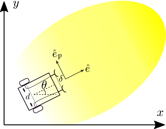
Figure 1: Representation of the qualitative model of Braitenberg vehicle 3a

We assume a smooth positive stimulus $S(\mathbf{x})$ exists in the plane, i.e. $S(\mathbf{x})>0$ for all $\mathbf{x}\in\Re^{2}$ and $S(\mathbf{x})$ is of class $C^{\infty}$. Without loss of generality we can assume that the maximum of the stimulus occurs at $\mathbf{x}=\mathbf{0}$, i.e. $S(\mathbf{0})>S(\mathbf{x})$ for all $\mathbf{x}\in\Re^{2}$. Defining the distance between the sensors is $\delta$, we can express the positions of the right and left sensors as $\mathbf{x}_{r}=\mathbf{x}-\frac{\delta}{2}\hat{e}_{p}$ $\mathbf{x}_{l}=\mathbf{x}+\frac{\delta}{2}\hat{e}_{p}$ respectively. Therefore, the value of $S(\mathbf{x})$ measured by these sensors will be $S(\mathbf{x}_{r})$ and $S(\mathbf{x}_{l}$. According to the standard model of vehicle 3a [20] the velocity of each wheel is a decreasing function $F(s)$ of the stimulus perceived by the sensor located on the same side of the vehicle. We will assume the vehicle only moves forward $F(s)>0$, while $F(s)$ being decreasing implies $F^{\prime}(s)<0$. Therefore, the velocity of each wheel is in general a non-linear function of the stimulus $v=F(S(\mathbf{x}))$ (or $v=F(\mathbf{x})$ for short). Because we want the vehicle to reach the maximum and stop there, $F(s)$ has to be chosen such that $F(S(\mathbf{0}))=0$. However, in this paper we will consider the case in which the velocity also depends on the temporal rate of change of the stimulus, i.e. $v=F(s,\dot{s})$, and as a first step we will assume that the contribution of the stimulus derivative is additive, which allows is to state the velocities of each wheel as:

$$v_{r} = F(S(\mathbf{x}_{r}))+G(\dot{S}(\mathbf{x}_{l}))$$

$$v_{l} = F(S(\mathbf{x}_{l}))+G(\dot{S}(\mathbf{x}_{r}))$$ (1)

where $G(\dot{s})$ can be a non-linear function with the constraint $G(0)=0$ for the vehicle to stop at the maximum. It is worth noting that the effects on the speed of the temporal derivative of the stimulus is contralateral, i.e. derivative of $S(\mathbf{x})$ on the right sensor effects the velocity of the left wheel, and vice-versa.

Substituting the expressions for $\mathbf{x}_{r}$ and $\mathbf{x}_{l}$ in equations (1), we can state the speeds of the right and left wheels ($v_{r}$ and $v_{l}$) as a function of the state of the vehicle (the Cartesian coordinates $\mathbf{x}$ and its orientation $\theta$) and the distance between the sensors $\delta$. Furthermore, we can approximate the compound functions $F(S(\cdot))$ and $G(S(\cdot))$ as first order Taylor series around $\mathbf{x}$ assuming $\delta$ is small relative to changes in $S(\mathbf{x})$, and then compute the forward speed of the vehicle, $v=\frac{v_{r}+v_{l}}{2}$, and its turning rate $\omega=\frac{v_{r}-v_{l}}{d}$, where $d$ is the wheelbase. This leads to the following speeds:

$$v = F(S(\mathbf{x}))+G(\nabla S^{T}\dot{\mathbf{x}})$$

$$\omega = -\frac{\delta}{d}\nabla F(S(\mathbf{x}))^{T}\hat{e}_{p}$$ (2)

$$\quad-\frac{\delta}{d}G^{\prime}(\nabla S^{T}\dot{\mathbf{x}})\left[\dot{\theta}\nabla S^{T}\hat{e}-\hat{e}_{p}^{T}HS\dot{\mathbf{x}}\right]$$

where $\nabla F(S(\mathbf{x}))$ is the gradient of the compound function $F(S(\mathbf{x}))$, $\nabla S$ and $HS$ denote the gradient and Hessian matrix of the stimulus respectively, and we used the fact that $\dot{S}(\mathbf{x})=\nabla S^{T}\dot{\mathbf{x}}$.

Introducing equations (2) in the unicycle model we obtain the closed-loop equations of motion of the dynamic Braitenberg vehicle 3a:

$$\dot{x} = F(S(\mathbf{x}))\cos\theta+G(\nabla S^{T}\dot{\mathbf{x}})\cos\theta$$

$$\dot{y} = F(S(\mathbf{x}))\sin\theta+G(\nabla S^{T}\dot{\mathbf{x}})\sin\theta$$

$$\dot{\theta} = -\frac{\delta}{d}\nabla F(S(\mathbf{x}))\hat{e}_{p}$$ (3)

$$-\frac{\delta}{d}G^{\prime}(\nabla S^{T}\dot{\mathbf{x}})\left[\dot{\theta}\nabla S^{T}\hat{e}-\hat{e}_{p}HS\dot{\mathbf{x}}\right]$$

It is worth noting that while the model of Braitenberg vehicle 3a is stated as a system of non-linear ordinary differential equations, equations (3) correspond to a differential-algebraic system of equations (DAE) as the time derivative of the state $\dot{\mathbf{X}}=[\dot{\mathbf{x}},\dot{\theta}]$ ($\dot{\mathbf{x}}=[\dot{x},\dot{y}]$) is on the r.h.s of the equations. DAEs are much more complex to solve than ODEs, as, for instance, the set of meaningful initial conditions could be restricted. Therefore, we will make some assumptions that will allow us to analyse the closed-loop behaviour analytically.

II-A From Differential Algebraic to Ordinary Differential Equations

Deriving analytic results from equations (3) can be challenging, however, the DAEs can be converted into a system of ordinary differential equations if we assume that the function $G(\dot{S})$ is linear, i.e $G(\dot{S})=\alpha\dot{S}$, which is the simplest function fulfilling the condition $G(0)=0$. It can be seen that the closed-loop equations can be stated as $\dot{\mathbf{X}}=\mathcal{F}(\mathbf{X})+\alpha A(\mathbf{X})\dot{\mathbf{X}}$, where the derivative of the state on the r.h.s is multiplied by the matrix:

$$A = \left[\begin{array}[]{ccc}S_{x}\cos\theta&S_{y}\cos\theta&0\\ S_{x}\sin\theta&S_{y}\sin\theta&0\\ \frac{\delta}{d}\hat{e}_{p}^{T}HS|_{x}&\frac{\delta}{d}\hat{e}_{p}^{T}HS|_{y}&-\frac{\delta}{d}\nabla S^{T}\hat{e}\end{array}\right]$$ (7)

where $S_{x}=\frac{\partial S}{\partial x}$, $S_{y}=\frac{\partial S}{\partial y}$, and $\hat{e}_{p}^{T}HS|_{x}$ $\hat{e}_{p}^{T}HS|_{y}$ represent the $x$ and $y$ components of the row vector $\hat{e}_{p}^{T}HS$, the result of multiplying $\hat{e}_{p}^{T}$ by the Hessian matrix of $S(\mathbf{x})$. The vector flow $\mathcal{F}(\mathbf{X})$ is formed from the terms on the r.h.s. of the equation not involving the time derivatives of the state $\mathbf{X}$.

The motion equations of the vehicle (3) can be stated as $\dot{\mathbf{X}}=[I-\alpha A(\mathbf{X})]^{-1}\mathcal{F}(\mathbf{X})$, which is an ordinary differential equation, assuming the matrix $I-\alpha A$ is not singular. Therefore, the determinant of $I-\alpha A$:

$$|I-\alpha A| = -\frac{1}{d}\left[\alpha\nabla S^{T}\hat{e}-1\right]\left[\alpha\delta\nabla S^{T}\hat{e}+d\right]$$ (8)

should be different than zero, which provides us with the conditions under which the DAE (3) can be turned into the ODE $\dot{\mathbf{X}}=[I-\alpha A(\mathbf{X})]^{-1}\mathcal{F}(\mathbf{X})$. Specifically, the determinant vanishes when $\nabla S^{T}\hat{e}=\frac{1}{\alpha}$ or when $\nabla S^{T}\hat{e}=-\frac{d}{\delta\alpha}$. Interestingly, if $\delta=d$ both conditions can be stated as $|\nabla S^{T}\hat{e}|=\frac{1}{\alpha}$ (assuming $\alpha>0$, which will be justified below), i.e. the inverse of $\alpha$ should be different from the directional gradient in the direction of motion along the trajectory of the vehicle. This leads to a constrain for the possible values of $\alpha$, namely $\alpha\neq\frac{1}{\nabla S^{T}\hat{e}}$. If this condition is fulfilled, the closed-loop motion equations corresponding to the dynamic Braitenberg vehicle 3a are:

$$\dot{x} = \frac{F(S(\mathbf{x}))\cos\theta}{1-\alpha\nabla S^{T}\hat{e}}$$

$$\dot{y} = \frac{F(S(\mathbf{x}))\sin\theta}{1-\alpha\nabla S^{T}\hat{e}}$$

$$\dot{\theta} = -\frac{\delta\nabla F^{T}\hat{e}_{p}}{(d+\alpha\delta\nabla S^{T}\hat{e})}$$ (9)

$$-\frac{\alpha\delta F(S(\mathbf{x}))\hat{e}_{p}^{T}HS\hat{e}}{(\alpha\nabla S^{T}\hat{e}-1)(d+\alpha\delta\nabla S^{T}\hat{e})}$$

These equations are similar to the closed-loop model of Braitenberg vehicle 3a [20], in fact the original model can be obtained by simply setting $\alpha=0$. Moreover, it can be shown that they have an equilibrium point at the origin – the maximum of $S(\mathbf{x})$ – since $\nabla S(\mathbf{0})=\mathbf{0}$ and $F(S(\mathbf{0}))=0$, which implies $\dot{x}=0$, $\dot{y}=0$ and $\dot{\theta}=0$. The analysis of the stability of the equilibrium point in the case of Braitenberg vehicle 3a is presented elsewhere, but for the case at hand the stability properties could change due to the additional term in the equation for $\dot{\theta}$.

The condition on the determinant of $I-\alpha A(\mathbf{X})$ for the inverse matrix to exist is also reflected in the equations, as when $|\nabla S|=-\frac{1}{\alpha}$ or $|\nabla S|=-\frac{d}{\alpha\delta}$ the denominators of the three dynamic equations would go to zero generating possibly unbounded speeds. So the parameter $\alpha$ has to be chosen carefully considering the possible values of the norm of the stimulus gradient. While the equation for the angular variable $\dot{\theta}$ is hard to analyse at first sight, the equations for $\dot{x}$ and $\dot{y}$ provide a new insight on the effect of the dynamic controller over the closed-loop behaviour. First it is worth noting that the forward speed of the vehicle is $v=\frac{F(S(\mathbf{x}))}{1-\alpha\nabla S^{T}\hat{e}}$, where $\hat{e}$ is the vector pointing in the direction of the vehicle and $\nabla S$ points in the direction of increasing stimulus. If the vehicle points exactly in the direction of $\nabla S$, the dot product of the two vectors corresponds to the norm of the gradient, i.e. $\nabla S\hat{e}=|\nabla S|$, and if it points in the direction opposite to the stimulus gradient it will be $\nabla S\hat{e}=-|\nabla S|$. Now let’s assume $\alpha>0$ and define $\nabla S^{*}$ as the gradient with the largest norm in the environment or the domain where $S(\mathbf{x})$ is defined. If we impose the additional condition on $\alpha$ $0<\alpha<\frac{1}{|\nabla S^{*}|}$ the term $\alpha\nabla S^{T}\hat{e}$ will be positive and smaller than one when the vehicle points in the direction of increasing $S(\mathbf{x})$. The overall effect compared to the Braitenberg vehicle 3a is to increase the forward speed since the denominator of $v$ becomes smaller than one. On the other hand, if the vehicle points in the direction opposite to the gradient, the dot product $\nabla S^{T}\hat{e}$ will be negative, making the denominator of the forward speed larger than one, which effectively reduces the forward speed. This is a highly interesting effect of introducing the temporal rate of change of the stimulus in the velocity control of the vehicle, as it makes the vehicle to move faster when it faces the source, while reduces its speed when the source is on its back. Analysing the behaviour of the the equation for $\dot{\theta}$ is not trivial since in the dynamic case there is a new term which could change the sign of the original rotation speed (for which stability conditions can be derived [21]). In the next section we will take a closer look at the stability of the system under the additional assumption of parabolically symmetric stimulus.

II-B Motion under parabolic stimulus

In this section we will assume the stimulus has parabolic symmetry of the form $S(\mathbf{x})=S(\mathbf{x}^{T}D\mathbf{x})$ where $D=diag(\sigma_{x},\sigma_{y})$ is a positive definite diagonal matrix. This will allows us to analyse the stability and derive more results on the trajectories of the closed-loop controller. The assumption holds for any smooth stimulus close enough to the source. Moreover, since the reference system can be defined arbitrarily we can rotate the $x$ and $y$ axis to be aligned with the principal axis of the stimulus. Under these assumptions the gradient of the stimulus can be written as $\nabla S=2S^{\prime}(\mathbf{x}^{T}D\mathbf{x})D\mathbf{x}$, where $S^{\prime}(\cdot)$ is the derivative of $S(\cdot)$ w.r.t its argument, with $S^{\prime}(\cdot)<0$ because the stimulus to grows towards the source (located at $\mathbf{x}=\mathbf{0}$). The Hessian matrix of this stimulus is $HS(\mathbf{x})=4S^{\prime\prime}(\mathbf{x}^{T}D\mathbf{x})D\mathbf{x}\mathbf{x}^{T}D+2S^{\prime}(\mathbf{x}^{T}D\mathbf{x})D$ which is negative definite at the origin, as the origin is a maximum. Using the additional condition on the control function $F(S(\mathbf{0}))=0$ and evaluating $\dot{x}$, $\dot{y}$ and $\dot{\theta}$, eq. (9) at the stimulus maximum we obtain the following condition for an equilibrium point to appear $\hat{e}_{p}^{T}D\hat{e}=0$, which is satisfied for all $\theta$ if $\sigma_{x}=\sigma_{y}$, or for $\theta=0$, $\theta=\pi$ and $\theta=\pm\pi/2$ if $\sigma_{x}\neq\sigma_{y}$. So the closed-loop system has infinite equilibrium points for circularly symmetric stimuli ($\sigma_{x}=\sigma_{y}$), or four equilibrium points for parabolically symmetric stimuli $\sigma_{x}\neq\sigma_{y}$.

From the ODE form of the closed-loop equations we can also find an analytic solution to the equations. Just like the standard Braitenberg vehicle, when the initial pose of the vehicle falls on, and is aligned with, the main axis of the stimulus (lines $x=0$ and $y=0$ with heading $\theta=0$ or $\theta=\pi$ and $\theta=\pm\frac{\pi}{2}$ respectively) the vehicle follows a straight line trajectory towards (or away from) the maximum of the stimulus. Taking, for instance $x(0)=-x_{0}$, $y(0)=0$ and $\theta(0)=0$ as a starting pose we get for the $y$ coordinate that $\dot{y}=0$ and for the $x$ coordinate:

$$\dot{x} = \frac{F(S(\sigma_{x}x^{2}))}{1-2\alpha S^{\prime}(\sigma_{x}x^{2})\sigma_{x}x}$$ (10)

while the equation of $\theta$ becomes $\dot{\theta}=0$ since $\nabla F$ is perpendicular to $\hat{e}_{p}$ and $\hat{e}_{p}HS\hat{e}=0$ (for $\theta=0$ $\hat{e}=[1,0]$ and $\hat{e}_{p}=[0,1]$). Therefore, the trajectory is indeed a straight line with the evolution of $x$ given by equation (10).

Having this particular solution to the system of non-linear equations (9) allows us to linerarise the system around that trajectory and to check the evolution of the nearby trajectories with increments $\Delta\mathbf{X}$ following $\Delta\mathbf{\dot{X}}=M(t)\Delta\mathbf{X}$. The linearised system is a time varying linear system, and the eigenvalues of the matrix $M(t)$ – which depend on the solution of equation (10) – provide information on the stability of the non-linear system, i.e. first Lyapunov criterion applied to a non-constant trajectory. Because the linearised system is three dimensional, at least one eigenvalue will be real, while the other two could be complex conjugates, which is the case when $\alpha=0$, i.e. the standard Braitenberg vehicle under parabolically symmetric stimuli [21]. If we denote $F=F(S(\sigma_{x}x^{2}))$, $F^{\prime}=F^{\prime}(S(\sigma_{x}x^{2}))$, $S^{\prime}=S^{\prime}(\sigma_{x}x^{2})$, $S^{\prime\prime}=S^{\prime\prime}(\sigma_{x}x^{2})$, $\Delta_{1}=1-2\alpha\sigma_{x}xS^{\prime}$ and $\Delta_{2}=d-2\alpha\delta\sigma_{x}xS^{\prime}$ the real eigenvalue of the matrix $M(t)$ can be written as:

$$\lambda_{1} = \frac{2\sigma_{x}xF^{\prime}S^{\prime}}{\Delta_{1}}+\frac{2\alpha\sigma_{x}F[S^{\prime}+2\sigma_{x}x^{2}S^{\prime\prime}]}{\Delta_{1}^{2}}$$

while the real part of the complex conjugate eigenvalues is:

$$Re[\lambda_{2,3}] = \frac{\delta\sigma_{x}xF^{\prime}S^{\prime}}{\Delta_{2}}+\frac{\alpha\delta F[S^{\prime}[\sigma_{x}-\sigma_{y}]+2S^{\prime\prime}\sigma_{x}^{2}x^{2}]}{\Delta_{1}\Delta_{2}}$$

where $\sigma_{x}>0$, $x<0$, $F>0$, $F^{\prime}<0$ and $S^{\prime}<0$. It can be seen that a sufficient condition for the real the eigenvalue to be negative is $S^{\prime}+2\sigma_{x}x^{2}S^{\prime\prime}<0$, but $\lambda_{1}$ could be negative even if this condition is not met. Moreover, because $0<\Delta_{1}<1$ from the condition imposed on $\alpha$, $\lambda_{1}$ will be more negative than the corresponding eigenvalue for the standard Braitenberg vehicle, which implies a faster convergence rate towards the straight line solution. While the first term of the real part of the eigenvalues $\lambda_{2/3}$ can be seen is negative, a similar analysis leads to the necessary condition $S^{\prime}(\sigma_{x}-\sigma_{y})+2S^{\prime\prime}\sigma_{x}^{2}x^{2}<0$. As $x$ approaches zero from the negative starting point in the linear solution of equation (10), the condition becomes $S^{\prime}(\sigma_{x}-\sigma_{y})<0$.

III Simulations

This section presents simulations to illustrate the theoretical results on the proposed controller mechanism presented in the previous section. Specifically we first show the accuracy of the model, to then illustrate the improved stability when including a component with the time derivative of the stimulus. It is worth noting that simulating the differential-algebraic equations requires special integration algorithms and consistency checks of the initial conditions. Specifically, the algorithm used in the simulations below is the one presented in [22]. All the results assume a parabolically shaped stimulus with a maximum at the origin and linear control function $F(s)$ to generate an equilibrium point at $\mathbf{x}=\mathbf{0}$.

III-A Model evaluation

To evaluate the accuracy of the model, eqs. (3), of the dynamic Braitenberg vehicle – which uses the values on the middle points between the sensors –, we simulated it along with equations (1) to compute the trajectory. Because equations (3) are obtained after first order truncation of the Taylor series for $F(S(\mathbf{x}))$ and $G(\dot{S}(\mathbf{x}))$ in equations (1), we can expect results of both simulations to differ slightly. Figure 2 shows the evolution over time of the $x$, $y$ (top row) and $\theta$ coordinates, together with the trajectory on the $x-y$ plane (bottom) for $\delta=d=0.25$. The initial pose for both simulations was $x=-6$, $y=1$, and $\theta=0$, and as the figures show than trajectories are very similar. It is worth noting that the approximation error increases with the distance between the sensors ($\delta=0.25$).

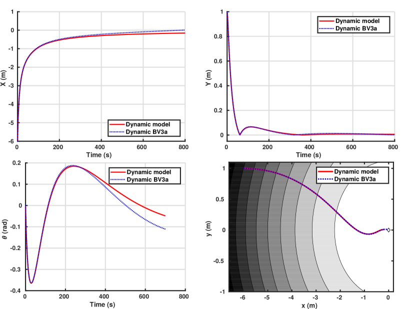
Figure 2: Simulation to evaluate the model accuracy with starting poses $x=-6$, $y=1$ and $\theta=0$

III-B Forward velocity increase towards the source

To illustrate the increase of the speed when the vehicle points towards the source – prediction from equation (9) – we simulated from the same initial position the standard Braitenberg vehicle 3a and our new model version, eq. (3). Specifically, the initial pose in both simulations was $x=-6$, $y=0$ and $\theta=0$, which leads to a straight line trajectory ($\dot{y}=0$ and $\dot{\theta}=0$) for our stimulus. Figure 3 shows the time evolution of the $x$ coordinate, which corresponds to the solution of equation (10). As we can see from the figure the version including the dynamics (with $\alpha=3$) approaches the origin faster than the standard Braitenberg vehicle 3a. We also concluded from the analysis of equation (9) that the forward speed in the dynamic version is reduced when the vehicle points away from the source. This effect will be shown in the next section together with the local stability of the trajectories around the straight line trajectory.

Figure 3: Trajectory over time of vehicles 3a and the proposed dynamic model with starting poses $x=-6$, $y=0$ and $\theta=0$

III-C Stability close to the analytical trajectory

As we saw in section II-B the real part of the eigenvalues of the linearised system can get more negative for the Braitenberg vehicle with the stimulus derivative controller. That means the convergence of trajectories towards the straight line solution is faster. To illustrate this effect we simulated the Braitenberg vehicle 3a with and without the dynamic contribution for a starting position close to the analytic straight line solution. Figure 4 shows the resulting trajectories with starting pose $x=-6$, $y=1$ and $\theta=0$. Since the stimulus is not circularly symmetric, oscillations appear (see [21]), i.e. two eigenvalues are complex conjugates, but the amplitude of the oscillations is smaller for the dynamic version due to the exponential term (real part of the eigenvalues) multiplying the oscillatory functions. The plot also shows that the trajectory of the dynamic version of the vehicle is shorter and seems to oscillate less around the linearisation trajectory, which seems to indicate that the imaginary part of the eigenvalues is also smaller.

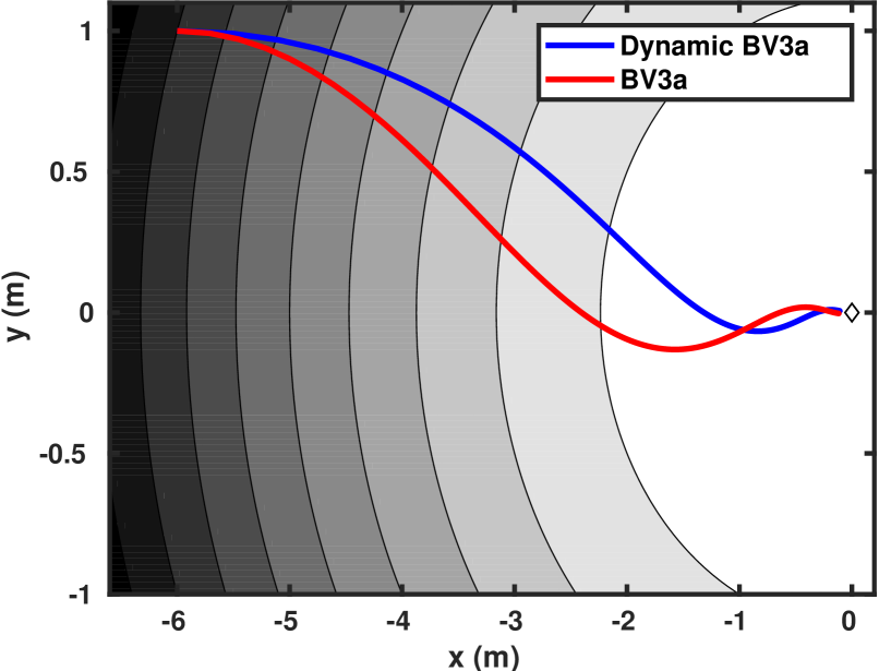
Figure 4: Simulation of the standard Braitenberg vehicle 3a with and without dynamic component with starting poses $x=-6$, $y=1$ and $\theta=0$

Finally, we ran a simulation to illustrate the effect on the reduction of the forward speed when the vehicle points in the opposite direction to the source, i.e. when $\nabla S^{T}\hat{e}<0$. According to equations (9) the speed should decrease compared to the standard vehicle 3a while the vehicle moves opposite to the source. Once it heads the direction of the gradient within $\pm\frac{\pi}{2}$ radians the forward speed increases. Figure 5 illustrates this effect by showing the trajectories of the vehicles starting with pose $x=-2$, $y=1$ and $\theta=\arctan-\frac{1}{2}$, i.e. pointing directly away from the source. As we can see the movement of the vehicle greatly improves when the controller includes the time derivative of the stimulus leading to a sharper turn and a shorter trajectory. Although in this case the initial pose of the vehicle is not close to the straight line trajectory, the vehicle firts turns towards the source and the approaches the horizontal axis where the equations of the linearised system are valid.

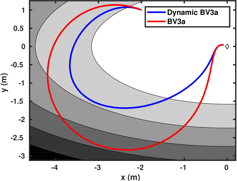
Figure 5: Simulation of the standard Braitenberg vehicle 3a with and without dynamic component with starting poses $x=-2$, $y=1$ and $\theta=\arctan-\frac{1}{2}$

IV Conclusions and Future Work

This paper proposes a new bio-inspired local navigation strategy that extends the well known Braitenberg models of animal positive taxes, while accounting for the experimental findings in biology showing that animals use the time evolution of the perceived stimulus to control their movement. We analysed the mathematical model of the dynamic Braitenberg vehicle and showed that the convergence towards the stimulus source is faster. This work has important implications in robotics as it shows the improvement control techniques based on optical flow or event based cameras – when the perception is dependent on the speed of the robot – can bring. Although the circular dependency between the controlled variables and the perceived variables makes the closed-loop system difficult to analyse, our simplified setup enables applying analytical tools to show that there is a clear improvement in the stability of the system.

One underlying assumptions to make the closed-loop system tractable is the absence of sensor noise or a high signal to noise ratio. However, biological systems are inherently noisy, and the time derivative of a perceptual signal with additive noise cannot be used directly to control a robot motion. It would require instead a band-pass filter. Therefore, our next step will focus on trying to analyse the behaviour of this new controller using a stochastic model of Braitenberg vehicles [23].

References

- [1] V. Braitenberg, Vehicles. Experiments in synthetic psychology. The MIT Press, 1984.
- [2] I. Rañó, “Biologically inspired navigation primitives,” Robot. and Auto. Sys., vol. 62, no. 10, pp. 1361–1370, 2014.
- [3] G. Fraenkel and D. Gunn, The orientation of animals. Kineses, taxes and compass reactions. Dover publications, 1961.
- [4] M. Hellwig and H. Tichy, “Rising background odor concentration reduces sensitivity of on and off olfactory receptor neurons for changes in concentration,” Frontiers in Phychology, vol. 7, pp. 1–7, 2016.
- [5] M. Bernard, S. N’Guyen, P. Pirim, B. Gas, and J.-A. Meyer, “Phonotaxis behavior in the artificial rat psikharpax,” in International Symposium on Robotics and Intelligent Sensors, IRIS2010, 2010.
- [6] D. Shaikh, J. Hallam, J. Christensen-Dalsgaard, and L. Zhang, “A Braitenberg lizard: Continuous phonotaxis with a lizard ear model,” in Proceedings of the 3rd Intl. Work-Conference on The Interplay Between Natural and Artificial Computation, 2009, pp. 439–448.
- [7] D. Shaikh, J. Hallam, and J. Christensen-Dalsgaard, “From “ear” to there: A review of biorobotic models of auditory processing in lizards,” Biological Cybernetics, vol. 110, no. 4-5, pp. 303–317, 2016.
- [8] B. Webb, A Spiking Neuron Controller for Robot Phonotaxis. The MIT/AAAI Press, 2001, pp. 3–20.
- [9] A. Horchler, R. Reeve, B. Webb, and R. Quinn, “Robot phonotaxis in the wild: a biologically inspired approach to outdoor sound localization,” Advanced Robotics, vol. 18, no. 8, pp. 801–816, 2004.
- [10] R. Reeve, B. Webb, A. Horchlerb, G. Indiveri, and R. Quinn, “New technologies for testing a model of cricket phonotaxis on an outdoor robot,” Robot. and Auton. Sys., vol. 51, no. 1, pp. 41–54, 2005.
- [11] A. J. Lilienthal and T. Duckett, “Experimental analysis of gas-sensitive Braitenberg vehicles,” Adv. Robot., vol. 18, no. 8, pp. 817–834, 2004.
- [12] T. Salumäe, I. Rañó, O. Akanyeti, and M. Kruusmaa, “Against the flow: A braitenberg controller for a fish robot,” in Proc. of the Intl. Conf. on Robot. and Autom., 2012, pp. 4210–4215.
- [13] V. Lebastard, F. Boyer, C. Chevallereau, and N. Servagent, “Underwater electro-naviagation in the dark,” in Proceedings of the International Conference on Robotics and Automation, 2012, pp. 1155–1160.
- [14] I. Rañó, A. Gómez-Eguíluz, and F. Sanfilippo, “Bridging the gap between bio-inspired steering and locomotion: A braitenberg 3a snake robot,” in Proceedingsd of the 15th International Conference on Control, Automation, Robotics and Vision, 2018.
- [15] M. Milde, H. Blum, A. Dietmüller, D. Sumislawska, J. Conradt, G. Indiveri, and Y. Sandamirskaya, “Obstacle avoidance and target aquisition for robot navigation using a mixed signal analog/digital neuromorphic processing system,” Front. in Neurorobot., vol. 24, 2017.
- [16] E. Bicho and G. Schöner, “The dynamic approach to autonomous robotics demonstrated on a low-level vehicle platform,” Robotics and Autonomous Systems, vol. 21, pp. 23–35, 1997.
- [17] I. Rañó, “The bio-inspired chaotic robot,” in Proc. of the IEEE Intl. Conf. on Robotics and Automation, 2014, pp. 304–309.
- [18] I. Rañó and J. Santos, “A biologically inspired controller to solve the coverage problem in robotics,” Bioinspiration & biomimetics, vol. 12, no. 3, 2017.
- [19] A. Pequeño, “A bioinspired neural control system based upon the cockroach active sensing antennae,” Master’s thesis, University of Southern Denmark, Denmark, 2018.
- [20] I. Rañó, “A steering taxis model and the qualitative analysis of its trajectories,” Adaptive Behavior, vol. 17, no. 3, pp. 197–211, 2009.
- [21] ——, “Results on the convergence of braitenberg vehicle 3a,” Artificial Life, vol. 20, no. 2, pp. 223–235, 2014.
- [22] L. Shampine, “Solving in matlab,” Journal of Numerical Mathematics, vol. 10, no. 4, pp. 291–310, 2002.
- [23] I. Rañó, M. Khamassi, and K. Wong-Lin, “A drift diffusion model of biological source seeking for mobile robots,” in Proceedings of the 2017 IEEE Intl. Conf. on Robot. and Autom., 2017, pp. 3525–3531.