OCU-PHYS 498

NITEP 9

March, 2019

Generalized cut operation

associated with higher order variation in tensor models

H. Itoyama^a,b,c and R. Yoshioka^c

^aNambu Yoichiro Institute of Theoretical and Experimental Physics (NITEP),
Osaka City University

^bDepartment of Mathematics and Physics, Graduate School of Science,
Osaka City University

^cOsaka City University Advanced Mathematical Institute (OCAMI)

3-3-138, Sugimoto, Sumiyoshi-ku, Osaka, 558-8585, Japan

Abstract

The cut and join operations play important roles in tensor models in general. We introduce a generalization of the cut operation associated with the higher order variations and demonstrate how they generate operators in the Aristotelian tensor model. We point out that, by successive choices of appropriate variations, the cut operation generalized this way can generate those operators which do not appear in the ring of the join operation, providing a tool to enumerate the operators by a level by level analysis recursively. We present a set of rules that control the emergence of such operators.

1 Introduction

The tensor model has a long history of its research [1, 2, 3, 4, 5, 6]. Recent interest has come from an intersection of thoughts on holography and randomness which are realized by several phenomena in quantum gravity in lower dimensions [7, 8, 9, 10, 11, 12, 13, 14, 15, 16, 17, 18, 19, 20, 21, 22, 23, 24, 25, 26]. Some of the insights come from the Virasoro structure of the matrix models [27, 28, 29, 30, 31, 32, 33, 34] and its combinatorics and finding its counterpart in tensor models in general is expected to pave the way to bring progress in this field. Recent references include [35, 36, 37, 38, 39, 40, 41, 42, 43, 44, 45, 46, 47, 48].

The Virasoro algebra has a natural extension named $w_{1+\infty}$ algebra whose roles at the 2-dimensional gravity and some integrable models have been well investigated. In particular, the constraints of $w_{1+\infty}$ type coming from the higher order contribution of the variation [31] have turned out to be algebraically independent and nontrivial in some of the matrix models such as the two-matrix model. Here we would like to discuss such higher order contributions arising from the change of the integration measure under the variation.

The basic structure of the contributions from the action is the join operation defined by

$$\{K,K^{\prime}\}=\frac{\partial K}{\partial A_{a_{1}a_{2}\cdots a_{r}}}\frac{\partial K^{\prime}}{\partial\bar{A}^{a_{1}a_{2}\cdots a_{r}}},$$ (1.1)

where $K$ and $K^{\prime}$ are arbitrary operators and the summation over the repeated indices is implied. When we choose appropriate keystone operators for $K$ and $K^{\prime}$, a block of independent operators called join pyramid is successively generated by the join operation. In other words, the join operation forms a ring whose elements are independent operators and the multiplication is given by (1.1). There are, however, operators which are not involved in the join pyramid and these can not be ignored because the cut operation which underlies the contribution from the variation of the integration measure generates these. These pieces of structure were discovered in [24]. (In contrast, the cut and join operation in one matrix model, namely, $r=2$, is depicted as going up and down at integer points on one-dimensional half-line.) The cut operation is defined by

$$\Delta K=\frac{\partial^{2}K}{\partial A_{a_{1}a_{2}\cdots a_{r}}\partial\bar{A}^{a_{1}a_{2}\cdots a_{r}}},$$ (1.2)

and corresponds to going up one stair (by one level) in the join pyramid. There is no systematic way to predict when a new operator appears and, in the situation of [24], one can try to discover this by acting the cut operation on all operators in the join pyramid only.

Taking the above mentioned role of the cut and join operation into account, we expect that the cut operation plays an important role in resolving the enumeration problem of the operators in tensor models. Below we will investigate higher order contributions to the constraints from the variation of the integral measure.

This paper is organized as follows: In section 2, the higher order variations of the integration measure are considered. In section 3, we discuss the successive choices of the variations. In section 4, we check that our choice of the variation is correct up to the level 6 operators. In section 5, a procedure of generating the operators not included in the join pyramid is described.

We owe most of our terminology to those seen in [22, 23, 24].

2 Higher order variation

Let us consider the rank $r=3$ Aristotelian tensor model. Let $A$ be a rank 3 tensor with its component $A_{\color[rgb]{1,0,0}{a_{1}}\color[rgb]{0,1,0}{a_{2}}\color[rgb]{0,0,1}{a_{3}}}$ and be its conjugate $\bar{A}$ with $\bar{A}^{\color[rgb]{1,0,0}{a_{1}}\color[rgb]{0,1,0}{a_{2}}\color[rgb]{0,0,1}{a_{3}}}$. Each index $a_{i}$, $i=1,2,3$ runs over $1,\cdots,N_{i}$ and is colored respectively in red, green and blue. The shift of integration variables of the partition function is defined by $A\to A+\delta A$ and $\bar{A}\to\bar{A}+\delta\bar{A}$ with

$$\delta A_{\color[rgb]{1,0,0}{a_{1}}\color[rgb]{0,1,0}{a_{2}}\color[rgb]{0,0,1}{a_{3}}}=\frac{\partial K}{\partial\bar{A}^{\color[rgb]{1,0,0}{a_{1}}\color[rgb]{0,1,0}{a_{2}}\color[rgb]{0,0,1}{a_{3}}}},~{}~{}~{}~{}~{}~{}~{}~{}~{}\delta\bar{A}^{\color[rgb]{1,0,0}{a_{1}}\color[rgb]{0,1,0}{a_{2}}\color[rgb]{0,0,1}{a_{3}}}=\frac{\partial K}{\partial{A}_{\color[rgb]{1,0,0}{a_{1}}\color[rgb]{0,1,0}{a_{2}}\color[rgb]{0,0,1}{a_{3}}}},$$ (2.1)

for arbitrary $K$. As the line element is given by

$$\mathrm{d}s^{2}_{A}=\sum_{\color[rgb]{1,0,0}{a_{1}},\color[rgb]{0,1,0}{a_{2}},\color[rgb]{0,0,1}{a_{3}}}\mathrm{d}A_{\color[rgb]{1,0,0}{a_{1}}\color[rgb]{0,1,0}{a_{2}}\color[rgb]{0,0,1}{a_{3}}}\mathrm{d}\bar{A}^{\color[rgb]{1,0,0}{a_{1}}\color[rgb]{0,1,0}{a_{2}}\color[rgb]{0,0,1}{a_{3}}}=\frac{1}{2}\begin{pmatrix}\mathrm{d}\bar{A}&\mathrm{d}A\end{pmatrix}\begin{pmatrix}\mathrm{d}A\\ \mathrm{d}\bar{A}\end{pmatrix},$$ (2.2)

its response under (2.1) is

$$\mathrm{d}s^{2}_{A+\delta A}=\begin{pmatrix}\mathrm{d}\bar{A}&\mathrm{d}A\end{pmatrix}(1+F)^{2}\begin{pmatrix}\mathrm{d}A\\ \mathrm{d}\bar{A}\end{pmatrix},$$ (2.3)

where the matrix $F$ of size $(2N_{1}N_{2}N_{3})\times(2N_{1}N_{2}N_{3})$ is defined by

$$F=\begin{pmatrix}\partial\bar{\partial}K&\bar{\partial}\bar{\partial}K\\ \partial\partial K&{\partial}\bar{\partial}K\end{pmatrix},~{}~{}~{}~{}~{}~{}~{}~{}\partial=\frac{\partial}{\partial A},~{}~{}~{}~{}~{}\bar{\partial}=\frac{\partial}{\partial\bar{A}}.$$ (2.4)

The measure is, therefore, transformed as

$$[\mathrm{d}A][\mathrm{d}\bar{A}]~{}~{}\longrightarrow~{}~{}\det(1+F)[\mathrm{d}A][\mathrm{d}\bar{A}],$$ (2.5)

where

$$\det(1+F)=1+\sum_{n=1}^{\infty}\frac{(-1)^{n}}{n}\mathrm{tr}F^{n}+\frac{1}{2}\sum_{n,m}\frac{(-1)^{n+m}}{nm}\mathrm{tr}F^{n}\mathrm{tr}F^{m}+\cdots.$$ (2.6)

The cut operator $\Delta$ (1.2) corresponds to

$$\mathrm{tr}F=2\Delta K.$$ (2.7)

We are interested in the higher order contribution at the response of the measure under the general variation and the gauge-invariant operators which are contained in $\det(1+F)$. We use the pictorial representation of the operators as follows: The tensor $A$ (resp. $\bar{A}$) are denoted by a white circle (resp. a black dot) and the contractions of indices are denoted by colored lines connecting between the white circles and the black dots. For example,

$$K_{1}\equiv A_{{\color[rgb]{1,0,0}a_{1}}{\color[rgb]{0,1,0}a_{2}}{\color[rgb]{0,0,1}a_{3}}}\bar{A}^{{\color[rgb]{1,0,0}a_{1}}{\color[rgb]{0,1,0}a_{2}}{\color[rgb]{0,0,1}a_{3}}}=\begin{picture}(14.0,7.0) \put(2.0,1.0){\color[rgb]{0,0,1}\line(1,0){10.0}} \put(-8.0,5.0){{\color[rgb]{1,0,0}\qbezier(10.0,-4.0)(15.0,0.0)(20.0,-4.0)}} \put(-8.0,5.0){{\color[rgb]{0,1,0}\qbezier(10.0,-4.0)(15.0,-8.0)(20.0,-4.0)}} \put(2.0,1.0){\circle{2.0}} \put(12.0,1.0){\circle*{2.0}} \put(0.0,-4.0){\mbox{$A$}} \put(11.0,-4.0){\mbox{$\bar{A}$}} \end{picture}$$ (2.8)

The connected operators come from $\mathrm{tr}F^{n}$. The number of $A$ in the operator under consideration is called level of the operator. In the case of $n=2$ and higher, the generalized cut operation $\mathrm{tr}F^{n}$ raises the level and therefore it can be used as the procedure which generates the higher level operators, while the usual cut operation (1.2) lowers the level of the operators by one. In the next section, we see that all connected operators at each level are included in $\mathrm{tr}F^{n}$ if $K$ is appropriately chosen.

3 Choice of $K$

In this section, we seek for the appropriate choice of the variation $K$ to construct all operators. Now let us choose temporarily

$$K_{\leq 2}=K_{\color[rgb]{1,0,0}{2}}+K_{\color[rgb]{0,1,0}{2}}+K_{\color[rgb]{0,0,1}{2}},$$ (3.1)

where

$$K_{\color[rgb]{1,0,0}{2}}=A_{\color[rgb]{1,0,0}{a_{1}}\color[rgb]{0,1,0}{a_{2}}\color[rgb]{0,0,1}{a_{3}}}A_{\color[rgb]{1,0,0}{a^{\prime}_{1}}\color[rgb]{0,1,0}{a^{\prime}_{2}}\color[rgb]{0,0,1}{a^{\prime}_{3}}}\bar{A}^{\color[rgb]{1,0,0}{a_{1}}\color[rgb]{0,1,0}{a^{\prime}_{2}}\color[rgb]{0,0,1}{a^{\prime}_{3}}}\bar{A}^{\color[rgb]{1,0,0}{a^{\prime}_{1}}\color[rgb]{0,1,0}{a_{2}}\color[rgb]{0,0,1}{a_{3}}}=\begin{picture}(20.0,10.0) \put(0.0,10.0){{\color[rgb]{0,1,0}\qbezier(6.0,-4.0)(13.0,0.0)(20.0,-4.0)}} \put(0.0,10.0){{\color[rgb]{0,0,1}\qbezier(6.0,-4.0)(13.0,-8.0)(20.0,-4.0)}} \put(6.0,-4.0){\color[rgb]{1,0,0}\line(0,1){10.0}} \put(20.0,-4.0){\color[rgb]{1,0,0}\line(0,1){10.0}} \put(6.0,6.0){\circle{2.0}} \put(20.0,6.0){\circle*{2.0}} \put(0.0,0.0){{\color[rgb]{0,1,0}\qbezier(6.0,-4.0)(13.0,0.0)(20.0,-4.0)}} \put(0.0,0.0){{\color[rgb]{0,0,1}\qbezier(6.0,-4.0)(13.0,-8.0)(20.0,-4.0)}} \put(6.0,-4.0){\circle*{2.0}} \put(20.0,-4.0){\circle{2.0}} \end{picture}~{}~{}.$$ (3.2)

The operator (3.1) is the linear combination of the level 2 operators and all operators in $\mathrm{tr}F^{n}$ are level $k=n$. Although $\mathrm{tr}F^{n}$ consists of $\partial\bar{\partial}K_{\leq 2}$ , $\partial\partial K_{\leq 2}$ and $\bar{\partial}\bar{\partial}K_{\leq 2}$, it turns out that only $\partial\bar{\partial}K_{\leq 2}$ is necessary below. Pictorially,

$$\partial\bar{\partial}K_{{\color[rgb]{1,0,0}2}}=2(A_{\color[rgb]{1,0,0}{a}\color[rgb]{0,1,0}{a_{2}}\color[rgb]{0,0,1}{a_{3}}}\bar{A}^{\color[rgb]{1,0,0}{a}\color[rgb]{0,1,0}{\bar{a}_{2}}\color[rgb]{0,0,1}{\bar{a}_{3}}}\delta_{\color[rgb]{1,0,0}{a_{1}}}^{\color[rgb]{1,0,0}{\bar{a}_{1}}}+A_{\color[rgb]{1,0,0}{a_{1}}\color[rgb]{0,1,0}{a}\color[rgb]{0,0,1}{b}}\bar{A}^{\color[rgb]{1,0,0}{\bar{a}_{1}}\color[rgb]{0,1,0}{a}\color[rgb]{0,0,1}{b}}\delta_{\color[rgb]{0,1,0}{a_{2}}}^{\color[rgb]{0,1,0}{\bar{a}_{2}}}\delta_{\color[rgb]{0,0,1}{a_{3}}}^{\color[rgb]{0,0,1}{\bar{a}_{3}}})\equiv 2\biggl{\{}({\color[rgb]{1,0,0}2})+({\color[rgb]{1,0,0}2})^{\prime}\biggl{\}},$$ (3.3)

$$\partial\bar{\partial}K_{{\color[rgb]{0,1,0}2}}=2(A_{\color[rgb]{1,0,0}{a_{1}}\color[rgb]{0,1,0}{a}\color[rgb]{0,0,1}{a_{3}}}\bar{A}^{\color[rgb]{1,0,0}{\bar{a}_{1}}\color[rgb]{0,1,0}{{a}}\color[rgb]{0,0,1}{\bar{a}_{3}}}\delta_{\color[rgb]{0,1,0}{a_{2}}}^{\color[rgb]{0,1,0}{\bar{a}_{2}}}+A_{\color[rgb]{1,0,0}{b}\color[rgb]{0,1,0}{a_{2}}\color[rgb]{0,0,1}{a}}\bar{A}^{\color[rgb]{1,0,0}{{b}}\color[rgb]{0,1,0}{\bar{a}_{2}}\color[rgb]{0,0,1}{a}}\delta_{\color[rgb]{1,0,0}{a_{1}}}^{\color[rgb]{1,0,0}{\bar{a}_{1}}}\delta_{\color[rgb]{0,0,1}{a_{3}}}^{\color[rgb]{0,0,1}{\bar{a}_{3}}})\equiv 2\biggl{\{}({\color[rgb]{0,1,0}2})+({\color[rgb]{0,1,0}2})^{\prime}\biggl{\}},$$ (3.4)

$$\partial\bar{\partial}K_{{\color[rgb]{0,0,1}2}}=2(A_{\color[rgb]{1,0,0}{a_{1}}\color[rgb]{0,1,0}{a_{2}}\color[rgb]{0,0,1}{a}}\bar{A}^{\color[rgb]{1,0,0}{\bar{a}_{1}}\color[rgb]{0,1,0}{\bar{a}_{2}}\color[rgb]{0,0,1}{{a}}}\delta_{\color[rgb]{0,0,1}{a_{3}}}^{\color[rgb]{0,0,1}{\bar{a}_{3}}}+A_{\color[rgb]{1,0,0}{a}\color[rgb]{0,1,0}{b}\color[rgb]{0,0,1}{a_{3}}}\bar{A}^{\color[rgb]{1,0,0}{{a}}\color[rgb]{0,1,0}{b}\color[rgb]{0,0,1}{\bar{a_{3}}}}\delta_{\color[rgb]{1,0,0}{a_{1}}}^{\color[rgb]{1,0,0}{\bar{a}_{1}}}\delta_{\color[rgb]{0,1,0}{a_{2}}}^{\color[rgb]{0,1,0}{\bar{a}_{2}}})\equiv 2\biggl{\{}({\color[rgb]{0,0,1}2})+({\color[rgb]{0,0,1}2})^{\prime}\biggl{\}},$$ (3.5)

where

$$({\color[rgb]{1,0,0}2})=~{}\begin{picture}(40.0,10.0) \put(5.0,6.0){\color[rgb]{1,0,0}\line(1,0){30.0}} \put(5.0,-4.0){\color[rgb]{0,1,0}\line(1,0){10.0}} \put(15.0,-4.0){\color[rgb]{1,0,0}\line(1,0){10.0}} \put(25.0,-4.0){\color[rgb]{0,1,0}\line(1,0){10.0}} \put(5.0,0.0){{\color[rgb]{0,0,1}\qbezier(0.0,1.0)(10.0,0.0)(10.0,-4.0)}} \put(5.0,0.0){{\color[rgb]{0,0,1}\qbezier(30.0,1.0)(20.0,0.0)(20.0,-4.0)}} \put(15.0,-4.0){\circle{2.0}} \put(25.0,-4.0){\circle*{2.0}} \put(13.0,-9.0){\mbox{$A$}} \put(23.0,-9.0){\mbox{$\bar{A}$}} \put(0.0,5.0){\mbox{$\color[rgb]{1,0,0}{a_{1}}$}} \put(0.0,0.0){\mbox{$\color[rgb]{0,0,1}{a_{3}}$}} \put(0.0,-5.0){\mbox{$\color[rgb]{0,1,0}{a_{2}}$}} \put(36.0,5.0){\mbox{$\color[rgb]{1,0,0}{a^{\prime}_{1}}$}} \put(36.0,0.0){\mbox{$\color[rgb]{0,0,1}{a^{\prime}_{3}}$}} \put(36.0,-5.0){\mbox{$\color[rgb]{0,1,0}{a^{\prime}_{2}}$}} \put(19.0,-3.0){\mbox{$\color[rgb]{1,0,0}a$}} \end{picture} ({\color[rgb]{1,0,0}2})^{\prime}=~{}\begin{picture}(40.0,10.0) \put(5.0,6.0){\color[rgb]{0,1,0}\line(1,0){30.0}} \put(5.0,1.0){\color[rgb]{0,0,1}\line(1,0){30.0}} \put(5.0,-4.0){\color[rgb]{1,0,0}\line(1,0){10.0}} \put(25.0,-4.0){\color[rgb]{1,0,0}\line(1,0){10.0}} \put(5.0,0.0){{\color[rgb]{0,1,0}\qbezier(10.0,-4.0)(15.0,0.0)(20.0,-4.0)}} \put(5.0,0.0){{\color[rgb]{0,0,1}\qbezier(10.0,-4.0)(15.0,-8.0)(20.0,-4.0)}} \put(15.0,-4.0){\circle{2.0}} \put(25.0,-4.0){\circle*{2.0}} \put(13.0,-9.0){\mbox{$A$}} \put(23.0,-9.0){\mbox{$\bar{A}$}} \put(0.0,5.0){\mbox{$\color[rgb]{0,1,0}{a_{2}}$}} \put(0.0,0.0){\mbox{$\color[rgb]{0,0,1}{a_{3}}$}} \put(0.0,-5.0){\mbox{$\color[rgb]{1,0,0}{a_{1}}$}} \put(36.0,5.0){\mbox{$\color[rgb]{0,1,0}{a^{\prime}_{2}}$}} \put(36.0,0.0){\mbox{$\color[rgb]{0,0,1}{a^{\prime}_{3}}$}} \put(36.0,-5.0){\mbox{$\color[rgb]{1,0,0}{a^{\prime}_{1}}$}} \put(19.0,-4.5){\mbox{$\color[rgb]{0,1,0}a$}} \put(19.0,-9.5){\mbox{$\color[rgb]{0,0,1}b$}} \end{picture}$$ (3.6)

$$({\color[rgb]{0,1,0}2})=~{}\begin{picture}(30.0,20.0) \put(5.0,6.0){\color[rgb]{0,1,0}\line(1,0){30.0}} \put(5.0,-4.0){\color[rgb]{0,0,1}\line(1,0){10.0}} \put(15.0,-4.0){\color[rgb]{0,1,0}\line(1,0){10.0}} \put(25.0,-4.0){\color[rgb]{0,0,1}\line(1,0){10.0}} \put(5.0,0.0){{\color[rgb]{1,0,0}\qbezier(0.0,1.0)(10.0,0.0)(10.0,-4.0)}} \put(5.0,0.0){{\color[rgb]{1,0,0}\qbezier(30.0,1.0)(20.0,0.0)(20.0,-4.0)}} \put(15.0,-4.0){\circle{2.0}} \put(25.0,-4.0){\circle*{2.0}} \put(13.0,-9.0){\mbox{$A$}} \put(23.0,-9.0){\mbox{$\bar{A}$}} \put(0.0,5.0){\mbox{$\color[rgb]{0,1,0}{a_{2}}$}} \put(0.0,0.0){\mbox{$\color[rgb]{1,0,0}{a_{1}}$}} \put(0.0,-5.0){\mbox{$\color[rgb]{0,0,1}{a_{3}}$}} \put(36.0,5.0){\mbox{$\color[rgb]{0,1,0}{a^{\prime}_{2}}$}} \put(36.0,0.0){\mbox{$\color[rgb]{1,0,0}{a^{\prime}_{1}}$}} \put(36.0,-5.0){\mbox{$\color[rgb]{0,0,1}{a^{\prime}_{3}}$}} \put(19.0,-3.0){\mbox{$\color[rgb]{0,1,0}a$}} \end{picture} ({\color[rgb]{0,1,0}2})^{\prime}=~{}\begin{picture}(40.0,20.0) \put(5.0,6.0){\color[rgb]{0,0,1}\line(1,0){30.0}} \put(5.0,1.0){\color[rgb]{1,0,0}\line(1,0){30.0}} \put(5.0,-4.0){\color[rgb]{0,1,0}\line(1,0){10.0}} \put(25.0,-4.0){\color[rgb]{0,1,0}\line(1,0){10.0}} \put(5.0,0.0){{\color[rgb]{0,0,1}\qbezier(10.0,-4.0)(15.0,0.0)(20.0,-4.0)}} \put(5.0,0.0){{\color[rgb]{1,0,0}\qbezier(10.0,-4.0)(15.0,-8.0)(20.0,-4.0)}} \put(15.0,-4.0){\circle{2.0}} \put(25.0,-4.0){\circle*{2.0}} \put(13.0,-9.0){\mbox{$A$}} \put(23.0,-9.0){\mbox{$\bar{A}$}} \put(0.0,5.0){\mbox{$\color[rgb]{0,0,1}{a_{3}}$}} \put(0.0,0.0){\mbox{$\color[rgb]{1,0,0}{a_{1}}$}} \put(0.0,-5.0){\mbox{$\color[rgb]{0,1,0}{a_{2}}$}} \put(36.0,5.0){\mbox{$\color[rgb]{0,0,1}{a^{\prime}_{3}}$}} \put(36.0,0.0){\mbox{$\color[rgb]{1,0,0}{a^{\prime}_{1}}$}} \put(36.0,-5.0){\mbox{$\color[rgb]{0,1,0}{a^{\prime}_{2}}$}} \put(19.0,-4.5){\mbox{$\color[rgb]{0,0,1}a$}} \put(19.0,-9.5){\mbox{$\color[rgb]{1,0,0}b$}} \end{picture}$$ (3.7)

$$({\color[rgb]{0,0,1}2})=~{}\begin{picture}(40.0,20.0) \put(5.0,6.0){\color[rgb]{0,0,1}\line(1,0){30.0}} \put(5.0,-4.0){\color[rgb]{1,0,0}\line(1,0){10.0}} \put(15.0,-4.0){\color[rgb]{0,0,1}\line(1,0){10.0}} \put(25.0,-4.0){\color[rgb]{1,0,0}\line(1,0){10.0}} \put(5.0,0.0){{\color[rgb]{0,1,0}\qbezier(0.0,1.0)(10.0,0.0)(10.0,-4.0)}} \put(5.0,0.0){{\color[rgb]{0,1,0}\qbezier(30.0,1.0)(20.0,0.0)(20.0,-4.0)}} \put(15.0,-4.0){\circle{2.0}} \put(25.0,-4.0){\circle*{2.0}} \put(13.0,-9.0){\mbox{$A$}} \put(23.0,-9.0){\mbox{$\bar{A}$}} \put(0.0,5.0){\mbox{$\color[rgb]{0,0,1}{a_{3}}$}} \put(0.0,0.0){\mbox{$\color[rgb]{0,1,0}{a_{2}}$}} \put(0.0,-5.0){\mbox{$\color[rgb]{1,0,0}{a_{1}}$}} \put(36.0,5.0){\mbox{$\color[rgb]{0,0,1}{a^{\prime}_{3}}$}} \put(36.0,0.0){\mbox{$\color[rgb]{0,1,0}{a^{\prime}_{2}}$}} \put(36.0,-5.0){\mbox{$\color[rgb]{1,0,0}{a^{\prime}_{1}}$}} \put(19.0,-3.0){\mbox{$\color[rgb]{0,0,1}a$}} \end{picture} ({\color[rgb]{0,0,1}2})^{\prime}=~{}\begin{picture}(40.0,20.0) \put(5.0,6.0){\color[rgb]{1,0,0}\line(1,0){30.0}} \put(5.0,1.0){\color[rgb]{0,1,0}\line(1,0){30.0}} \put(5.0,-4.0){\color[rgb]{0,0,1}\line(1,0){10.0}} \put(25.0,-4.0){\color[rgb]{0,0,1}\line(1,0){10.0}} \put(5.0,0.0){{\color[rgb]{1,0,0}\qbezier(10.0,-4.0)(15.0,0.0)(20.0,-4.0)}} \put(5.0,0.0){{\color[rgb]{0,1,0}\qbezier(10.0,-4.0)(15.0,-8.0)(20.0,-4.0)}} \put(15.0,-4.0){\circle{2.0}} \put(25.0,-4.0){\circle*{2.0}} \put(13.0,-9.0){\mbox{$A$}} \put(23.0,-9.0){\mbox{$\bar{A}$}} \put(0.0,5.0){\mbox{$\color[rgb]{1,0,0}{a_{1}}$}} \put(0.0,0.0){\mbox{$\color[rgb]{0,1,0}{a_{2}}$}} \put(0.0,-5.0){\mbox{$\color[rgb]{0,0,1}{a_{3}}$}} \put(36.0,5.0){\mbox{$\color[rgb]{1,0,0}{a^{\prime}_{1}}$}} \put(36.0,0.0){\mbox{$\color[rgb]{0,1,0}{a^{\prime}_{2}}$}} \put(36.0,-5.0){\mbox{$\color[rgb]{0,0,1}{a^{\prime}_{3}}$}} \put(19.0,-4.5){\mbox{$\color[rgb]{1,0,0}a$}} \put(19.0,-9.5){\mbox{$\color[rgb]{0,1,0}b$}} \end{picture}$$ (3.8)

In the subsections in what follows, we will show that all operators at the first few levels denoted generically by $k$ are included in $\mathrm{tr}F^{n}$.

3.1 level $k=1$

The only connected operator is $K_{1}=A_{\color[rgb]{1,0,0}{a_{1}}\color[rgb]{0,1,0}{a_{2}}\color[rgb]{0,0,1}{a_{3}}}\bar{A}^{\color[rgb]{1,0,0}{a_{1}}\color[rgb]{0,1,0}{a_{2}}\color[rgb]{0,0,1}{a_{3}}}$. In the case of $n=1$, $\mathrm{tr}F$ is the cut operation itself as mentioned above and we have

$$\mathrm{tr}F=4(N_{1}+N_{2}+N_{3}+(N_{1}N_{2}+N_{2}N_{3}+N_{3}N_{1}))K_{1}.$$ (3.9)

Conversely, we can obtain $K_{1}$ as the form of, for example,

$$K_{1}=\frac{1}{N_{1}}\mathrm{Tr}({\color[rgb]{1,0,0}2}).$$ (3.10)

Here the trace “$\mathrm{Tr}$” denotes the contraction of all indices. In the pictorial representation, it corresponds to connecting the two open lines with the same color on the both sides.

3.2 level $k=2$

All connected operators are listed in the appendix A2 of [24]. Similarly to the case of level $k=1$, $\mathrm{tr}F^{2}$ contains

$$K_{\color[rgb]{1,0,0}{2}}=\frac{1}{N_{1}}\mathrm{Tr}({\color[rgb]{1,0,0}2})^{2}.$$ (3.11)

The operators $K_{\color[rgb]{0,1,0}{2}}$ and $K_{\color[rgb]{0,0,1}{2}}$ are also obtained in a similar way.

3.3 level $k=3$

All connected operators are listed in the appendix A3 of [24]. At $n=3$, $\mathrm{tr}F^{3}$ contains not only

$$K_{\color[rgb]{1,0,0}{3}}=\frac{1}{N_{1}}\mathrm{Tr}({\color[rgb]{1,0,0}2})^{3},$$ (3.12)

$$K_{\color[rgb]{1,0,0}{2}\color[rgb]{0,1,0}{2}}=\mathrm{Tr}({\color[rgb]{1,0,0}2})^{2}({\color[rgb]{0,0,1}2}),$$ (3.13)

but also

$$K_{3W} =\mathrm{Tr}({\color[rgb]{1,0,0}2})({\color[rgb]{0,1,0}2})({\color[rgb]{0,0,1}2})$$ (3.14)

$$=\mathrm{Tr}~{}\begin{picture}(120.0,10.0) \put(0.0,6.0){\color[rgb]{1,0,0}\line(1,0){20.0}} \put(0.0,-4.0){\color[rgb]{0,1,0}\line(1,0){10.0}} \put(10.0,-4.0){\color[rgb]{1,0,0}\line(1,0){10.0}} \put(20.0,-4.0){\color[rgb]{0,0,1}\line(1,0){20.0}} \put(0.0,0.0){{\color[rgb]{1,0,0}\qbezier(20.0,6.0)(30.0,1.0)(40.0,-4.0)}} \put(0.0,0.0){{\color[rgb]{0,0,1}\qbezier(0.0,1.0)(10.0,0.0)(10.0,-4.0)}} \put(0.0,0.0){{\color[rgb]{0,1,0}\qbezier(20.0,-4.0)(30.0,1.0)(40.0,6.0)}} \put(10.0,-4.0){\circle{2.0}} \put(20.0,-4.0){\circle*{2.0}} \put(40.0,6.0){\color[rgb]{0,1,0}\line(1,0){10.0}} \put(40.0,-4.0){\color[rgb]{0,1,0}\line(1,0){10.0}} \put(50.0,-4.0){\color[rgb]{1,0,0}\line(1,0){10.0}} {\color[rgb]{0,0,1}\qbezier(50.0,-4.0)(60.0,1.0)(70.0,6.0)} \put(40.0,-4.0){\circle{2.0}} \put(50.0,-4.0){\circle*{2.0}} \put(70.0,6.0){\color[rgb]{0,0,1}\line(1,0){20.0}} \put(60.0,-4.0){\color[rgb]{1,0,0}\line(1,0){10.0}} \put(70.0,-4.0){\color[rgb]{0,0,1}\line(1,0){10.0}} \put(80.0,-4.0){\color[rgb]{1,0,0}\line(1,0){10.0}} {\color[rgb]{0,1,0}\qbezier(50.0,6.0)(60.0,1.0)(70.0,-4.0)} \put(60.0,0.0){{\color[rgb]{0,1,0}\qbezier(30.0,1.0)(20.0,0.0)(20.0,-4.0)}} \put(70.0,-4.0){\circle{2.0}} \put(80.0,-4.0){\circle*{2.0}} \put(9.0,-9.0){1} \put(19.0,-9.0){$\bar{1}$} \put(39.0,-9.0){3} \put(49.0,-9.0){$\bar{2}$} \put(69.0,-9.0){2} \put(79.0,-9.0){$\bar{3}$} \end{picture}$$ (3.15)

$$=~{}~{}~{}~{}\begin{picture}(100.0,80.0) \put(-4.0,0.0){ {\color[rgb]{1,0,0}{\qbezier(20.0,34.0)(10.0,17.0)(0.0,0.0)} {\qbezier(20.0,-34.0)(40.0,-34.0)(60.0,-34.0)} {\qbezier(80.0,0.0)(70.0,17.0)(60.0,34.0)}}} \put(-4.0,0.0){ {\color[rgb]{0,1,0}{\qbezier(0.0,0.0)(10.0,-17.0)(20.0,-34.0)} {\qbezier(60.0,-34.0)(70.0,-17.0)(80.0,0.0)} {\qbezier(60.0,34.0)(40.0,34.0)(20.0,34.0)}}} \put(-4.0,0.0){ {\color[rgb]{0,0,1}{\qbezier(20.0,34.0)(40.0,0.0)(60.0,-34.0)} {\qbezier(0.0,0.0)(40.0,0.0)(80.0,0.0)} {\qbezier(20.0,-34.0)(40.0,0.0)(60.0,34.0)}}} \put(20.0,34.0){\circle{6.0}} \put(20.0,-34.0){\circle{6.0}} \put(80.0,0.0){\circle{6.0}} \put(0.0,0.0){\circle*{6.0}} \put(60.0,-34.0){\circle*{6.0}} \put(60.0,34.0){\circle*{6.0}} \put(5.0,34.0){1} \put(5.0,-39.0){2} \put(90.0,-5.0){3} \put(-15.0,-5.0){$\bar{1}$} \put(70.0,-39.0){$\bar{2}$} \put(70.0,34.0){$\bar{3}$} \end{picture}.$$ (3.16)

The last one $K_{3W}$ cannot be obtained by the join operation. Hereafter, and in [22, 23, 24] such operators are called secondary operators. In the original procedure of [22, 23, 24], we had to act the original cut operation (1.2) on all of the level $k=4$ operators in order to discover the secondary operator $K_{3W}$.

3.4 level $k=4$

The independent operators are listed in the appendix A4 of [24]. At $n=4$, $\mathrm{tr}F^{4}$ contains

$$K_{\color[rgb]{1,0,0}4}=\frac{1}{N_{1}}\mathrm{Tr}({\color[rgb]{1,0,0}2})^{4},$$ (3.17)

$$K_{{\color[rgb]{0,0,1}3}{\color[rgb]{0,1,0}2}}=\frac{1}{N_{1}}\mathrm{Tr}({\color[rgb]{1,0,0}2})^{3}({\color[rgb]{0,1,0}2})^{\prime},$$ (3.18)

$$K_{222}=\frac{1}{N_{1}}\mathrm{Tr}({\color[rgb]{1,0,0}2})^{2}({\color[rgb]{0,1,0}2})^{\prime}({\color[rgb]{0,0,1}2})^{\prime},$$ (3.19)

$$K_{{\color[rgb]{1,0,0}2}{\color[rgb]{0,1,0}2}{\color[rgb]{1,0,0}2}}=\frac{1}{N_{2}}\mathrm{Tr}({\color[rgb]{1,0,0}2})^{\prime}({\color[rgb]{0,1,0}2})({\color[rgb]{1,0,0}2})^{\prime}({\color[rgb]{0,1,0}2}),$$ (3.20)

$$K_{{\color[rgb]{1,0,0}2}{\color[rgb]{0,0,1}2}{\color[rgb]{0,1,0}2}}=\frac{1}{N_{3}}\mathrm{Tr}({\color[rgb]{1,0,0}2})^{\prime}({\color[rgb]{0,0,1}2})({\color[rgb]{0,1,0}2})^{\prime}({\color[rgb]{0,0,1}2}),$$ (3.21)

$$\checkmark~{}~{}~{}~{} K_{4C}=\mathrm{Tr}({\color[rgb]{1,0,0}2})({\color[rgb]{0,1,0}2})({\color[rgb]{1,0,0}2})({\color[rgb]{0,1,0}2}),$$ (3.22)

$$K_{{\color[rgb]{1,0,0}3}{\color[rgb]{1,0,0}1}W}=\mathrm{Tr}({\color[rgb]{1,0,0}2})^{2}({\color[rgb]{0,0,1}2})({\color[rgb]{0,1,0}2}),$$ (3.23)

$$\checkmark~{}~{}~{}~{} K_{{\color[rgb]{1,0,0}2}{\color[rgb]{1,0,0}2}W}=\mathrm{Tr}({\color[rgb]{1,0,0}2})({\color[rgb]{0,1,0}2})({\color[rgb]{1,0,0}2})({\color[rgb]{0,0,1}2}).$$ (3.24)

The two operators $K_{4C}$ and $K_{\color[rgb]{1,0,0}{22}W}$ denoted by $\checkmark$ are secondary operators. We adopt $\checkmark$ notation to indicate secondary.

3.5 level $k=5$

At level $k=5$, $K_{\rm XXV}$, $K_{\rm XXVI}$ and $K_{\rm XXVIII}$ are still missing even with the generalized cut operation of this paper by the choice (3.1). In order to resolve this, let us replace (3.1) by

$$K_{\leq 3}=K_{\color[rgb]{1,0,0}{2}}+K_{\color[rgb]{0,1,0}{2}}+K_{\color[rgb]{0,0,1}{2}}+K_{3W}.$$ (3.25)

In this case, we have, in addition,

$$\partial\bar{\partial}K_{3W}=3\biggl{\{}(3W)_{\color[rgb]{1,0,0}r}+(3W)_{\color[rgb]{0,1,0}g}+(3W)_{\color[rgb]{0,0,1}b}\biggl{\}},$$ (3.26)

where

$$(3W)_{\color[rgb]{1,0,0}r}=\begin{picture}(50.0,10.0) \put(0.0,6.0){\color[rgb]{1,0,0}\line(1,0){50.0}} \put(0.0,-4.0){\color[rgb]{0,1,0}\line(1,0){10.0}} \put(10.0,-4.0){\color[rgb]{1,0,0}\line(1,0){10.0}} \put(20.0,-4.0){\color[rgb]{0,1,0}\line(1,0){10.0}} \put(30.0,-4.0){\color[rgb]{1,0,0}\line(1,0){10.0}} \put(40.0,-4.0){\color[rgb]{0,1,0}\line(1,0){10.0}} \put(0.0,0.0){{\color[rgb]{0,0,1}\qbezier(0.0,1.0)(30.0,0.0)(30.0,-4.0)}} \put(0.0,0.0){{\color[rgb]{0,0,1}\qbezier(50.0,1.0)(20.0,0.0)(20.0,-4.0)}} \put(0.0,0.0){{\color[rgb]{0,0,1}\qbezier(10.0,-4.0)(25.0,-15.0)(40.0,-4.0)}} \put(10.0,-4.0){\circle{2.0}} \put(20.0,-4.0){\circle*{2.0}} \put(30.0,-4.0){\circle{2.0}} \put(40.0,-4.0){\circle*{2.0}} \end{picture}~{}~{}=~{}~{}\begin{picture}(50.0,10.0) \put(0.0,6.0){\color[rgb]{1,0,0}\line(1,0){50.0}} \put(0.0,-4.0){\color[rgb]{0,0,1}\line(1,0){10.0}} \put(10.0,-4.0){\color[rgb]{1,0,0}\line(1,0){10.0}} \put(20.0,-4.0){\color[rgb]{0,0,1}\line(1,0){10.0}} \put(30.0,-4.0){\color[rgb]{1,0,0}\line(1,0){10.0}} \put(40.0,-4.0){\color[rgb]{0,0,1}\line(1,0){10.0}} \put(0.0,0.0){{\color[rgb]{0,1,0}\qbezier(0.0,1.0)(30.0,0.0)(30.0,-4.0)}} \put(0.0,0.0){{\color[rgb]{0,1,0}\qbezier(50.0,1.0)(20.0,0.0)(20.0,-4.0)}} \put(0.0,0.0){{\color[rgb]{0,1,0}\qbezier(10.0,-4.0)(25.0,-15.0)(40.0,-4.0)}} \put(10.0,-4.0){\circle{2.0}} \put(20.0,-4.0){\circle*{2.0}} \put(30.0,-4.0){\circle{2.0}} \put(40.0,-4.0){\circle*{2.0}} \end{picture}~{}~{},~{}~{}$$ (3.27)

$$(3W)_{\color[rgb]{0,1,0}g}=\begin{picture}(50.0,20.0) \put(0.0,6.0){\color[rgb]{0,1,0}\line(1,0){50.0}} \put(0.0,-4.0){\color[rgb]{0,0,1}\line(1,0){10.0}} \put(10.0,-4.0){\color[rgb]{0,1,0}\line(1,0){10.0}} \put(20.0,-4.0){\color[rgb]{0,0,1}\line(1,0){10.0}} \put(30.0,-4.0){\color[rgb]{0,1,0}\line(1,0){10.0}} \put(40.0,-4.0){\color[rgb]{0,0,1}\line(1,0){10.0}} \put(0.0,0.0){{\color[rgb]{1,0,0}\qbezier(0.0,1.0)(30.0,0.0)(30.0,-4.0)}} \put(0.0,0.0){{\color[rgb]{1,0,0}\qbezier(50.0,1.0)(20.0,0.0)(20.0,-4.0)}} \put(0.0,0.0){{\color[rgb]{1,0,0}\qbezier(10.0,-4.0)(25.0,-15.0)(40.0,-4.0)}} \put(10.0,-4.0){\circle{2.0}} \put(20.0,-4.0){\circle*{2.0}} \put(30.0,-4.0){\circle{2.0}} \put(40.0,-4.0){\circle*{2.0}} \end{picture}~{}~{}=~{}~{}\begin{picture}(50.0,10.0) \put(0.0,6.0){\color[rgb]{0,1,0}\line(1,0){50.0}} \put(0.0,-4.0){\color[rgb]{1,0,0}\line(1,0){10.0}} \put(10.0,-4.0){\color[rgb]{0,1,0}\line(1,0){10.0}} \put(20.0,-4.0){\color[rgb]{1,0,0}\line(1,0){10.0}} \put(30.0,-4.0){\color[rgb]{0,1,0}\line(1,0){10.0}} \put(40.0,-4.0){\color[rgb]{1,0,0}\line(1,0){10.0}} \put(0.0,0.0){{\color[rgb]{0,0,1}\qbezier(0.0,1.0)(30.0,0.0)(30.0,-4.0)}} \put(0.0,0.0){{\color[rgb]{0,0,1}\qbezier(50.0,1.0)(20.0,0.0)(20.0,-4.0)}} \put(0.0,0.0){{\color[rgb]{0,0,1}\qbezier(10.0,-4.0)(25.0,-15.0)(40.0,-4.0)}} \put(10.0,-4.0){\circle{2.0}} \put(20.0,-4.0){\circle*{2.0}} \put(30.0,-4.0){\circle{2.0}} \put(40.0,-4.0){\circle*{2.0}} \end{picture}~{}~{},~{}~{}$$ (3.28)

$$(3W)_{\color[rgb]{0,0,1}b}=\begin{picture}(50.0,20.0) \put(0.0,6.0){\color[rgb]{0,0,1}\line(1,0){50.0}} \put(0.0,-4.0){\color[rgb]{1,0,0}\line(1,0){10.0}} \put(10.0,-4.0){\color[rgb]{0,0,1}\line(1,0){10.0}} \put(20.0,-4.0){\color[rgb]{1,0,0}\line(1,0){10.0}} \put(30.0,-4.0){\color[rgb]{0,0,1}\line(1,0){10.0}} \put(40.0,-4.0){\color[rgb]{1,0,0}\line(1,0){10.0}} \put(0.0,0.0){{\color[rgb]{0,1,0}\qbezier(0.0,1.0)(30.0,0.0)(30.0,-4.0)}} \put(0.0,0.0){{\color[rgb]{0,1,0}\qbezier(50.0,1.0)(20.0,0.0)(20.0,-4.0)}} \put(0.0,0.0){{\color[rgb]{0,1,0}\qbezier(10.0,-4.0)(25.0,-15.0)(40.0,-4.0)}} \put(10.0,-4.0){\circle{2.0}} \put(20.0,-4.0){\circle*{2.0}} \put(30.0,-4.0){\circle{2.0}} \put(40.0,-4.0){\circle*{2.0}} \end{picture}~{}~{}=~{}~{}\begin{picture}(50.0,10.0) \put(0.0,6.0){\color[rgb]{0,0,1}\line(1,0){50.0}} \put(0.0,-4.0){\color[rgb]{0,1,0}\line(1,0){10.0}} \put(10.0,-4.0){\color[rgb]{0,0,1}\line(1,0){10.0}} \put(20.0,-4.0){\color[rgb]{0,1,0}\line(1,0){10.0}} \put(30.0,-4.0){\color[rgb]{0,0,1}\line(1,0){10.0}} \put(40.0,-4.0){\color[rgb]{0,1,0}\line(1,0){10.0}} \put(0.0,0.0){{\color[rgb]{1,0,0}\qbezier(0.0,1.0)(30.0,0.0)(30.0,-4.0)}} \put(0.0,0.0){{\color[rgb]{1,0,0}\qbezier(50.0,1.0)(20.0,0.0)(20.0,-4.0)}} \put(0.0,0.0){{\color[rgb]{1,0,0}\qbezier(10.0,-4.0)(25.0,-15.0)(40.0,-4.0)}} \put(10.0,-4.0){\circle{2.0}} \put(20.0,-4.0){\circle*{2.0}} \put(30.0,-4.0){\circle{2.0}} \put(40.0,-4.0){\circle*{2.0}} \end{picture}~{}~{}.~{}~{}$$ (3.29)

The subscripts ${\color[rgb]{1,0,0}r(ed)}$, ${\color[rgb]{0,1,0}g(reen)}$ and ${\color[rgb]{0,0,1}b(lue)}$ denote the color which acts trivially. Eq. (3.25) is the linear combination of operators whose levels are greater than or equal to 2. The levels of the operators in $\mathrm{tr}F^{n}$ are not always equal to $n$ in such case. To be more specific, operators of level $k$ must be included in $\mathrm{tr}F^{n}$ for some $n\leq k$.

Then, one can observe

$$K_{\rm XXV}=\mathrm{Tr}(3W)_{\color[rgb]{1,0,0}r}^{2}({\color[rgb]{1,0,0}2})~{}~{}~{}\in\mathrm{tr}F^{3},$$ (3.30)

$$\checkmark~{}~{}~{}~{} K_{\rm XXVI}=\mathrm{Tr}(3W)_{\color[rgb]{1,0,0}r}({\color[rgb]{0,1,0}2})({\color[rgb]{1,0,0}2})({\color[rgb]{0,0,1}2})~{}~{}~{}\in\mathrm{tr}F^{4}.$$ (3.31)

In addition, $K_{\rm XIV}$ is the secondary operator,

$$\checkmark~{}~{}~{}~{} K_{\rm XIV}=\mathrm{Tr}({\color[rgb]{1,0,0}2})({\color[rgb]{0,0,1}2})({\color[rgb]{0,1,0}2})({\color[rgb]{1,0,0}2})({\color[rgb]{0,1,0}2})~{}~{}~{}\in\mathrm{tr}F^{5},$$ (3.32)

which we can generate in the generalized cut operation already with (3.1).

We now arrive at a conjecture: in order to predict all connected operators at the higher levels, all we need to do is to add the new secondary operator at each lower level to $K$ successively. Then all connected operators at a given level $k$ are included in $\mathrm{tr}F^{n}(^{\exists}n\leq k)$.

$$\text{secondary}=\{K_{3W},K_{4C},K_{{\color[rgb]{1,0,0}2}{\color[rgb]{1,0,0}2}W},\cdots\}$$ (3.33)

4 Examination at level 6

At level 5, $K_{4C}$ and $K_{{\color[rgb]{1,0,0}22}W}$ (also $K_{{\color[rgb]{0,1,0}22}W}$ and $K_{{\color[rgb]{0,0,1}22}W}$, of course) appear as the new secondary operators. Hence, we choose

$$K_{\leq 4}=K_{\color[rgb]{1,0,0}{2}}+K_{\color[rgb]{0,1,0}{2}}+K_{\color[rgb]{0,0,1}{2}}+K_{3W}+K_{4C}+K_{{\color[rgb]{1,0,0}22}W}+K_{{\color[rgb]{0,1,0}22}W}+K_{{\color[rgb]{0,0,1}22}W}.$$ (4.1)

We then have

$$\partial\bar{\partial}K_{4C}=4\biggl{\{}(4C)+(4C)_{\color[rgb]{1,0,0}r}+(4C)_{\color[rgb]{0,1,0}g}+(4C)_{\color[rgb]{0,0,1}b}\biggl{\}},$$ (4.2)

where

$$(4C)_{\color[rgb]{1,0,0}r}=\begin{picture}(30.0,20.0) \put(0.0,12.0){\color[rgb]{1,0,0}\line(1,0){30.0}} \put(0.0,-8.0){\color[rgb]{0,0,1}\line(1,0){10.0}} \put(10.0,-8.0){\color[rgb]{1,0,0}\line(1,0){10.0}} \put(20.0,-8.0){\color[rgb]{0,0,1}\line(1,0){10.0}} \put(10.0,0.0){\color[rgb]{1,0,0}\line(1,0){10.0}} \put(10.0,8.0){\color[rgb]{1,0,0}\line(1,0){10.0}} \put(10.0,-8.0){\color[rgb]{0,1,0}\line(0,1){8.0}} \put(20.0,-8.0){\color[rgb]{0,1,0}\line(0,1){8.0}} \put(10.0,0.0){\color[rgb]{0,0,1}\line(0,1){8.0}} \put(20.0,0.0){\color[rgb]{0,0,1}\line(0,1){8.0}} \put(10.0,8.0){\color[rgb]{0,1,0}\line(-1,0){10.0}} \put(20.0,8.0){\color[rgb]{0,1,0}\line(1,0){10.0}} \put(10.0,-8.0){\circle{2.0}} \put(20.0,-8.0){\circle*{2.0}} \put(10.0,0.0){\circle*{2.0}} \put(20.0,0.0){\circle{2.0}} \put(10.0,8.0){\circle{2.0}} \put(20.0,8.0){\circle*{2.0}} \end{picture}~{}~{},~{}~{}~{}(4C)_{\color[rgb]{0,1,0}g}=\begin{picture}(30.0,20.0) \put(0.0,12.0){\color[rgb]{0,1,0}\line(1,0){30.0}} \put(0.0,-8.0){\color[rgb]{1,0,0}\line(1,0){10.0}} \put(10.0,-8.0){\color[rgb]{0,1,0}\line(1,0){10.0}} \put(20.0,-8.0){\color[rgb]{1,0,0}\line(1,0){10.0}} \put(10.0,0.0){\color[rgb]{0,1,0}\line(1,0){10.0}} \put(10.0,8.0){\color[rgb]{0,1,0}\line(1,0){10.0}} \put(10.0,-8.0){\color[rgb]{0,0,1}\line(0,1){8.0}} \put(20.0,-8.0){\color[rgb]{0,0,1}\line(0,1){8.0}} \put(10.0,0.0){\color[rgb]{1,0,0}\line(0,1){8.0}} \put(20.0,0.0){\color[rgb]{1,0,0}\line(0,1){8.0}} \put(10.0,8.0){\color[rgb]{0,0,1}\line(-1,0){10.0}} \put(20.0,8.0){\color[rgb]{0,0,1}\line(1,0){10.0}} \put(10.0,-8.0){\circle{2.0}} \put(20.0,-8.0){\circle*{2.0}} \put(10.0,0.0){\circle*{2.0}} \put(20.0,0.0){\circle{2.0}} \put(10.0,8.0){\circle{2.0}} \put(20.0,8.0){\circle*{2.0}} \end{picture}~{}~{},~{}~{}~{}(4C)_{\color[rgb]{0,0,1}b}=\begin{picture}(30.0,20.0) \put(0.0,12.0){\color[rgb]{0,0,1}\line(1,0){30.0}} \put(0.0,-8.0){\color[rgb]{0,1,0}\line(1,0){10.0}} \put(10.0,-8.0){\color[rgb]{0,0,1}\line(1,0){10.0}} \put(20.0,-8.0){\color[rgb]{0,1,0}\line(1,0){10.0}} \put(10.0,0.0){\color[rgb]{0,0,1}\line(1,0){10.0}} \put(10.0,8.0){\color[rgb]{0,0,1}\line(1,0){10.0}} \put(10.0,-8.0){\color[rgb]{1,0,0}\line(0,1){8.0}} \put(20.0,-8.0){\color[rgb]{1,0,0}\line(0,1){8.0}} \put(10.0,0.0){\color[rgb]{0,1,0}\line(0,1){8.0}} \put(20.0,0.0){\color[rgb]{0,1,0}\line(0,1){8.0}} \put(10.0,8.0){\color[rgb]{1,0,0}\line(-1,0){10.0}} \put(20.0,8.0){\color[rgb]{1,0,0}\line(1,0){10.0}} \put(10.0,-8.0){\circle{2.0}} \put(20.0,-8.0){\circle*{2.0}} \put(10.0,0.0){\circle*{2.0}} \put(20.0,0.0){\circle{2.0}} \put(10.0,8.0){\circle{2.0}} \put(20.0,8.0){\circle*{2.0}} \end{picture}$$ (4.3)

$$(4C)=\begin{picture}(40.0,30.0) \put(0.0,-6.0){\color[rgb]{1,0,0}\line(1,0){10.0}} \put(10.0,-6.0){\color[rgb]{0,1,0}\line(1,0){10.0}} \put(20.0,-6.0){\color[rgb]{1,0,0}\line(1,0){10.0}} \put(10.0,-6.0){\color[rgb]{0,0,1}\line(0,1){12.0}} \put(30.0,-6.0){\color[rgb]{0,0,1}\line(0,1){12.0}} \put(10.0,6.0){\color[rgb]{1,0,0}\line(1,0){10.0}} \put(20.0,6.0){\color[rgb]{0,1,0}\line(1,0){10.0}} \put(30.0,6.0){\color[rgb]{1,0,0}\line(1,0){10.0}} \put(0.0,0.0){{\color[rgb]{0,0,1}\qbezier(20.0,6.0)(20.0,2.0)(0.0,2.0)}} \put(0.0,0.0){{\color[rgb]{0,0,1}\qbezier(40.0,-2.0)(20.0,-2.0)(20.0,-6.0)}} \put(0.0,0.0){{\color[rgb]{0,1,0}\qbezier(10.0,6.0)(10.0,10.0)(40.0,10.0)}} \put(0.0,0.0){{\color[rgb]{0,1,0}\qbezier(30.0,-6.0)(30.0,-10.0)(0.0,-10.0)}} \put(10.0,-6.0){\circle{2.0}} \put(20.0,-6.0){\circle*{2.0}} \put(30.0,-6.0){\circle{2.0}} \put(10.0,6.0){\circle*{2.0}} \put(20.0,6.0){\circle{2.0}} \put(30.0,6.0){\circle*{2.0}} \end{picture}~{}~{},~{}~{}$$ (4.4)

and

$$\partial\bar{\partial}K_{{\color[rgb]{1,0,0}2}{\color[rgb]{1,0,0}2}W}=4\biggl{\{}({\color[rgb]{1,0,0}22}W)+({\color[rgb]{1,0,0}22}W)_{\color[rgb]{1,0,0}r}+({\color[rgb]{1,0,0}22}W)_{\color[rgb]{0,1,0}g}+({\color[rgb]{1,0,0}22}W)_{\color[rgb]{0,0,1}b}\biggl{\}},$$ (4.5)

where

$$({\color[rgb]{1,0,0}22}W)_{\color[rgb]{1,0,0}r}=\begin{picture}(30.0,25.0) \put(0.0,12.0){\color[rgb]{1,0,0}\line(1,0){30.0}} \put(0.0,-8.0){\color[rgb]{0,0,1}\line(1,0){10.0}} \put(10.0,-8.0){\color[rgb]{1,0,0}\line(1,0){10.0}} \put(20.0,-8.0){\color[rgb]{0,1,0}\line(1,0){10.0}} \put(10.0,0.0){\color[rgb]{1,0,0}\line(1,0){10.0}} \put(10.0,8.0){\color[rgb]{1,0,0}\line(1,0){10.0}} \put(10.0,-8.0){\color[rgb]{0,1,0}\line(0,1){8.0}} \put(20.0,-8.0){\color[rgb]{0,0,1}\line(0,1){8.0}} \put(10.0,0.0){\color[rgb]{0,0,1}\line(0,1){8.0}} \put(20.0,0.0){\color[rgb]{0,1,0}\line(0,1){8.0}} \put(10.0,8.0){\color[rgb]{0,1,0}\line(-1,0){10.0}} \put(20.0,8.0){\color[rgb]{0,0,1}\line(1,0){10.0}} \put(10.0,-8.0){\circle{2.0}} \put(20.0,-8.0){\circle*{2.0}} \put(10.0,0.0){\circle*{2.0}} \put(20.0,0.0){\circle{2.0}} \put(10.0,8.0){\circle{2.0}} \put(20.0,8.0){\circle*{2.0}} \end{picture}~{}~{},~{}~{}~{}$$ (4.6)

$$({\color[rgb]{1,0,0}22}W)_{\color[rgb]{0,1,0}g}=\begin{picture}(30.0,25.0) \put(0.0,12.0){\color[rgb]{0,1,0}\line(1,0){30.0}} \put(0.0,-8.0){\color[rgb]{1,0,0}\line(1,0){10.0}} \put(10.0,-8.0){\color[rgb]{0,0,1}\line(1,0){10.0}} \put(20.0,-8.0){\color[rgb]{1,0,0}\line(1,0){10.0}} \put(10.0,0.0){\color[rgb]{0,0,1}\line(1,0){10.0}} \put(10.0,8.0){\color[rgb]{0,1,0}\line(1,0){10.0}} \put(10.0,-8.0){\color[rgb]{0,1,0}\line(0,1){8.0}} \put(20.0,-8.0){\color[rgb]{0,1,0}\line(0,1){8.0}} \put(10.0,0.0){\color[rgb]{1,0,0}\line(0,1){8.0}} \put(20.0,0.0){\color[rgb]{1,0,0}\line(0,1){8.0}} \put(10.0,8.0){\color[rgb]{0,0,1}\line(-1,0){10.0}} \put(20.0,8.0){\color[rgb]{0,0,1}\line(1,0){10.0}} \put(10.0,-8.0){\circle{2.0}} \put(20.0,-8.0){\circle*{2.0}} \put(10.0,0.0){\circle*{2.0}} \put(20.0,0.0){\circle{2.0}} \put(10.0,8.0){\circle{2.0}} \put(20.0,8.0){\circle*{2.0}} \end{picture}~{}~{},~{}~{}~{}~{}~{}~{}~{}({\color[rgb]{1,0,0}22}W)_{\color[rgb]{0,0,1}b}=\begin{picture}(30.0,25.0) \put(0.0,12.0){\color[rgb]{0,0,1}\line(1,0){30.0}} \put(0.0,-8.0){\color[rgb]{1,0,0}\line(1,0){10.0}} \put(10.0,-8.0){\color[rgb]{0,1,0}\line(1,0){10.0}} \put(20.0,-8.0){\color[rgb]{1,0,0}\line(1,0){10.0}} \put(10.0,0.0){\color[rgb]{0,1,0}\line(1,0){10.0}} \put(10.0,8.0){\color[rgb]{0,0,1}\line(1,0){10.0}} \put(10.0,-8.0){\color[rgb]{0,0,1}\line(0,1){8.0}} \put(20.0,-8.0){\color[rgb]{0,0,1}\line(0,1){8.0}} \put(10.0,0.0){\color[rgb]{1,0,0}\line(0,1){8.0}} \put(20.0,0.0){\color[rgb]{1,0,0}\line(0,1){8.0}} \put(10.0,8.0){\color[rgb]{0,1,0}\line(-1,0){10.0}} \put(20.0,8.0){\color[rgb]{0,1,0}\line(1,0){10.0}} \put(10.0,-8.0){\circle{2.0}} \put(20.0,-8.0){\circle*{2.0}} \put(10.0,0.0){\circle*{2.0}} \put(20.0,0.0){\circle{2.0}} \put(10.0,8.0){\circle{2.0}} \put(20.0,8.0){\circle*{2.0}} \end{picture}~{}~{},$$ (4.7)

$$({\color[rgb]{1,0,0}22}W)=\begin{picture}(40.0,30.0) \put(0.0,-6.0){\color[rgb]{1,0,0}\line(1,0){10.0}} \put(10.0,-6.0){\color[rgb]{0,1,0}\line(1,0){10.0}} \put(20.0,-6.0){\color[rgb]{1,0,0}\line(1,0){10.0}} \put(10.0,-6.0){\color[rgb]{0,0,1}\line(0,1){12.0}} \put(30.0,-6.0){\color[rgb]{0,1,0}\line(0,1){12.0}} \put(10.0,6.0){\color[rgb]{1,0,0}\line(1,0){10.0}} \put(20.0,6.0){\color[rgb]{0,0,1}\line(1,0){10.0}} \put(30.0,6.0){\color[rgb]{1,0,0}\line(1,0){10.0}} \put(0.0,0.0){{\color[rgb]{0,1,0}\qbezier(20.0,6.0)(20.0,2.0)(0.0,2.0)}} \put(0.0,0.0){{\color[rgb]{0,0,1}\qbezier(40.0,-2.0)(20.0,-2.0)(20.0,-6.0)}} \put(0.0,0.0){{\color[rgb]{0,1,0}\qbezier(10.0,6.0)(10.0,10.0)(40.0,10.0)}} \put(0.0,0.0){{\color[rgb]{0,0,1}\qbezier(30.0,-6.0)(30.0,-10.0)(0.0,-10.0)}} \put(10.0,-6.0){\circle{2.0}} \put(20.0,-6.0){\circle*{2.0}} \put(30.0,-6.0){\circle{2.0}} \put(10.0,6.0){\circle*{2.0}} \put(20.0,6.0){\circle{2.0}} \put(30.0,6.0){\circle*{2.0}} \end{picture}~{}~{}.~{}~{}$$ (4.8)

We checked by direct inspection that all operators at level 6 are included in $\mathrm{tr}F^{n}(^{\exists}n\leq 6)$ with $K_{\leq 4}$. We plan to elaborate upon this in the future. In particular, we found 10 independent secondary operators at level 6 up to the coloring,

$$\mathrm{Tr}({\color[rgb]{1,0,0}2})({\color[rgb]{0,1,0}2})({\color[rgb]{1,0,0}2})({\color[rgb]{0,1,0}2})({\color[rgb]{1,0,0}2})({\color[rgb]{0,1,0}2}) =~{}~{}~{}~{}~{}\begin{picture}(90.0,80.0) \put(-4.0,0.0){ {\color[rgb]{1,0,0}{\qbezier(20.0,34.0)(10.0,17.0)(0.0,0.0)} {\qbezier(20.0,-34.0)(40.0,-34.0)(60.0,-34.0)} {\qbezier(80.0,0.0)(70.0,17.0)(60.0,34.0)} {\qbezier(20.0,0.0)(25.0,8.5)(30.0,17.0)} {\qbezier(50.0,17.0)(55.0,8.5)(60.0,0.0)} {\qbezier(30.0,-17.0)(40.0,-17.0)(50.0,-17.0)} }} \put(-4.0,0.0){ {\color[rgb]{0,1,0}{\qbezier(0.0,0.0)(10.0,-17.0)(20.0,-34.0)} {\qbezier(60.0,-34.0)(70.0,-17.0)(80.0,0.0)} {\qbezier(60.0,34.0)(40.0,34.0)(20.0,34.0)} {\qbezier(20.0,0.0)(25.0,-8.5)(30.0,-17.0)} {\qbezier(50.0,-17.0)(55.0,-8.5)(60.0,0.0)} {\qbezier(30.0,17.0)(40.0,17.0)(50.0,17.0)} }} \put(-4.0,0.0){ {\color[rgb]{0,0,1}{\qbezier(20.0,34.0)(25.0,25.5)(30.0,17.0)} {\qbezier(0.0,0.0)(10.0,0.0)(20.0,0.0)} {\qbezier(50.0,17.0)(55.0,25.5)(60.0,34.0)} {\qbezier(60.0,0.0)(70.0,0.0)(80.0,0.0)} {\qbezier(50.0,-17.0)(55.0,-25.5)(60.0,-34.0)} {\qbezier(20.0,-34.0)(25.0,-25.5)(30.0,-17.0)} }} \put(20.0,34.0){\circle{6.0}} \put(20.0,-34.0){\circle{6.0}} \put(80.0,0.0){\circle{6.0}} \put(0.0,0.0){\circle*{6.0}} \put(60.0,-34.0){\circle*{6.0}} \put(60.0,34.0){\circle*{6.0}} \put(30.0,17.0){\circle*{6.0}} \put(50.0,17.0){\circle{6.0}} \put(60.0,0.0){\circle*{6.0}} \put(50.0,-17.0){\circle{6.0}} \put(30.0,-17.0){\circle*{6.0}} \put(20.0,0.0){\circle{6.0}} \end{picture},$$ (4.9)

$$\mathrm{Tr}({\color[rgb]{1,0,0}2})({\color[rgb]{0,1,0}2})({\color[rgb]{1,0,0}2})({\color[rgb]{0,1,0}2})({\color[rgb]{1,0,0}2})({\color[rgb]{0,0,1}2}) =~{}~{}~{}~{}~{}\begin{picture}(90.0,80.0) \put(-4.0,0.0){ {\color[rgb]{1,0,0}{\qbezier(0.0,10.0)(0.0,0.0)(0.0,-10.0)} {\qbezier(16.0,-24.0)(24.0,-31.0)(32.0,-38.0)} {\qbezier(52.0,-38.0)(60.0,-31.0)(68.0,-24.0)} {\qbezier(84.0,-10.0)(84.0,0.0)(84.0,10.0)} {\qbezier(68.0,24.0)(60.0,31.0)(52.0,38.0)} {\qbezier(32.0,38.0)(24.0,31.0)(16.0,24.0)} }} \put(-4.0,0.0){ {\color[rgb]{0,1,0}{\qbezier(0.0,10.0)(8.0,17.0)(16.0,24.0)} {\qbezier(32.0,38.0)(42.0,38.0)(52.0,38.0)} {\qbezier(68.0,24.0)(76.0,17.0)(84.0,10.0)} {\qbezier(0.0,-10.0)(8.0,-17.0)(16.0,-24.0)} {\qbezier(32.0,-38.0)(42.0,-38.0)(52.0,-38.0)} {\qbezier(68.0,-24.0)(76.0,-17.0)(84.0,-10.0)} }} \put(-4.0,0.0){ {\color[rgb]{0,0,1}{\qbezier(0.0,10.0)(42.0,10.0)(84.0,10.0)} {\qbezier(16.0,24.0)(42.0,24.0)(68.0,24.0)} {\qbezier(0.0,-10.0)(42.0,-10.0)(84.0,-10.0)} {\qbezier(16.0,-24.0)(42.0,-24.0)(68.0,-24.0)} {\qbezier(32.0,38.0)(32.0,0.0)(32.0,-38.0)} {\qbezier(52.0,38.0)(52.0,0.0)(52.0,-38.0)} }} \put(0.0,10.0){\circle{6.0}} \put(16.0,24.0){\circle*{6.0}} \put(32.0,38.0){\circle{6.0}} \put(52.0,38.0){\circle*{6.0}} \put(68.0,24.0){\circle{6.0}} \put(84.0,10.0){\circle*{6.0}} \put(0.0,-10.0){\circle*{6.0}} \put(16.0,-24.0){\circle{6.0}} \put(32.0,-38.0){\circle*{6.0}} \put(52.0,-38.0){\circle{6.0}} \put(68.0,-24.0){\circle*{6.0}} \put(84.0,-10.0){\circle{6.0}} \end{picture},$$ (4.10)

$$\mathrm{Tr}({\color[rgb]{1,0,0}2})({\color[rgb]{0,1,0}2})({\color[rgb]{1,0,0}2})({\color[rgb]{0,0,1}2})({\color[rgb]{0,1,0}2})({\color[rgb]{0,0,1}2}) =~{}~{}~{}~{}~{}~{}\begin{picture}(90.0,80.0) \put(-4.0,0.0){ {\color[rgb]{1,0,0}{\qbezier(0.0,14.0)(12.0,24.0)(24.0,34.0)} {\qbezier(52.0,34.0)(64.0,24.0)(76.0,14.0)} {\qbezier(24.0,10.0)(38.0,10.0)(52.0,10.0)} {\qbezier(0.0,-14.0)(12.0,-24.0)(24.0,-34.0)} {\qbezier(52.0,-34.0)(64.0,-24.0)(76.0,-14.0)} {\qbezier(24.0,-10.0)(38.0,-10.0)(52.0,-10.0)} }} \put(-4.0,0.0){ {\color[rgb]{0,1,0}{\qbezier(24.0,34.0)(38.0,34.0)(52.0,34.0)} {\qbezier(24.0,-34.0)(38.0,-34.0)(52.0,-34.0)} {\qbezier(0.0,14.0)(0.0,0.0)(0.0,-14.0)} {\qbezier(76.0,14.0)(76.0,0.0)(76.0,-14.0)} {\qbezier(24.0,10.0)(24.0,0.0)(24.0,-10.0)} {\qbezier(52.0,10.0)(52.0,0.0)(52.0,-10.0)} }} \put(-4.0,0.0){ {\color[rgb]{0,0,1}{\qbezier(24.0,34.0)(24.0,22.0)(24.0,10.0)} {\qbezier(52.0,34.0)(52.0,22.0)(52.0,10.0)} {\qbezier(24.0,-34.0)(24.0,-22.0)(24.0,-10.0)} {\qbezier(52.0,-34.0)(52.0,-22.0)(52.0,-10.0)} {\qbezier(0.0,14.0)(38.0,30.0)(76.0,14.0)} {\qbezier(0.0,-14.0)(38.0,-30.0)(76.0,-14.0)} }} \put(0.0,14.0){\circle*{6.0}} \put(24.0,34.0){\circle{6.0}} \put(52.0,34.0){\circle*{6.0}} \put(76.0,14.0){\circle{6.0}} \put(0.0,-14.0){\circle{6.0}} \put(24.0,-34.0){\circle*{6.0}} \put(52.0,-34.0){\circle{6.0}} \put(76.0,-14.0){\circle*{6.0}} \put(24.0,10.0){\circle*{6.0}} \put(52.0,10.0){\circle{6.0}} \put(24.0,-10.0){\circle{6.0}} \put(52.0,-10.0){\circle*{6.0}} \end{picture},$$ (4.11)

$$\mathrm{Tr}({\color[rgb]{1,0,0}2})({\color[rgb]{0,1,0}2})({\color[rgb]{0,0,1}2})({\color[rgb]{1,0,0}2})({\color[rgb]{0,1,0}2})({\color[rgb]{0,0,1}2}) =~{}~{}~{}~{}~{}\begin{picture}(90.0,80.0) \put(-4.0,0.0){ {\color[rgb]{1,0,0}{\qbezier(20.0,34.0)(10.0,17.0)(0.0,0.0)} {\qbezier(20.0,-34.0)(40.0,-34.0)(60.0,-34.0)} {\qbezier(80.0,0.0)(70.0,17.0)(60.0,34.0)} {\qbezier(20.0,0.0)(25.0,8.5)(30.0,17.0)} {\qbezier(50.0,17.0)(55.0,8.5)(60.0,0.0)} {\qbezier(30.0,-17.0)(40.0,-17.0)(50.0,-17.0)} }} \put(-4.0,0.0){ {\color[rgb]{0,1,0}{\qbezier(0.0,0.0)(10.0,-17.0)(20.0,-34.0)} {\qbezier(60.0,-34.0)(70.0,-17.0)(80.0,0.0)} {\qbezier(60.0,34.0)(40.0,34.0)(20.0,34.0)} {\qbezier(20.0,0.0)(25.0,-8.5)(30.0,-17.0)} {\qbezier(50.0,-17.0)(55.0,-8.5)(60.0,0.0)} {\qbezier(30.0,17.0)(40.0,17.0)(50.0,17.0)} }} \put(-4.0,0.0){ {\color[rgb]{0,0,1}{\qbezier(20.0,34.0)(25.0,25.5)(30.0,17.0)} {\qbezier(0.0,0.0)(40.0,60.0)(80.0,0.0)} {\qbezier(50.0,17.0)(55.0,25.5)(60.0,34.0)} {\qbezier(60.0,0.0)(40.0,0.0)(20.0,0.0)} {\qbezier(50.0,-17.0)(55.0,-25.5)(60.0,-34.0)} {\qbezier(20.0,-34.0)(25.0,-25.5)(30.0,-17.0)} }} \put(20.0,34.0){\circle{6.0}} \put(20.0,-34.0){\circle{6.0}} \put(80.0,0.0){\circle{6.0}} \put(0.0,0.0){\circle*{6.0}} \put(60.0,-34.0){\circle*{6.0}} \put(60.0,34.0){\circle*{6.0}} \put(30.0,17.0){\circle*{6.0}} \put(50.0,17.0){\circle{6.0}} \put(60.0,0.0){\circle*{6.0}} \put(50.0,-17.0){\circle{6.0}} \put(30.0,-17.0){\circle*{6.0}} \put(20.0,0.0){\circle{6.0}} \end{picture},$$ (4.12)

$$\mathrm{Tr}(3W)_{\color[rgb]{1,0,0}r}({\color[rgb]{0,1,0}2})({\color[rgb]{0,0,1}2})({\color[rgb]{0,1,0}2})({\color[rgb]{0,0,1}2}) =~{}~{}~{}~{}~{}~{}\begin{picture}(90.0,80.0) \put(-4.0,0.0){ {\color[rgb]{1,0,0}{\qbezier(0.0,14.0)(12.0,24.0)(24.0,34.0)} {\qbezier(52.0,34.0)(64.0,24.0)(76.0,14.0)} {\qbezier(0.0,-14.0)(12.0,-24.0)(24.0,-34.0)} {\qbezier(52.0,-34.0)(64.0,-24.0)(76.0,-14.0)} {\qbezier(30.0,0.0)(38.0,7.0)(46.0,14.0)} {\qbezier(46.0,-14.0)(54.0,-7.0)(62.0,0.0)} }} \put(-4.0,0.0){ {\color[rgb]{0,1,0}{\qbezier(24.0,34.0)(38.0,34.0)(52.0,34.0)} {\qbezier(24.0,-34.0)(38.0,-34.0)(52.0,-34.0)} {\qbezier(0.0,14.0)(0.0,0.0)(0.0,-14.0)} {\qbezier(76.0,14.0)(76.0,0.0)(76.0,-14.0)} {\qbezier(30.0,0.0)(46.0,0.0)(62.0,0.0)} {\qbezier(46.0,14.0)(46.0,0.0)(46.0,-14.0)} }} \put(-4.0,0.0){ {\color[rgb]{0,0,1}{\qbezier(0.0,14.0)(38.0,36.0)(76.0,14.0)} {\qbezier(24.0,34.0)(8.0,0.0)(24.0,-34.0)} {\qbezier(52.0,34.0)(49.0,24.0)(46.0,14.0)} {\qbezier(0.0,-14.0)(15.0,-7.0)(30.0,0.0)} {\qbezier(52.0,-34.0)(49.0,-24.0)(46.0,-14.0)} {\qbezier(76.0,-14.0)(69.0,-7.0)(62.0,0.0)} }} \put(0.0,14.0){\circle*{6.0}} \put(24.0,34.0){\circle{6.0}} \put(52.0,34.0){\circle*{6.0}} \put(76.0,14.0){\circle{6.0}} \put(0.0,-14.0){\circle{6.0}} \put(24.0,-34.0){\circle*{6.0}} \put(52.0,-34.0){\circle{6.0}} \put(76.0,-14.0){\circle*{6.0}} \put(46.0,14.0){\circle{6.0}} \put(30.0,0.0){\circle*{6.0}} \put(46.0,-14.0){\circle*{6.0}} \put(62.0,0.0){\circle{6.0}} \end{picture},$$ (4.13)

$$\mathrm{Tr}(3W)_{\color[rgb]{1,0,0}r}({\color[rgb]{0,1,0}2})({\color[rgb]{1,0,0}2})({\color[rgb]{0,1,0}2})({\color[rgb]{0,0,1}2}) =~{}~{}~{}~{}~{}\begin{picture}(90.0,80.0) \put(-4.0,0.0){ {\color[rgb]{1,0,0}{\qbezier(0.0,10.0)(0.0,0.0)(0.0,-10.0)} {\qbezier(16.0,-24.0)(24.0,-31.0)(32.0,-38.0)} {\qbezier(52.0,-38.0)(60.0,-31.0)(68.0,-24.0)} {\qbezier(84.0,-10.0)(84.0,0.0)(84.0,10.0)} {\qbezier(68.0,24.0)(60.0,31.0)(52.0,38.0)} {\qbezier(32.0,38.0)(24.0,31.0)(16.0,24.0)} }} \put(-4.0,0.0){ {\color[rgb]{0,1,0}{\qbezier(0.0,10.0)(8.0,17.0)(16.0,24.0)} {\qbezier(32.0,38.0)(42.0,38.0)(52.0,38.0)} {\qbezier(68.0,24.0)(76.0,17.0)(84.0,10.0)} {\qbezier(0.0,-10.0)(8.0,-17.0)(16.0,-24.0)} {\qbezier(32.0,-38.0)(42.0,-38.0)(52.0,-38.0)} {\qbezier(68.0,-24.0)(76.0,-17.0)(84.0,-10.0)} }} \put(-4.0,0.0){ {\color[rgb]{0,0,1}{\qbezier(0.0,10.0)(34.0,-7.0)(68.0,-24.0)} {\qbezier(16.0,24.0)(42.0,24.0)(68.0,24.0)} {\qbezier(32.0,38.0)(26.0,4.0)(0.0,-10.0)} {\qbezier(52.0,38.0)(52.0,0.0)(52.0,-38.0)} {\qbezier(84.0,10.0)(42.0,24.0)(16.0,-24.0)} {\qbezier(32.0,-38.0)(35.0,-5.0)(84.0,-10.0)} }} \put(0.0,10.0){\circle{6.0}} \put(16.0,24.0){\circle*{6.0}} \put(32.0,38.0){\circle{6.0}} \put(52.0,38.0){\circle*{6.0}} \put(68.0,24.0){\circle{6.0}} \put(84.0,10.0){\circle*{6.0}} \put(0.0,-10.0){\circle*{6.0}} \put(16.0,-24.0){\circle{6.0}} \put(32.0,-38.0){\circle*{6.0}} \put(52.0,-38.0){\circle{6.0}} \put(68.0,-24.0){\circle*{6.0}} \put(84.0,-10.0){\circle{6.0}} \end{picture},$$ (4.14)

$$\mathrm{Tr}(3W)_{\color[rgb]{1,0,0}r}({\color[rgb]{0,1,0}2})(3W)_{\color[rgb]{1,0,0}r}({\color[rgb]{0,0,1}2}) =~{}~{}~{}~{}~{}\begin{picture}(90.0,80.0) \put(-4.0,0.0){ {\color[rgb]{1,0,0}{\qbezier(0.0,10.0)(0.0,0.0)(0.0,-10.0)} {\qbezier(16.0,-24.0)(24.0,-31.0)(32.0,-38.0)} {\qbezier(52.0,-38.0)(60.0,-31.0)(68.0,-24.0)} {\qbezier(84.0,-10.0)(84.0,0.0)(84.0,10.0)} {\qbezier(68.0,24.0)(60.0,31.0)(52.0,38.0)} {\qbezier(32.0,38.0)(24.0,31.0)(16.0,24.0)} }} \put(-4.0,0.0){ {\color[rgb]{0,1,0}{\qbezier(0.0,10.0)(8.0,17.0)(16.0,24.0)} {\qbezier(32.0,38.0)(42.0,38.0)(52.0,38.0)} {\qbezier(68.0,24.0)(76.0,17.0)(84.0,10.0)} {\qbezier(0.0,-10.0)(8.0,-17.0)(16.0,-24.0)} {\qbezier(32.0,-38.0)(42.0,-38.0)(52.0,-38.0)} {\qbezier(68.0,-24.0)(76.0,-17.0)(84.0,-10.0)} }} \put(-4.0,0.0){ {\color[rgb]{0,0,1}{\qbezier(0.0,10.0)(28.0,2.0)(32.0,-38.0)} {\qbezier(16.0,24.0)(42.0,9.0)(68.0,24.0)} {\qbezier(32.0,38.0)(28.0,2.0)(0.0,-10.0)} {\qbezier(52.0,38.0)(56.0,2.0)(84.0,-10.0)} {\qbezier(84.0,10.0)(56.0,2.0)(52.0,-38.0)} {\qbezier(16.0,-24.0)(42.0,-9.0)(68.0,-24.0)} }} \put(0.0,10.0){\circle{6.0}} \put(16.0,24.0){\circle*{6.0}} \put(32.0,38.0){\circle{6.0}} \put(52.0,38.0){\circle*{6.0}} \put(68.0,24.0){\circle{6.0}} \put(84.0,10.0){\circle*{6.0}}\put(0.0,-10.0){\circle*{6.0}} \put(16.0,-24.0){\circle{6.0}} \put(32.0,-38.0){\circle*{6.0}} \put(52.0,-38.0){\circle{6.0}} \put(68.0,-24.0){\circle*{6.0}} \put(84.0,-10.0){\circle{6.0}} \end{picture},$$ (4.15)

$$\mathrm{Tr}(4C)({\color[rgb]{0,1,0}2})({\color[rgb]{1,0,0}2})({\color[rgb]{0,1,0}2}) =~{}~{}~{}~{}~{}\begin{picture}(90.0,80.0) \put(-4.0,0.0){ {\color[rgb]{1,0,0}{\qbezier(0.0,10.0)(0.0,0.0)(0.0,-10.0)} {\qbezier(16.0,-24.0)(24.0,-31.0)(32.0,-38.0)} {\qbezier(52.0,-38.0)(60.0,-31.0)(68.0,-24.0)} {\qbezier(84.0,-10.0)(84.0,0.0)(84.0,10.0)} {\qbezier(68.0,24.0)(60.0,31.0)(52.0,38.0)} {\qbezier(32.0,38.0)(24.0,31.0)(16.0,24.0)} }} \put(-4.0,0.0){ {\color[rgb]{0,1,0}{\qbezier(0.0,10.0)(8.0,17.0)(16.0,24.0)} {\qbezier(32.0,38.0)(42.0,38.0)(52.0,38.0)} {\qbezier(68.0,24.0)(76.0,17.0)(84.0,10.0)} {\qbezier(0.0,-10.0)(8.0,-17.0)(16.0,-24.0)} {\qbezier(32.0,-38.0)(42.0,-38.0)(52.0,-38.0)} {\qbezier(68.0,-24.0)(76.0,-17.0)(84.0,-10.0)} }} \put(-4.0,0.0){ {\color[rgb]{0,0,1}{\qbezier(0.0,10.0)(42.0,10.0)(84.0,10.0)} {\qbezier(16.0,24.0)(34.0,-7.0)(52.0,-38.0)} {\qbezier(32.0,38.0)(50.0,7.0)(68.0,-24.0)} {\qbezier(52.0,38.0)(34.0,7.0)(16.0,-24.0)} {\qbezier(68.0,24.0)(50.0,2.0)(32.0,-38.0)} {\qbezier(0.0,-10.0)(42.0,-10.0)(84.0,-10.0)} }} \put(0.0,10.0){\circle{6.0}} \put(16.0,24.0){\circle*{6.0}} \put(32.0,38.0){\circle{6.0}} \put(52.0,38.0){\circle*{6.0}} \put(68.0,24.0){\circle{6.0}} \put(84.0,10.0){\circle*{6.0}}\put(0.0,-10.0){\circle*{6.0}} \put(16.0,-24.0){\circle{6.0}} \put(32.0,-38.0){\circle*{6.0}} \put(52.0,-38.0){\circle{6.0}} \put(68.0,-24.0){\circle*{6.0}} \put(84.0,-10.0){\circle{6.0}} \end{picture},$$ (4.16)

$$\mathrm{Tr}(4C)({\color[rgb]{1,0,0}22}W) =~{}~{}~{}~{}~{}\begin{picture}(90.0,80.0) \put(-4.0,0.0){ {\color[rgb]{1,0,0}{\qbezier(0.0,10.0)(0.0,0.0)(0.0,-10.0)} {\qbezier(16.0,-24.0)(24.0,-31.0)(32.0,-38.0)} {\qbezier(52.0,-38.0)(60.0,-31.0)(68.0,-24.0)} {\qbezier(84.0,-10.0)(84.0,0.0)(84.0,10.0)} {\qbezier(68.0,24.0)(60.0,31.0)(52.0,38.0)} {\qbezier(32.0,38.0)(24.0,31.0)(16.0,24.0)} }} \put(-4.0,0.0){ {\color[rgb]{0,1,0}{\qbezier(0.0,10.0)(8.0,17.0)(16.0,24.0)} {\qbezier(32.0,38.0)(42.0,38.0)(52.0,38.0)} {\qbezier(68.0,24.0)(76.0,17.0)(84.0,10.0)} {\qbezier(0.0,-10.0)(8.0,-17.0)(16.0,-24.0)} {\qbezier(32.0,-38.0)(42.0,-38.0)(52.0,-38.0)} {\qbezier(68.0,-24.0)(76.0,-17.0)(84.0,-10.0)} }} \put(-4.0,0.0){ {\color[rgb]{0,0,1}{\qbezier(0.0,10.0)(34.0,-7.0)(68.0,-24.0)} {\qbezier(16.0,24.0)(34.0,-7.0)(52.0,-38.0)} {\qbezier(32.0,38.0)(51.0,11.0)(84.0,10.0)} {\qbezier(0.0,-10.0)(34.0,7.0)(68.0,24.0)} {\qbezier(16.0,-24.0)(34.0,7.0)(52.0,38.0)} {\qbezier(32.0,-38.0)(51.0,-11.0)(84.0,-10.0)} }} \put(0.0,10.0){\circle{6.0}} \put(16.0,24.0){\circle*{6.0}} \put(32.0,38.0){\circle{6.0}} \put(52.0,38.0){\circle*{6.0}} \put(68.0,24.0){\circle{6.0}} \put(84.0,10.0){\circle*{6.0}}\put(0.0,-10.0){\circle*{6.0}} \put(16.0,-24.0){\circle{6.0}} \put(32.0,-38.0){\circle*{6.0}} \put(52.0,-38.0){\circle{6.0}} \put(68.0,-24.0){\circle*{6.0}} \put(84.0,-10.0){\circle{6.0}} \end{picture},$$ (4.17)

$$\mathrm{Tr}({\color[rgb]{0,1,0}22}W)({\color[rgb]{0,0,1}22}W) =~{}~{}~{}~{}~{}\begin{picture}(90.0,80.0) \put(-4.0,0.0){ {\color[rgb]{1,0,0}{\qbezier(0.0,10.0)(0.0,0.0)(0.0,-10.0)} {\qbezier(16.0,-24.0)(24.0,-31.0)(32.0,-38.0)} {\qbezier(52.0,-38.0)(60.0,-31.0)(68.0,-24.0)} {\qbezier(84.0,-10.0)(84.0,0.0)(84.0,10.0)} {\qbezier(68.0,24.0)(60.0,31.0)(52.0,38.0)} {\qbezier(32.0,38.0)(24.0,31.0)(16.0,24.0)} }} \put(-4.0,0.0){ {\color[rgb]{0,1,0}{\qbezier(0.0,10.0)(8.0,17.0)(16.0,24.0)} {\qbezier(32.0,38.0)(42.0,38.0)(52.0,38.0)} {\qbezier(68.0,24.0)(76.0,17.0)(84.0,10.0)} {\qbezier(0.0,-10.0)(8.0,-17.0)(16.0,-24.0)} {\qbezier(32.0,-38.0)(42.0,-38.0)(52.0,-38.0)} {\qbezier(68.0,-24.0)(76.0,-17.0)(84.0,-10.0)} }} \put(-4.0,0.0){ {\color[rgb]{0,0,1}{\qbezier(0.0,10.0)(28.0,2.0)(32.0,-38.0)} {\qbezier(16.0,24.0)(42.0,9.0)(68.0,24.0)} {\qbezier(32.0,38.0)(50.0,7.0)(68.0,-24.0)} {\qbezier(52.0,38.0)(34.0,7.0)(16.0,-24.0)} {\qbezier(84.0,10.0)(56.0,2.0)(52.0,-38.0)} {\qbezier(0.0,-10.0)(42.0,-10.0)(84.0,-10.0)} }} \put(0.0,10.0){\circle{6.0}} \put(16.0,24.0){\circle*{6.0}} \put(32.0,38.0){\circle{6.0}} \put(52.0,38.0){\circle*{6.0}} \put(68.0,24.0){\circle{6.0}} \put(84.0,10.0){\circle*{6.0}}\put(0.0,-10.0){\circle*{6.0}} \put(16.0,-24.0){\circle{6.0}} \put(32.0,-38.0){\circle*{6.0}} \put(52.0,-38.0){\circle{6.0}} \put(68.0,-24.0){\circle*{6.0}} \put(84.0,-10.0){\circle{6.0}} \end{picture}.$$ (4.18)

The secondary operators can be constructed by the appropriate product of the objects $({\color[rgb]{1,0,0}2})$, $({\color[rgb]{0,1,0}2})$, $({\color[rgb]{0,0,1}2})$, $(3W)_{\color[rgb]{1,0,0}r}$ and so on and the trace “$\mathrm{Tr}$”.

5 Construction of the secondary operators

In the previous section, we have seen that, up to level 6, all operators appear as the constituents of $\mathrm{tr}F^{n}(n\leq 6)$ . In particular, the secondary operators are constructed by the trace of the product of the ingredients $({\color[rgb]{1,0,0}2})$, $({\color[rgb]{0,1,0}2})$, $({\color[rgb]{0,0,1}2})$, $(3W)_{\color[rgb]{1,0,0}r}$ and so on. Then a natural question arises as to what combinations of these ingredients the secondary operators consist of. Unfortunately, we do not have an complete answer. However, there may be some rules as to the correspondence between a “word” and each of the secondary operators.

The join operation $\{K,K_{2}\}$ is the following operation in the pictorial representation: one of the white circles (resp. the black dots) in $K$ (resp. $K_{2}$) are removed and then the open lines with the same color are connected with each other. Thus if an operator can be split into two sub-diagrams by cutting one line per each color, it appears in the join operation pyramid. From this fact, the following corollary follows at once: Since the operators including the loop can always be split into two diagrams as shown in Fig. 1, they are obtained by the join operation.

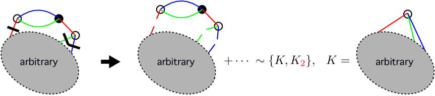
Fig. 1: Any level $n$ operator with loop is obtained by the join operation of the level $n-1$ operator $K$ with $K_{2}$.

Since the existence of the loops in a diagram means that the operator can be obtained by the join operation, the diagram that includes $({\color[rgb]{1,0,0}2})^{\prime}$, $({\color[rgb]{0,1,0}2})^{\prime}$ or $({\color[rgb]{0,0,1}2})^{\prime}$ does not correspond to the secondary operators by construction.

Moreover, each of the ingredients $({\color[rgb]{1,0,0}2})$, $({\color[rgb]{0,1,0}2})$ and $({\color[rgb]{0,0,1}2})$ can not be repeated if these have the same color because loops are always generated in such cases. For example, $({\color[rgb]{1,0,0}2})({\color[rgb]{1,0,0}2})$ generates one green-blue loop,

$$({\color[rgb]{1,0,0}2})({\color[rgb]{1,0,0}2})=\begin{picture}(60.0,10.0) \put(0.0,6.0){\color[rgb]{1,0,0}\line(1,0){30.0}} \put(0.0,-4.0){\color[rgb]{0,1,0}\line(1,0){10.0}} \put(10.0,-4.0){\color[rgb]{1,0,0}\line(1,0){10.0}} \put(20.0,-4.0){\color[rgb]{0,1,0}\line(1,0){10.0}} \put(0.0,0.0){{\color[rgb]{0,0,1}\qbezier(0.0,1.0)(10.0,0.0)(10.0,-4.0)}} \put(0.0,0.0){{\color[rgb]{0,0,1}\qbezier(30.0,1.0)(20.0,0.0)(20.0,-4.0)}} \put(10.0,-4.0){\circle{2.0}} \put(20.0,-4.0){\circle*{2.0}} \put(30.0,6.0){\color[rgb]{1,0,0}\line(1,0){30.0}} \put(30.0,-4.0){\color[rgb]{0,1,0}\line(1,0){10.0}} \put(40.0,-4.0){\color[rgb]{1,0,0}\line(1,0){10.0}} \put(50.0,-4.0){\color[rgb]{0,1,0}\line(1,0){10.0}} \put(30.0,0.0){{\color[rgb]{0,0,1}\qbezier(0.0,1.0)(10.0,0.0)(10.0,-4.0)}} \put(30.0,0.0){{\color[rgb]{0,0,1}\qbezier(30.0,1.0)(20.0,0.0)(20.0,-4.0)}} \put(40.0,-4.0){\circle{2.0}} \put(50.0,-4.0){\circle*{2.0}} \end{picture}~{}~{}.$$ (5.1)

This restriction on the repeated use of the ingredients with the same coloring is extended to the objects with subscript ${\color[rgb]{1,0,0}r}$, ${\color[rgb]{0,1,0}g}$, ${\color[rgb]{0,0,1}b}$, such as $(3W)_{\color[rgb]{1,0,0}r}$. For example, $(3W)_{\color[rgb]{1,0,0}r}({\color[rgb]{1,0,0}2})$ can always be split by cutting the lines depicted by the thick black lines as follows:

$$(3W)_{\color[rgb]{1,0,0}r}({\color[rgb]{1,0,0}2})=\begin{picture}(70.0,10.0) \put(0.0,6.0){\color[rgb]{1,0,0}\line(1,0){70.0}} \put(0.0,0.0){{\color[rgb]{0,0,1}\qbezier(0.0,1.0)(30.0,0.0)(30.0,-4.0)}} \put(0.0,0.0){{\color[rgb]{0,0,1}\qbezier(20.0,-4.0)(35.0,6.0)(50.0,-4.0)}} \put(0.0,0.0){{\color[rgb]{0,0,1}\qbezier(10.0,-4.0)(25.0,-14.0)(40.0,-4.0)}} \put(0.0,0.0){{\color[rgb]{0,0,1}\qbezier(60.0,-4.0)(60.0,0.0)(70.0,1.0)}} \put(0.0,-4.0){\color[rgb]{0,1,0}\line(1,0){10.0}} \put(10.0,-4.0){\color[rgb]{1,0,0}\line(1,0){10.0}} \put(20.0,-4.0){\color[rgb]{0,1,0}\line(1,0){10.0}} \put(30.0,-4.0){\color[rgb]{1,0,0}\line(1,0){10.0}} \put(40.0,-4.0){\color[rgb]{0,1,0}\line(1,0){10.0}} \put(50.0,-4.0){\color[rgb]{1,0,0}\line(1,0){10.0}} \put(60.0,-4.0){\color[rgb]{0,1,0}\line(1,0){10.0}} \put(10.0,-4.0){\circle{2.0}} \put(20.0,-4.0){\circle*{2.0}} \put(30.0,-4.0){\circle{2.0}} \put(40.0,-4.0){\circle*{2.0}} \put(50.0,-4.0){\circle{2.0}} \put(60.0,-4.0){\circle*{2.0}} \put(5.0,-7.0){\line(0,1){10.0}} \put(55.0,-7.0){\line(0,1){5.5}} \end{picture}~{}~{}.$$ (5.2)

In fact, (3.16), (3.22), (3.24), (3.31), (3.30), (3.32), (4.9)-(4.15) satisfy these restrictions. However, we have not been able to formulate rules for (4.16)-(4.18) by the computation up to level 6. In addition, we have seen to cases in which different “words” yield the same operator. Despite these incompleteness of the currently constructed rules, in principle, our procedure successfully generates all secondary operators level by level recursively.

References

- [1] F. David, “Planar Diagrams, Two-Dimensional Lattice Gravity and Surface Models,” Nucl. Phys. B 257, 45 (1985).
- [2] V. A. Kazakov, Alexander A. Migdal, and I. K. Kostov, “Critical Properties of Randomly Triangulated Planar Random Surfaces,” Phys. Lett. B 157, 295–300 (1985).
- [3] J. Ambjorn, B. Durhuus, and T. Jonsson, “Three-dimensional simplicial quantum gravity and generalized matrix models,” Mod. Phys. Lett. A6, 1133–1146 (1991).
- [4] N. Sasakura, “Tensor model for gravity and orientability of manifold,” Mod. Phys. Lett. A 6, 2613–2624 (1991).
- [5] P. H. Ginsparg, “Matrix models of 2-d gravity,”, In Trieste HEP Cosmol.1991:785-826, pages 785–826 (1991), arXiv:hep-th/9112013.
- [6] M. Gross, “Tensor models and simplicial quantum gravity in 2-d,” Nuc. Phys. B Proc. Suppl. 25, 144–149 (1992).
- [7] E. Witten, “An SYK-Like Model Without Disorder,” (2016), arXiv:1610.09758[hep-th].
- [8] R. Gurau, “The complete expansion of a SYK-like tensor model,” Nucl. Phys. B 916, 386–401 (2017), arXiv:1611.04032[hep-th].
- [9] R. Gurau, “Quenched equals annealed at leading order in the colored SYK model,” EPL 119(3), 30003 (2017), arXiv:1702.04228[hep-th].
- [10] S. Carrozza and A. Tanasa, “ Random Tensor Models,” Lett. Math. Phys. 106(11), 1531–1559 (2016), arXiv:1512.06718[hep-th].
- [11] I. R. Klebanov and G. Tarnopolsky, “Uncolored random tensors, melon diagrams, and the Sachdev-Ye-Kitaev models,” Phys. Rev. D 95(4), 046004 (2017), arXiv:1611.08915[hep-th].
- [12] D. J. Gross and V. Rosenhaus, “A Generalization of Sachdev-Ye-Kitaev,” JHEP 02, 093 (2017), arXiv:1610.01569[hep-th].
- [13] D. J. Gross and V. Rosenhaus, “The Bulk Dual of SYK: Cubic Couplings,” JHEP 05, 092 (2017), arXiv:1702.08016[hep-th].
- [14] D. J. Gross and V. Rosenhaus, “A line of CFTs: from generalized free fields to SYK,” JHEP 07, 086 (2017), arXiv:1706.07015[hep-th].
- [15] D. J. Gross and V. Rosenhaus, “All point correlation functions in SYK,” JHEP 12, 148 (2017), arXiv:1710.08113[hep-th].
- [16] C. Krishnan, S. Sanyal, and P. N. Bala Subramanian, “Quantum Chaos and Holographic Tensor Models,” JHEP 03, 056 (2017), arXiv:1612.06330[hep-th].
- [17] V. Bonzom and F. Combes, “Tensor models from the viewpoint of matrix models: the case of loop models on random surfaces,” Ann. Inst. H. Poincare Comb. Phys. Interact. 2(2), 1–47 (2015), arXiv:1304.4152[hep-th].
- [18] F. Ferrari, “The Large D Limit of Planar Diagrams,” (2017), arXiv:1701.01171[hep-th].
- [19] V. Bonzom, L. Lionni, and A. Tanasa, “Diagrammatics of a colored SYK model and of an SYK-like tensor model, leading and next-to-leading orders,” J. Math. Phys. 58(5), 052301 (2017), arXiv:1702.06944[hep-th].
- [20] R. Gurau, “The Schwinger Dyson equations and the algebra of constraints of random tensor models at all orders,” Nucl. Phys. B 865, 133–147 (2012), arXiv:1203.4965[hep-th].
- [21] V. Bonzom, “Revisiting random tensor models at large N via the Schwinger-Dyson equations,” JHEP 03, 160 (2013), arXiv:1208.6216[hep-th].
- [22] H. Itoyama, A. Mironov, and A. Morozov, “Rainbow tensor model with enhanced symmetry and extreme melonic dominance,” Phys. Lett. B 771, 180–188 (2017), arXiv:1703.04983[hep-th].
- [23] H. Itoyama, A. Mironov, and A. Morozov, “Ward identities and combinatorics of rainbow tensor models,” JHEP 06, 115 (2017), arXiv:1704.08648[hep-th].
- [24] H. Itoyama, A. Mironov, and A. Morozov, “Cut and join operator ring in tensor models,” Nucl. Phys. B 932, 52–118 (2018), arXiv:1710.10027[hep-th].
- [25] H. Itoyama, A. Mironov, and A. Morozov, “From Kronecker to tableau pseudo-characters in tensor models,” Phys. Lett. B 788, 76–81 (2019), arXiv:1808.07783[hep-th].
- [26] A. Mironov and A. Morozov, “Correlators in tensor models from character calculus,” Phys. Lett. B 774, 210–216 (2017), arXiv:1706.03667[hep-th].
- [27] F. David, “Loop Equations and Nonperturbative Effects in Two-dimensional Quantum Gravity,” Mod. Phys. Lett. A 5, 1019–1030 (1990).
- [28] A. Mironov and A. Morozov, “On the origin of Virasoro constraints in matrix models: Lagrangian approach,” Phys. Lett. B 252, 47–52 (1990).
- [29] J. Ambjorn and Yu. Makeenko, “Properties of Loop Equations for the Hermitean Matrix Model and for Two-dimensional Quantum Gravity,” Mod. Phys. Lett. A 5, 1753–1764 (1990).
- [30] H. Itoyama and Y. Matsuo, “Noncritical Virasoro algebra of matrix model and quantized string field,” Phys. Lett. B 255, 202–208 (1991).
- [31] H. Itoyama and Y. Matsuo, “ type constraints in matrix models at finite ,” Phys. Lett. B 262, 233–239 (1991).
- [32] R. Dijkgraaf, H. L. Verlinde, and E. P. Verlinde, “Loop equations and Virasoro constraints in nonperturbative 2-D quantum gravity,” Nucl. Phys. B 348, 435–456 (1991).
- [33] M. Fukuma, H. Kawai, and R. Nakayama, “Continuum Schwinger-dyson Equations and Universal Structures in Two-dimensional Quantum Gravity,” Int. J. Mod. Phys. A 6, 1385–1406 (1991).
- [34] M. Fukuma, H. Kawai, and R. Nakayama, “Infinite dimensional Grassmannian structure of two-dimensional quantum gravity,” Commun. Math. Phys. 143, 371–404 (1992).
- [35] A. Mironov and A. Morozov, “On the complete perturbative solution of one-matrix models,” Phys. Lett. B 771, 503–507 (2017), arXiv:1705.00976[hep-th].
- [36] A. Mironov and A. Morozov, “Sum rules for characters from character-preservation property of matrix models,” JHEP 08, 163 (2018), arXiv:1807.02409[hep-th].
- [37] A. Morozov, “Cut-and-join operators and Macdonald polynomials from the 3-Schur functions,” (2018), arXiv:1810.00395[hep-th].
- [38] A. Morozov, “On -representations of - and -deformed matrix models,” (2019), arXiv:1901.02811[hep-th].
- [39] V. Bonzom, R. Gurau, A. Riello, and V. Rivasseau, “Critical behavior of colored tensor models in the large limit,” Nucl. Phys. B 853, 174–195 (2011), arXiv:1105.3122[hep-th].
- [40] R. Gurau, “A generalization of the Virasoro algebra to arbitrary dimensions,” Nucl. Phys. B 852, 592–614 (2011), arXiv:1105.6072[hep-th].
- [41] J. Ben Geloun and S. Ramgoolam, “Counting Tensor Model Observables and Branched Covers of the 2-Sphere,” (2013), arXiv:1307.6490[hep-th].
- [42] P. Diaz and S.-J. Rey, “Orthogonal Bases of Invariants in Tensor Models,” JHEP 02, 089 (2018), arXiv:1706.02667[hep-th].
- [43] R. de Mello Koch, D. Gossman, and L. Tribelhorn, “Gauge Invariants, Correlators and Holography in Bosonic and Fermionic Tensor Models,” JHEP 09, 011 (2017), arXiv:1707.01455[hep-th].
- [44] J. Ben Geloun and S. Ramgoolam, “Tensor Models, Kronecker coefficients and Permutation Centralizer Algebras,” JHEP 11, 092 (2017), arXiv:1708.03524[hep-th].
- [45] A. Alexandrov, “Cut-and-join description of generalized Brezin-Gross-Witten model,” (2016), arXiv:1608.01627[hep-th].
- [46] A. Alexandrov, “Open intersection numbers, Kontsevich-Penner model and cut-and-join operators,” JHEP 08, 028 (2015), arXiv:1412.3772[hep-th].
- [47] A. Alexandrov, “Cut-and-Join operator representation for Kontsewich-Witten tau-function,” Mod. Phys. Lett. A 26, 2193–2199 (2011), arXiv:1009.4887[hep-th].
- [48] R. Wang, K. Wu, Z.-W. Yan, C.-H. Zhang, and W.-Z. Zhao, “ constraints for the hermitian one-matrix model,” (2019), arXiv:1901.10658[hep-th].