Experimental demonstration of fully contextual quantum correlations on an NMR quantum information processor

Abstract

The existence of contextuality in quantum mechanics is a fundamental departure from the classical description of the world. Currently, the quest to identify scenarios which cannot be more contextual than quantum theory is at the forefront of research in quantum contextuality. In this work, we experimentally test two inequalities, which are capable of revealing fully contextual quantum correlations, on a Hilbert space of dimension eight and four respectively, on an NMR quantum information processor. The projectors associated with the contextuality inequalities are first reformulated in terms of Pauli operators, which can be determined in an NMR experiment. We also analyze the behavior of each inequality under rotation of the underlying quantum state, which unitarily transforms it to another pure state.

I Introduction

Non-contextual hidden variable (NCHV) theories in which outcomes of measurements do not depend on other compatible measurements, have been shown not to reproduce quantum correlations Bell (1966); Kochen and Specker (1967). Quantum mechanics (QM) exhibits the property of contextuality Singh et al. (2017a); Raussendorf (2013); Howard et al. (2014) which implies that measurement results of observables depend upon other commuting observables which are within the same measurement test. Much recent research is going on in the direction of guessing the physical principle responsible for this form of contextuality Cabello (2011). The pertinent questions that arise include whether there is any theory more contextual than quantum mechanics and whether the simplest scenario in which more general theories cannot be more contextual than quantum mechanics can be identified Cabello (2013); Chiribella et al. (2011); Barnum et al. (2010); Pawlowski et al. (2009).

Contextuality tests correspond to the violation of certain inequalities involving expectation values, and the first such test was proposed by Kochen and Specker Kochen and Specker (1967) by using a single qutrit system (the KS theorem), and a modified KS scheme was constructed by Peres Peres (1991). State-independent Plastino and Cabello (2010); Badzia¸g et al. (2009); Cabello et al. (2015) tests use the set of observables such that for any quantum state there is no probability distribution which can describe the outcome of measurement of these observables on that state, hence these tests are able to reveal the contextual behavior of any state of the quantum system. On the other hand, the state-dependent Klyachko et al. (2008); Kurzyński and Kaszlikowski (2012); Sohbi et al. (2016) tests typically use fewer observables to show that no joint probability distribution can describe the measurement outcomes on a certain subset of states of the quantum system. The smallest indivisible physical system exhibiting quantum contextuality for repeatable measurements is a qutrit (a three-level quantum system) Bell (1966). The simplest state-dependent non-contextual inequality which is commonly referred to as the Klyachko-Can-Binicioglu-Shumovsky (KCBS) inequality Klyachko et al. (2008), for a qutrit requires five experiments, each of them involving two compatible yes-no tests Cabello (2013). Several experimental tests of quantum contextuality have been demonstrated by different groups using photons Zu et al. (2012); D’Ambrosio et al. (2013); Amselem et al. (2009); Nagali et al. (2012); Huang et al. (2013), ions Zhang et al. (2013); Leupold et al. (2018), neutrons Bartosik et al. (2009) and nuclear spins Moussa et al. (2010); Dogra et al. (2016).

In this paper, we experimentally demonstrate fully contextual quantum correlations via two different inequalities, on an NMR quantum information processor. The first inequality as proposed by Cabello Cabello (2013), utilizes ten projectors and requires five measurements on a state in a Hilbert space of dimension at least six. We demonstrate this inequality by realizing the six-dimensional subspace on states in an eight-dimensional Hilbert space. The second inequality as proposed by Nagali et. al Nagali et al. (2012), uses ten projectors and ten measurements which we implement on states in a four-dimensional Hilbert space. For experimental verification of both the inequalities, we decompose all the projectors involved in terms of Pauli operators. The advantage is two-fold: first, it reduces the need of performing quantum state tomography which is a resource-intensive procedure and second, the inequalities can be tested by using a fewer number of observables. The eight-dimensional and four-dimensional Hilbert spaces are physically realized using three and two NMR qubits, respectively. Violation of the inequalities as observed experimentally match well with theoretical predictions and have an experimental fidelity $\geq 0.96$. We also study the behavior of both the inequalities when the underlying quantum state undergoes a rotation. Our results imply that the violation of both inequalities follows a nonlinear trend with respect to the rotation angle of the underlying state. We also find that fully contextual quantum correlations on an eight-dimensional Hilbert space are more robust against state rotation, as compared to the ones on the four-dimensional Hilbert space, allowing a greater angle for violation.

The material in this paper is arranged as follows: Section II describes the fully contextual quantum correlations, the quantum state and the yes/no tests required to reveal correlations with zero non-contextual content and their experimental implementation on an eight-dimensional quantum system using three NMR qubits. Section III describes fully contextual quantum correlations in a four-dimensional Hilbert space, and its experimental implementation using two NMR qubits. Section IV contains a few concluding remarks.

II Fully contextual quantum correlations in an eight-dimensional Hilbert space

In this section, we first review a contextuality inequality which is capable of revealing fully contextual quantum correlations as developed by Cabello Cabello (2013), which requires a Hilbert space dimensionality of at least $6$. We then design a modified version of the inequality via decomposition of the projectors into Pauli matrices, for ease of experimental implementation. We experimentally test the inequality on an eight-level quantum system, physically realized via three NMR qubits.

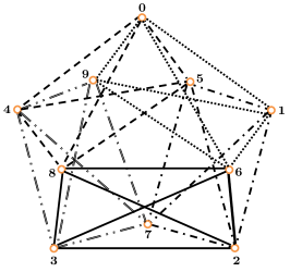
Figure 1: Orthogonality graph corresponding to the KCBS-twin inequality $\mathcal{K}$. Vertices correspond to projectors, while edges represent the orthogonality relationship between two vertices. Five sets of four interconnected vertices correspond to measurements involved in testing $\mathcal{K}$ and are differentiated by different edge line styles.

Table 1: Pauli operators for three qubits, used to decompose the corresponding projectors for the experimental demonstration of the inequality $\mathcal{K}$.

Pauli operators	Pauli operators
$A_{0}$ = $\mathds{1}\otimes\mathds{1}\otimes\sigma_{x}$	$A_{18}$ = $\sigma_{x}\otimes\sigma_{z}\otimes\sigma_{x}$
$A_{1}$ =$\mathds{1}\otimes\mathds{1}\otimes\sigma_{z}$	$A_{19}$ = $\sigma_{x}\otimes\sigma_{z}\otimes\sigma_{z}$
$A_{2}$ = $\mathds{1}\otimes\sigma_{x}\otimes\mathds{1}$	$A_{20}$ = $\sigma_{y}\otimes\mathds{1}\otimes\sigma_{y}$
$A_{3}$ = $\mathds{1}\otimes\sigma_{x}\otimes\sigma_{x}$	$A_{21}$ = $\sigma_{y}\otimes\sigma_{x}\otimes\sigma_{y}$
$A_{4}$ = $\mathds{1}\otimes\sigma_{x}\otimes\sigma_{z}$	$A_{22}$ = $\sigma_{y}\otimes\sigma_{y}\otimes\mathds{1}$
$A_{5}$ = $\mathds{1}\otimes\sigma_{y}\otimes\sigma_{y}$	$A_{23}$ = $\sigma_{y}\otimes\sigma_{y}\otimes\sigma_{x}$
$A_{6}$ = $\mathds{1}\otimes\sigma_{z}\otimes\mathds{1}$	$A_{24}$ = $\sigma_{y}\otimes\sigma_{y}\otimes\sigma_{z}$
$A_{7}$ = $\mathds{1}\otimes\sigma_{z}\otimes\sigma_{x}$	$A_{25}$ = $\sigma_{y}\otimes\sigma_{z}\otimes\sigma_{y}$
$A_{8}$ = $\mathds{1}\otimes\sigma_{z}\otimes\sigma_{z}$	$A_{26}$ = $\sigma_{z}\otimes\mathds{1}\otimes\mathds{1}$
$A_{9}$ = $\sigma_{x}\otimes\mathds{1}\otimes\mathds{1}$	$A_{27}$ = $\sigma_{z}\otimes\mathds{1}\otimes\sigma_{x}$
$A_{10}$ = $\sigma_{x}\otimes\mathds{1}\otimes\sigma_{x}$	$A_{28}$ = $\sigma_{z}\otimes\mathds{1}\otimes\sigma_{z}$
$A_{11}$ = $\sigma_{x}\otimes\mathds{1}\otimes\sigma_{z}$	$A_{29}$ = $\sigma_{z}\otimes\sigma_{x}\otimes\mathds{1}$
$A_{12}$ = $\sigma_{x}\otimes\sigma_{x}\otimes\mathds{1}$	$A_{30}$ = $\sigma_{z}\otimes\sigma_{x}\otimes\sigma_{x}$
$A_{13}$ = $\sigma_{x}\otimes\sigma_{x}\otimes\sigma_{x}$	$A_{31}$ = $\sigma_{z}\otimes\sigma_{x}\otimes\sigma_{z}$
$A_{14}$ = $\sigma_{x}\otimes\sigma_{x}\otimes\sigma_{z}$	$A_{32}$ = $\sigma_{z}\otimes\sigma_{y}\otimes\sigma_{y}$
$A_{15}$ = $\sigma_{x}\otimes\sigma_{y}\otimes\sigma_{x}$	$A_{33}$ = $\sigma_{z}\otimes\sigma_{z}\otimes\mathds{1}$
$A_{16}$ = $\sigma_{x}\otimes\sigma_{y}\otimes\sigma_{y}$	$A_{34}$ = $\sigma_{z}\otimes\sigma_{z}\otimes\sigma_{x}$
$A_{17}$ = $\sigma_{x}\otimes\sigma_{z}\otimes\mathds{1}$	$A_{35}$ = $\sigma_{z}\otimes\sigma_{z}\otimes\sigma_{z}$

The simplest test of quantum contextuality requires the measurement of five different projectors $\{\Pi_{i}\}$, $i\in\{0,1,2,3,4\}$ and $\Pi_{i}=|v_{i}\rangle\langle v_{i}|$, where $|v_{i}\rangle$ are unit vectors Klyachko et al. (2008). These projectors follow the exclusivity relation $P(\Pi_{i}=1)+P(\Pi_{i\oplus 1}=1)=1$, where $P(\Pi_{i}=1)$ represents the probability of obtaining the outcome $\Pi_{i}$, and addition is taken modulo five. For projective measurements, this relationship implies that only one of $\Pi_{i}$ or $\Pi_{i\oplus 1}$ can be obtained in a joint measurement of both. The corresponding test, termed as KCBS inequality Cabello (2013) is of the form

$$\frac{1}{2}\sum_{i=0}^{4}P(\Pi_{i}+\Pi_{i\oplus 1}=1)\overset{\text{NCHV}}{\leq}2\overset{\text{QM}}{\leq}\sqrt{5}\overset{\text{GP}}{\leq}\frac{5}{2},$$ (1)

where the inequalities correspond to the maximum value achievable for non-contextual hidden variable (NCHV) theories, quantum mechanics (QM) and generalized probabilistic (GP) theories.

Table 2: Product operators for a three-qubit system, mapped to the Pauli $z$ operators via the initial state transformation $\rho\rightarrow\rho_{i}=U_{i}.\rho.U^{\dagger}_{i}$.

Observable Expectation		Unitary Operator
$\langle\sigma_{3z}\rangle$ = Tr[$\rho_{1}.\sigma_{3z}$]		$U_{1}$=Identity
$\langle\sigma_{2z}\rangle$ = Tr[$\rho_{2}.\sigma_{2z}$]		$U_{2}$=Identity
$\langle\sigma_{2z}\sigma_{3z}\rangle$ = Tr[$\rho_{3}.\sigma_{3z}$]		$U_{3}=\rm{CNOT_{23}~{}}$
$\langle\sigma_{1z}\rangle$ = Tr[$\rho_{4}.\sigma_{1z}$]		$U_{4}$=Identity
$\langle\sigma_{1z}\sigma_{3z}\rangle$ = Tr[$\rho_{5}.\sigma_{3z}$]		$U_{5}=\rm{CNOT_{13}~{}}$
$\langle\sigma_{1z}\sigma_{2z}\rangle$ = Tr[$\rho_{6}.\sigma_{2z}$]		$U_{6}=\rm{CNOT_{12}~{}}$
$\langle\sigma_{1z}\sigma_{2z}\sigma_{3z}\rangle$ = Tr[$\rho_{7}.\sigma_{3z}$]		$U_{7}=\rm{CNOT_{23}~{}}.\rm{CNOT_{12}~{}}$

As is evident from Eqn. (1), the maximum violation that can be achieved in quantum mechanics is less than what can be attained if an underlying GP model is considered. Therefore, for the KCBS scenario, quantum correlations are not fully contextual. Recently, it has been shown that there exist tests of contextuality for which quantum correlations saturate the bound as imposed by GP models Amselem et al. (2012). For these scenarios, quantum correlations are either non-contextual or fully contextual. The simplest test of contextuality, capable of revealing fully contextual quantum correlations again requires only five measurements, but of ten different projectors $\{\Pi_{i}\}$ and is of the form,

$$\mathcal{K}=\frac{1}{2}\sum_{i=0}^{4}P(\Pi_{i}+\Pi_{i+1}+\Pi_{i+5}+\Pi_{i+7}=1)\overset{\text{NCHV}}{\leq}2\overset{\text{QM, GP}}{\leq}\frac{5}{2},$$ (2)

where the sum in the indices is defined such that $4+1=0$ and $3+7=5$. Since both the KCBS and the aforementioned inequality (Eqn. 2) require only five different measurements, the above scenario is termed as a twin inequality of KCBS, with the only difference that it is capable of revealing fully contextual quantum correlations and requires quantum systems having Hilbert space dimension at least six. We will henceforth refer to this inequality as the “KCBS-twin” inequality.

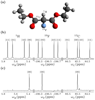
Figure 2: (a) Molecular structure of ¹³C-labeled diethyl fluoromalonate used to physically realize three qubits. NMR spectra of (b) the thermal equilibrium state and (c) the pseudopure state $|000\rangle$. Each peak is labeled with the logical state of the qubit which is passive during the transition. The horizontal scale represents the chemical shifts in ppm.

Table 3: NMR parameters for the three-qubit ¹³C-labeled diethyl fluoromalonate system.

Qubit	$\nu$ (Hz)	$J$ (Hz)	$~{}T_{1}$ (sec)	$T_{2}$ (sec)
$\rm{}^{1}H$	$3334.24$	$J_{HF}=47.5$	$3.4$	$1.6$
$\rm{}^{19}F$	$~{}-110999.94$	$J_{HC}=161.6$	$3.7$	$1.5$
$\rm{}^{13}C$	$12889.53$	$~{}J_{FC}=-191.5$	$3.6$	$1.3$

The scenario corresponding to the KCBS-twin inequality (Eqn. 2) can be represented by an exclusivity graph as shown in Fig. 1. In this graph, each vertex corresponds to a unit vector $|v_{i}\rangle$ used to construct the projectors $\Pi_{i}$, and two vertices are connected by an edge if and only if they are exclusive. From the graph it is possible to identify five different measurements $\mathcal{M}_{i}$ which are defined as

$$\mathcal{M}_{i}=\{\Pi_{i},\Pi_{i+1},\Pi_{i+5},\Pi_{i+7}\},\quad\forall i\in\{0,1,...,9\}.$$ (3)

These measurements can be identified from the graph in Fig. 1 by five sets of four interconnected vertices, each represented by a different line style.

An explicit form of the KCBS-twin inequality (Eqn. 2) which saturates the QM and GP bound can be obtained if we consider the unit vectors $|v_{i}\rangle$ defined as:

$$\langle v_{0}|\equiv \frac{1}{\sqrt{8}}(\sqrt{2},-\sqrt{2},0,0,2,0,0,0),$$ (4a)

$$\langle v_{1}|\equiv \frac{1}{\sqrt{8}}(\sqrt{2},0,0,\sqrt{2},-1,\sqrt{3},0,0),$$ (4b)

$$\langle v_{2}|\equiv \frac{1}{2}(1,-1,-1,-1,0,0,0,0),$$ (4c)

$$\langle v_{3}|\equiv \frac{1}{2}(1,-1,1,1,0,0,0,0),$$ (4d)

$$\langle v_{4}|\equiv \frac{1}{\sqrt{8}}(\sqrt{2},0,0,-\sqrt{2},-1,\sqrt{3},0,0),$$ (4e)

$$\langle v_{5}|\equiv \frac{1}{\sqrt{8}}(\sqrt{2},0,-\sqrt{2},0,-1,-\sqrt{3},0,0),$$ (4f)

$$\langle v_{6}|\equiv \frac{1}{\sqrt{8}}(\sqrt{2},0,\sqrt{2},0,-1,-\sqrt{3},0,0),$$ (4g)

$$\langle v_{7}|\equiv \frac{1}{2}(1,1,1,-1,0,0,0,0),$$ (4h)

$$\langle v_{8}|\equiv \frac{1}{\sqrt{8}}(\sqrt{2},\sqrt{2},0,0,2,0,0,0),$$ (4i)

$$\langle v_{9}|\equiv \frac{1}{2}(1,1,-1,1,0,0,0,0).$$ (4j)

The state $|\psi\rangle$ on which the measurements $\mathcal{M}_{i}$ will be performed is chosen as

$$\langle\psi|\equiv(1,0,0,0,0,0,0,0),$$ (5)

so that $\langle v_{i}|\psi\rangle=\frac{1}{2}$ $\forall\,i\in\{0,1,...,9\}$ which subsequently ensures the exclusivity relation $P(\Pi_{i}+\Pi_{i+1}+\Pi_{i+5}+\Pi_{i+7}=1)=1$, $i=0,1,...,4$.

In order to evaluate the KCBS-twin inequality experimentally, we first decompose the projectors involved in terms of Pauli operators, $\sigma_{j}$, $j\in\{x,y,z\}$ for three qubits given by:

$$\Pi_{0} =\frac{1}{16}\left(\begin{aligned} &-A_{0}+A_{1}+2A_{6}-A_{7}+A_{8}+\sqrt{2}(A_{9}-A_{10}+A_{11}+A_{17}-A_{18}+A_{19}-A_{20}-A_{25})\\ &\quad-A_{27}-A_{28}-A_{34}-A_{35}+2\mathds{1}\end{aligned}\right),$$ (6a)

$$\Pi_{1} =\frac{1}{32}\left(\begin{aligned} &-\sqrt{3}A_{0}-A_{1}+2A_{3}-2A_{5}+2A_{6}-\sqrt{3}A_{7}+A_{8}\\ &\quad+\sqrt{2}\left(-A_{9}+\sqrt{6}A_{10}-A_{11}+\sqrt{6}A_{12}-A_{13}-\sqrt{6}A_{14}+A_{15}+A_{16}-A_{17}+\sqrt{6}A_{18}\right)\\ &\quad+\sqrt{2}\left(-A_{19}-\sqrt{6}A_{20}-A_{21}+\sqrt{6}A_{22}-A_{23}-\sqrt{6}A_{24}-\sqrt{6}A_{25}\right)\\ &\quad+\sqrt{3}A_{27}+A_{28}+2A_{30}-2A_{32}-2A_{33}+\sqrt{3}A_{34}+3A_{35}+4\mathds{1}\end{aligned}\right),$$ (6b)

$$\Pi_{2} =\frac{1}{8}\left(\begin{aligned} -A_{4}+A_{5}-A_{7}+A_{26}-A_{31}+A_{32}-A_{34}+\mathds{1}\end{aligned}\right),$$ (6c)

$$\Pi_{3} =\frac{1}{8}\left(A_{4}-A_{5}-A_{7}+A_{26}+A_{31}-A_{32}-A_{34}+\mathds{1}\right),$$ (6d)

$$\Pi_{4} =\frac{1}{32}\left(\begin{aligned} &-\sqrt{3}A_{0}-A_{1}-2A_{3}+2A_{5}+2A_{6}-\sqrt{3}A_{7}+A_{8}\\ &\quad+\sqrt{2}\left(-A_{9}+\sqrt{6}A_{10}-A_{11}-\sqrt{6}A_{12}+A_{13}+\sqrt{6}A_{14}-A_{15}-A_{16}-A_{17}+\sqrt{6}A_{18}\right)\\ &\quad+\sqrt{2}\left(-A_{19}-\sqrt{6}A_{20}+A_{21}-\sqrt{6}A_{22}+A_{23}+\sqrt{6}A_{24}-\sqrt{6}A_{25}\right)\\ &\quad+\sqrt{3}A_{27}+A_{28}-2A_{30}+2A_{32}-2A_{33}+\sqrt{3}A_{34}+3A_{35}+4\mathds{1}\end{aligned}\right),$$ (6e)

$$\Pi_{5} =\frac{1}{32}\left(\begin{aligned} &\sqrt{3}A_{0}+A_{1}-2A_{2}-2A_{4}+2A_{6}+\sqrt{3}A_{7}-A_{8}\\ &\quad+\sqrt{2}\left(-A_{9}-\sqrt{6}A_{10}-A_{11}+A_{12}+\sqrt{6}A_{13}+A_{14}+\sqrt{6}A_{16}-A_{17}-\sqrt{6}A_{18}\right)\\ &\quad+\sqrt{2}\left(\-A_{19}+\sqrt{6}A_{20}-\sqrt{6}A_{21}+A_{22}+\sqrt{6}A_{23}+A_{24}+\sqrt{6}A_{25}\right)\\ &\quad-\sqrt{3}A_{27}+3A_{28}-2A_{29}-2A_{31}-2A_{33}-\sqrt{3}A_{34}+A_{35}+4\mathds{1}\end{aligned}\right),$$ (6f)

$$\Pi_{6} =\frac{1}{32}\left(\begin{aligned} &\sqrt{3}A_{0}+A_{1}+2A_{2}+2A_{4}+2A_{6}+\sqrt{3}A_{7}-A_{8}\\ &\quad+\sqrt{2}\left(-A_{9}-\sqrt{6}A_{10}-A_{11}-A_{12}-\sqrt{6}A_{13}-A_{14}-\sqrt{6}A_{16}-A_{17}-\sqrt{6}A_{18}\right)\\ &\quad+\sqrt{2}\left(-A_{19}+\sqrt{6}A_{20}+\sqrt{6}A_{21}-A_{22}-\sqrt{6}A_{23}-A_{24}+\sqrt{6}A_{25}\right)\\ &\quad-\sqrt{3}A_{27}+3A_{28}+2A_{29}+2A_{31}-2A_{33}-\sqrt{3}A_{34}+A_{35}+4\mathds{1}\end{aligned}\right),$$ (6g)

$$\Pi_{7} =\frac{1}{8}\left(A_{4}+A_{5}+A_{7}+A_{26}+A_{31}+A_{32}+A_{34}+\mathds{1}\right),$$ (6h)

$$\Pi_{8} =\frac{1}{16}\left(\begin{aligned} &+A_{0}+A_{1}+2A_{6}+A_{7}+A_{8}\\ &\quad+\sqrt{2}\left(A_{9}+A_{10}+A_{11}+A_{17}+A_{18}+A_{19}+A_{20}+A_{25}\right)\\ &\quad+A_{27}-A_{28}+A_{34}-A_{35}+2\mathds{1}\end{aligned}\right),$$ (6i)

$$\Pi_{9} =\frac{1}{8}\left(-A_{4}-A_{5}+A_{7}+A_{26}-A_{31}-A_{32}+A_{34}+\mathds{1}\right).$$ (6j)

where $A_{i}$ s are given in Table 1. In NMR, the observed $z$ magnetization of a nuclear spin in a quantum state is proportional to the expectation value of the $\sigma_{z}$ operator of the spin in that state. The time-domain NMR signal, i.e., the free-induction decay with appropriate phase gives Lorentzian peaks when Fourier transformed. These normalized experimental intensities give an estimate of the expectation value of $\sigma_{z}$ of the quantum state. The observables of interest are $A_{1},A_{6},A_{8},A_{26},A_{28},A_{33},A_{35}$ for the eight-dimensional Hilbert space being considered. The task of experimentally demonstrating the inequality $\mathcal{K}$ (given in Eqn. 2) on an NMR quantum information processor becomes particularly accessible while dealing with the Pauli basis, since the NMR signal is proportional to ensemble average of the $\sigma_{z}$ operator. Thus measurement of the expectation value of the projectors $\{\Pi_{i}\}$ involved becomes simplified when they are decomposed into Pauli operators Singh et al. (2018); Gaikwad et al. (2018); Dogra et al. (2016) given by the observables $\{A_{i}\}$.

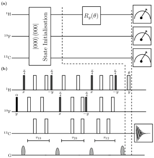
Figure 3: (a) Quantum circuit for state preparation; the parameter $\theta$ in the unitary $R_{y}(\theta)$ is used to generate different quantum states. (b) Corresponding NMR pulse sequence for the quantum circuit. The sequence of pulses before the first dashed black line achieves initialization of the state into the pseudopure $|000\rangle$ state. The value of the flip angle $\alpha$ is kept fixed at $57.87^{\circ}$, while the flip angle $\theta$ is varied over a range of values. The broad unfilled rectangles denote $\pi$ pulses, and the flip angle and phases of the other pulses written below each pulse. The time intervals $\tau_{12}$, $\tau_{13}$, $\tau_{23}$ are set to $\frac{1}{2J_{HF}}$, $\frac{1}{2J_{HC}}$, $\frac{1}{2J_{FC}}$, respectively.

Using the decomposition given in Eqn. (6), the inequality $\mathcal{K}$ (given in Eqn. 2) can be re-written as:

$$\mathcal{K}=\frac{1}{8}\text{Tr}\left[A\cdot\rho\right]\overset{\text{NCHV}}{\leq}2\overset{\text{QM, GP}}{\leq}\frac{5}{2},$$ (7)

where $\rho=|\psi\rangle\langle\psi|$ and

$$A=A_{1}+4A_{6}+A_{8}+4A_{26}+A_{28}-2A_{33}+A_{35}+10\mathds{1}.$$ (8)

By experimentally measuring the expectation value of each observable $A_{i}$ for the state $\rho$, the value of the inequality $\mathcal{K}$ can be estimated. The explicit mapping of expectation value of the observables onto Pauli $z$ operators for three qubits is given in Table 2. The underlying state $|\psi\rangle$ is unitarily rotated by an angle $\theta$ as:

$$|\psi(\theta)\rangle=U_{\theta}\otimes\mathds{1}\otimes\mathds{1}|\psi\rangle,$$ (9)

where,

$$U_{\theta}=\begin{bmatrix}\cos\frac{\theta}{2}&-\sin\frac{\theta}{2}\\ \sin\frac{\theta}{2}&\cos\frac{\theta}{2}\end{bmatrix}$$ (10)

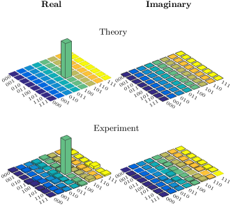
Figure 4: Real (left) and imaginary (right) parts of the theoretically expected and the experimentally reconstructed tomographs of the $\langle\psi_{1}|=(0,0,0,0,1,0,0,0)$ state in the eight-dimensional quantum system, with an experimental state fidelity of 0.97.

To experimentally implement the KCBS-twin inequality capable of revealing fully contextual quantum correlations for an eight-dimensional quantum system, we used the molecule of ¹³C -labeled diethyl fluoromalonate dissolved in acetone-D6, with the ¹H, ¹⁹F and ¹³C spin-1/2 nuclei being encoded as ‘qubit one’, ‘qubit two’ and ‘qubit three’, respectively (see Fig 2 for the molecular structure and corresponding NMR spectrum of the PPS state, and Table 3 for details of the experimental NMR parameters). The NMR Hamiltonian for a three-qubit system is given by Singh et al. (2018)

$$\mathcal{H}=-\sum_{i=1}^{3}v_{i}I^{i}_{z}+\sum_{i>j,i=1}^{3}J_{ij}I^{i}_{z}I^{j}_{z}$$ (11)

where the indices $i,j$ = 1, 2, or 3 label the qubit, $\nu_{i}$ is the chemical shift of the $i$th qubit in the rotating frame, $J_{{ij}}$ is the scalar coupling interaction strength, and $I_{z}^{{i}}$ is $z$-component of the spin angular momentum operator of the $i^{th}$ qubit. The system was initialized in a pseudopure state (PPS), i.e., $|000\rangle$, using the spatial averaging technique Mitra et al. (2007) with the density operator given by

$$\rho_{000}=\frac{1-\epsilon}{2^{3}}\mathds{I}_{8}+\epsilon|000\rangle\langle 000|$$ (12)

where $\epsilon$ is proportional to the spin polarization and $\mathds{I}_{8}$ is the $8\times 8$ identity operator. The fidelity of the experimentally prepared PPS state was computed to be 0.96 using the fidelity measure Zhang et al. (2014). Full quantum state tomography (QST) Leskowitz and Mueller (2004); Singh et al. (2016) was performed to experimentally reconstruct the density operator via a set of preparatory pulses $\{III,IIY,IYY,YII,XYX,XXY,XXX\}$, where $I$ implies no operation, and $X(Y)$ denotes a qubit-selective rf pulse of flip angle $90^{\circ}$ of phase $x(y)$.

Experiments were performed at room temperature (294 K) on a Bruker Avance III 600-MHz FT-NMR spectrometer equipped with a QXI probe. Local unitary operations were achieved by using highly accurate and calibrated spin selective transverse rf pulses of suitable amplitude, phase, and duration. Nonlocal unitary operations were achieved by free evolution under the system Hamiltonian, of suitable duration under the desired scalar coupling with the help of embedded $\pi$ refocusing pulses. The durations of the $\frac{\pi}{2}$ pulses for ¹H, ¹⁹F, and ¹³C nuclei were 9.36 $\mu$s at 18.14 W power level, 23.25 $\mu$s at a power level of 42.27 W, and 15.81 $\mu$s at a power level of 179.47 W, respectively.

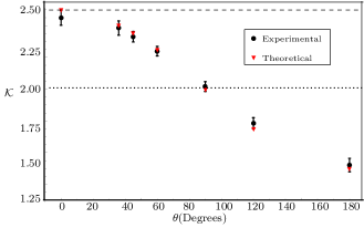
Figure 5: Graph representing quantum correlations corresponding to the inequality $\mathcal{K}$ for various states rotated by angle $\theta$ from the initial state $|\psi\rangle$.

Table 4: Theoretically computed and experimentally measured values of quantum correlations corresponding to the inequality $\mathcal{K}$ for various states, rotated by angle $\theta$, from the initial state $|\psi\rangle$.

$\theta$	Theoretical	Experimental
180∘	1.500	1.522$\pm$0.042
120∘	1.750	1.785$\pm$0.035
90∘	2.000	2.016$\pm$0.031
60∘	2.250	2.239$\pm$0.030
45∘	2.353	2.330$\pm$0.033
36∘	2.404	2.385$\pm$0.045
0∘	2.500	2.449$\pm$0.046

The quantum circuit to construct the states required to test fully contextual quantum correlations is shown in Fig. 3(a) and the corresponding NMR pulse sequence is shown in Fig 3(b). Different states can be prepared by varying the value of the flip angle $\theta$ of the rf pulse. We prepared seven different states by varying the flip angle $\theta$ to attain a range of values: $180^{\circ},120^{\circ},90^{\circ},60^{\circ},45^{\circ},36^{\circ},0^{\circ}$. The state prepared with $\theta=180^{\circ}$ gives the minimum value of $\mathcal{K}$, while the state prepared without applying any rf pulse ($\theta=0^{\circ}$) gives the maximum value. All the states required to demonstrate the KCBS-twin inequality on an 8-dimensional Hilbert space which are capable of revealing the transformation from classical correlations to fully contextual correlations, were experimentally prepared with state fidelities of $\geq 0.96$. The tomograph of one such experimentally reconstructed state with flip angle $\theta=180^{\circ}$ with state fidelity 0.97 is depicted in Fig. 4. For each of the initial states, the contextuality test was repeated three times. The mean values and the corresponding error bars were computed and the result is shown in Fig 5, where the inequality values are plotted for different values of the parameter $\theta$. The maximum of the sum of probabilities using classical theory is $2$ and the maximum of sum of probabilities using quantum theory is $2.5$, which are depicted by dotted and dashed lines respectively in Fig 5. The theoretically computed and experimentally obtained values of the inequality for different values of the $\theta$ parameter are tabulated in Table 4. The theoretical and experimental values match well, within the limits of experimental errors. From Fig. 5 it is also seen that the violation observed for the KCBS-twin inequality decreases as the original state $|\psi\rangle$ is rotated through an angle $\theta$, with no violation when the transformed state is orthogonal to the original state. Furthermore, the plot is nonlinear, indicating that smaller rotations lead to minor changes in violation, while larger rotations may also lead to observing no violation at all.

III Fully contextual quantum correlations in a four-dimensional Hilbert space

Figure 6: Orthogonality graph corresponding to the inequality $\mathcal{C}$. Vertices correspond to projectors and two vertices are connected by an edge if they are orthogonal.

In this section, we first review a contextuality inequality which is capable of revealing fully contextual quantum correlations as developed by Nagali et. al Nagali et al. (2012) which utilizes states in a Hilbert space of dimension at least four. We provide a modified version of the inequality by decomposition into Pauli matrices which we experimentally test on a four-level quantum system using two NMR qubits. Fully contextual quantum correlations can also be achieved for scenarios other than KCBS. As shown in Reference Nagali et al. (2012), one such scenario entails measurements corresponding to ten different projectors $\Pi_{j}=|u_{j}\rangle\langle u_{j}|$, $j=\{0,1,...,9\}$. In this particular scenario, the projectors follow exclusivity relationships as depicted in Fig. 6, where each vertex represents a projector $\Pi_{i}$ and two projectors are connected by an edge if and only if they are exclusive. The corresponding test of contextuality is then given by the inequality:

$$\mathcal{C}=\sum_{i=0}^{9}P(\Pi_{i}=1)\overset{\text{NCHV}}{\leq}3\overset{\text{QM, GP}}{\leq}\frac{7}{2}.$$ (13)

Table 5: Product operators for a two-qubit system mapped onto the Pauli $z$ operators via the initial state $\rho\rightarrow\rho_{i}=U_{i}.\rho.U^{\dagger}_{i}$.

Observable Expectation		Unitary Operator
$\langle\sigma_{1x}\sigma_{2x}\rangle$ = Tr[$\rho_{1}.\sigma_{2z}$]		$U_{1}={\rm{CNOT_{12}~{}}}Y_{2}Y_{1}$
$\langle\sigma_{1y}\sigma_{2y}\rangle$ = Tr[$\rho_{2}.\sigma_{2z}$]		$U_{2}={\rm{CNOT_{12}~{}}}\overline{X}_{2}\overline{X}_{1}$
$\langle\sigma_{1z}\rangle$ = Tr[$\rho_{3}.\sigma_{1z}$].		$U_{3}$=Identity
$\langle\sigma_{1z}\sigma_{2z}\rangle$ = Tr[$\rho_{4}.\sigma_{2z}$]		$U_{4}=\rm{CNOT_{12}~{}}$
$\langle\sigma_{2z}\rangle$ = Tr[$\rho_{5}.\sigma_{2z}$]		$U_{5}$=Identity

The scenario is reminiscent of the KCBS-twin inequality discussed in the previous section, however this test requires ten different measurements rather than five and is capable of revealing fully contextual quantum correlations in a much smaller Hilbert space (of minimum dimension four). The inequality can be explicitly tested if we consider the unit vectors $|u_{i}\rangle$ as follows:

$$\langle u_{0}|\equiv \frac{1}{\sqrt{2}}(0,0,1,1),$$ (14a)

$$\langle u_{1}|\equiv \frac{1}{2}(1,-1,1,-1),$$ (14b)

$$\langle u_{2}|\equiv \frac{1}{2}(1,-1,-1,1),$$ (14c)

$$\langle u_{3}|\equiv \frac{1}{\sqrt{2}}(1,0,0,-1),$$ (14d)

$$\langle u_{4}|\equiv \frac{1}{2}(1,1,1,1),$$ (14e)

$$\langle u_{5}|\equiv \frac{1}{\sqrt{2}}(0,1,0,-1),$$ (14f)

$$\langle u_{6}|\equiv \frac{1}{2}(-1,1,1,1),$$ (14g)

$$\langle u_{7}|\equiv \frac{1}{\sqrt{2}}(1,0,0,1),$$ (14h)

$$\langle u_{8}|\equiv \frac{1}{2}(1,1,1,-1),$$ (14i)

$$\langle u_{9}|\equiv \frac{1}{2}(1,1,-1,1).$$ (14j)

The corresponding projective measurements are of the form

$$\mathcal{M}_{j}=\{\Pi_{j},\mathds{1}-\Pi_{j}\}\quad\forall\,j\in\{0,1,...,9\},$$ (15)

which are performed on the state

$$\langle\phi|\equiv(0,0,0,1).$$ (16)

For the experimental implementation of the inequality, we again decompose the projectors $\{\Pi_{j}\}$ in terms of Pauli operators :

$$\Pi_{0}= \frac{1}{4}(-\sigma_{z}\otimes\mathds{1}-\sigma_{z}\otimes\sigma_{x}+\mathds{1}\otimes\sigma_{x}+\mathds{1}\otimes\mathds{1}),$$ (17a)

$$\Pi_{1}= \frac{1}{4}(\sigma_{x}\otimes\mathds{1}-\sigma_{x}\otimes\sigma_{x}-\mathds{1}\otimes\sigma_{x}+\mathds{1}\otimes\mathds{1}),$$ (17b)

$$\Pi_{2}= \frac{1}{4}(-\sigma_{x}\otimes\mathds{1}+\sigma_{x}\otimes\sigma_{x}-\mathds{1}\otimes\sigma_{x}+\mathds{1}\otimes\mathds{1}),$$ (17c)

$$\Pi_{3}= \frac{1}{4}(-\sigma_{x}\otimes\sigma_{x}+\sigma_{y}\otimes\sigma_{y}+\sigma_{z}\otimes\sigma_{z}+\mathds{1}\otimes\mathds{1}),$$ (17d)

$$\Pi_{4}= \frac{1}{4}(\sigma_{x}\otimes\mathds{1}+\sigma_{x}\otimes\sigma_{x}+\mathds{1}\otimes\sigma_{x}+\mathds{1}\otimes\mathds{1}),$$ (17e)

$$\Pi_{5}= \frac{1}{4}(-\sigma_{x}\otimes\mathds{1}+\sigma_{x}\otimes\sigma_{z}-\mathds{1}\otimes\sigma_{z}+\mathds{1}\otimes\mathds{1}),$$ (17f)

$$\Pi_{6}= \frac{1}{4}(-\sigma_{x}\otimes\sigma_{z}+\sigma_{y}\otimes\sigma_{y}-\sigma_{z}\otimes\sigma_{x}+\mathds{1}\otimes\mathds{1}),$$ (17g)

$$\Pi_{7}= \frac{1}{4}(\sigma_{x}\otimes\sigma_{x}-\sigma_{y}\otimes\sigma_{y}+\sigma_{z}\otimes\sigma_{z}+\mathds{1}\otimes\mathds{1}),$$ (17h)

$$\Pi_{8}= \frac{1}{4}(\sigma_{x}\otimes\sigma_{z}+\sigma_{y}\otimes\sigma_{y}+\sigma_{z}\otimes\sigma_{x}+\mathds{1}\otimes\mathds{1}),$$ (17i)

$$\Pi_{9}= \frac{1}{4}(-\sigma_{x}\otimes\sigma_{z}-\sigma_{y}\otimes\sigma_{y}+\sigma_{z}\otimes\sigma_{x}+\mathds{1}\otimes\mathds{1}).$$ (17j)

Using Eqn. (13) and Eqn. (17), the inequality $\mathcal{C}$ can be re-written as

$$\mathcal{C}=\frac{1}{4}\text{Tr}\left[B\cdot\rho^{\prime}\right]\overset{\text{NCHV}}{\leq}3\overset{\text{QM, GP}}{\leq}\frac{7}{2},$$ (18)

where $\rho^{\prime}=|\phi\rangle\langle\phi|$ and

$$B=B_{0}+B_{1}-B_{2}+2B_{3}-B_{4}+10\mathds{1},$$ (19)

with

$$B_{0} =\sigma_{x}\otimes\sigma_{x},$$ (20)

$$B_{1} =\sigma_{y}\otimes\sigma_{y},$$

$$B_{2} =\sigma_{z}\otimes\mathds{1},$$

$$B_{3} =\sigma_{z}\otimes\sigma_{z},$$

$$B_{4} =\mathds{1}\otimes\sigma_{z}.$$

The underlying state $|\phi\rangle$ is unitarily rotated by an angle $\theta$ as:

$$|\phi(\theta)\rangle=U_{\theta}\otimes\mathds{1}|\phi\rangle,$$ (21)

where $U_{\theta}$ has been defined in Eqn. (10).

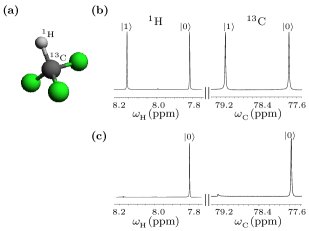
Figure 7: (a) Molecular structure of ¹³C-labeled chloroform used as a two-qubit quantum system. NMR spectra of (b) the thermal equilibrium state and (c) the pseudopure state $|00\rangle$. Each peak is labeled with the logical state of the qubit which is passive during the transition. Horizontal scale represents the chemical shifts in ppm.

By experimentally evaluating the expectation value of the observables $B_{j}$, the value of the inequality $\mathcal{C}$ can be estimated. To implement the non-contextual inequality capable of revealing fully contextual quantum correlations on a four-dimensional quantum system, the molecule of ¹³C-enriched chloroform dissolved in acetone-D6 was used, with the ¹H and ¹³C spins being labeled as ‘qubit one’ and ‘qubit two’, respectively (see Fig. 7 and Table 6 for details of the experimental parameters).

Table 6: NMR parameters for ¹³C-labeled chloroform used as a two-qubit quantum system.

Qubit	$\nu$ (Hz)	$~{}J$ (Hz)	$T_{1}$ (sec)	$T_{2}$ (sec)
$\rm{}^{1}H$	$4787.86$	$~{}J_{HC}=215.11$	$~{}7.9$	$2.95$
$\rm{}^{13}C$	$11814.09$		$~{}16.6$	$0.3$

The Hamiltonian for a two-qubit system is given by Gaikwad et al. (2018)

$${\mathcal{H}}=-\nu_{{\rm H}}I_{z}^{{\rm H}}-\nu_{{\rm C}}I_{z}^{{\rm C}}+J_{{\rm HC}}I_{z}^{{\rm H}}I_{z}^{{\rm C}}$$ (22)

where $\nu_{{\rm H}}$, $\nu_{{\rm C}}$ are the chemical shifts, $I_{z}^{{\rm H}}$, $I_{z}^{{\rm C}}$ are the $z$-components of the spin angular momentum operators of the ¹H and ¹³C spins respectively, and J_HC is the scalar coupling constant. The system was initialized in the pseudopure state (PPS) $|00\rangle$, using the spatial averaging technique Oliveira et al. (2007); Singh et al. (2017b) with the density operator given by

$$\rho_{00}=\frac{1}{4}(1-\epsilon)\mathds{I}_{4}+\epsilon|00\rangle\langle 00|$$ (23)

where $\mathds{I}_{4}$ is the $4\times 4$ identity operator, $\epsilon$ is proportional to the spin polarization and can be evaluated from the ratio of magnetic and thermal energies of an ensemble of magnetic moments $\mu$ in a magnetic field $B$ at temperature $T$; $\epsilon\thicksim\frac{\mu B}{k_{B}T}$ and at room temperature and for a $B\approx$ 10 Tesla, $\epsilon\approx\rm{10^{-5}}$. The state fidelity of the experimentally prepared PPS was computed to be 0.99. For the experimental reconstruction of density operator full quantum state tomography (QST) was performed using a set of preparatory pulses $\{II,IX,IY,XX\}$. Most of the experimental details are the same as for the three-qubit case. The durations of $\frac{\pi}{2}$ pulses for ¹H, ¹³C nuclei were 9.56 $\mu$s at power level 18.14 W and 16.15 $\mu$s at a power level of 179.47 W, respectively.

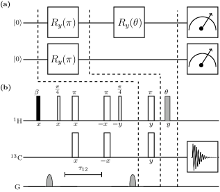
Figure 8: (a) Quantum circuit for the required state, generated randomly generated with the different flip angles. (b) NMR pulse sequence for the corresponding quantum circuit. The sequence of pulses before the first dashed black line achieves state initialization into the $|00\rangle$ state. The value of the flip angle $\beta$ is kept fixed at $59.69^{\circ}$, while the pulse rf flip angle $\theta$ is varied. The time interval $\tau_{12}$ is set to $\frac{1}{2J_{HC}}$.

Let $\pi_{i}$ be the observables (projectors) whose expectation value is to be measured in a state $\rho=|\psi\rangle\langle\psi|$. Instead of measuring $\langle\pi\rangle$, the state $\rho$ can be mapped to $\rho_{i}$ by using $\rho_{i}=U_{i}.\rho.U_{i}^{\dagger}$ followed by a $z$-magnetization measurement of one of the qubits Gaikwad et al. (2018). Table 5 details the mapping of Pauli basis operators (used in this paper) to the single-qubit Pauli $z$ operator, where $X,\overline{X},Y$ and $\overline{Y}$ represent the $\frac{\pi}{2}$ rotations with phases $x,-x,y$ and $-y$, respectively. The observables of interest are $B_{0},B_{1},B_{2},B_{3},B_{4}$ for the four-dimensional Hilbert space under consideration.

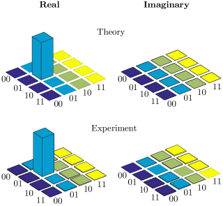
Figure 9: Real (left) and imaginary (right) parts of the theoretical and experimental tomographs of the $\langle\phi_{1}|=(0,-1,0,0)$ state in the four-dimensional Hilbert space, prepared with an experimental state fidelity of 0.99.

The quantum circuit to achieve the required states to test the inequality $\mathcal{C}$ on a four-dimensional quantum system is shown in Fig. 8(a) and the corresponding NMR pulse sequence is shown in Fig. 8(b). Eight different states were generated by varying the flip angle $\theta$ over a range of values: $180^{\circ},120^{\circ},90^{\circ},69.23^{\circ},60^{\circ},45^{\circ},30^{\circ},0^{\circ}$. The state that is prepared with the flip angle $\theta=180^{\circ}$ gives the minimum value of $\mathcal{C}$, while the state which is prepared without applying any rf pulse ($\theta=0^{\circ}$) gives the maximum value. All the states required for testing the inequality on the four-dimensional quantum system were experimentally prepared with state fidelities $\geq 0.97$. The tomograph for one such experimentally prepared state with the flip angle $\theta=180^{\circ}$ and state fidelity 0.99 is depicted in Fig. 9.

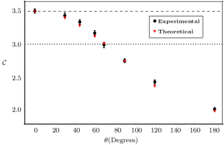
Figure 10: Quantum correlations corresponding to the inequality $\mathcal{C}$ for various states plotted for different initial states $|\phi\rangle$, as a function of the $\theta$ parameter.

Table 7: Theoretically computed and experimentally measured values of quantum correlations corresponding to the inequality $\mathcal{C}$ for different quantum states parameterized by the angle $\theta$.

$\theta$	Theoretical	Experimental
180∘	2.000	2.024$\pm$0.025
120∘	2.375	2.433$\pm$0.031
90∘	2.750	2.754$\pm$0.029
69.23∘	3.016	2.989$\pm$0.040
60∘	3.125	3.171$\pm$0.034
45∘	3.280	3.334$\pm$0.035
30∘	3.399	3.434$\pm$0.040
0∘	3.500	3.501$\pm$0.032

For each of these eight different initial states, the contextuality test was repeated three times. The mean values and the corresponding error bars were calculated and result is shown in Fig. 10, where the inequality values are plotted for different $\theta$ values. The maximum of sum of probabilities using classical theory is $3$ and the maximum of sum of probabilities using quantum theory is $3.5$, which are shown by dotted and dashed lines respectively in Fig 10. As seen from the values tabulated in Table 7, the theoretically computed and experimentally measured values of the inequality agree well to within experimental errors. From Fig. 10 it is seen that the violation for the inequality $\mathcal{C}$ decreases as the original state $|\phi\rangle$ is rotated through an angle $\theta$. It is seen that no violation is observed for angle $\theta>70^{\circ}$, which is in contrast with the inequality $\mathcal{K}$, which exhibits violation for a larger range of $\theta$. However, certain similarities remain, most notably the nonlinear nature of violation with respect to rotation. It is again observed that smaller rotations lead to minor changes in the violation, while larger rotations may lead to a situation where no violation is observed.

IV Concluding Remarks

In this paper we experimentally demonstrated fully contextual quantum correlations on an NMR quantum information processor. We studied two distinct inequalities capable of revealing such correlations: the first inequality used five measurements on an eight-dimensional Hilbert space, while the second inequality used ten measurements on a four-dimensional Hilbert space to reveal the contextuality of the state. However, both the inequalities involved the same number of projectors. For an experimental demonstration of each inequality, every projector was decomposed in terms of the Pauli basis, and the corresponding inequality recast in terms of Pauli operators, thereby reducing the need for resource-intensive full state tomography. Both the inequalities $\mathcal{K}$ and $\mathcal{C}$ were experimentally implemented with a fidelity of $\geq 0.96$ by measuring the expectation values of only seven and five Pauli operators for the state which maximizes the violation, respectively.

In addition to demonstration of fully contextual quantum correlations, we analyzed the behavior of each inequality under rotation of the underlying state, which unitarily transforms it to another pure state. The experiments were repeated for various states rotated through an angle $\theta$ and were in good agreement with theoretical results. It was seen that both the inequalities follow a nonlinear trend, while the inequality $\mathcal{K}$ offers a greater range of violation than the inequality $\mathcal{C}$ with respect to the parameter $\theta$.

An experimental implementation of fully contextual quantum correlations is an important step towards achieving information processing tasks, for which no post-quantum theory can do better. While the inequality $\mathcal{C}$ has been experimentally observed on optical systems, an experimental demonstration of the inequality $\mathcal{K}$ is difficult owing to the high dimensionality of the Hilbert space required. Our work asserts the fact that NMR is an optimal test bed for such scenarios.