A homotopy training algorithm for fully connected neural networks

Abstract

In this paper, we present a Homotopy Training Algorithm (HTA) to solve optimization problems arising from fully connected neural networks with complicated structures. The HTA dynamically builds the neural network starting from a simplified version and ending with the fully connected network via adding layers and nodes adaptively. Therefore, the corresponding optimization problem is easy to solve at the beginning and connects to the original model via a continuous path guided by the HTA, which provides a high probability of obtaining a global minimum. By gradually increasing the complexity of the model along the continuous path, the HTA provides a rather good solution to the original loss function. This is confirmed by various numerical results including VGG models on CIFAR-10. For example, on the VGG13 model with batch normalization, HTA reduces the error rate by 11.86% on test dataset compared with the traditional method. Moreover, the HTA also allows us to find the optimal structure for a fully connected neural network by building the neutral network adaptively.

1 Introduction

The deep neural network (DNN) model has been experiencing an extraordinary resurgence in many important artificial intelligence applications since the late 2000s. In particular, it has been able to produce state-of-the-art accuracy in computer vision [40], video analysis [26], natural language processing [9], and speech recognition [39]. In the annual contest ImageNet Large Scale Visual Recognition Challenge (ILSVRC), the deep convolutional neural network (CNN) model has achieved the best classification accuracy since 2012, and has exceeded human ability on such tasks since 2015 [34]. The success of learning through neural networks with large model size, i.e., deep learning, is widely believed to be the result of being able to adjust millions to hundreds of millions of parameters to achieve close approximations to the target function. The approximation is usually obtained by minimizing its output error over a training set consisting of a significantly large amount of samples. Deep learning methods, as the rising star among all machine learning methods in recent years, have already had great success in many applications. Many advancements [6, 7, 44, 45] in deep learning have been made in the last few years. However, as the size of new state-of-the-art models continues to grow larger, they rely more heavily on efficient algorithms for training and making inferences from such models. This clearly places strong limitations on the application scenarios of DNN models for robotics [30], auto-pilot automobiles [14], and aerial systems [33]. At present, there are two big challenges in fundamentally understanding deep neural networks:

• How to efficiently solve the highly nonlinear and non-convex optimization problems that arise during the training of a deep learning model.

• How to design a deep neural network structure for specific problems.

In order to solve these challenges, in this paper, we will present a new training algorithm based on the homotopy continuation method [1, 2, 36], which has been successfully used to study nonlinear problems such as nonlinear differential equations [19, 20, 43], hyperbolic conservation laws [21, 24], data driven optimization [15, 18], physical systems [22, 23], and some more complex free boundary problems arising from biology [16, 17]. In order to tackle the nonlinear optimization problem in DNN, the homotopy training algorithm is designed and shows efficiency and feasibility for fully connected neural networks with complex structures. The HTA also provides a new way to design a deep fully connected neural network with an optimal structure. This homotopy setup presented in this paper can also be extended to other neural network such as CNN and RNN. In this paper, we will focus on fully connected DNNs only. The rest of this paper is organized as follows. We first introduce the HTA in Section 2 and then discuss the theoretical analysis in Section 3. Several numerical examples are given in Section 4 to demonstrate the accuracy and efficiency of the HTA. Finally, applications of HTA to computer vision will be given in Section 5.

2 Homotopy Training Algorithm

The basic idea of HTA is to train a simple model at the beginning, then adaptively increase the structure’s complexity, and eventually to train the original model. We will illustrate the idea of the homotopy setup by using a fully connected neural network with $\mathbf{x}=(x_{1},\cdots x_{n})^{T}$ as the input and $\mathbf{y}=(y_{1},\cdots,y_{m})^{T}$ as the output. More specifically, for a single hidden layer, the neural network (see Fig. 1) can be written as

$$\mathbf{y}=f(\mathbf{x})=W_{2}^{T}\sigma(W_{1}^{T}\mathbf{x}+\beta_{1})+\beta_{2},$$ (1)

where $\sigma$ is the activation function (for example, ReLU), $W_{1}\in R^{n\times d_{1}}$ and $W_{2}\in R^{d_{1}\times m}$ are parameter matrices representing the weighted summation, $\beta_{1}\in R^{d_{1}}$ and $\beta_{2}\in R^{m}$ are vectors representing bias, and $d_{1}$ is the number of nodes of the single hidden layer, namely, the width. Similarly, a fully connected neural network with two hidden layers (see Fig. 2)is written as

$$\mathbf{y}=f(\mathbf{x})=W_{3}^{T}\sigma(W_{2}^{T}\sigma(W_{1}^{T}\mathbf{x}+\beta_{1})+\beta_{2})+\beta_{3},$$ (2)

where $W_{1}\in R^{n\times d_{1}}$, $W_{2}\in R^{d_{1}\times d_{2}}$, $W_{3}\in R^{d_{2}\times m}$, $\beta_{1}\in R^{d_{1}}$, $\beta_{2}\in R^{d_{2}}$, $\beta_{3}\in R^{m}$ and $d_{2}$ is the width of the second layer.

Then the homotopy continuation method is introduced to track the minimizer of (1) to the minimizer of (2) by setting

$$\mathbf{y}(t) = H_{1}(x;W_{j},\beta_{j},t)=(1-t)[W_{2}^{T}\sigma(W_{1}^{T}x+\beta_{1})+\beta_{2}]$$ (3)

$$+t[W_{3}^{T}\sigma(W_{2}^{T}\sigma(W_{1}^{T}x+\beta_{1})+\beta_{2})+\beta_{3}]~{}j=1,2,3.$$

Then an optima of (2) will be obtained by tracking the homotopy parameter $t$ from $0$ to $1$. The idea is that the model of (1) is easier to train than that of (2). Moreover, the homotopy setup will follow the universal approximation theory [27, 28] to find an approximation trajectory to reveal the real nonlinear relationship between the input $x$ and the output $y$. Similarly, we can extend this homotopy idea to any two layers

$$H_{i}(x;\theta,t)=(1-t)y_{i}(x;\theta)+ty_{i+1}(x;\theta),$$ (4)

where $y_{i}(x;\theta)$ is the approximation of a fully connected neural network with $i$ layers and $\theta$ represents parameters that are weights of the neural network. In this case, we can train a fully connected neural network “node-by-node” and “layer-by-layer.” This computational algorithm can significantly reduce computational costs of deep learning, which is used on large-scale data and complex problems. Using the homotopy setup, we are able to rewrite the ANN, CNN, and RNN in terms of a specific start system such as (1). After designing a proper homotopy, we need to train this model with some data sets. In the homotopy setup, we need to solve the following optimization problem:

$$\theta(t)=\mathop{\arg\min}_{\theta}\sum_{j=1}^{N}\|H_{i}(X^{j};\theta,t)-Y^{j}\|^{2}_{U},$$ (5)

where $X^{j}$ and $Y^{j}$ represent data points and $N$ is the number of data points in a mini-batch. In this optimization, the homotopy setup tracks the optima from a simpler optimization problem to a more complex one. The loss function in (5) could be changed to other types of entropy functions [12, 42].

A simple illustration: We consider a simple neural network with two hidden layers to approximate a scalar function $y=f(x)$ (the width of two hidden layers are 2 and 3 respectively). The detailed HTA algorithm for training this neural network is listed in Algorithm 1. Then the neural network with a single layer in (1) gives us that $W_{1}\in R^{1\times 2}$, $W_{2}\in R^{2\times 1}$, $\beta_{1}\in R^{2\times 1}$, and $\beta_{2}\in R$. By denoting all the weights $W_{1},~{}W_{2},~{}\beta_{1},\beta_{2}$ as $\theta_{1}$, the optimization problem (5) for $t=0$ is formulated as $minf_{1}(\theta_{1})$. Then a minimizer $\theta_{1}^{*}=\{W_{1}^{*},W_{2}^{*},\beta_{1}^{*}\}$ satisfies the necessary condition

$$\nabla_{\theta_{1}}f_{1}(\theta_{1}^{*})=0.$$ (6)

Similarly, for the neural network with two hidden layers, we have that, in (2), $W_{2}\in R^{2\times 3}$ and $\beta_{2}\in R^{3\times 1}$ are changed, $W_{3}\in R^{3\times 1}$ and $\beta_{3}\in R$. Then all the new variables introduced by the second hidden layer ($W_{3}$, $\beta_{3}$ and part of $W_{2}$ and $\beta_{2}$) are denoted as $\theta_{2}$. The total variables $\theta=\theta_{1}\cup\theta_{2}$ formulate the optimization problem of two hidden layers, namely, (5) for $t=1$, as $minf_{2}(\theta)$ and solve it by using (4), which is equivalent to solving the following nonlinear equations:

$$Hom(\theta,t):=t\nabla_{\theta}f_{2}(\theta)+(1-t)\left(\begin{aligned} \nabla_{\theta_{1}}\tilde{f}_{2}(\theta)\\ \nabla_{\theta_{2}}\tilde{f}_{2}(\theta)-\nabla_{\theta_{2}}\tilde{f}_{2}(\theta^{0})\\ \end{aligned}\right)=0,$$ (7)

where $\tilde{f}_{2}$ is the objective function with the activation function of the second hidden layer as the identity and $\theta^{0}$ is constructed as

$$W_{1}^{0}=W_{1}^{*},~{}W_{2}^{0}=[W_{2}^{*},0,0],~{}W_{3}^{0}=[1,0,0]^{T}\hbox{~{}and~{}}\beta_{1}^{0}=\beta_{1}^{*},~{}\beta_{2}^{0}=[\beta_{2}^{*},0,0]^{T},~{}\beta_{3}^{0}=0.$$

By noticing that $\nabla_{\theta_{1}}\tilde{f}_{2}(\theta^{0})=\nabla_{\theta_{1}}f_{1}(\theta_{1}^{*})=0$, we have that $Hom(\theta^{0},0)=0$, which implies that the neural network with a single layer can be rewritten as a special form of the neural network with two layers. Then we can solve the optimization problem $minf_{2}(\theta)$ by tracking (7) with respect to $t$ from 0 to 1. This homotopy technique is quite often used in solving nonlinear equations [19, 20, 43]. However, in practice, we will use some advanced optimization methods for solving (5), such as the stochastic gradient decent method, instead of solving nonlinear equations (7) directly.

3 Theoretical analysis

In this section, we analyze the convergence of HTA between any two layers, namely, from $i$-th layer to $i+1$-th layer. Assuming that we have a known minimizer of a fully connected neural network with $i$ layers, we prove that we can get a minimizer by adding $i+1$-th layer through the HTA. First, we consider the expectation of the loss function as

$$\mathbb{E}_{\xi}(\mathcal{L}(H_{i}(x_{\xi};\theta,t),y_{\xi}),$$ (8)

where $\mathcal{L}$ is the categorical cross entropy loss function [37, 3] and is defined as $\mathcal{L}(x,y)=-x(y)+log(\sum_{j}e^{x[j]})$, and $\xi$ is a random variable due to random algorithms for solving the optimization problem for each given $t$. For simplicity, we denote

$$F(\theta;\xi,t) := \mathcal{L}(H_{i}(x_{\xi};\theta,t),y_{\xi}),$$ (9)

$$f(\theta;t) := \mathbb{E}_{\xi}[F(\theta;\xi,t)],$$ (10)

$$G(\theta;\xi,t) := \nabla_{\theta}F(\theta;\xi,t),$$ (11)

where the index $i$ does not contribute to the analysis and therefore is ignored in our notation.

By denoting $\displaystyle\theta_{*}^{t}:=argmin_{\theta}f(\theta;t)$, we define our stochastic gradient scheme for any given $t$:

$$\theta_{k+1}=\theta_{k}-\gamma_{k}G(\theta_{k};\xi_{k},t).$$ (12)

First we have the following convergence theorem for any given $t$ with the sigmoid activation function.

Theorem 3.1.

(Nonconvex Convergence) If $\nabla_{\theta}H_{i}(x;\theta,t)$ is bounded for a given $t$, namely, $|\nabla_{\theta}H_{i}(x;\theta,t)|\leq M_{t},$ and $\{\theta_{k}\}$ is contained in a bounded open set, supposing that (25) is run with a step-size sequence satisfying

$$\sum_{k=1}^{\infty}\gamma_{k}=\infty\text{ and }\sum_{k=1}^{\infty}\gamma_{k}^{2}<\infty,$$ (13)

then we have

$$\mathbb{E}[\frac{1}{A_{k}}\sum_{k=1}^{K}\gamma_{k}\|\nabla f(\theta_{k};t)\|_{2}^{2}]\rightarrow 0\text{ as }K\rightarrow\infty\hbox{~{} with~{}}A_{k}:=\sum_{k=1}^{K}\gamma_{k}.$$ (14)

Proof.

First, we prove the Lipschitz-continuous objective gradients condition [5], which means that $f(\theta;t)$ is $C^{1}$ and $\nabla f(\theta;t)$ is Lipschitz continuous with respect to $\theta$:

• $f(\theta;t)$ is $C^{1}$. Since $y_{i}(x_{\xi};\theta)\in C^{1}$ for $\theta$, we have $H(x_{\xi};\theta,t)\in C^{1}$. Moreover, since $\mathcal{L}(\cdot,y)$ is $C^{1}$, we have that $F(\theta;\xi,t)\in C^{1}$ or that $\nabla_{\theta}F(\theta;\xi,t)$ is continuous. Considering

  $$\nabla_{\theta}f(\theta;t)=\nabla_{\theta}\mathbb{E}_{\xi}(F(\theta;\xi,t))=\mathbb{E}_{\xi}(\nabla_{\theta}F(\theta;\xi,t)),$$ (15)

  we have that $\nabla_{\theta}f(\theta,t)$ is continuous or that $f(\theta;t)\in C^{1}$.

• $\nabla f(\theta;t)$ is Lipschitz continuous. Since

  $$\nabla_{\theta}f(\theta;t) = \mathbb{E}_{\xi}[\nabla_{x}\mathcal{L}(H(x_{\xi};\theta,t),y_{\xi})\nabla_{\theta}H(x_{\xi};\theta,t)],$$ (16)

  we will prove that both $\nabla_{x}\mathcal{L}(H(x_{\xi};\theta,t),y_{\xi})$ and $\nabla_{\theta}H(x_{\xi};\theta,t)$ are bounded and Lipschitz continuous. Because both $\sigma(x)=\frac{1}{1+e^{-x}}$ and $\sigma^{\prime}(x)=\sigma(x)(1-\sigma(x))$ are Lipschitz continuous and $\{\theta_{k}\}$ is bounded (assumption of Theorem 14), $\nabla_{\theta}H(x_{\xi};\theta,t)$ is Lipschitz continuous. ($x_{\xi}$ is bounded because the size of our dataset is finite.)

  By differentiating $\mathcal{L}(x,y)$, we have

  $$\nabla_{x}\mathcal{L}(x,y)=(-\delta_{y}^{1}+\frac{e^{x_{1}}}{\sum_{j}e^{x_{j}}},\cdots,-\delta_{y}^{n}+\frac{e^{x_{n}}}{\sum_{j}e^{x_{j}}}),$$ (17)

  where $\delta$ is the Kronecker delta. Since

  $$\frac{\partial}{\partial x_{k}}\frac{e^{x_{i}}}{\sum_{j}e^{x_{j}}}=\begin{cases}&\frac{e^{x_{i}}\sum_{j}e^{x_{j}}-(e^{x_{i}})^{2}}{(\sum_{j}e^{x_{j}})^{2}}\quad k=i\\ &\frac{-e^{x_{i}}e^{x_{k}}}{(\sum_{j}e^{x_{j}})^{2}}\quad k\neq i,\\ \end{cases}$$ (18)

  which implies that $\big{|}\frac{\partial}{\partial x_{k}}\frac{e^{x_{i}}}{\sum_{j}e^{x_{j}}}\big{|}\leq 2$, we see that $\nabla_{x}\mathcal{L}(\cdot,y)$ is Lipschitz continuous and bounded. Therefore, $\nabla_{x}\mathcal{L}(H(x_{\xi};\theta,t),y_{\xi})$ is Lipschitz continuous and bounded. Thus, $\nabla f(\theta;t)$ is Lipschitz continuous.

Second, we prove the first and second moment limits condition [5]:

• According to our theorem’s assumption, $\{\theta_{k}\}$ is contained in an open set that is bounded. Since $f$ is continuous, $f$ is bounded;

• Since $G(\theta_{k};\xi_{k},t)=\nabla_{\theta}F(\theta_{k};\xi_{k},t)$ is continuous, we have

  $$\mathbb{E}_{\xi_{k}}[G(\theta_{k};\xi_{k},t)]=\nabla_{\theta}\mathbb{E}_{\xi_{k}}[F(\theta_{k};\xi_{k},t)]=\nabla_{\theta}f(\theta_{k};t).$$ (19)

  Therefore,

  $$\nabla f(\theta_{k};t)^{T}\mathbb{E}_{\xi_{k}}[G(\theta_{k};\xi_{k},t)]=\nabla f(\theta_{k};t)^{T}\cdot\nabla f(\theta_{k};t)=\|\nabla f(\theta_{k};t)\|_{2}^{2}\geq u\|\nabla f(\theta_{k};t)\|_{2}^{2}$$ (20)

  for $0<u\leq 1$.

  On the other hand, we have

  $$\|\mathbb{E}_{\xi_{k}}[G(\theta_{k};\xi_{k},t)]\|_{2}=\|\nabla f(\theta_{k};t)\|_{2}\leq u_{G}\|\nabla f(\theta_{k};t)\|_{2}$$ (21)

  for $u_{G}\geq 1$.

• Since $\nabla F(\theta_{k};\xi_{k},t)$ is bounded for a given $t$, we have $\mathbb{E}_{\xi_{k}}[\|\nabla F(\theta_{k};\xi_{k},t)\|_{2}^{2}]$ is also bounded. Thus,

  $$\mathbb{V}_{\xi_{k}}[G(\theta_{k};\xi_{k},t)]:=\mathbb{E}_{\xi_{k}}[\|G(\theta_{k};\xi_{k},t)\|_{2}^{2}]-\|\mathbb{E}_{\xi_{k}}[G(\theta_{k};\xi_{k},t)]\|_{2}^{2}\leq\mathbb{E}_{\xi_{k}}[\|G(\theta_{k};\xi_{k},t)\|_{2}^{2}],$$ (22)

  which implies that $\mathbb{V}_{\xi_{k}}[G(\theta_{k};\xi_{k},t)]$ is bounded.

We have checked assumptions 4.1 and 4.3 in [5]. By theorem 4.10 in [5], with the diminishing step-size, namely,

$$\sum_{k=1}^{\infty}\gamma_{k}=\infty\text{ and }\sum_{k=1}^{\infty}\gamma_{k}^{2}<\infty,$$ (23)

the following convergence is obtained

$$\mathbb{E}[\frac{1}{A_{k}}\sum_{k=1}^{K}\gamma_{k}\|\nabla f(\theta_{k};t)\|_{2}^{2}]\rightarrow 0\text{ as }K\rightarrow\infty.$$ (24)

∎

Second we theoretically explore the existence of solution path $\theta(t)$ when $t$ varies from $0$ to $1$ for the convex case. The solution path of $\theta(t)$ might be complex for the non-convex case, i.e., bifurcations, and is hard to analyze theoretically. Therefore, we analyze the HTA theoretically on the convex case only but apply it to non-convex cases in the numerical experiments. We redefine our stochastic gradient scheme for the homotopy process as

$$\theta_{k+1}=\theta_{k}-\gamma_{k}G(\theta_{k};\xi_{k},t_{k}),$$ (25)

where $\gamma_{k}$ is the learning rate and $t_{0}=0$, $t_{k}\nearrow 1$. Instead of considering the local convergence of the HTA in a neighborhood of the global minimum, we proved the following theorem in a more general assumption, namely, $f$ is a convex and differentiable objective function with a bounded gradient.

Theorem 3.2.

(Existence of solution path $\theta(t)$) Assume that $f(\cdot,\cdot)$ is convex and differentiable and that $\|G(\theta;\xi,t)\|\leq M$. Then for stochastic gradient scheme (25), with a finite partition for $t$ between [0,1], we have

$$\lim_{n\rightarrow\infty}\mathbb{E}[f(\bar{\theta}_{n},\bar{t}_{n})]=f(\theta_{*}^{1},1),$$ (26)

where $\bar{\theta}_{n}=\frac{\sum_{k=0}^{n}\gamma_{k}\theta_{k}}{\sum_{k=0}^{n}\gamma_{k}}$ and $\bar{t}_{n}=\frac{\sum_{k=0}^{n}\gamma_{k}t_{k}}{\sum_{k=0}^{n}\gamma_{k}}$.

Proof.

$$\mathbb{E}[\|\theta_{k+1}-\theta_{*}^{t_{k+1}}\|^{2}] = \mathbb{E}[\|\theta_{k}-\gamma_{k}G(\theta_{k};\xi_{k},t_{k})-\theta_{*}^{t_{k}}\|^{2}]$$ (27)

$$-2\mathbb{E}[\langle\theta_{k}-\gamma_{k}G(\theta_{k};\xi_{k},t_{k})-\theta_{*}^{t_{k}},\theta_{*}^{t_{k+1}}-\theta_{*}^{t_{k}}\rangle]$$

$$+\mathbb{E}[\|\theta_{*}^{t_{k+1}}-\theta_{*}^{t_{k}}\|^{2}].$$

By defining

$$A_{k}=-2\mathbb{E}[\langle\theta_{k}-\gamma_{k}G(\theta_{k};\xi_{k},t_{k})-\theta_{*}^{t_{k}},\theta_{*}^{t_{k+1}}-\theta_{*}^{t_{k}}\rangle]+\mathbb{E}[\|\theta_{*}^{t_{k+1}}-\theta_{*}^{t_{k}}\|^{2}],$$ (28)

we have $\sum_{k=0}^{n}A_{k}\leq A<\infty$ since $t\in[0,1]$ has a finite partition. Therefore, we obtain

$$\mathbb{E}[\|\theta_{k+1}-\theta_{*}^{t_{k+1}}\|^{2}] = \mathbb{E}[\|\theta_{k}-\gamma_{k}G(\theta_{k};\xi_{k},t_{k})-\theta_{*}^{t_{k}}\|^{2}]+A_{k}$$

$$= \mathbb{E}[\|\theta_{k}-\theta_{*}^{t_{k}}\|^{2}]-2\gamma_{k}\mathbb{E}[\langle G(\theta_{k};\xi_{k},t_{k}),\theta_{k}-\theta_{*}^{t_{k}}\rangle]+\gamma_{k}^{2}\mathbb{E}[\|G(\theta_{k};\xi_{k},t_{k})\|^{2}]+A_{k}$$

$$\leq \mathbb{E}[\|\theta_{k}-\theta_{*}^{t_{k}}\|^{2}]-2\gamma_{k}\mathbb{E}[\langle G(\theta_{k};\xi_{k},t_{k}),\theta_{k}-\theta_{*}^{t_{k}}\rangle]+\gamma_{k}^{2}M^{2}+A_{k}.$$

Since

$$\mathbb{E}[\langle G(\theta_{k};\xi_{k},t_{k}),\theta_{k}-\theta_{*}^{t_{k}}\rangle] = \mathbb{E}_{\xi_{0},\cdots,\xi_{k-1}}[\mathbb{E}_{\xi_{k}}[\langle G(\theta_{k};\xi_{k},t_{k}),\theta_{k}-\theta_{*}^{t_{k}}\rangle|\xi_{0},\cdots,\xi_{k-1}]]$$ (29)

$$= \mathbb{E}_{\xi_{0},\cdots,\xi_{k-1}}[\langle\nabla f(\theta_{k};t_{k}),\theta_{k}-\theta_{*}^{t_{k}}\rangle|\xi_{0},\cdots,\xi_{k-1}]$$

$$= \mathbb{E}[\langle\nabla f(\theta_{k};t_{k}),\theta_{k}-\theta_{*}^{t_{k}}\rangle],$$

we have

$$\mathbb{E}[\|\theta_{k+1}-\theta_{*}^{t_{k+1}}\|^{2}]\leq\mathbb{E}[\|\theta_{k}-\theta_{*}^{t_{k}}\|^{2}]-2\gamma_{k}\mathbb{E}[\langle\nabla f(\theta_{k};t_{k}),\theta_{k}-\theta_{*}^{t_{k}}\rangle]+\gamma_{k}^{2}M^{2}+A_{k}.$$ (30)

Due to the convexity of $f(\cdot,t_{k})$, namely,

$$\langle\nabla f(\theta_{k},t_{k}),\theta_{k}-\theta_{*}^{t_{k}}\rangle\geq f(\theta_{k};t_{k})-f(\theta_{*}^{t_{k}};t_{k}),$$ (31)

we conclude that

$$\mathbb{E}[\|\theta_{k+1}-\theta_{*}^{t_{k+1}}\|^{2}]\leq\mathbb{E}[\|\theta_{k}-\theta_{*}^{t_{k}}\|^{2}]-2\gamma_{k}\mathbb{E}[f(\theta_{k};t_{k})-f(\theta_{*}^{t_{k}},t_{k})]+\gamma_{k}^{2}M^{2}+A_{k},\quad$$ (32)

or

$$2\gamma_{k}\mathbb{E}[f(\theta_{k};t_{k})-f(\theta_{*}^{t_{k}};t_{k})]\leq-\mathbb{E}[\|\theta_{k+1}-\theta_{*}^{t_{k+1}}\|^{2}-\|\theta_{k}-\theta_{*}^{t_{k}}\|^{2}]+\gamma_{k}^{2}M^{2}+A_{k}.$$

By summing up $k$ from 0 to n,

$$2\sum_{k=0}^{n}\gamma_{k}\mathbb{E}[f(\theta_{k};t_{k})-f(\theta_{*}^{t_{k}};t_{k})] \leq -\mathbb{E}[\|\theta_{n+1}-\theta_{*}^{t_{n+1}}\|^{2}-\|\theta_{0}-\theta_{*}^{0}\|^{2}]+M^{2}\sum_{k=0}^{n}\gamma_{k}^{2}+\sum_{k=0}^{n}A_{k}$$ (33)

$$\leq D^{2}+M^{2}\sum_{k=0}^{n}\gamma_{k}^{2}+\sum_{k=0}^{n}A_{k},$$

where $D=\|\theta_{0}-\theta_{*}^{0}\|$. Dividing $2\sum_{k=0}^{n}\gamma_{k}$ on both sides, we have

$$\frac{1}{\sum_{k=0}^{n}\gamma_{k}}\sum_{k=0}^{n}\gamma_{k}\mathbb{E}[f(\theta_{k};t_{k})-f(\theta_{*}^{t_{k}};t_{k})]\leq\frac{D^{2}+M^{2}\sum_{k=0}^{n}\gamma_{k}^{2}+\sum_{k=0}^{n}A_{k}}{2\sum_{k=0}^{n}\gamma_{k}}\leq\frac{D^{2}+M^{2}\sum_{k=0}^{n}\gamma_{k}^{2}+A}{2\sum_{k=0}^{n}\gamma_{k}}.$$

According to the convexity of $f(\cdot;\cdot)$ and Jensen’s inequality [29],

$$\frac{1}{\sum_{k=0}^{n}\gamma_{k}}\sum_{k=0}^{n}\gamma_{k}\mathbb{E}[f(\theta_{k};t_{k})]\geq\mathbb{E}[f(\bar{\theta}_{n};\bar{t}_{n})],$$ (34)

where $\bar{\theta}_{n}=\frac{\sum_{k=0}^{n}\gamma_{k}\theta_{k}}{\sum_{k=0}^{n}\gamma_{k}}$ and $\bar{t}_{n}=\frac{\sum_{k=0}^{n}\gamma_{k}t_{k}}{\sum_{k=0}^{n}\gamma_{k}}$.

Then we have

$$\mathbb{E}[f(\bar{\theta}_{n};\bar{t}_{n})]-\frac{\sum_{k=0}^{n}\gamma_{k}f(\theta_{*}^{t_{k}};t_{k})}{\sum_{k=0}^{n}\gamma_{k}}\leq\frac{D^{2}+M^{2}\sum_{k=0}^{n}\gamma_{k}^{2}+A}{2\sum_{k=0}^{n}\gamma_{k}}.$$ (35)

We choose $\gamma_{k}$ such that $\sum_{k=0}^{n}\gamma_{k}=\infty$ and $\sum_{k=0}^{n}\gamma_{k}^{2}<\infty$, for example, $\gamma_{k}=\frac{1}{k}$. Taking $n$ to infinite, we have

$$\lim_{n\rightarrow\infty}\mathbb{E}[f(\bar{\theta}_{n},\bar{t}_{n})]-\lim_{n\rightarrow\infty}\frac{\sum_{k=0}^{n}\gamma_{k}f(\theta_{*}^{t_{k}},t_{k})}{\sum_{k=0}^{n}\gamma_{k}}\leq 0.$$ (36)

Since $t_{k}\nearrow 1$, $f(\cdot,\cdot)$ is continuous and $\displaystyle\sum_{k=0}^{n}\gamma_{k}=\infty$, then we have

$$\lim_{n\rightarrow\infty}\frac{\sum_{k=0}^{n}\gamma_{k}f(\theta_{*}^{t_{k}},t_{k})}{\sum_{k=0}^{n}\gamma_{k}}=f(\theta_{*}^{1},1),$$ (37)

which implies that

$$\lim_{n\rightarrow\infty}\mathbb{E}[f(\bar{\theta}_{n},\bar{t}_{n})]\leq f(\theta_{*}^{1},1).$$ (38)

Since $\bar{t}_{n}\rightarrow 1$, we have

$$\mathbb{E}[f(\lim_{n\rightarrow\infty}\bar{\theta}_{n},1)]\leq f(\theta_{*}^{1},1).$$ (39)

On the other hand, $\theta_{*}^{1}$ is the global minimum due to the convexity of $f$, and we have $\displaystyle\mathbb{E}[f(\lim_{n\rightarrow\infty}\bar{\theta}_{n},1)]\geq f(\theta_{*}^{1},1).$ Thus, $\displaystyle\mathbb{E}[f(\lim_{n\rightarrow\infty}\bar{\theta}_{n},1)]=f(\theta_{*}^{1},1)$ holds.

∎

4 Numerical Results

In this section, we demonstrate the efficiency and the feasibility of the HTA by comparing it with the traditional method, the stochastic gradient descent method. For both methods, we used the same hyper parameters, such as learning rate (0.05), batch size (128), and the number of epochs (380) on the same neural network for various problems. Due to the non-convexity of objective functions, both methods may get stuck at local optimas. We also ran the training process 15 times with different random initial guesses for both methods and reported the best results for each method.

4.1 Function Approximations

Example 1 (Single hidden layer): The first example we considered is using a single-hidden-layer connected neural network to approximate function

$$f(x)=\sin(x_{1}+x_{2}+\cdots+x_{n}),$$ (40)

where $x=(x_{1},x_{2},\cdots,x_{n})^{T}\in R^{n}$. The width of the single hidden layer NN is 20 and the width of the hidden layer of initial state of HTA is set to be 10. Then the homotopy setup is written as

$$H(x;\theta,t)=(1-t)y_{1}(x;\theta)+ty_{2}(x;\theta)$$

where $y_{1}$ and $y_{2}$ are the fully connected NNs with 10 and 20 as their width of hidden layers respectively. In particular, we have

$$y_{1}(x;\theta)=W_{21}\cdot r(W_{11}\cdot x+b_{11})+b_{21},$$ (41)

$$y_{2}(x;\theta)=W_{2}\cdot r(W_{1}\cdot x+b_{1})+b_{21},$$ (42)

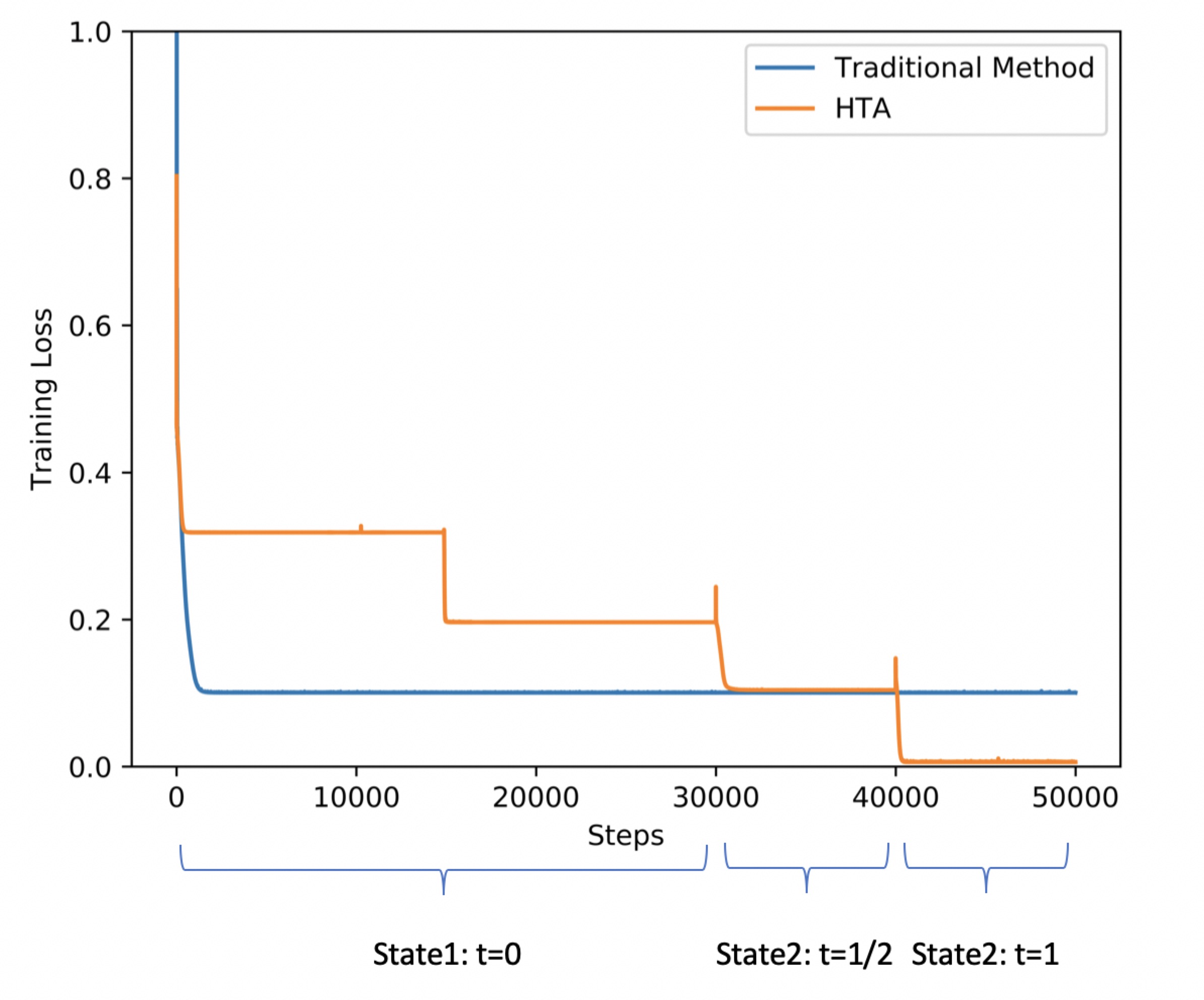
(a) Training loss

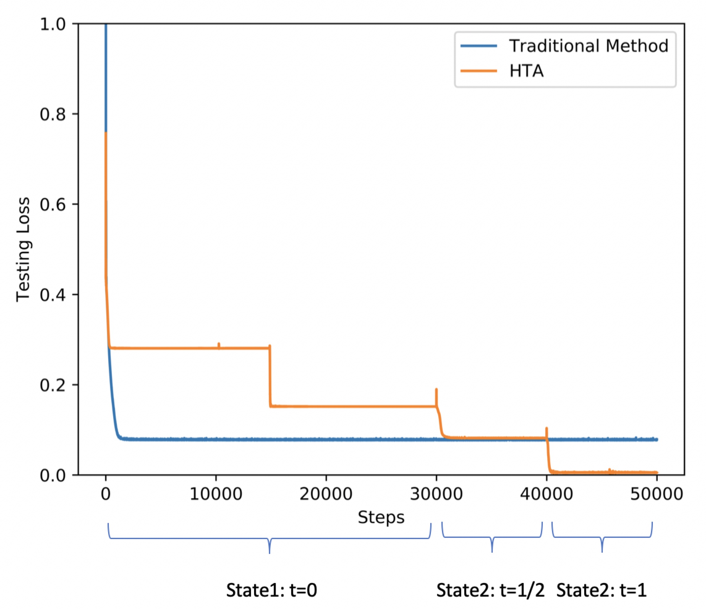
(b) Testing loss

Figure 3: Training/testing loss of approximating $\sin(x)$.

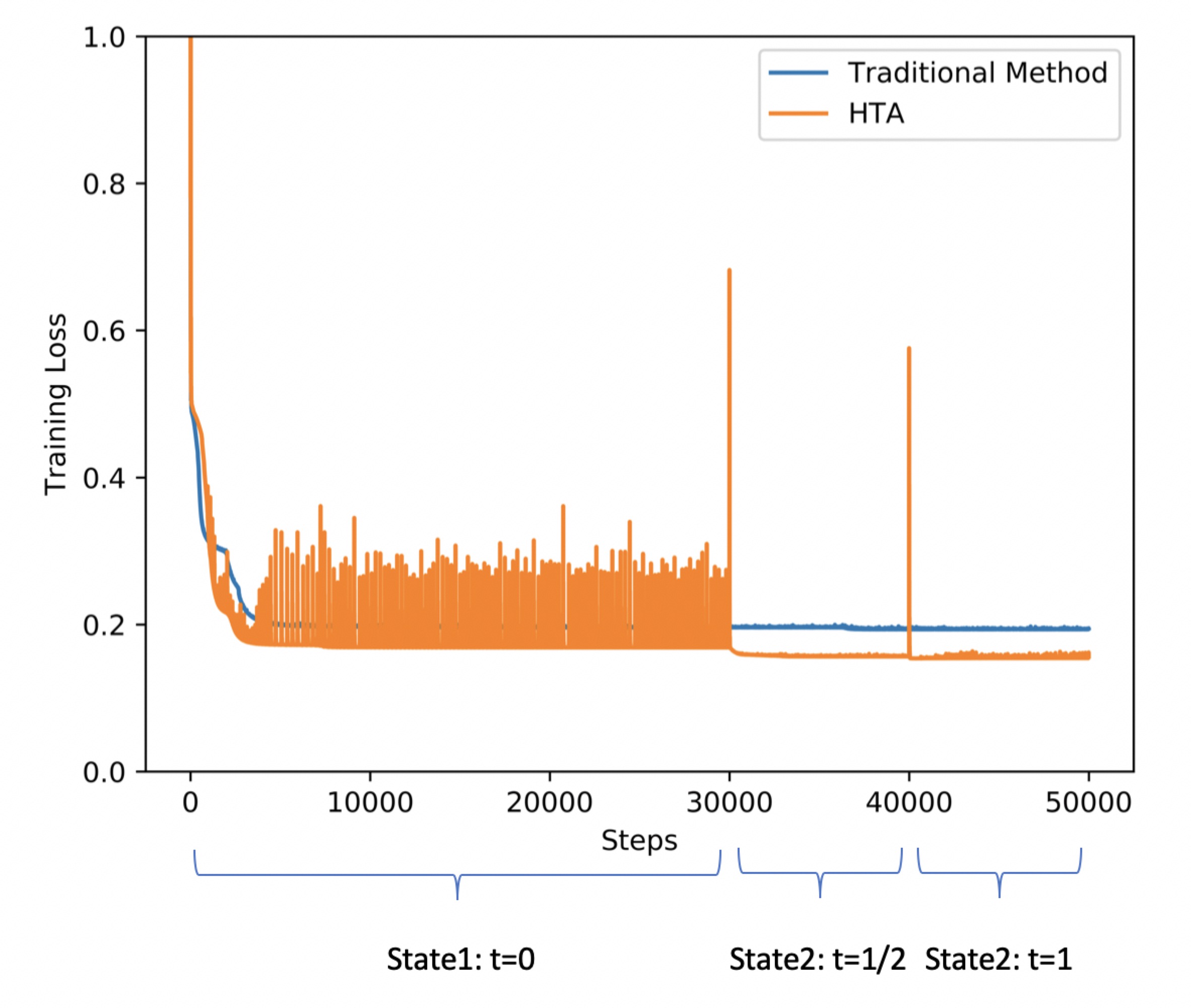
(a) Training loss

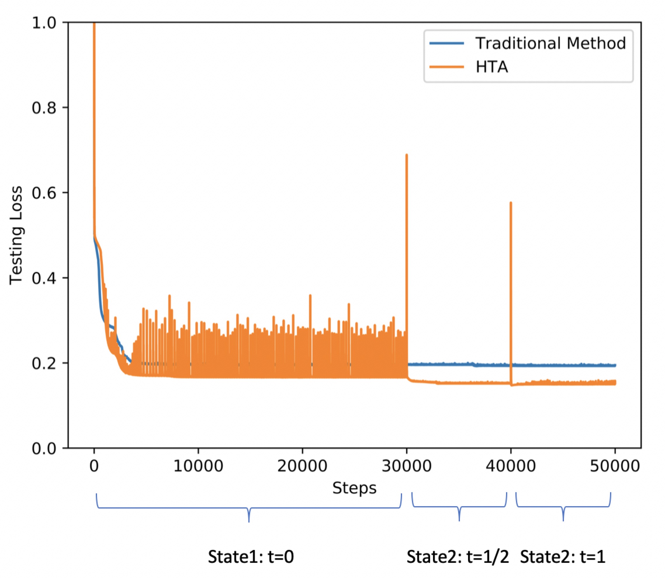
(b) Testing loss

Figure 4: Training/testing loss of approximating $\sin(x_{1}+x_{2})$.

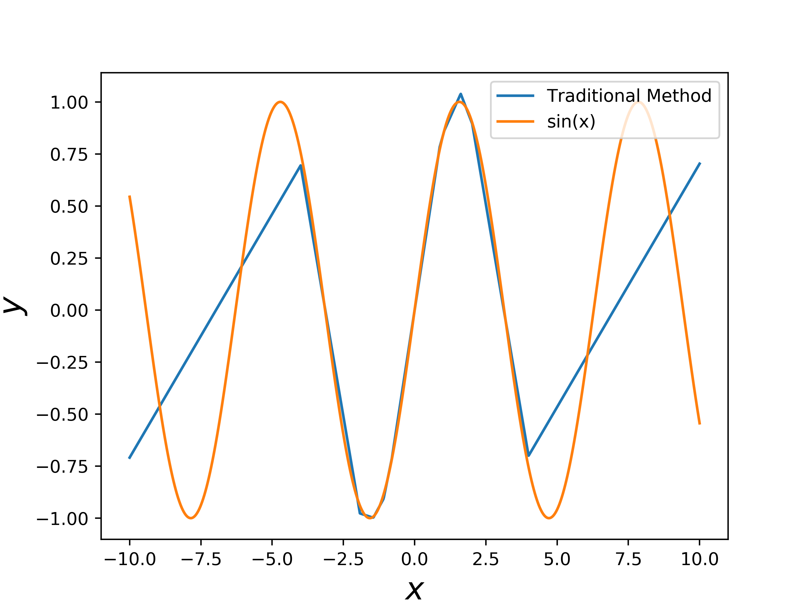
(a) Approximation results of the traditional method

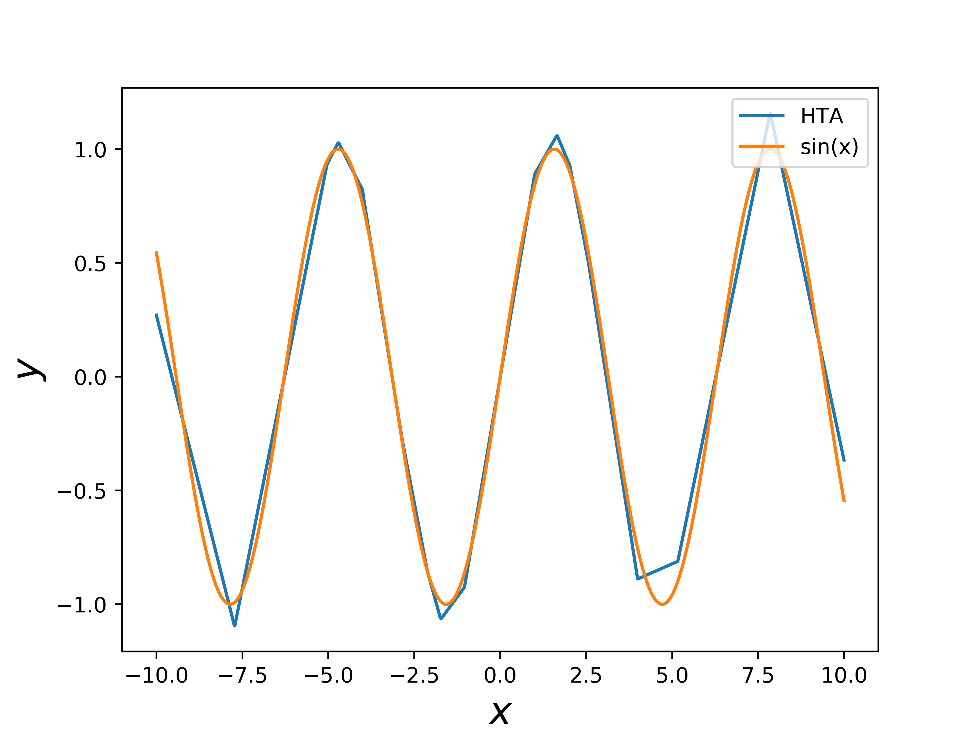
(b) Approximation results of the HTA

Figure 5: Approximation results of $\sin(x)$.

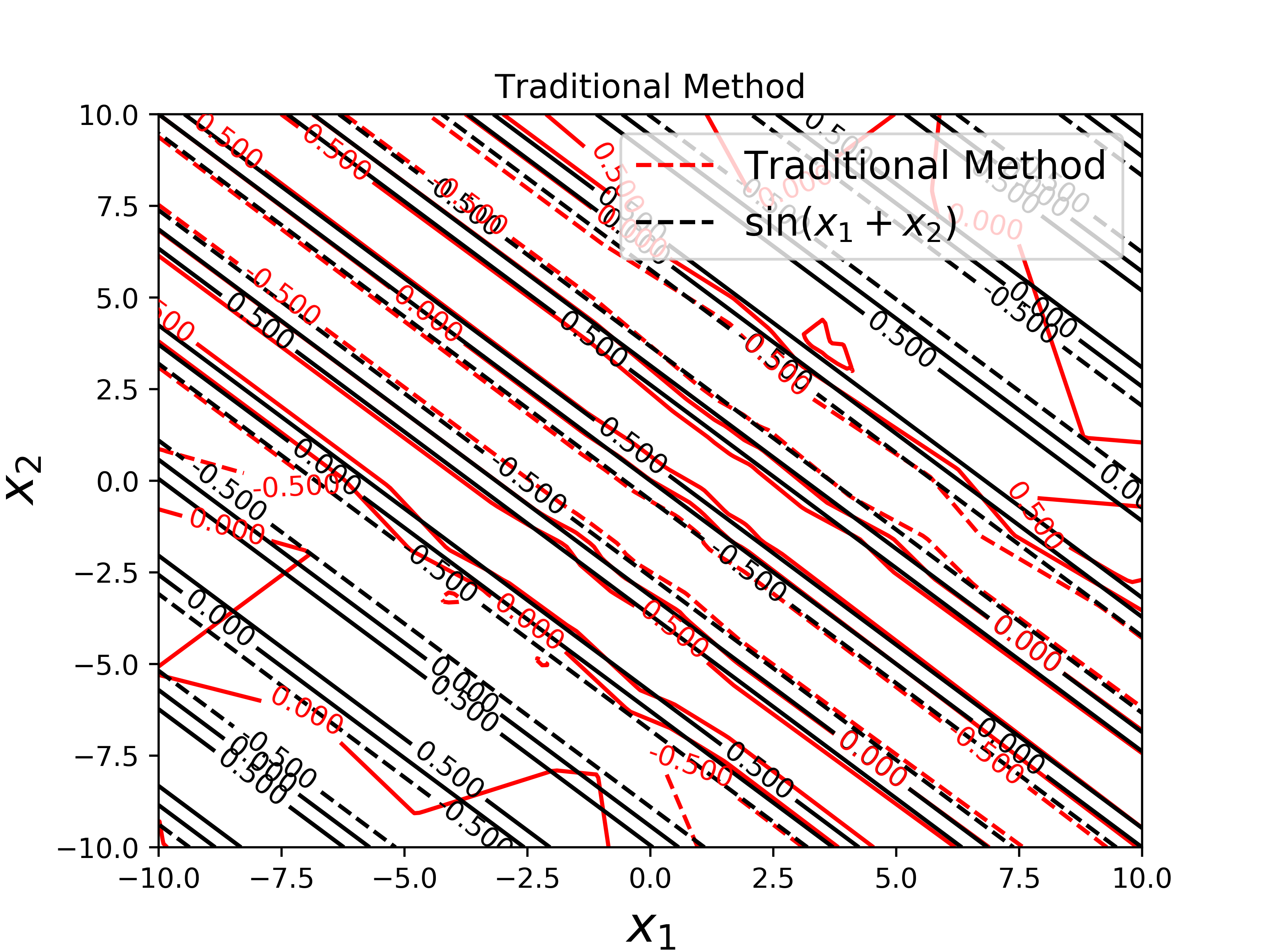
(a) Approximation results of the traditional method

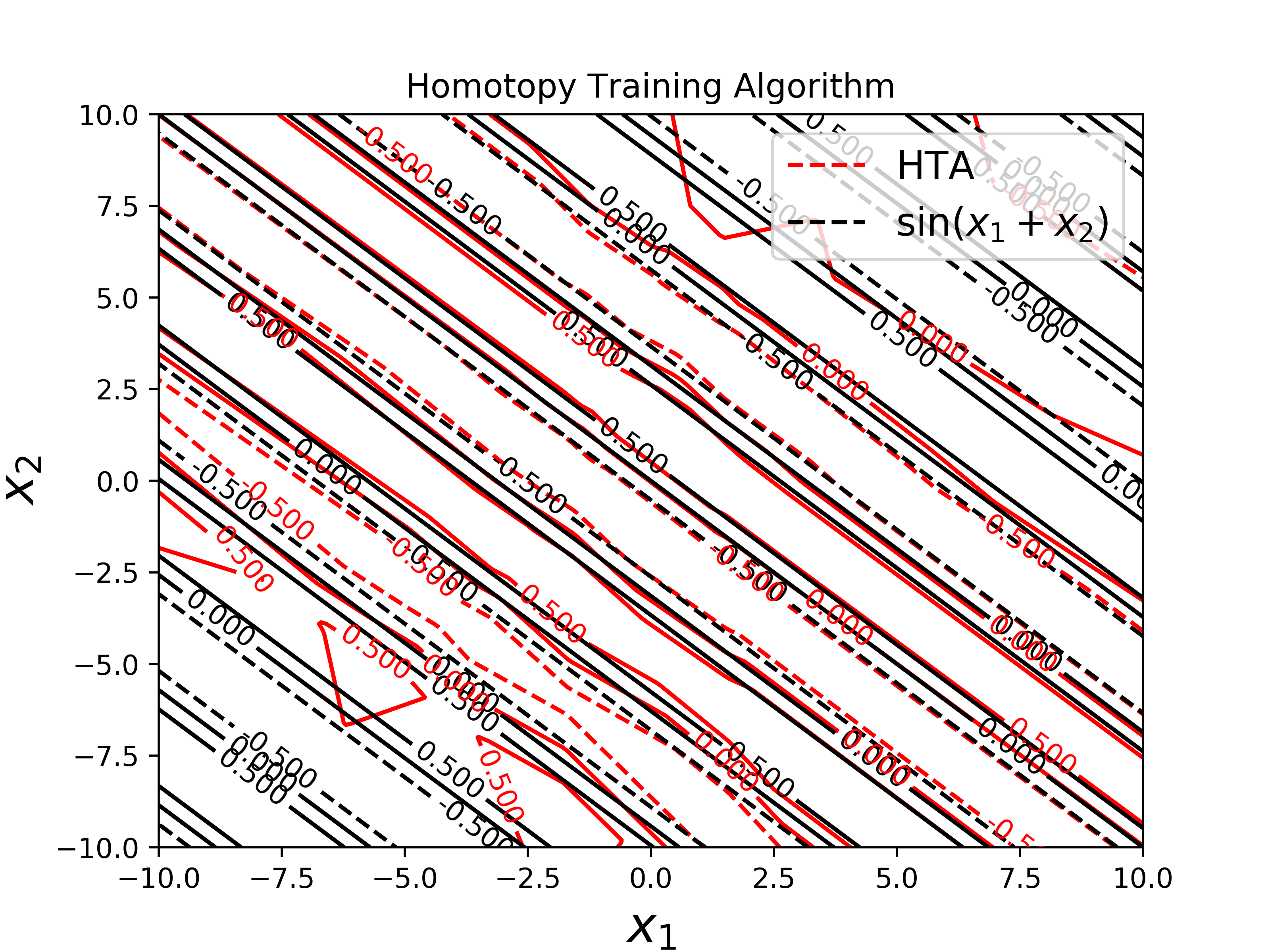
(b) Approximation results of the HTA

Figure 6: Approximation results of $\sin(x_{1}+x_{2})$.

where $x\in\mathbb{R}^{n\times 1}$, $W_{11}\in\mathbb{R}^{10\times n}$, $b_{11}\in\mathbb{R}^{10\times 1}$, $W_{21}\in\mathbb{R}^{1\times 10}$, $b_{21}\in\mathbb{R}^{1\times 1}$, $W_{1}=\left(\begin{aligned} W_{11}\\ W_{12}\\ \end{aligned}\right)\in\mathbb{R}^{20\times n}$, $b_{1}=\left(\begin{aligned} b_{11}\\ b_{12}\\ \end{aligned}\right)\in\mathbb{R}^{20\times 1}$, and $W_{2}=\left(W_{21},W_{22}\right)\in\mathbb{R}^{1\times 20}$. We use the ReLU function $r(x)=\max\{0,x\}$ as our activation function. For $n\leq 3$, we used the uniform grid points, where the sample points are the Cartesian products of uniformly sampled points of each dimension. Then the size of the training data set is $10^{2n}$. For $n\geq 4$, we employed the sparse grid [11, 41] with level 6 as sample points. For each $n$, $90\%$ of the data set is used for training while $10\%$ is used for testing. The loss curves of one-dimensional and two-dimensional cases are shown in Figs. 3 and 4. By choosing $\Delta t=0.5$, the testing loss of HTA (for $t=1$) is lower than that of the traditional training algorithm. Fig. 5 shows the comparison between the traditional method and HTA for for the one-dimensional case while Fig. 6 shows the comparison of the two-dimensional case by using contour curves. All the results of up to $n=5$ are summarized in Table 1, which lists the test loss between the HTA and the traditional training algorithm. It shows clearly that the HTA method is more efficient than the traditional method.

Example 2 (multiple hidden layers): The second example is using a two-hidden-layer fully connected neural network to approximate the same function in Example 1 for the multi-dimensional case. Since the approximation of the neutral network with a single hidden layer is not effective for $n>3$ (see Table 1), we use a two-hidden-layer fully connected neural network with 20 nodes for each layer. Then we use the following homotopy setup to increase the width of each layer from 10 to 20:

$$H_{1}(x;\theta,t)=(1-t)y_{1}(x;\theta)+ty_{2}(x;\theta),\quad H_{2}(x;\theta,t)=(1-t)y_{2}(x;\theta)+ty_{3}(x;\theta),$$ (43)

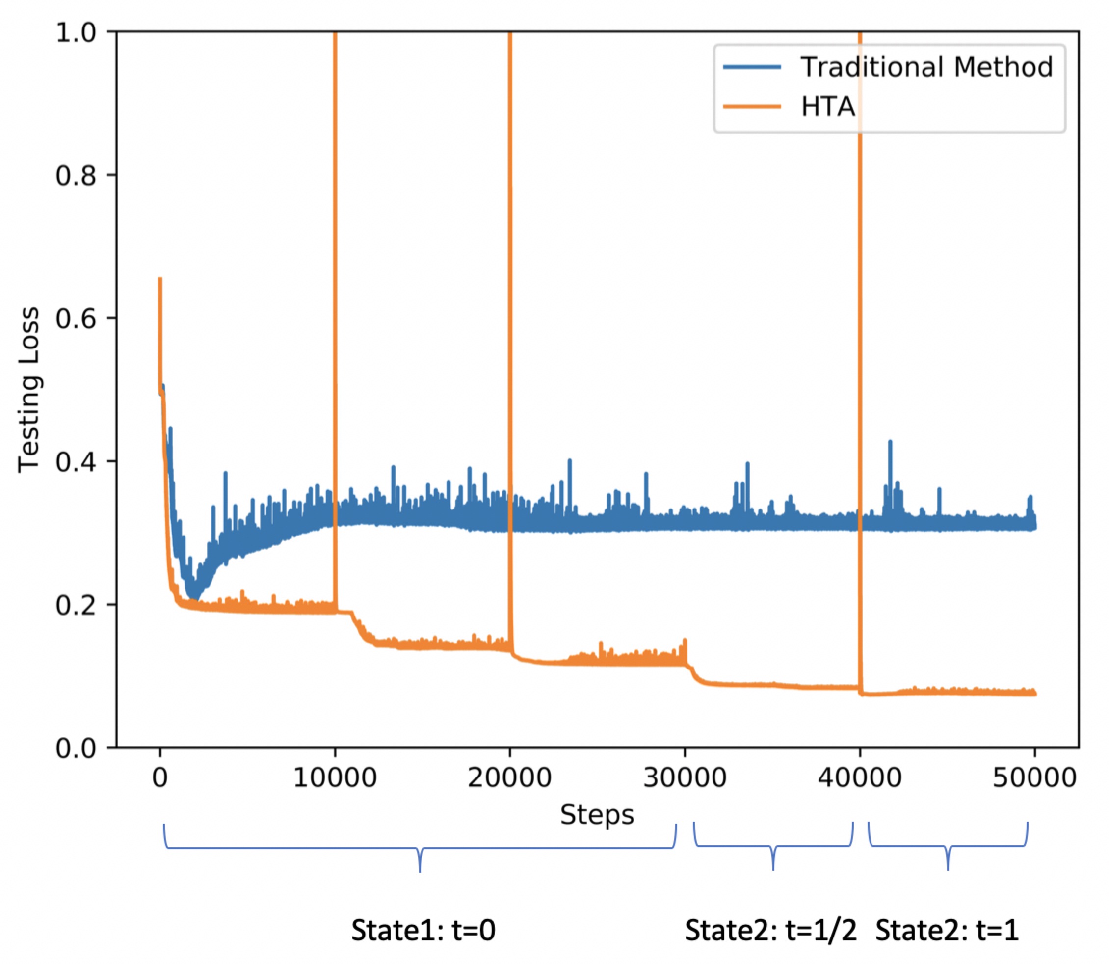
(a) Testing loss of $n=5$

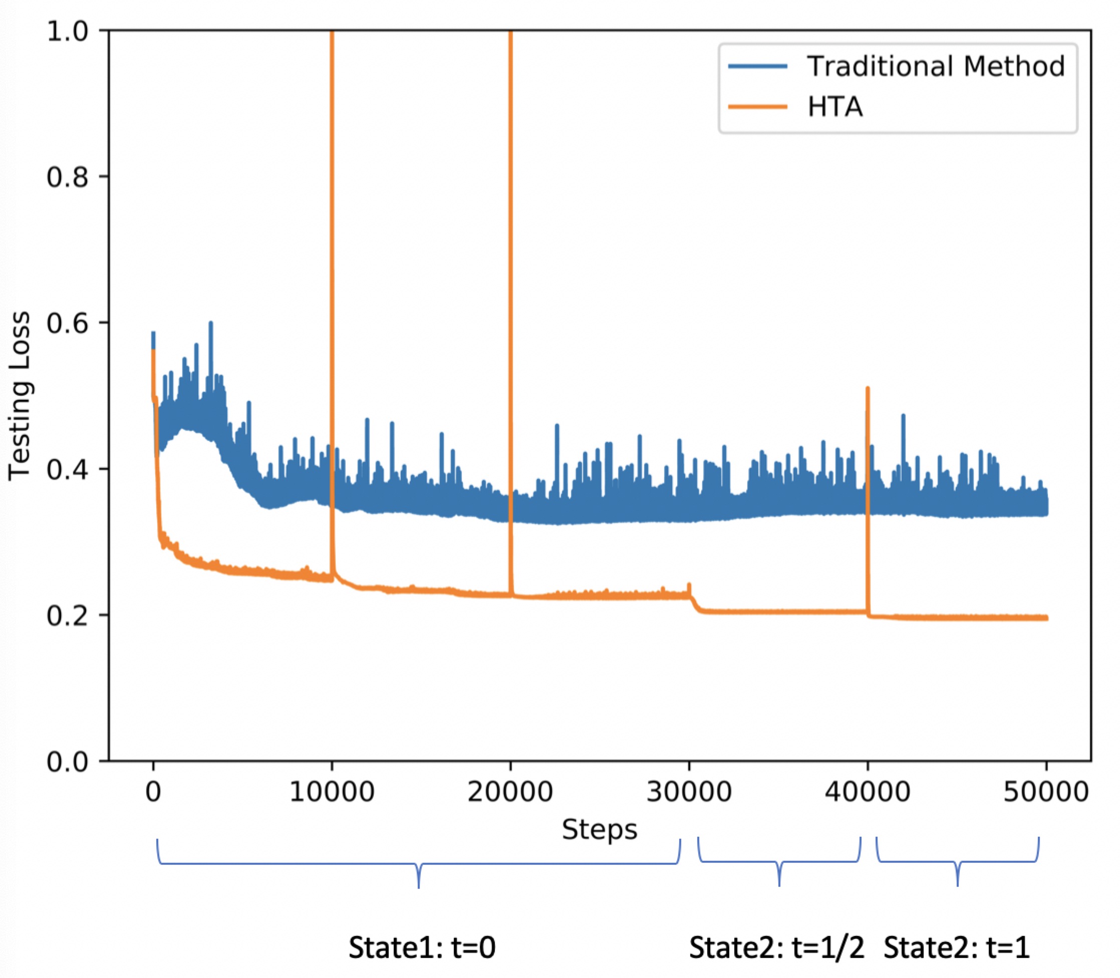
(b) Testing loss of $n=6$

Figure 7: Testing loss of approximating $\sin(x_{1}+x_{2}+\cdots+x_{n})$.

where $y_{1}$, $y_{2}$, and $y_{3}$ represent neural networks with width (10,10), (10,20), and (20,20) respectively. The rationale is that the first homotopy function, $H_{1}(x;\theta,t)$, increases the width of the first layer while the second homotopy function, $H_{2}(x;\theta,t)$, increases the width of the second layer. The size of the training data and the strategy of choosing $\Delta t$ is the same as in Example 1. Table 2 shows the results of the approximation, and Fig. 7 shows the testing curves for $n=5$ and $n=6$. The HTA achieves higher accuracy than the traditional method.

4.2 Parameter Estimation

Parameter estimation often requires a tremendous number of model evaluations to obtain the solution information on the parameter space [10, 15, 13]. However, this large number of model evaluations becomes very difficult and even impossible for large-scale computational models [25, 35]. Then a surrogate model needs to be built in order to approximate the parameter space. Neural networks provide an effective way to build the surrogate model. But an efficient training algorithm of neural networks is needed to obtain an effective approximation especially for limited sample data on parameter space. We will use the Van der Pol equation as an example to illustrate the efficiency of HTA on the parameter estimation.

Example 3: We applied the HTA to estimate the parameters of the Van der Pol equation:

$$y^{\prime\prime}-\mu(k-y^{2})y^{\prime}+y=0\hbox{~{}with~{}}y(0)=2\hbox{~{}and ~{}}y^{\prime}(0)=0.$$ (44)

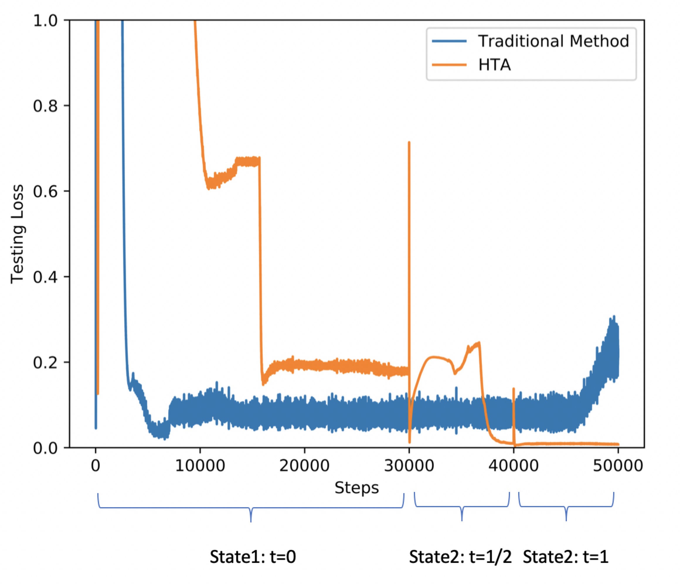
Figure 8: Testing loss of the Van der Pol equation.

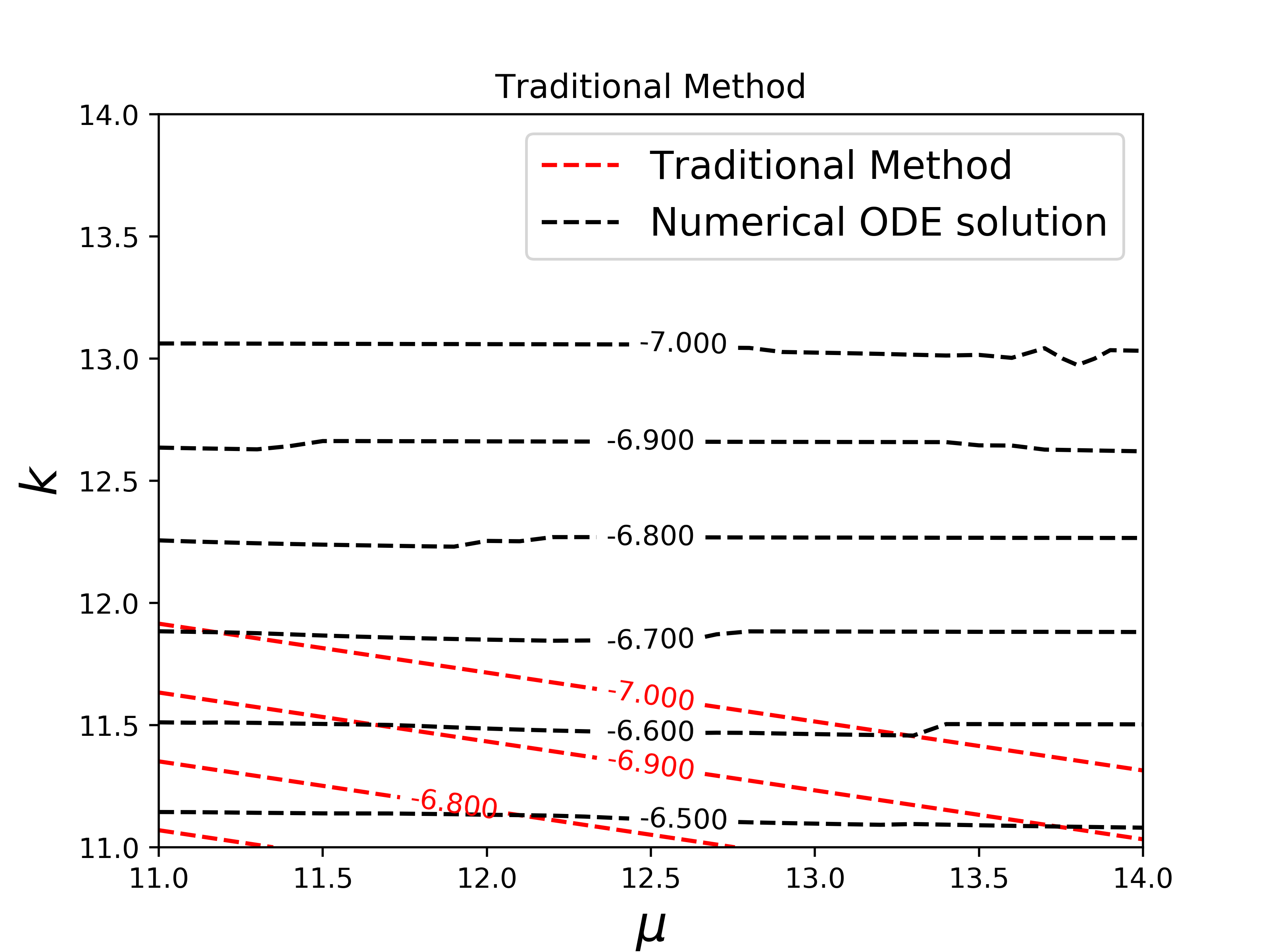
(a) The traditional method

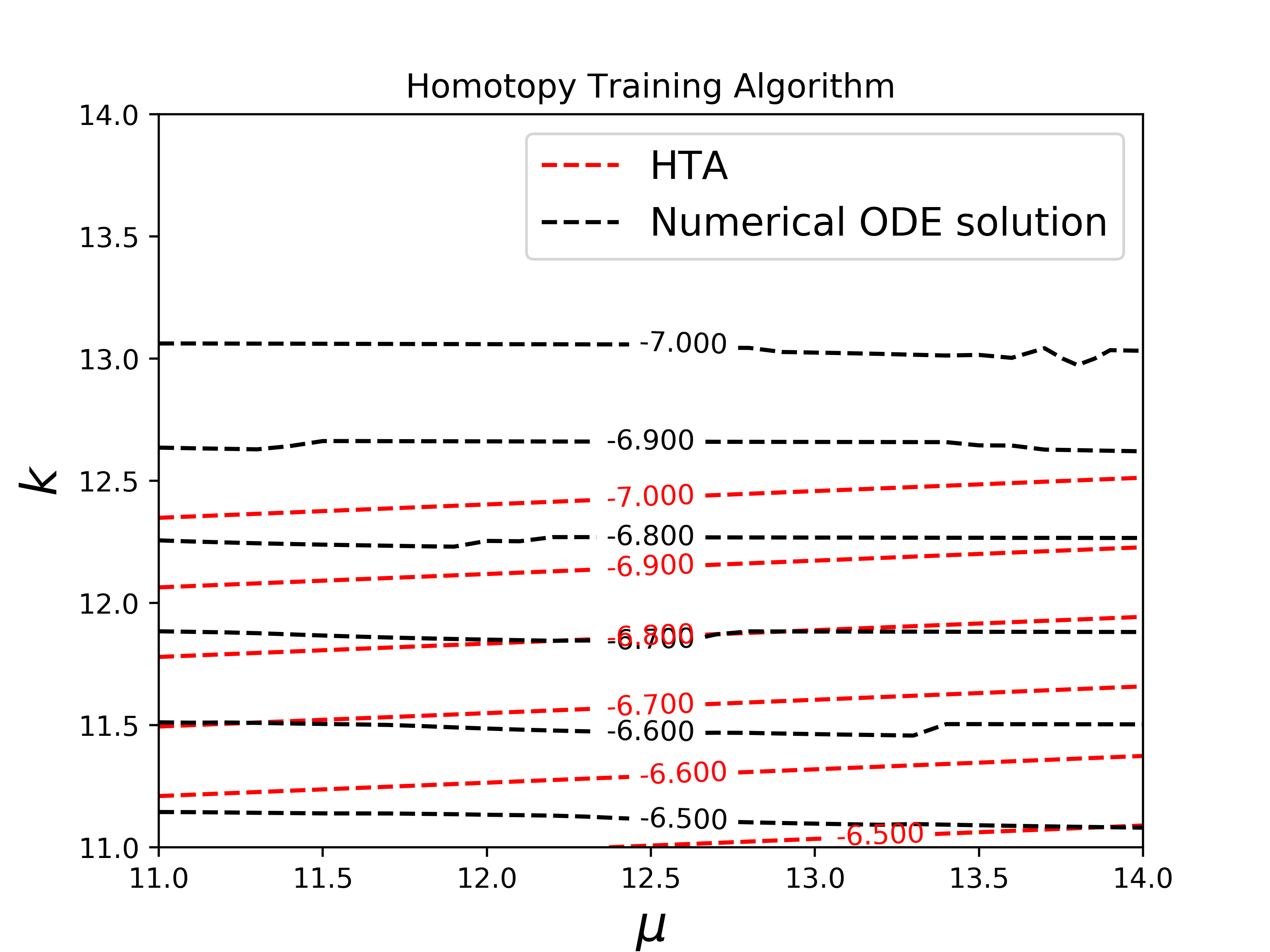
(b) The HTA

Figure 9: Comparisons between the HTA and the traditional method by contour plots of $y(1;\mu,k)$.

In order to estimate the parameters $\mu$ and $k$ for a given data $\tilde{y}(t;\mu,k)$, we first use single-hidden-layer fully connected neural network to build a surrogate model with $\mu$ and $k$ as inputs and $y(1)$ as the output. Our training data set is chosen on $1\leq\mu\leq 10$ and $1\leq k\leq 10$ with 8,281 (with $0.1$ as the mesh size). This neural network is trained by both the traditional method and the HTA. The testing dataset is 961 uniform grid points on $11\leq\mu_{i}\leq 14$ and $11\leq k_{i}\leq 14$ with $0.1$ as the mesh size for both $\mu$ and $k$ The testing loss curves of the traditional method and HTA are shown in Fig. 8: after $5\times 10^{4}$ steps, the testing loss is $0.007$ for HTA and $0.220$ for the traditional method. We also compared these two surrogate models (traditional method and HTA) with the numerical ODE solution $y(1;\mu,k)$ in Fig. 9. This comparison shows that the approximation of the HTA is closer to the ODE model than the traditional method.

Once we built surrogate models, then we moved to a parameter estimation step for any given data $\tilde{y}(t;\mu,k)$ to solve the following optimization problem

$$\min_{\mu,k}(S(\mu,k)-\tilde{y}(1))^{2},$$ (45)

where $S(\mu,k)$ is the surrogate neural network model and $\tilde{y}(1)$ is the data when $t=1$. In our example, we generated “artificial data” on the testing dataset. We use the SDG to solve the optimization problem with $\rho=k=11$ as the initial guess. We define the error of the parameter estimation below:

$$Err_{PE}=\frac{\sum_{i=1}^{n}\sqrt{(\mu^{*}_{i}-\mu_{i})^{2}+(k^{*}_{i}-k_{i})^{2}}}{n},$$ (46)

where $(\mu_{i},k_{i})$ is the sample point and $(\mu^{*}_{i},k^{*}_{i})$ is the optima of (45) for a given $\tilde{y}(1)$. Then the error of HTA is 0.71 while the error of the traditional method is 1.48. We also list some results of parameter estimation for different surrogate models in Table 3. The surrogate model created by the HTA provides smaller errors than the traditional method for parameter estimation.

5 Applications to Computer Vision

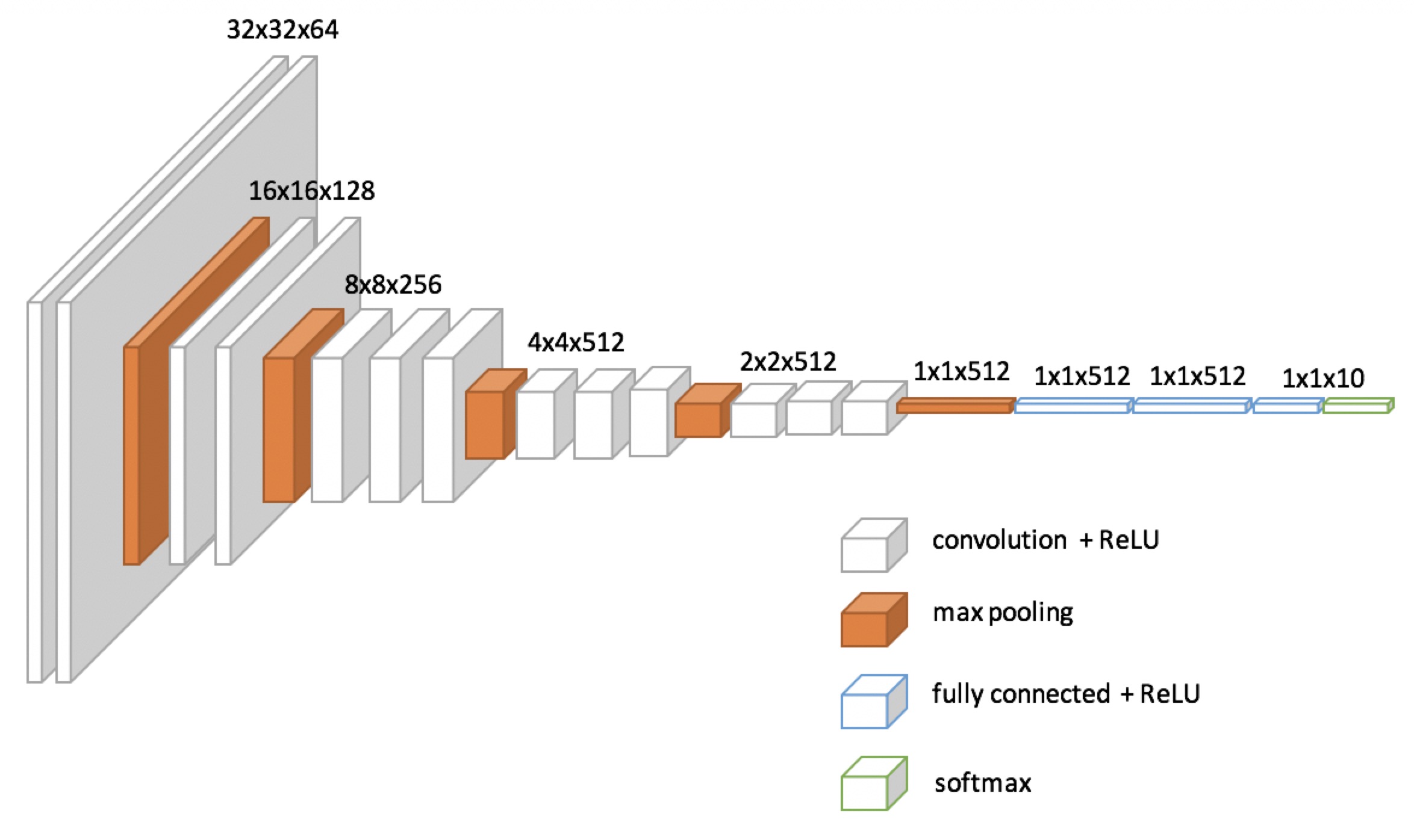
Figure 10: The structure of VGG models that consist of a convolution & pooling neural network and a fully connected neural network. The HTA is applied on the fully connected layers only.

Computer vision is one of the most common applications in the field of machine learning [32, 38]. It has diverse applications, from designing navigation systems for self-driving cars [4] to counting the number of people in a crowd [8]. There are many different models that can be used for detection and classification of objects. Since our algorithm focuses on the fully connected neural networks, we will only apply our algorithm to computer vision models with fully connected neural networks. Therefore, in this section, we will use different Visual Geometry Group (VGG) models [40] as an example to illustrate the application of HTA to computer vision. In computer vision, the VGG models use convolutional layers to extract features of the input picture, and then flatten the output tensor to be a 512-dimension-long vector. The output long vector will be sent into the fully connected network (See Fig. 10 for more details). In order to demonstrate the efficiency of HTA, we will apply it to the fully connected network part of the VGG models.

5.1 Three States of HTA

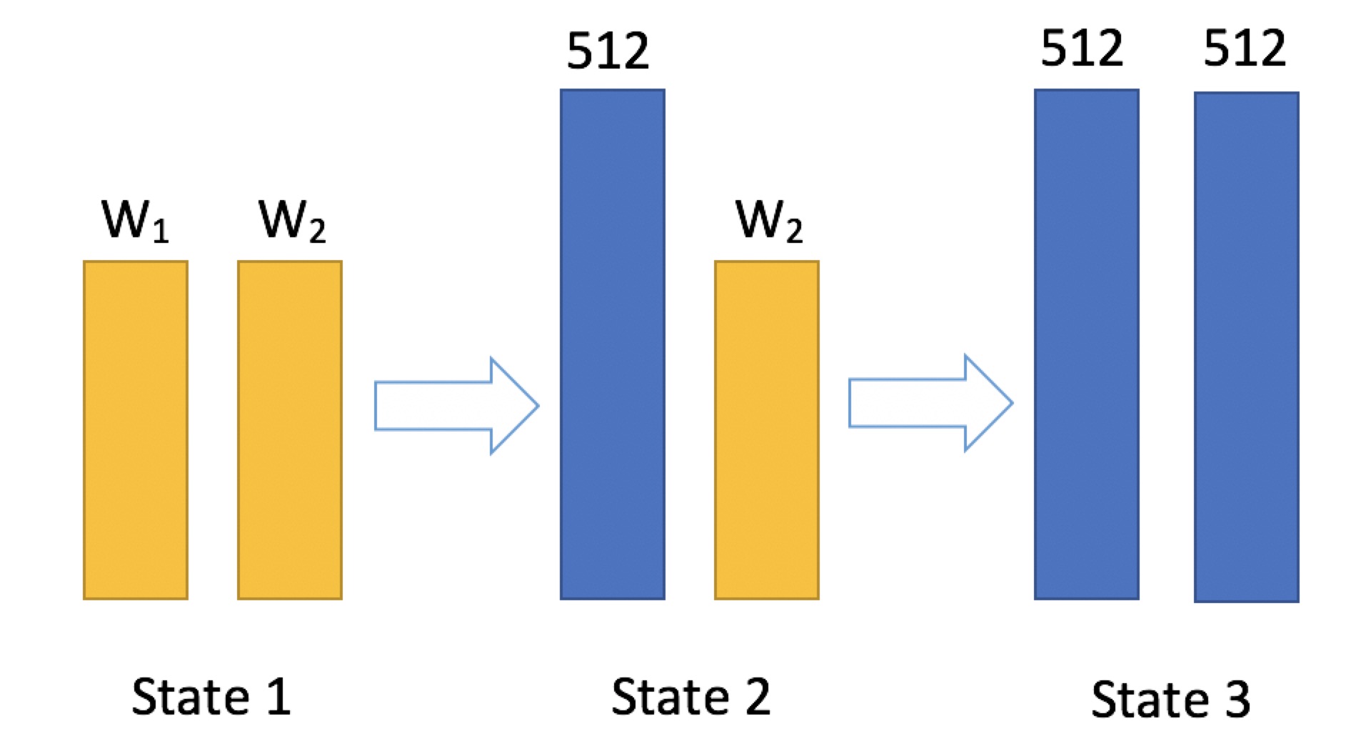
Figure 11: Three states of the VGG with the HTA.

The last stage of VGG models is a fully connected neural network that links convolutional layers of VGG to the classification categories of the Canadian Institute for Advanced Research (CIFAR-10) [31]. Then the input is the long vector generated by convolutional layers (the width is 512), while the output is the 10 classification categories of CIFAR-10. In order to train this fully connected neural network, we construct a three states setup of HTA, which is shown in Fig. 11. In this section, we use $x$ to represent the inputs generated by the convolutional layers ($x\in R^{512}$), and $\theta$ to represent the parameters for each state. The size of $\theta$ may change for different states.

• State 1: For the first state, we construct a fully connected network with 2 hidden layers. The width of the $i$-th hidden layer is set to be $w_{i}$. Then it can be written as

  $$y_{1}(x;\theta)=W_{31}\cdot r(W_{21}\cdot r(W_{11}\cdot x+b_{11})+b_{21})+b_{3},$$ (47)

  where $x\in\mathbb{R}^{512\times 1}$, $W_{11}\in\mathbb{R}^{w_{1}\times 512}$, $b_{11}\in\mathbb{R}^{w_{1}\times 1}$, $W_{21}\in\mathbb{R}^{w_{2}\times w_{1}}$, $b_{21}\in\mathbb{R}^{w_{2}\times 1}$, $W_{31}\in\mathbb{R}^{10\times w_{2}}$, and $b_{3}\in\mathbb{R}^{10\times 1}$. We use the ReLU function $r(x)=\max\{0,x\}$ as our activation function.

• State 2: For the second state, we add $(512-w_{1})$ nodes to the first hidden layer to recover the first hidden layer of the original model. Therefore, the formula of the second state becomes

  $$y_{2}(x;\theta)=W_{31}\cdot r(\tilde{W}_{2}\cdot r(W_{1}\cdot x+b_{1})+b_{21})+b_{3},$$ (48)

  where $x\in\mathbb{R}^{512\times 1}$, $W_{1}=\left(\begin{aligned} W_{11}\\ W_{12}\\ \end{aligned}\right)\in\mathbb{R}^{512\times 512}$, $b_{1}=\left(\begin{aligned} b_{11}\\ b_{12}\\ \end{aligned}\right)\in\mathbb{R}^{512\times 1}$, and $\tilde{W}_{2}=\left(W_{21},W_{22}\right)\in\mathbb{R}^{w_{2}\times 512}$. In particular, if we choose $W_{12}=0$ and $W_{22}=0$, we will recover $y_{1}(x;\theta)$ of state 1.

• State 3: Finally, we recover the original structure of the VGG by adding $(512-w_{2})$ nodes to the second hidden layer:

  $$y_{3}(x;\theta)=W_{3}\cdot r(W_{2}\cdot r(W_{1}\cdot x+b_{1})+b_{2})+b_{3},$$ (49)

  where $W_{3}=\left(\begin{aligned} W_{31},W_{32}\end{aligned}\right)\in\mathbb{R}^{10\times 512}$, $W_{2}=\left(\begin{aligned} \tilde{W}_{2}\\ \tilde{\tilde{W}}_{2}\\ \end{aligned}\right)\in\mathbb{R}^{512\times 512}$, $b_{2}=\left(\begin{aligned} b_{21}\\ b_{22}\\ \end{aligned}\right)\in\mathbb{R}^{512\times 1}$. $y_{3}(x;\theta)$ will be reduced to $y_{2}(x;\theta)$ if $\tilde{\tilde{W}}_{2}=0$ and $W_{32}=0$.

5.2 Homotopic Path

In order to connect these three states, we use two homotopic paths thats are defined by the following homotopy functions:

$$H_{i}(x;\theta,t)=(1-t)y_{i}(x;\theta)+ty_{i+1}(x;\theta),~{}i=1,2.$$ (50)

In this homotopy setup, when $t=0$, we already have an optimal solution $\theta_{i}$ for $i$-th state and want to find an optimal solution for $\theta$ for $i+1$-th state when $t=1$. By tracking $t$ from 0 to 1, we can discover a solution path $\theta(t)$ since $y_{i}(x;\theta)$ is a special form of $y_{i+1}(x;\theta)$. Then the loss functions for the homotopy setup becomes

$$L_{i}(x,y;\theta,t)=L(H_{i}(x;\theta,t),y),$$ (51)

where $L(x,y)$ is the loss function.

5.3 Training Process

We first optimize $L(y_{1}(x;\theta_{1}),y)$ for the first state. The model structure is relatively simple to solve, and it efficiently obtains a local minimum or even a global minimum for the loss function. Then the second setup is to optimize $L_{1}(x,y;\theta,t)$ by using $\theta_{1}$ as an initial condition for $t=0$. By gradually tracking parameter $t$ to $1$, we obtain an optimal solution $\theta_{2}$ of $L(y_{2}(x;\theta),y)$. The third setup is to optimize $L_{2}(x,y;\theta,t)$ by tracking $t$ from $0$ ($\theta_{2}$) to $1$. Then we obtain an optimal solution, $\theta_{3}$, of $L(y_{3}(x;\theta),y)$. Due to the continuous paths, the optimal solution $\theta_{i+1}$ of $i+1$-th state is connected to $\theta_{i}$ of the $i$-th state by the parameter $t$. In this way, we can build our complex network adaptively.

5.4 Numerical Results on CIFAR-10

We tested the HTA with the three-state setup on the CIFAR-10 dataset. We used VGG11, VGG13, VGG16, and VGG19 with batch normalization [40] as our base models. Fig. 12 shows the comparison of validation loss between HTA and the traditional method on the VGG13 model. Using the HTA with VGG13 has a lower error rate (5.14%) than the traditional method (5.82%), showing that the HTA with VGG13 improves the error rate by 11.68%. All of the results for the different models are shown in Table 4. It is clearly seen that the HTA is more accurate than the traditional method for all of the different models. For example, the HTA with VGG11 results in an error rate of 7.02% while the traditional method results in 7.83% (an improvement of 10.34%). In addition, the HTA with VGG19 has an error rate of 5.88% compared to 6.35% with the traditional model (an improvement of 7.40%), and the HTA with VGG16 has an error rate of 5.71% while the traditional method has an error rate of 6.14% (a 7.00% improvement).

5.5 The Optimal Structure of a Fully Connected Neural Network

Since the HTA builds the fully connected neural network adaptively, it also provides a way for us to find the optimal structure of the fully connected neural network; for example, we can find the number of layers and the width for each layer. We designed an algorithm to find the optimal structure based on HTA. First, we began with a minimal model; for example, in the VGG models of CIFAR-10, the minimal width of two hidden layers is 10 because of the 10 classification. Then we applied the HTA to the first hidden layer by adding “node-by-node,” and we optimized the loss function dynamically with respect to the homotopy parameter. If the optimal width of the first hidden layer was found, then the weights of new added nodes were close to zero after optimization. Then we moved to the second hidden layer and implemented the same process to train “layer-by-layer.” When the weights of the new added nodes for the second hidden layer became close to zero, we terminated the process.

Numerical results on CIFAR-10: When we applied the algorithm for finding the optimal structure to each VGG base model, we found that the results were more accurate than when we used the base model only. For VGG11 with batch normalization, we set $\delta t=1/2$ and $n_{epoch}=50$ and found the optimal structure whose widths of the first and second hidden layers are 480 and 20, respectively. The error rate with VGG11 was reduced to 7.37% while the error rate of the base model was 7.83%. In this way, our algorithm can reach higher accuracy but with a simpler structure. The rest of our experimental results for different VGG models are listed in Table 5.

6 Conclusion

In this paper, we developed a homotopy training algorithm for the fully connected neural network models. This algorithm starts from a simple neural network and adaptively grows into a fully connected neural network with a complex structure. Then the complex neural network can be trained by the HTA to attain a higher accuracy. The convergence of the HTA for each $t$ is proved for the non-convex optimization that arises from fully connected neural networks with a $C^{1}$ activation function. Then the existence of solution path $\theta(t)$ is demonstrated theoretically for the convex case although it exists numerically in the non-convex case. Several numerical examples have been used to demonstrate the efficiency and feasibility of HTA. We also proved the convergence of HTA to the local optima if the optimization problem is convex. The application of HTA to computer vision, using the fully connected part of VGG models on CIFAR-10, provides better accuracy than the traditional method. Moreover, the HTA method provides an alternative way to find the optimal structure to reduce the complexity of a neural network. In this paper, we developed the HTA for fully connected neural networks only, but we vision it as the first step in the development of HTA for general neural networks. In the future, we will design a new way to apply it to more complex neural networks such as CNN and RNN so that the HTA can speed up the training process more efficiently. Since the structures of the CNNs and RNNs are very different from fully connected neural networks, we need to redesign the homotopy objective function in order to incorporate their structures, for instance, by including the dropout technique.

7 Figures & Tables

The output for figure is:

Figure 1: The structure of a neural network with a single hidden layer.

Figure 2: The structure of a neural network with two hidden layers.

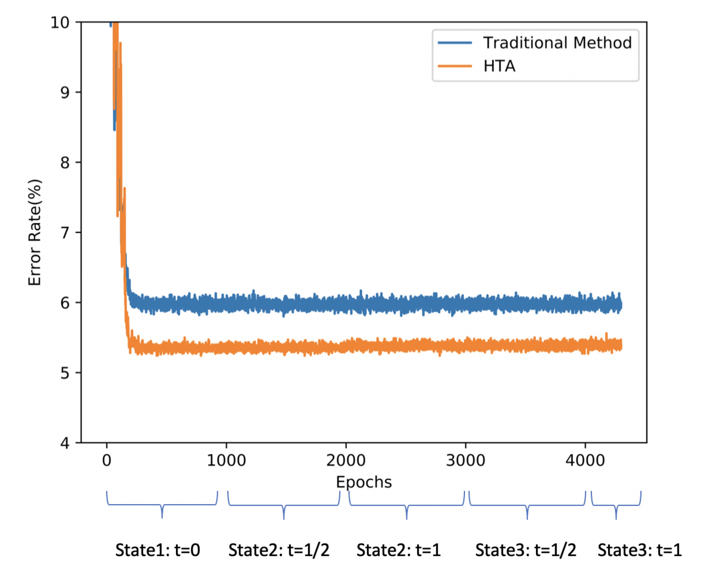
Figure 12: Comparisons of error rate for VGG13 between the HTA and the traditional method.

The output for table is:

Dimensions (n)	Test Loss	Test Loss with HTA	Number of grid points
1	$0.078$	$0.005$	$10^{2}$ (uniform grid)
2	$0.195$	$0.152$	$10^{4}$ (uniform grid)
3	$0.347$	$0.213$	$10^{6}$ (uniform grid)
4	$0.393$	$0.299$	2300 (sparse grid)
5	$0.493$	$0.352$	5503 (sparse grid)

Table 1: Testing loss of one-hidden-layer NNs.

Dimensions (n)	Test Loss	Test Loss with HTA	Number of gird points
5	$0.307$	$0.074$	5503 (sparse grid)
6	$0.340$	$0.194$	10625 (sparse grid)
7	$0.105$	$0.029$	18943 (sparse grid)
8	$0.079$	$0.022$	31745 (sparse grid)

Table 2: Testing loss of two-hidden-layer NNs.

sample points $(\mu_{i},k_{i})$	optima of traditional method $(\mu^{*}_{i},k^{*}_{i})$	optima of HTA $(\mu^{*}_{i},k^{*}_{i})$
$(11.1,12.9)$	$(11.9,11.6)$	$(11.9,12.6)$
$(11.9,13.1)$	$(11.9,11.7)$	$(11.9,12.7)$
$(12.6,11.4)$	$(11.0,11.0)$	$(12.0,11.4)$
$(13.2,12.8)$	$(11.9,11.5)$	$(11.9,12.5)$
$(13.9,11.1)$	$(11.0,11.0)$	$(12.0,11.2)$

Table 3: Parameter estimation results.

Base Model Name	Original Error Rate	Error Rate with HTA	Rate of Imrpovement(ROIs)
VGG11	$7.83\%$	$7.02\%$	$10.34\%$
VGG13	$5.82\%$	$5.14\%$	$11.68\%$
VGG16	$6.14\%$	$5.71\%$	$7.00\%$
VGG19	$6.35\%$	$5.88\%$	$7.40\%$

Table 4: The comparison between the HTA and the traditional method of VGG models on CIFAR-10

Base Model Name	Original Error Rate	Error Rate with OSF	$w_{1}$	$w_{2}$
VGG11	$7.83\%$	$7.37\%$	480	20
VGG13	$5.82\%$	$5.67\%$	980	310
VGG16	$6.14\%$	$5.91\%$	752	310
VGG19	$6.35\%$	$6.05\%$	752	310

Table 5: The results of the algorithm for finding the optimal structure when applied to CIFAR-10: $w_{i}$ stands for the optimal width of $i$-th hidden layer.

Algorithm 1 The HTA algorithm for a neural network with two hidden layers.

1:  Solve the optimization problem $\mathcal{L}(H_{1}(x;\theta,0),y$) and denote the solution as $\theta_{1}^{*}$;

2:  Set an initial guess as $\theta^{0}=\theta_{1}^{*}\cup\theta_{2}^{0}$ and $N=\frac{1}{\delta t}$ where $\delta t$ is the homotopy stepsize;

3:  for $i=1,\cdots,N$ do

4:     Solve $\theta^{i}=argmin\mathcal{L}(H_{1}(x;\theta,i\delta t),y)$ by using $\theta^{i-1}$ as the initial guess

5:  end for

References

- [1] D. Bates, J. Hauenstein, and A. Sommese. Efficient path tracking methods. Numerical Algorithms, 58(4):451–459, 2011.
- [2] D. Bates, J. Hauenstein, A. Sommese, and C. Wampler. Adaptive multiprecision path tracking. SIAM Journal on Numerical Analysis, 46(2):722–746, 2008.
- [3] M. Bernico. Deep learning quick reference: useful hacks for training and optimizing deep neural networks with TensorFlow and Keras. Packt Publishing Ltd, 2018.
- [4] M. Bojarski, D. Del Testa, D. Dworakowski, B. Firner, B. Flepp, P. Goyal, et al. End to end learning for self-driving cars. arXiv preprint arXiv:1604.07316, 2016.
- [5] L. Bottou, F. Curtis, and J. Nocedal. Optimization methods for large-scale machine learning. Siam Review, 60(2):223–311, 2018.
- [6] Z. Cang, L. Mu, and G. Wei. Representability of algebraic topology for biomolecules in machine learning based scoring and virtual screening. PLoS computational biology, 14(1):e1005929, 2018.
- [7] Z. Cang and G. Wei. Integration of element specific persistent homology and machine learning for protein-ligand binding affinity prediction. International journal for numerical methods in biomedical engineering, 34(2):e2914, 2018.
- [8] A. Chan, Z. Liang, and N. Vasconcelos. Privacy preserving crowd monitoring: Counting people without people models or tracking. In Computer Vision and Pattern Recognition, 2008. CVPR 2008. IEEE Conference on, pages 1–7. IEEE, 2008.
- [9] R. Collobert and J. Weston. A unified architecture for natural language processing: Deep neural networks with multitask learning. In Proceedings of the 25th international conference on Machine learning, pages 160–167. ACM, 2008.
- [10] A. Corbetta, A. Muntean, and K. Vafayi. Parameter estimation of social forces in pedestrian dynamics models via a probabilistic method. Mathematical biosciences and engineering, 12(2):337–356, 2015.
- [11] J. Garcke et al. Sparse grid tutorial. Mathematical Sciences Institute, Australian National University, Canberra Australia, page 7, 2006.
- [12] I. Goodfellow, Y. Bengio, and A. Courville. Deep Learning. MIT Press, 2016. http://www.deeplearningbook.org.
- [13] I. Goodman. Applications of fuzzy set theory to parameter estimation and tracking. Technical report, DTIC Document, 1983.
- [14] N. Hammerla, S. Halloran, and T. Ploetz. Deep, convolutional, and recurrent models for human activity recognition using wearables. IJCAI 2016, 2016.
- [15] W. Hao. A homotopy method for parameter estimation of nonlinear differential equations with multiple optima. Journal of Scientific Computing, 74.
- [16] W. Hao, E. Crouser, and A. Friedman. Mathematical model of sarcoidosis. Proceedings of the National Academy of Sciences, 111(45):16065–16070, 2014.
- [17] W. Hao and A. Friedman. The ldl-hdl profile determines the risk of atherosclerosis: a mathematical model. PloS one, 9(3):e90497, 2014.
- [18] W. Hao and J. Harlim. An equation-by-equation method for solving the multidimensional moment constrained maximum entropy problem. Communications in Applied Mathematics and Computational Science, 13.
- [19] W. Hao, J. Hauenstein, B. Hu, Y. Liu, A. Sommese, and Y.-T. Zhang. Bifurcation for a free boundary problem modeling the growth of a tumor with a necrotic core. Nonlinear Analysis: Real World Applications, 13(2):694–709, 2012.
- [20] W. Hao, J. Hauenstein, B. Hu, and A. Sommese. A three-dimensional steady-state tumor system. Applied Mathematics and Computation, 218(6):2661–2669, 2011.
- [21] W. Hao, J. Hauenstein, C.-W. Shu, A. Sommese, Z. Xu, and Y.-T. Zhang. A homotopy method based on weno schemes for solving steady state problems of hyperbolic conservation laws. Journal of Computational Physics, 250:332–346, 2013.
- [22] W. Hao, R. Nepomechie, and A. Sommese. Singular solutions, repeated roots and completeness for higher-spin chains. Journal of Statistical Mechanics: Theory and Experiment, 2014(3):P03024, 2014.
- [23] W. Hao, Rafael I Nepomechie, and A. Sommese. Singular solutions, repeated roots and completeness for higher-spin chains. Journal of Statistical Mechanics: Theory and Experiment, 2014(3):P03024, 2014.
- [24] W. Hao and Y. Yang. Convergence of a homotopy finite element method for computing steady states of burgers’ equation. ESAIM: Mathematical Modelling and Numerical Analysis, page to appear, 2018.
- [25] K. Haven, A. Majda, and R. Abramov. Quantifying predictability through information theory: small sample estimation in a non-gaussian framework. Journal of Computational Physics, 206(1):334–362, 2005.
- [26] K. He, X. Zhang, S. Ren, and J. Sun. Deep residual learning for image recognition. In Proceedings of the IEEE conference on computer vision and pattern recognition, pages 770–778, 2016.
- [27] K. Hornik, M. Stinchcombe, and H. White. Multilayer feedforward networks are universal approximators. Neural networks, 2(5):359–366, 1989.
- [28] G. Huang, L. Chen, C. Siew, et al. Universal approximation using incremental constructive feedforward networks with random hidden nodes. IEEE Trans. Neural Networks, 17(4):879–892, 2006.
- [29] J. Jensen. Sur les fonctions convexes et les inégalités entre les valeurs moyennes. Acta mathematica, 30(1):175–193, 1906.
- [30] K. Konda, A. Königs, H. Schulz, and D. Schulz. Real time interaction with mobile robots using hand gestures. In Proceedings of the seventh annual ACM/IEEE international conference on Human-Robot Interaction, pages 177–178. ACM, 2012.
- [31] A. Krizhevsky and G. Hinton. Learning multiple layers of features from tiny images. Technical report, Citeseer, 2009.
- [32] A. Krizhevsky, I. Sutskever, and G. Hinton. Imagenet classification with deep convolutional neural networks. In Advances in neural information processing systems, pages 1097–1105, 2012.
- [33] F. Maire, L. Mejias, and A. Hodgson. A convolutional neural network for automatic analysis of aerial imagery. In Digital lmage Computing: Techniques and Applications (DlCTA), 2014 International Conference on, pages 1–8. IEEE, 2014.
- [34] J. Markoff. A learning advance in artificial intelligence rivals human abilities. New York Times, 10, 2015.
- [35] I. Masliev and L. Somlyody. Probabilistic methods for uncertainty analysis and parameter estimation for dissolved oxygen models. Water Science and Technology, 30(2):99–108, 1994.
- [36] A. Morgan and A. Sommese. Computing all solutions to polynomial systems using homotopy continuation. Applied Mathematics and Computation, 24(2):115–138, 1987.
- [37] D. Rao and B. McMahan. Natural Language Processing with PyTorch: Build Intelligent Language Applications Using Deep Learning. ” O’Reilly Media, Inc.”, 2019.
- [38] H. Rowley, S. Baluja, and T. Kanade. Neural network-based face detection. IEEE Transactions on pattern analysis and machine intelligence, 20(1):23–38, 1998.
- [39] T. Sainath, A. Mohamed, B. Kingsbury, and B. Ramabhadran. Deep convolutional neural networks for lvcsr. In Acoustics, speech and signal processing (ICASSP), 2013 IEEE international conference on, pages 8614–8618. IEEE, 2013.
- [40] K. Simonyan and A. Zisserman. Very deep convolutional networks for large-scale image recognition. Computer Science, 2014.
- [41] S.A. Smolyak. Quadrature and interpolation formulas for tensor products of certain classes of functions. In Doklady Akademii Nauk, volume 148, pages 1042–1045. Russian Academy of Sciences, 1963.
- [42] V. Vapnik. An overview of statistical learning theory. IEEE transactions on neural networks, 10(5):988–999, 1999.
- [43] Y. Wang, W. Hao, and G. Lin. Two-level spectral methods for nonlinear elliptic equations with multiple solutions. SIAM Journal on Scientific Computing, 40.
- [44] P. Yin, S. Zhang, J. Lyu, S. Osher, Y. Qi, and J. Xin. Binaryrelax: A relaxation approach for training deep neural networks with quantized weights. arXiv preprint arXiv:1801.06313, 2018.
- [45] P. Yin, S. Zhang, Y. Qi, and J. Xin. Quantization and training of low bit-width convolutional neural networks for object detection. arXiv preprint arXiv:1612.06052, 2016.