Bayesian optimization of chemical composition: a comprehensive framework and its application to $R$Fe₁₂-type magnet compounds

Abstract

We propose a framework for optimization of the chemical composition of multinary compounds with the aid of machine learning. The scheme is based on first-principles calculation using the Korringa-Kohn-Rostoker method and the coherent potential approximation (KKR-CPA). We introduce a method for integrating datasets to reduce systematic errors in a dataset, where the data are corrected using a smaller and more accurate dataset. We apply this method to values of the formation energy calculated by KKR-CPA for nonstoichiometric systems to improve them using a small dataset for stoichiometric systems obtained by the projector-augmented-wave (PAW) method. We apply our framework to optimization of $R$Fe₁₂-type magnet compounds (R_1-αZ_α)(Fe_1-βCo_β)_12-γTi_γ, and benchmark the efficiency in determination of the optimal choice of elements (R and Z) and ratio ($\alpha$, $\beta$ and $\gamma$) with respect to magnetization, Curie temperature and formation energy. We find that the optimization efficiency depends on descriptors significantly. The variable $\beta$, $\gamma$ and the number of electrons from the R and Z elements per cell are important in improving the efficiency. When the descriptor is appropriately chosen, the Bayesian optimization becomes much more efficient than random sampling.

I Introduction

Machine learning is attracting much attention these days, and its application to data obtained by first-principles calculation is a promising way to accelerate the exploration of novel materials. The basic idea is as follows: (i) introduce a numerical representation $x$ for the materials, which is called descriptor, (ii) calculate a property $y$ for materials from the search space of the descriptor by first-principles calculation, and (iii) infer a relation $y=f(x)$ between $x$ and $y$ from thus obtained data by modeling $f$. Many efforts have been made to develop models and descriptors that work in materials discovery.Rupp et al. (2012); Ghiringhelli et al. (2015); Seko et al. (2015); Pham et al. (2016); Lam Pham et al. (2017); Dam et al. (2018); Pham et al. (2018); Ouyang et al. (2018); Seko et al. (2018) These models can be used to identify promising candidates by predicting the property $f(x^{\prime})$ for unknown materials $x^{\prime}$. It is also possible to perform the modeling and the sampling alternately to obtain the optimal $x$ as quickly as possible, which is called optimization.

Bayesian optimization (BO) is a powerful technique to find the maximum (or the minimum) of an unknown function along this idea. It is based on Bayesian modeling using a dataset collected in the previous sampling–modeling iterations, and does not require explicit form of the function $y=f(x)$. This method is efficient because it takes account of the uncertainty of a model in addition to the mean value. Figure 1 illustrates a typical situation in which BO is efficient. The dashed line is the true model. Suppose we have four sampled points which are denoted by black circles. By Bayesian modeling, we obtain the mean value (solid line) and the uncertainty (gray region). In this situation, the mean value does not give good prediction for the highest-score point. However, by considering the information of the uncertainty, one can find a significant probability that the true model has the maximum between the two rightmost data points.

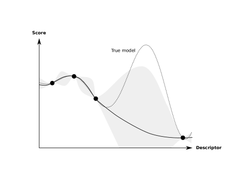
Figure 1: Schematic illustration of a typical situation in which Bayesian optimization works efficiently. The dashed line represents the true model; the black circles denote sampling points; the solid line shows a model obtained from the sampling points, and the gray region shows a confidence interval of the model.

BO has been recently applied in various problems in materials science.Ueno et al. (2016); Ju et al. (2017); Kikuchi et al. (2018) It has also a potential for application to optimization of a chemical composition,Yuan et al. (2018) but there was no reports on quantitative estimation of efficiency in such a problem avoiding possible overestimation by mere luck to our knowledge. In such applications, we need to properly choose a search space, a descriptor for the candidate systems, and a score to describe the performance that are suitable for the problem. Otherwise, the efficiency of the scheme is deteriorated. A descriptor—a form to which the input data is encoded—is especially crucial.Oganov and Valle (2009); Ghiringhelli et al. (2015); Lam Pham et al. (2017); Pham et al. (2018); Dam et al. (2018); Ouyang et al. (2018)

Accuracy of the first-principles calculation is also of great importance in the computer-aided materials search. However, conventional methods are often insufficient to achieve enough accuracy while sophisticated schemes are too much time-consuming for the purpose. For example, the magnetic transition temperature is overestimated in the mean-field approximation. Systematic errors also come in from numerical factors, such as a limited number of basis functions.

It is one of promising ideas to improve the data by using a smaller dataset from more accurate calculations or experiments.Kennedy and O’Hagan (2000); Pilania et al. (2017) This idea is also seen in the notion of transfer learning, which uses referential datasets that are different from the target dataset, and transfer the knowledge from the reference to the target.Pan et al. (2010); Hutchinson et al. (2017) However, there is no method that works for any purposes, and we need to devise a method that is suitable for each of the problems on the basis of knowledge about the origin of the error.

In this paper, we propose a practical framework for optimizing nonstoichiometric composition of multinary compounds based on Bayesian optimization and first-principles calculation. We perform a benchmark of our scheme and discuss its efficiency in the optimization using a dataset obtained by first-principles calculation with the KKR-CPA method for systems with nonstoichiometric compositions. We investigate the performance of descriptors, and discuss how we can choose an efficient one for problems. To set up a pragmatic problem, we deal with an issue from the cutting-edge of the materials study on hard magnets. We also present a method for correcting systematic errors in the formation energy by using smaller but more accurate dataset. Our idea is to construct a model of errors on the basis of our understanding of it.

This paper is organized as follows: in section II, we describe our problem setup for the benchmark, providing the background. In the first part of Section III, we present a brief summary of the whole framework. We then provide details of Bayesian optimization and the first-principles calculation in the subsequent subsections. Section III.3 is devoted to the method for integrating datasets that we use to improve the formation energy. We present the results of the benchmark and the data integration in Section IV. Finally, we conclude the paper with a summary in Section V.

II Problem setup and its background

$R$Fe₁₂-type compounds having the ThMn₁₂ structure have been considered as a possible main phase of a strong hard-magnet because they are expected to have high magnetization due to its high Fe content, and to have high magnetocrystalline anisotropy if the $R$ element is properly chosen.Ohashi et al. (1988a, b); Yang et al. (1988); Verhoef et al. (1988); De Mooij and Buschow (1988); Buschow (1988); Jaswal et al. (1990); Coehoorn (1990); Buschow (1991); Sakurada et al. (1992); Sakuma (1992); Asano et al. (1993); Akayama et al. (1994); Kuz’min et al. (1999); Gabay et al. (2016); Körner et al. (2016); Ke and Johnson (2016); Fukazawa et al. (2017, 2019) The magnetic properties of NdFe₁₂N was evaluated theoretically a few years ago Miyake et al. (2014), and its high magnetization and anisotropy field were confirmed by a successful synthesis of NdFe₁₂N_x film.Hirayama et al. (2015a, b)

Unfortunately, NdFe₁₂N and its mother compound NdFe₁₂ are thermally unstable. They cannot be synthesized as a bulk without substituting another element for a part of the Fe elements. Titanium is typical of such a stabilizing element.Yang et al. (1991a, b) Introduction of Ti, however, reduces the magnetization significantly. Co also has a potential to work as a stabilizing element according to a prediction by first-principles calculation.Harashima et al. (2016) Compared to Ti, Co is favorable in terms of magnetization. In fact, a recent experiment on Sm(Fe_0.8Co_0.2)₁₂ film showed that it has superior saturation magnetization and anisotropy field to Nd₂Fe₁₄B, the main phase of the current strongest magnet.Hirayama et al. (2017) Chemical substitution at the $R$ site also affects structural stability. Zirconium has been attracted attention as a stabilizing element at the rare-earth site.Suzuki et al. (2014); Sakuma et al. (2016); Kuno et al. (2016); Suzuki et al. (2016) Recent first-principles calculation predicted that Dy also works as a stabilizer.Harashima et al. (2018) Therefore, optimization of chemical composition of $R$Fe₁₂-type compounds in terms of stability and magnetic properties is an important issue for the development of next-generation permanent magnets.

Bearing these in mind, we set $R$Fe₁₂-type magnet compounds as target systems. Especially speaking, we optimize chemical formula of (R_1-αZ_α)(Fe_1-βCo_β)_12-γTi_γ (R = Y, Nd, Sm; Z = Zr, Dy) so that it maximizes magnetization, the Curie temperature, or minimizes the formation energy from the unary systems in the benchmark. Therefore, the problem is a combination of optimization with respect to the compositions ($\alpha$, $\beta$ and $\gamma$) and optimization with respect to the choice of elements for R and Z. We discuss the efficiency of the optimization by comparing a number of iterations required in Bayesian optimization with that in random sampling. We also study how the efficiency is affected by the choice of descriptor.

III Methods

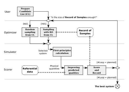
Figure 2: The workflow of the proposed scheme for materials search. The solid squares denote activities; the dashed squares with round corners represent datasets. BO stands for Bayesian optimization; CL stands for candidate list.

Figure 2 shows the workflow in our optimization framework. At the beginning of the scheme, the user prepares a list of candidate compounds. The candidates are expressed in the form of a descriptor. In this study, we prepare 11 types of descriptors for the (R_1-αZ_α)(Fe_1-βCo_β)_12-γTi_γ (R=Y, Nd, Sm; Z=Zr, Dy) systems, which we discuss in Section III.1.

Then, the candidate list is passed to the optimizer. The role of the optimizer is to pick one system from the candidate list so that a system with a high score is quickly found in the whole scheme. Because it does not have enough data to perform Bayesian optimization at the beginning, it randomly chooses a system from the list. It receives a feedback from a scorer later in the scheme, and record it. When the record reaches a certain size, the sampling method is switched to Bayesian optimization. To cover the role of the optimizer, we use a Python module called “COMmon Bayesian Optimization library” (COMBO).Ueno et al. (2016); COM We present the parameters used in our benchmark in Section III.1.

In the next stage, a quantum simulator calculates physical properties for the system chosen, which is the most time-demanding process in the scheme. The details in our simulation is described in Section III.2.

Then, the scorer integrates the calculated properties to a score. It also performs improvement of the estimated values by using the referential data before generating the score. In our application, we use the value of magnetization, Curie temperature or the formation energy as a score. As for the formation energy, we improve it by the method for integrating datasets presented in Section III.3. The preparation of the referential data is described in Section III.2. The score is fed back to the optimizer to increase the size of the data used in Bayesian optimization.

The iteration loop is repeated until the number of iterations reaches a criterion. Otherwise, the workflow goes back to the optimizer. After the loop has ended, the candidate with the best score found in the iterations is output.

III.1 Bayesian optimization

As mentioned above, we use COMBOUeno et al. (2016); COM to cover the role of the optimizer in Fig. 2. We use Thompson sampling as a heuristic to the exploration–exploitation problem in optimization. The dimension of the random feature maps, which determines the degree of approximation for the Gaussian kernel, is set to 5000. The first 10 samples are chosen randomly without using Bayesian optimization. The number of iterations is set to 100, including the first 10 iterations with the random sampling.

The candidate list consists of (R_1-αZ_α)(Fe_1-βCo_β)_12-γTi_γ systems for all the combination of R=Y, Nd, Sm; Z=Zr, Dy; $\alpha=0,0.1,\cdots,1$; $\beta=0,0.1,\cdots,1$; $\gamma=0,0.5,\cdots,2$. There are duplication in the list [e.g. YZr₀Fe₁₂ and YDy₀Fe₁₂], and the number of the unique items is 3245 out of the $3\times 2\times 11\times 11\times 5=3630$ systems.

We use 11 different sets of descriptors listed in Table 1. The descriptors consist of the number of electrons per cell ($N$), the number of electrons from the R element per cell ($N_{\mathrm{R}}$), the number of electrons from the Z element per cell ($N_{\mathrm{Z}}$), $N_{\mathrm{R}}+N_{\mathrm{Z}}$ ($\equiv N_{\mathrm{2a}}$), the number of electrons from the transition elements—namely Fe,Co,Ti—per cell ($N_{\mathrm{T}}$), the atomic number of the R element ($Z_{\mathrm{R}}$), the atomic number of the Z element ($Z_{\mathrm{Z}}$), an index for the R element ($n_{\mathrm{R}}$ = 0, 1, 2 corresponding to R = Y, Nd, Sm), an index for the Z element ($n_{\mathrm{Z}}$ = 0, 1 corresponding to Z = Zr, Dy), the Z content per cell ($\alpha$), the Co/(Fe+Co) ratio ($\beta$), the Ti content ($\gamma$), and the values of $\alpha_{1}$, $\alpha_{2}$, $\alpha_{3}$, and $\alpha_{4}$ when the chemical formula is expressed in the form of (Y${}_{1-\alpha_{1}-\alpha_{2}-\alpha_{3}-\alpha_{4}}$Nd${}_{\alpha_{1}}$Sm${}_{\alpha_{2}}$Zr${}_{\alpha_{3}}$Dy${}_{\alpha_{4}}$) (Fe_1-βCo_β)_12-γTi_γ.

Table 1: 11 Descriptors used in the Bayesian optimization. See the text for description of the variables, $N$, $N_{\mathrm{R}}$, $N_{\mathrm{Z}}$, $N_{\mathrm{2a}}$, $N_{\mathrm{T}}$, $Z_{\mathrm{R}}$, $Z_{\mathrm{Z}}$, $n_{\mathrm{R}}$, $n_{\mathrm{Z}}$, $\alpha$, $\beta$, $\gamma$, $\alpha_{1}$, $\alpha_{2}$, $\alpha_{3}$ and $\alpha_{4}$.

#1	$N$	—	—
#2	$N_{\mathrm{2a}}$, $N_{\mathrm{T}}$	#7	$N_{\mathrm{2a}}$, $\beta$, $\gamma$
#3	$N_{\mathrm{R}}$, $N_{\mathrm{Z}}$, $N_{\mathrm{T}}$	#8	$N_{\mathrm{R}}$, $N_{\mathrm{Z}}$, $\beta$, $\gamma$
#4	$Z_{\mathrm{R}}$, $Z_{\mathrm{Z}}$, $\alpha$, $N_{\mathrm{T}}$	#9	$Z_{\mathrm{R}}$, $Z_{\mathrm{Z}}$, $\alpha$, $\beta$, $\gamma$
#5	$n_{\mathrm{R}}$, $n_{\mathrm{Z}}$, $\alpha$, $N_{\mathrm{T}}$	#10	$n_{\mathrm{R}}$, $n_{\mathrm{Z}}$, $\alpha$, $\beta$, $\gamma$
#6	$\alpha_{1}$, $\alpha_{2}$, $\alpha_{3}$, $\alpha_{4}$, $N_{\mathrm{T}}$	#11	$\alpha_{1}$, $\alpha_{2}$, $\alpha_{3}$, $\alpha_{4}$, $\beta$, $\gamma$

III.2 First-principles calculation

In the “Simulator” block in Fig.2, we perform first-principles calculation based on density functional theory with the local density approximation.Hohenberg and Kohn (1964); Kohn and Sham (1965) We use the open-core approximationJensen and Mackintosh (1991); Richter (1998); Locht et al. (2016) to the f-electrons in Nd, Sm and Dy and apply the self-interaction correction.Perdew and Zunger (1981)

We assume the ThMn₁₂ structure (Fig. 3) for the (R_1-αZ_α)(Fe_1-βCo_β)_12-γTi_γ systems. The lattice parameters are determined by linear interpolation from those for RFe₁₂, RFe₁₁Ti, ZFe₁₂, ZFe₁₁Ti and RCo₁₂. These values for the stoichiometric systems were calculate with the PAW methodBlöchl (1994); Kresse and Joubert (1999) using a software package QMASQMA . We use the PBE exchange-correlation functionalPerdew et al. (1996) of the Generalized Gradient Approximation (GGA) to obtain adequate structures. The values for ZFe₁₁Ti and RCo₁₂ are presented in Appendix A. Those for RFe₁₂, RFe₁₁Ti and ZFe₁₂ are in Refs.Fukazawa et al. (2018); Harashima et al. (2015a, 2018).

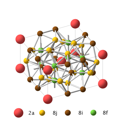
Figure 3: The 2a, 8j, 8i, and 8f Wycoff positions in the ThMn₁₂ structure. Some bonds are shown as eye-guides to see the three-dimensional structure.

In the treatment with the coherent potential approximation (CPA)Soven (1967, 1970); Shiba (1971), we assume quenched randomness for random occupation of the elements: the element R and Z are assumed to occupy the 2a site (see Fig. 3 for the Wycoff positions). Titanium is assumed to occupy the 8i site. Iron (cobalt) is assumed to occupy the 8f, 8i and 8j site with a common probability of $1-\beta$ ($\beta$) to these sites.

We calculate the magnetization, the Curie temperature, and the formation energy from the unary systems. We use the raw value of magnetization from KKR-CPA. To estimate the Curie temperature, we calculate intersite magnetic couplings by using Liechtenstein’s method,Liechtenstein et al. (1987) and convert them to the Curie temperature using the mean-field approximation.Fukazawa et al. (2018) Although this procedure overestimates the Curie temperature, we can expect from previous results that it can capture materials trend because theoretical values within the mean-field approximation had a significant correlation with experimental Curie temperatures.Fukazawa et al. (in press)

The best value among the candidates is 1.76 T [DyFe₁₂] for magnetization, 1310 K [Sm(Fe_0.2Co_0.8)₁₂] for Curie temperature, and $-2.85$ eV [SmCo₁₀Ti₂] for the formation energy. It should be noted, however, that the values on the list cannot be directly used as information for experimental synthesis because the data do not include information of phase competition (especially with Th₂Zn₁₇-type and Th₂Ni₁₇-type phases), magnetic anisotropy, and contribution to the magnetization from the f-electrons. We cover this subject in Appendix D, and provide lists of some of the best systems with the physical properties there.

As for the formation energy, KKR needs too large computational resources to obtain an accurate energy difference between systems when they have far different structures from each other. We use the method that we describe in the following subsection to correct the energy difference calculated by KKR-CPA with referential data of total energy obtained by PAW.

III.3 A method for integration datasets

Let us consider the formation energy from the unary systems defined as follows:

$$\Delta E \equiv E[\text{(R${}_{1-\alpha}$Z${}_{\alpha}$)(Fe${}_{1-\beta}$Co${}_{\beta}$)${}_{12-\gamma}$Ti${}_{\gamma}$}]$$

$$-E[\text{(the unary systems)}],$$ (1)

where “(the unary systems)” is defined as

$$(\text{the unary systems})$$

$$=(1-\alpha)\text{R}+\alpha\text{Z}$$

$$\quad+(1-\beta)(12-\gamma)\text{Fe}+\beta(12-\gamma)\text{Co}+\gamma\text{Ti},$$ (2)

and $E[\cdot]$ denotes the total energy of the system in the square bracket. Because the structures of (R_1-αZ_α)(Fe_1-βCo_β)_12-γTi_γ and each of the unary systems are much different from one another, it is not efficient to directly calculate this formation energy with the KKR method, although it can deal with non-stoichiometric systems with CPA. Our idea is to calculate the formation energy of stoichiometric systems more accurately by another method, and use calculated energies as reference data.

We construct a stochastic model for the total energy of (R_1-αZ_α)(Fe_1-βCo_β)_12-γTi_γ based on the expectation that the smaller structural difference two systems have, the more accurate energy difference KKR-CPA gives. To quantify the difference of systems, we consider a descriptor with which the difference between the systems ($\vec{x}$ and $\vec{y}$) is well-described by the distance ($|\vec{x}-\vec{y}|$). Let us denote the reference systems in the form of the descriptor by $\vec{x}^{\text{\,R}}_{1},\vec{x}^{\text{\,R}}_{2},\cdots,\vec{x}^{\text{\,R}}_{M}$ where $M$ is the number of the reference systems. The descriptor here does not have to be identical to the descriptor used in the Bayesian optimization. In the demonstration, we use a set of $(\alpha^{\prime},\beta^{\prime},\gamma^{\prime})\equiv(\alpha,\beta(12-\gamma)/12,\gamma/12)$ with which the search space can be expressed as (R${}_{1-\alpha^{\prime}}$Z${}_{\alpha^{\prime}}$)(Fe${}_{1-\beta^{\prime}-\gamma^{\prime}}$Co${}_{\beta^{\prime}}$Ti${}_{\gamma^{\prime}}$)₁₂ irrespective of the choice of the descriptor in the optimization.

For each of the reference points $\vec{x}^{\text{\,R}}_{i}$, we construct a stochastic model $\tilde{E}_{i}[\vec{y}]$ for the total energy of a system $\vec{y}$ (see also the graphs outside the box in Fig. 4):

$$\tilde{E}_{i}[\vec{y}]-E[\vec{x}^{\text{\,R}}_{i}]=E^{\prime}[\vec{y}]-E^{\prime}[\vec{x}^{\text{\,R}}_{i}]+\varepsilon_{i}.$$ (3)

The two $E$’s in the right-hand side (to which primes are attached) are the total energy calculated with KKR-CPA, whereas $E[\vec{x}^{\text{\,R}}_{i}]$ in the left-hand side is evaluated by a more accurate method, for which we use PAW in the present work. $\varepsilon_{i}$ is a random variable whose distribution is $\mathcal{N}(0,S^{2}_{i})$, i.e. the normal distribution whose mean is zero and variance is $S^{2}_{i}$, where $S^{2}_{i}\equiv\sigma^{2}\left|\vec{y}-\vec{x}^{\text{\,R}}_{i}\right|$ and $\sigma^{2}$ is a parameter we will estimate later. This model describes the expectation that the deviation of the energy difference (the first two terms in the right-hand side) from the true difference (the left-hand side) tends to be large when the difference, $\left|\vec{y}-\vec{x}^{\text{\,R}}_{i}\right|$, is large. The graphs outside the box in Fig. 4 depict how $\tilde{E}_{i}$ behave: there are three models corresponding to the three reference systems ($\vec{x}^{\mathrm{R}}_{1}$ ,$\vec{x}^{\mathrm{R}}_{2}$, $\vec{x}^{\mathrm{R}}_{3}$), and the error $\varepsilon_{i}$ in each model is large when the distance of the reference point from $\vec{y}$ is large.

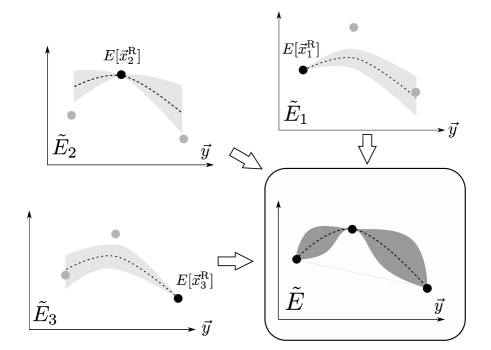
Figure 4: A schematic diagram of the procedure for constructing an integrated model. The three graphs outside the box denote the models defined by Eq. (3). They are integrated into the model described by Eq. (10).

We then integrate these models, $\tilde{E}_{1},\cdots,\tilde{E}_{M}$, into a single model $\tilde{E}$ by imposing the following condition to the distribution of $\varepsilon_{i}$:

$$\tilde{E}_{1}[\vec{y}]=\tilde{E}_{2}[\vec{y}]=\cdots=\tilde{E}_{M}[\vec{y}]\equiv\tilde{E}[\vec{y}].$$ (4)

This condition can be rewritten as follows:

$$\varepsilon_{i}=\tilde{E}[\vec{y}]-E[\vec{x}^{\text{\,R}}_{i}]-E^{\prime}[\vec{y}]+E^{\prime}[\vec{x}^{\text{\,R}}_{i}].$$ (5)

Therefore, the conditional probability distribution of $\tilde{E}$ is

$$\Pr\left(\tilde{E}[\vec{y}]=t\right)=\frac{\prod_{i}P_{i}\left(t-E[\vec{x}^{\text{\,R}}_{i}]-E^{\prime}[\vec{y}]+E^{\prime}[\vec{x}^{\text{\,R}}_{i}]\right)}{\int dt^{\prime}\prod_{i}P_{i}\left(t^{\prime}-E[\vec{x}^{\text{\,R}}_{i}]-E^{\prime}[\vec{y}]+E^{\prime}[\vec{x}^{\text{\,R}}_{i}]\right)}$$ (6)

where $P_{i}$ denotes the probability distribution function of $\mathcal{N}(0,S^{2}_{i})$. It is straightforward to see that this conditional distribution is the normal distribution whose mean $\tilde{\mu}$ and variance $\tilde{S}^{2}$ are

$$\tilde{\mu}=E^{\prime}[\vec{y}]+\frac{1}{\Omega}\sum_{i}\omega_{i}\left\{E[\vec{x}^{\text{\,R}}_{i}]-E^{\prime}[\vec{x}^{\text{\,R}}_{i}]\right\},$$ (7)

$$\tilde{S}^{2}=\frac{\sigma^{2}}{\Omega}$$ (8)

where $\omega_{i}$ is a weight and $\Omega$ is a normalization factor that are defined as

$$\omega_{i}\equiv\frac{1}{\left|\vec{y}-\vec{x}^{\text{\,R}}_{i}\right|},\quad\Omega\equiv\sum_{i}\omega_{i}.$$ (9)

In another expression, our integrated model is

$$\tilde{E}[\vec{y}]=E^{\prime}[\vec{y}]+\frac{1}{\Omega}\sum_{i}\omega_{i}\left\{E[\vec{x}^{\text{\,R}}_{i}]-E^{\prime}[\vec{x}^{\text{\,R}}_{i}]\right\}+\tilde{\varepsilon}$$ (10)

where $\tilde{\varepsilon}$ is a random variable whose distribution is $\mathcal{N}(0,\tilde{S}^{2})$. Algorithm 1 summarizes the construction of the model explained so far in a form of a pseudocode. Note that the value for the input variable $\sigma^{2}$ has not yet been determined. The characteristics of $\tilde{E}[\vec{y}]$ is illustrated in the right-bottom panel in Fig. 4. Although $\tilde{E}[\vec{y}]$ is singular at $\vec{y}=\vec{x}_{i}^{\mathrm{R}}$, it is easy to see that this is removable and $\lim_{\vec{y}\rightarrow\vec{x}_{i}^{\mathrm{R}}}\tilde{E}[\vec{y}]=E[\vec{x}_{i}^{\mathrm{R}}]$.

$\vec{x}^{\mathrm{R}}_{i}$ ($i=1,\cdots,M$), $\vec{y}\not\in\{\vec{x}^{\mathrm{R}}_{i}\}$ : descriptor; $\sigma^{2}$;

$E^{\prime}[\vec{y}]$: energy estimation; $\Delta_{i}\equiv E[\vec{x}^{\mathrm{R}}_{i}]-E^{\prime}[\vec{x}^{\mathrm{R}}_{i}]$

$\tilde{\mu}$, $\tilde{S}^{2}$

Initialize $\tilde{\mu}\leftarrow 0$, $\Omega\leftarrow 0$

for $i=1$ to $M$ do

   $\Omega\leftarrow\Omega+1/|\vec{y}-\vec{x^{\mathrm{R}}_{i}}|$

   $\tilde{\mu}\leftarrow\tilde{\mu}+\Delta_{i}/|\vec{y}-\vec{x^{\mathrm{R}}_{i}}|$

end for

Average: $\tilde{\mu}\leftarrow\tilde{\mu}/\Omega+E^{\prime}[\vec{y}]$   [Eq. (7)]

Variance: $\tilde{S}^{2}\leftarrow\sigma^{2}/\Omega$   [Eq. (8)]

Algorithm 1 A pseudocode of the algorithm for determination of $\tilde{\mu}$ in Eq.  (7) and $\tilde{S}^{2}$ in Eq. (8). This needs $\sigma^{2}$ and $\Delta_{i}$ as inputs, which are calculated by the algorithm shown in Alg. 2.

The formation energy from the unary systems can be calculated as $\Delta E\simeq\tilde{E}[\vec{y}]-E[(\text{the unary systems})]$, where $E[(\text{the unary systems})]$ is calculated by an accurate method.

To complete the formulation, we discuss estimation of $\sigma^{2}$ based on the data for the reference systems. We use the maximum likelihood estimation. However, it cannot be directly applied to our model because the distribution of $\tilde{\varepsilon}$ becomes the delta function in the limit of $\vec{y}\rightarrow\vec{x}^{\text{\,R}}_{i}$, regardless of the value of $\sigma^{2}$.

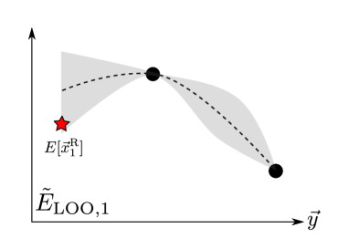
Figure 5: A schematic plot of $\tilde{E}_{\text{LOO},i}$ for $i=1$ and $M=3$.

To avoid this singularity, we consider a model $\tilde{E}_{\text{LOO},i}$ that is constructed from all reference systems but $\vec{x}^{\text{\,R}}_{i}$. Figure 5 depicts the construction of such a model. Now, we consider the probability of $\tilde{E}_{\text{LOO},i}[\vec{y}]$ at $\vec{y}=\vec{x}^{\text{\,R}}_{i}$. Regarding the probability for $\tilde{E}_{\text{LOO},i}[\vec{y}=\vec{x}^{\text{\,R}}_{i}]=E[\vec{x}^{\text{\,R}}_{i}]$ as a likelihood $L_{i}$, we select the value of $\sigma^{2}$ that maximizes $\mathcal{L}=\prod_{i}L_{i}$. We then obtain

$$\sigma^{2}=\frac{1}{M}\sum_{i}\Omega_{\text{LOO},i}\left(E[\vec{x}^{\text{\,R}}_{i}]-E^{\prime}[\vec{x}^{\text{\,R}}_{i}]\right)^{2}$$ (11)

where

$$\Omega_{\text{LOO},i}\equiv\sum_{j\neq i}\frac{1}{\left|\vec{x}^{\text{\,R}}_{i}-\vec{x}^{\text{\,R}}_{j}\right|}.$$ (12)

The determination of $\sigma^{2}$ is summarized in a form of a pseudocode in Alg. 2. The output values of $\sigma^{2}$ and $\Delta_{i}$ corresponds to those in the algorithm described in Alg. 1.

$\vec{x}^{\mathrm{R}}_{i}$ ($i=1,\cdots,M$): descriptor;

$E[\vec{x}^{\mathrm{R}}_{i}]$, $E^{\prime}[\vec{x}^{\mathrm{R}}_{i}]$: energy estimation

$\Delta_{i}$($i=1,\cdots,M$), $\sigma^{2}$

Initialize $\sigma^{2}\leftarrow 0$

for $i=1$ to $M$ do

   $\Delta_{i}\leftarrow E[\vec{x}^{\mathrm{R}}_{i}]-E^{\prime}[\vec{x}^{\mathrm{R}}_{i}]$

   $\sigma^{2}\leftarrow\sigma^{2}+\Delta_{i}^{2}\cdot\sum_{j\neq i}1/|\vec{x}^{\mathrm{R}}_{i}-\vec{x}^{\mathrm{R}}_{j}|$

end for

$\sigma^{2}\leftarrow\sigma^{2}/M$   [Eq. (11)]

Algorithm 2 A pseudocode of the algorithm for determination of $\sigma^{2}$ in Eq. (8). The energy difference $\Delta_{i}$ is also output to be used in the algorithm described in Alg. 1.

In the actual application, we calculate $E^{\prime}[\vec{x}^{\text{\,R}}_{i}]$ with the KKR-LDA method and $E[\vec{x}^{\text{\,R}}_{i}]$ with the PAW-GGA method. We need to calibrate $E[\vec{x}^{\text{\,R}}_{i}]$ with a linear term because the difference in the treatment of the core electrons is another major source of error in the total energy, which is described well by a linear function. We deal with it by extending our model to include an adjustable linear term, and use it in the actual calculation. We discuss this extension of the model in Appendix B.

IV Results and Discussion

IV.1 Integration method

We show how the integration model explained in Section III.3 works before we present the benchmark of the whole scheme in the next subsection. Let us take a simple example first: we consider a one dimensional function $E[x]=\sin(\pi x)$ as a true model. Assume that we have many data about $E^{\prime}[x]$, which is an approximate function and actually obey $E^{\prime}[x]=\sin(\pi x)+2x$. Because their derivatives differ from each other by 2, the difference $E^{\prime}[x]-E^{\prime}[x^{\text{R}}_{i}]$ deviates from $E[x]-E[x^{\text{R}}_{i}]$ roughly by $2(x-x^{\text{R}}_{i})$. The assumption of the model described in Section III.3 was that the error in $E^{\prime}[x]$ is large when $|x-x^{\text{R}}_{i}|$ is large. This is correct in the magnitude of the errors, but there is a bias in its sign. In this example, we prepare a dataset of $E^{\prime}[x]$ for $x=-0.5$ to $0.5$ with an interval of 0.02. We choose five reference points $x^{\text{R}}_{i}$ ($i=1,\cdots,5$) from the $x$-values, and prepare a dataset of $E[x^{\text{R}}_{i}]$.

The result of the prediction is shown in Fig. 6. The original points of $E^{\prime}[x]$ are shown as points in cyan. The purple points show the mean value of the model; the light purple region shows the values of the standard deviation. The green curve shows $E[x]$, the true model, and the green circles are the reference points used in the prediction.

The mean values, which may be used as values of a point estimation, are improved from the original data in most of the region. The error region also covers the line of the true model except in the region $x>0.26$.

It is noteworthy that the bias in the sign of the error mentioned above makes the uncertainty of the model large. This would be improved if we assume an asymmetric distribution for $\varepsilon_{i}$ in Eq. (3). However, the resultant form of the integrated model becomes more complicated.

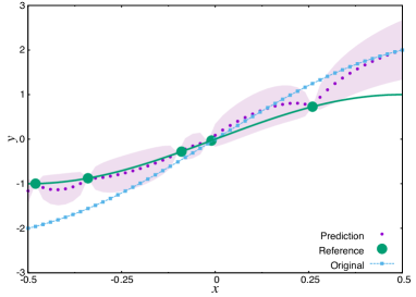
Figure 6: Results of the integration scheme when $E[x]=\sin(\pi x)$ (Green line) and $E^{\prime}[x]=\sin(\pi x)+2x$ (cyan points). The green circle denote the points of references, $E[x_{i}^{\text{R}}]$. The mean value of the improved model, $\tilde{E}[x]$, is denoted by the purple points. The standard deviation is denoted by the region in light purple.

Next, let us see the results of the formation energy obtained by this method. Figure 7 shows the formation energy of (Sm_1-αZr_α) (Fe_1-βCo_β)_12-γTi_γ from the unary systems for $\gamma=0$ (left) and $\gamma=0.5$ (right). The mean values are shown in the top two figures, and the standard deviations are shown in the bottom two figures. In each figures, the horizontal axes show values of the Co/(Fe+Co) ratio ($\beta$), and the vertical axes show values of the Zr concentration ($\alpha$).

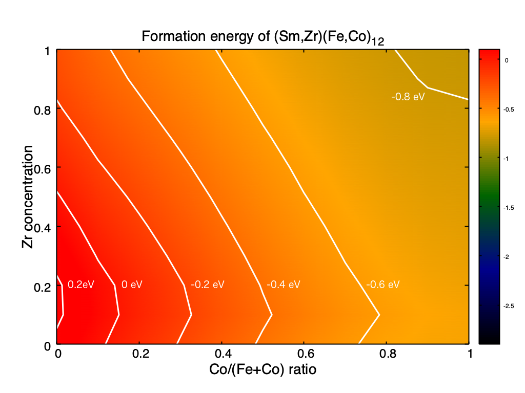
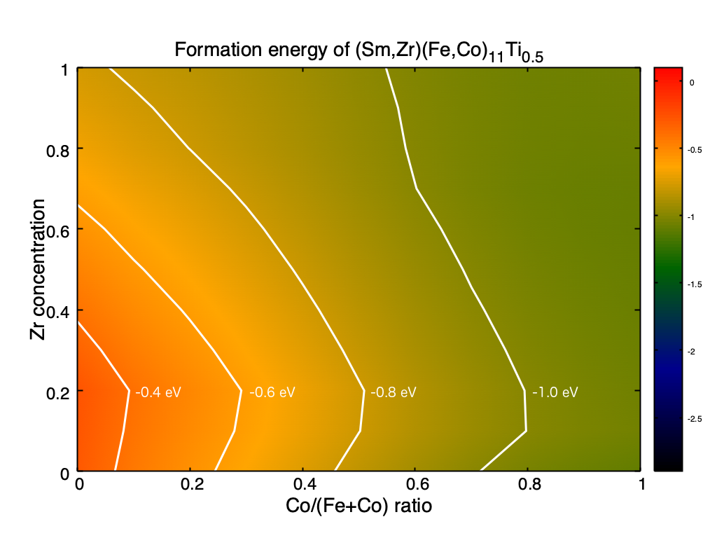
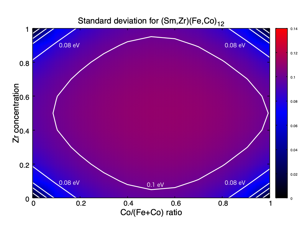
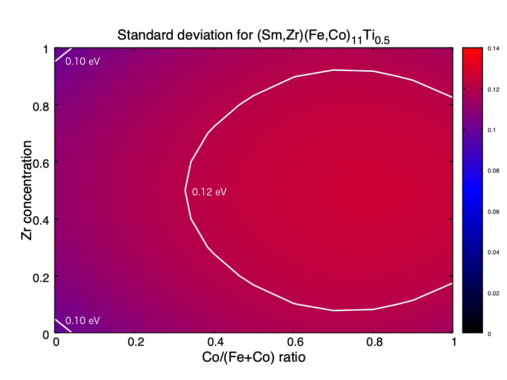
Figure 7: The mean values (top) and the standard deviations (bottom) of the integrated model for Sm(Fe,Co)₁₂ (left) and Sm(Fe,Co)_11.5Ti_0.5 (right). The intervals of the contours are 0.2 eV for the mean values and 0.02 eV for the standard deviations.

The standard deviation of the model is zero at the corners of the figure in $\gamma=0$ (left bottom) because they correspond to the reference points, namely SmFe₁₂, ZrFe₁₂, SmCo₁₂ and ZrCo₁₂. Therefore, the mean values at the corners of the left top figure are identical with the reference data (obtained by PAW-GGA). Because the other reference points are SmFe₁₁Ti and ZrFe₁₁Ti (both at $\beta=0$, $\gamma=1$), the contours are placed slightly to the right in $\gamma=0$. This is more obvious in the plot for $\gamma=0.5$ (the right bottom panel).

Although we used the mean values ($\tilde{\mu}$) in the Bayesian optimization in Section IV.2, it is important to check how the model has uncertainty in its prediction, which is typically represented by the standard deviation $\tilde{S}$: the model needs more reference points when $\tilde{S}$ is too large compared with the value of $\tilde{\mu}$. One can also make use of the upper (lower) confidence bound $\tilde{\mu}+k\tilde{S}$ ($\tilde{\mu}-k\tilde{S}$) —where $k$ is a positive adjustable parameter— instead of $\tilde{\mu}$ to take account of the uncertainty in a pessimistic (optimistic) manner.

IV.2 Bayesian Optimization

In this subsection, we show the performance of the Bayesian optimization and discuss the results. Figure 8 shows one of the optimization processes with respect to magnetization using the descriptor #8.

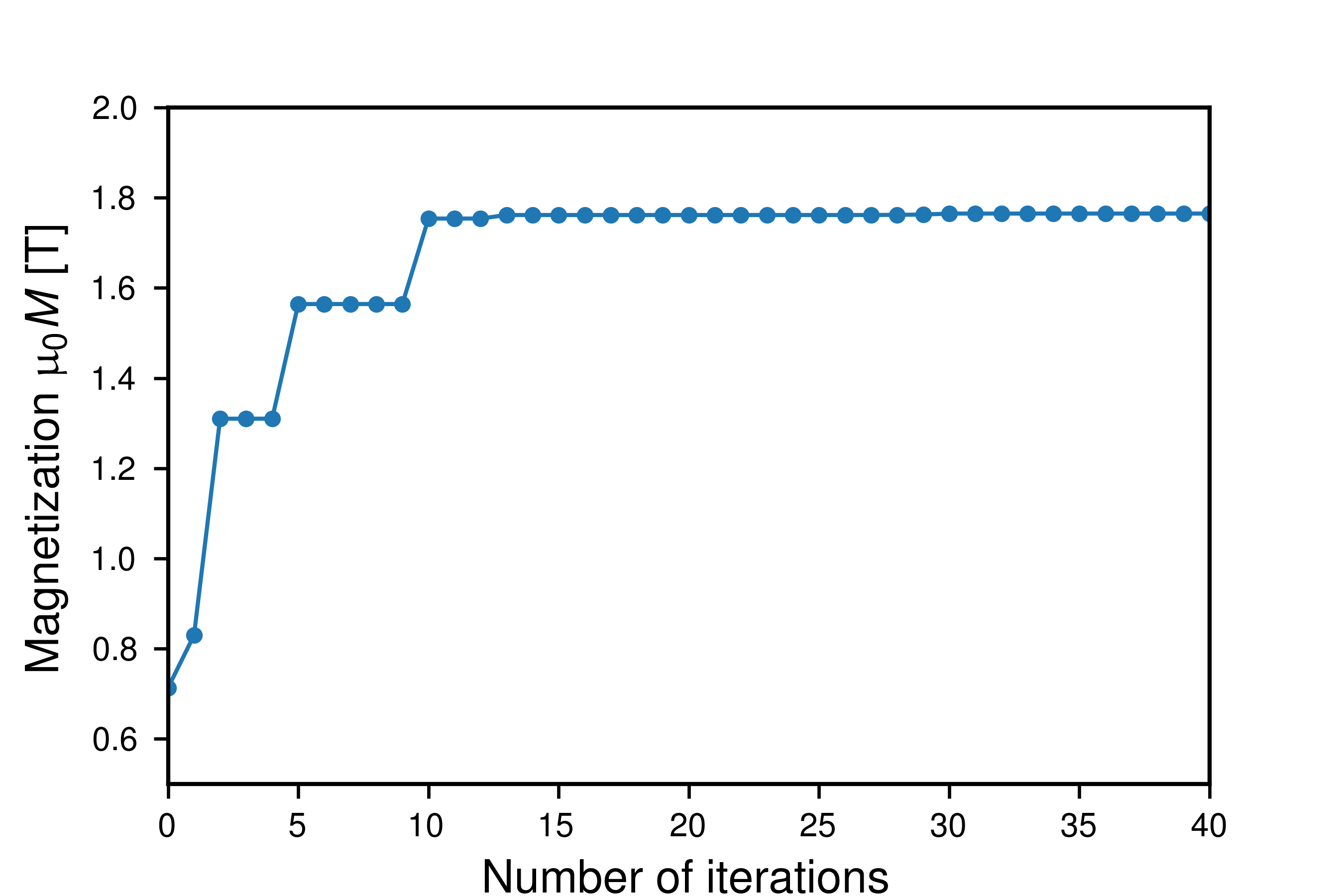
Figure 8: The best magnetization found in the loop of a session as a function of the number of iterations. The first result in a session corresponds to the point at the 0th iteration.

The highest magnetization found in the first $i$ iterations, $\max_{j\leq i}\,\mu_{0}M(j)$, is plotted against the number of iterations, $i$. In this run, the highest $\mu_{0}M$ in all the 3630 systems was found at 30th iteration where we define the zeroth iteration as that with the first sample. This process depends on a random sequence which is used in the sampling from the candidate lists. In order to take statistical profiles, we repeat the optimization scheme (which we call a session) 1,000 times.

To analyze the efficiency as a function of the number of iterations, we consider a cumulative distribution $\mathcal{D}_{i}(s)$ that is defined as the number of the sessions in which a system with a higher score than $s$ is found in the first $i$ iterations. We show a plot of $\mathcal{D}_{i}(s)$ in Bayesian optimization of magnetization using the descriptor #8 as the left figure in Fig. 9, where the horizontal axis shows the number of iterations, $i$, and the vertical axis shows the score variable, $s$. We also show a plot of the cumulative probability $\mathcal{P}_{i}(s)$ in the random sampling that is analytically obtained at the right-hand side. Because we took an enough number of sessions, there is negligible difference between the two figures for the first 10 iterations. The efficiency in the left figure suddenly becomes improved when the Bayesian optimization is switched on.

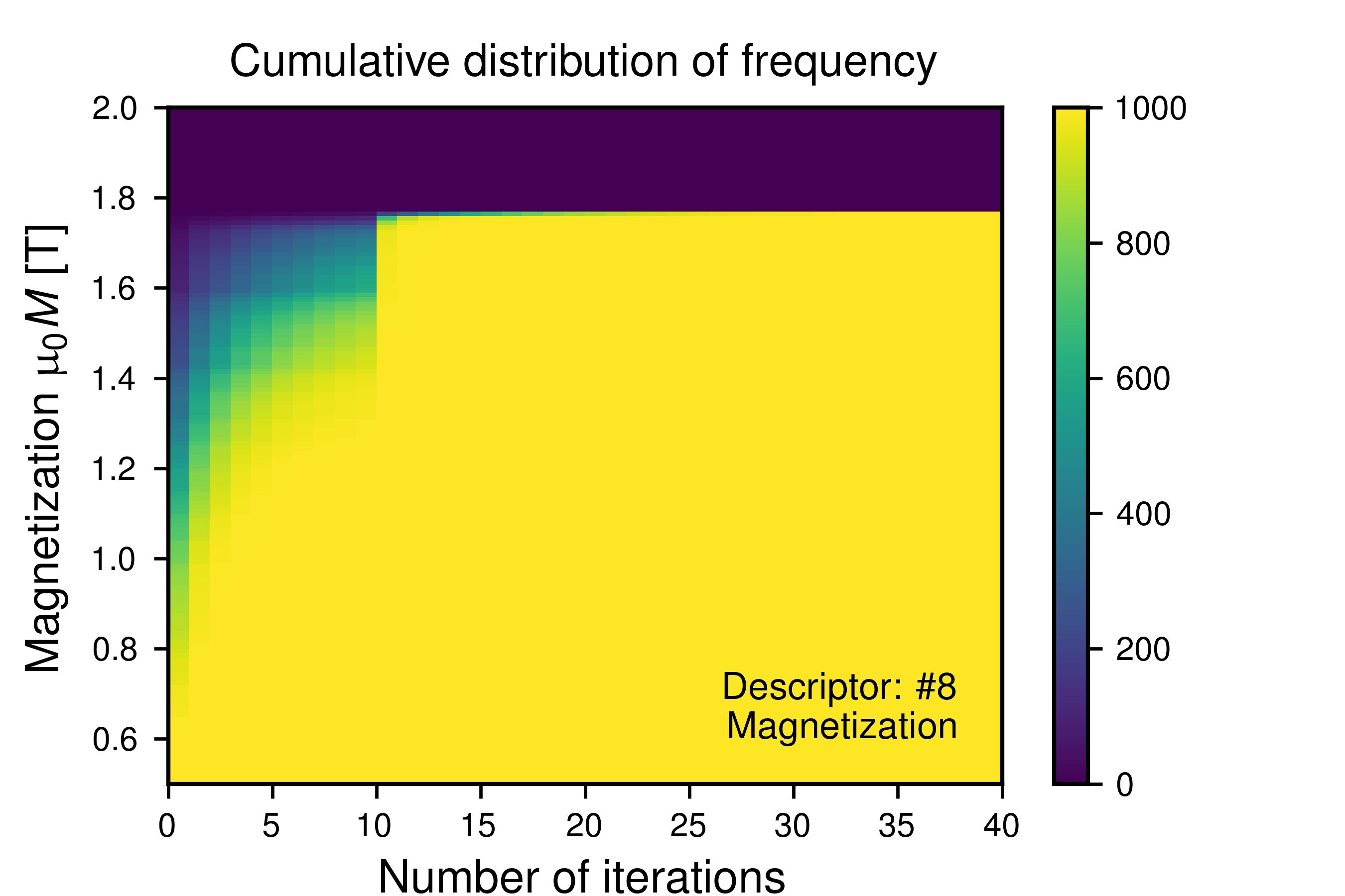
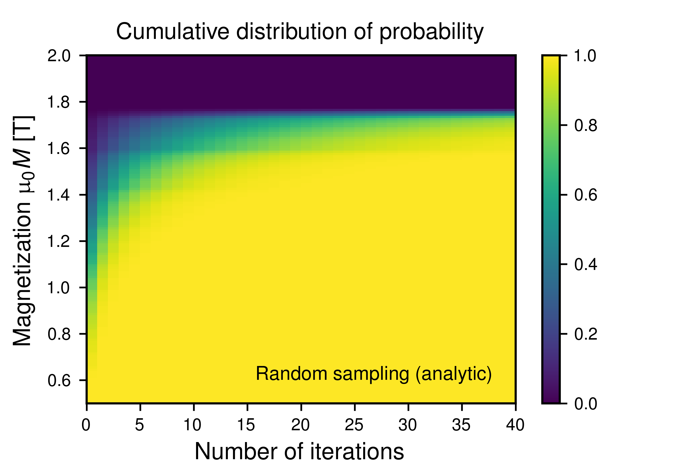
Figure 9: (Left) The cumulative distribution of frequency $\mathcal{D}_{i}(s)$ in the optimization of magnetization using the Bayesian optimization with the descriptor #8. (Right) The cumulative probability of probability $\mathcal{P}_{i}(s)$ that is analytically calculated for the optimization of magnetization with the random sampling.

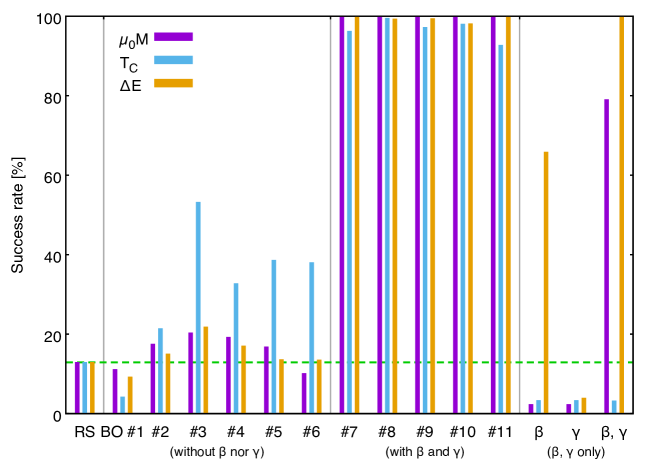
Figure 10: Success rate of finding the systems with the top 10 values of magnetization ($\mu_{0}M$), Curie temperature ($T_{\text{C}}$) and formation energy from the unary systems ($\Delta E$) among the 3630 candidates within 50 steps. RS stands for the random search; BO stands for the Bayesian optimization. The descriptors used in the search are shown along the horizontal axis: the numbers denote the descriptors listed in Table 1; the label $\beta$, $\gamma$ and $\beta,\gamma$ denote the results with using $\beta$, $\gamma$ and $\beta,\gamma$ as descriptors, respectively. The horizontal dashed line (green) is an eye-guide to show the height of the bars for the random sampling.

Figure 10 shows the success rate of finding the systems with the top 10 values of the target properties—magnetization ($\mu_{0}M$), Curie temperature ($T_{\text{C}}$) and formation energy from the unary systems ($\Delta E$)—within 50 steps. The results with Bayesian optimization (BO) are compared with the search by the random sampling (RS). The numbers with # in the figure denote the descriptors listed in Table 1. We find that the efficiency significantly depends on the choice of the descriptor. It is obvious from the figure that the descriptors #7–11 are very efficient in Bayesian optimization and much superior to those with #1–6 and the random sampling. This clearly shows that $\beta$ and $\gamma$ are important factors because the descriptors #7–11 differs from #2–6 only by $\beta$ and $\gamma$ used instead of $N_{\mathrm{T}}$.

This example demonstrates how we can incorporate domain knowledge into the machine learning. It is known that the magnetization of ferromagnetic random alloys of Fe and another transition metal is usually a well-behaved function of the number of the valence electrons. It is called Slater-Pauling curve. This curve can be reproduced well by first-principles calculation with CPADederichs et al. (1991), and so is the Slater-Pauling-like curve for the Curie temperature.Takahashi et al. (2007) These effects have also been observed in ThMn₁₂-type compounds experimentally,Buschow (1991); Hirayama et al. (2017) and explained theoretically.Miyake et al. (2014); Harashima et al. (2015b, 2016); Fukazawa et al. (2018); Harashima et al. (2018) On the basis of these previous researches, we were able to expect that including $\beta$ [the Co/(Fe+Co) ratio] and $\gamma$ (the Ti content) into the descriptor would improve the efficiency of the search in advance.

However, we also find that $\beta$ and $\gamma$ alone do not work as an efficient descriptor. The results of the Bayesian optimization with using $\beta$, $\gamma$, and the pair of them as descriptors are also shown in Fig. 10. Those success rates are significantly lower than the rates with the descriptors #7–11. This is because there are 66[= 3 (for R) $\times$ 2 (for Z) $\times$ 11 (for $\alpha$)] candidates that has common values of $\beta$ and $\gamma$ on the list, and 50 steps are not enough to obtain an adequate Bayesian model and draw one of the top 10 systems by chance. It is noteworthy that the efficiency of the Bayesian optimization is largely improved by adding only $N_{\mathrm{2a}}$ as in the descriptor #7.

Figure 11 shows the 95% (950 sessions) contour of $D_{i}(s)$ obtained with the descriptors #1–11. The best 95% of the data points are laid above those curves.

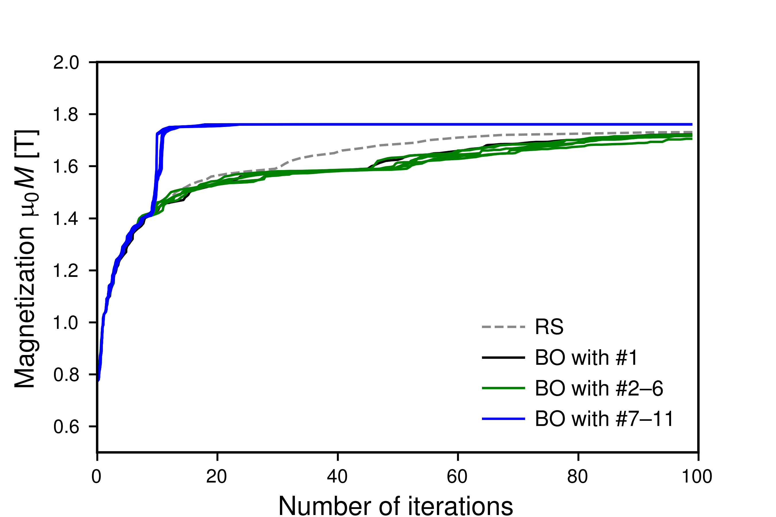
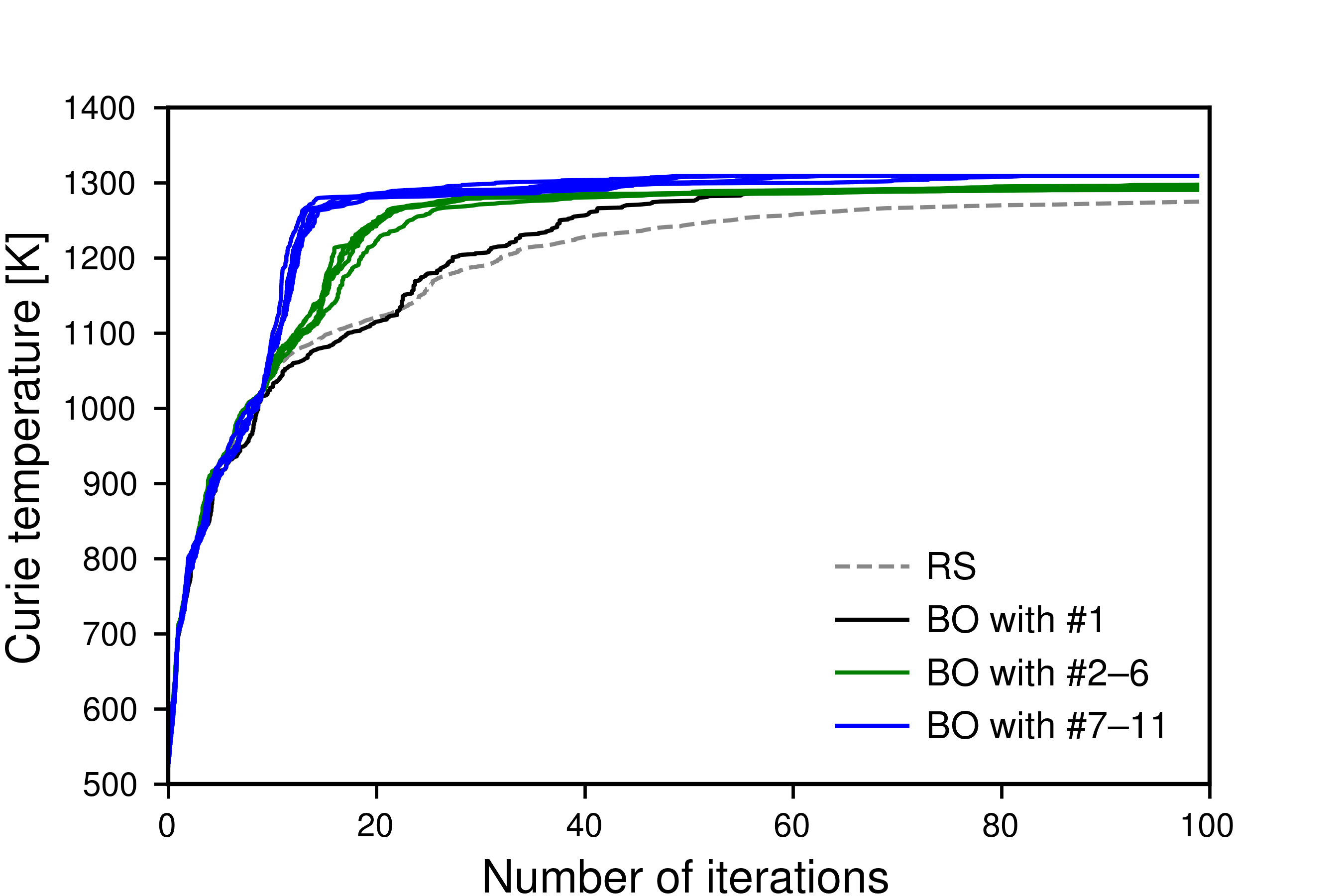
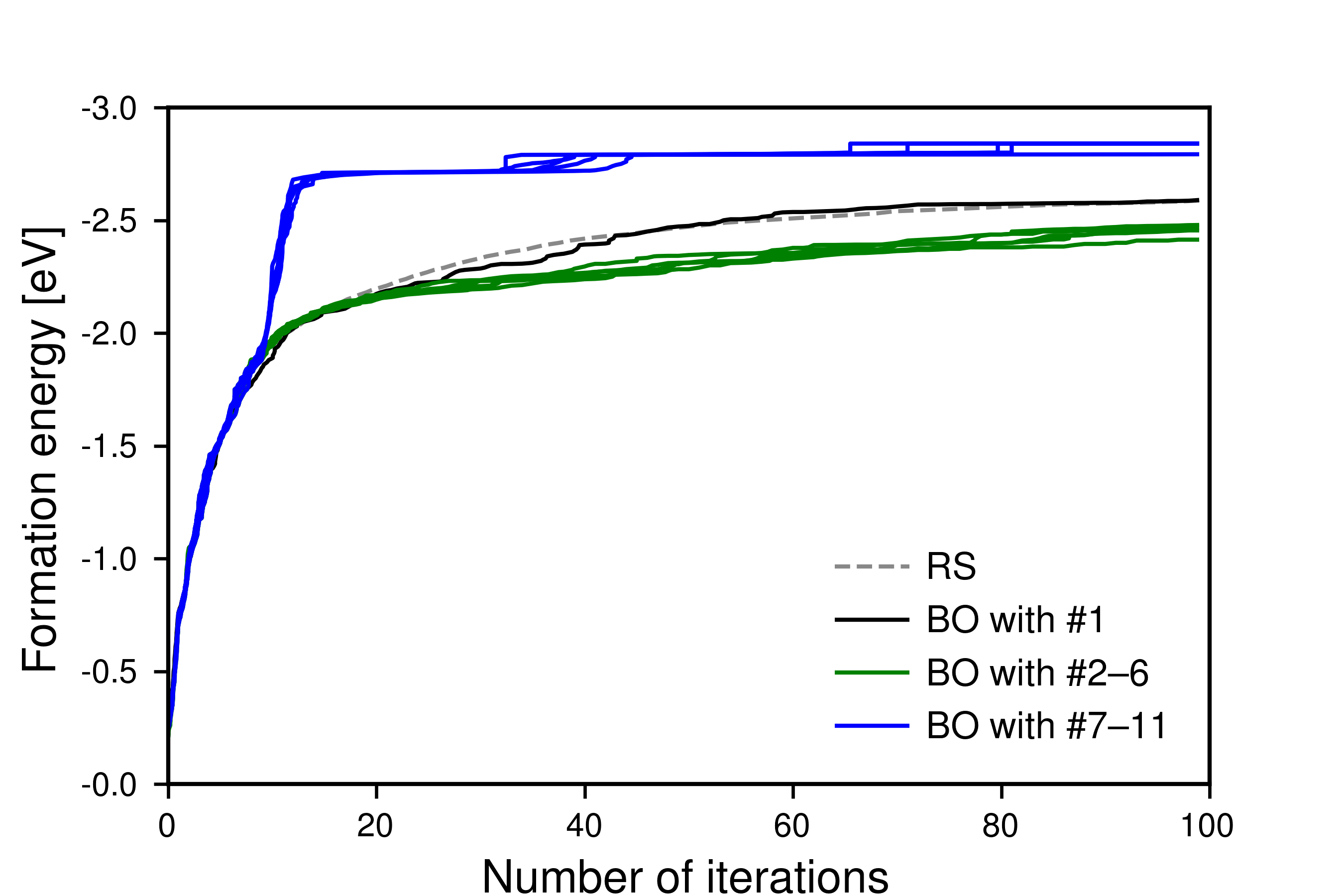
Figure 11: The 95% contours of the cumulative distribution $D_{i}(s)$ in the random sampling (gray dashed) and in the Bayesian optimizations with the descriptor #1 (black), the descriptors #2–6 (green) and the descriptors #7–11 (blue). The horizontal axis shows $i$; the vertical axis shows $s$. The top, middle and bottom figures show results in the optimization of the magnetization, the Curie temperature within the mean-field approximation, and the formation energy from the unary systems, respectively.

The panels show results with the random search and the Bayesian optimization with the descriptors #1–11. As shown in these graphs, the efficiency of the search depends much on the target property to optimize. The descriptors #7–11, which are with $\beta$ and $\gamma$, has a satisfying efficiency, with which even 20 iterations are enough to obtain a nearly best score regardless of the target property. The situation is quite different with the descriptors #1–6. In the optimization of the Curie temperature, these descriptors works efficiently. However, the optimizations of the magnetization and the formation energy progress even more slowly than the random sampling.

This difference between the Curie temperature and the other targets is also seen in Fig. 12, where the pair of $\beta$ and $\gamma$ is used as descriptors. The pair descriptor works as efficient as the descriptors #7–11 in the optimization of the magnetization and the formation energy. However, discernible difference in efficiency exists in the optimization of the Curie temperature. This suggests importance of information about elements at the 2a site (R and Z), which is consistent with Dam et al’s observation that the concentration of rare-earth elements is important in explaining the Curie temperature of binary alloys composed of a rare-earth element and a 3d transition-metal.Dam et al. (2018)

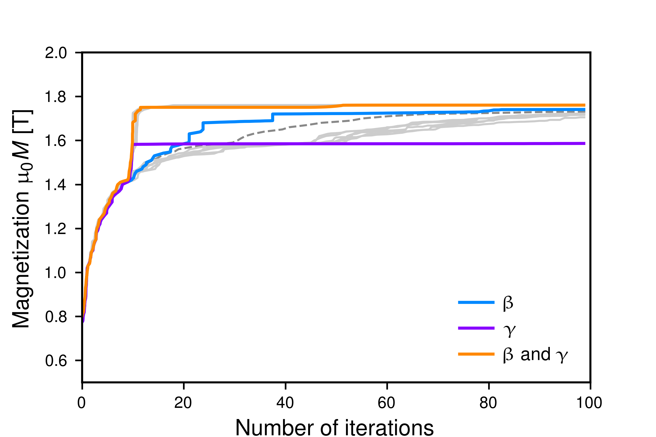
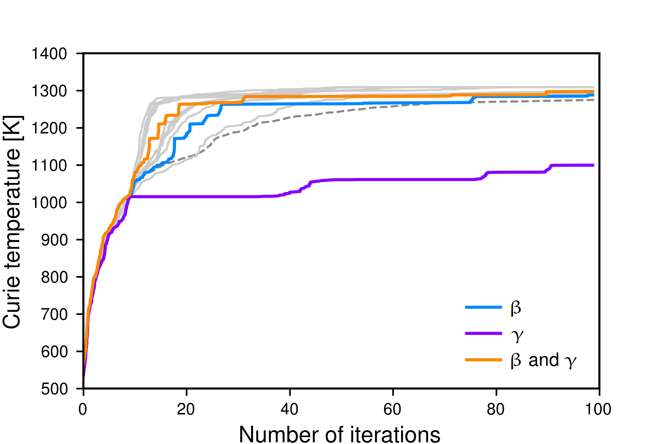
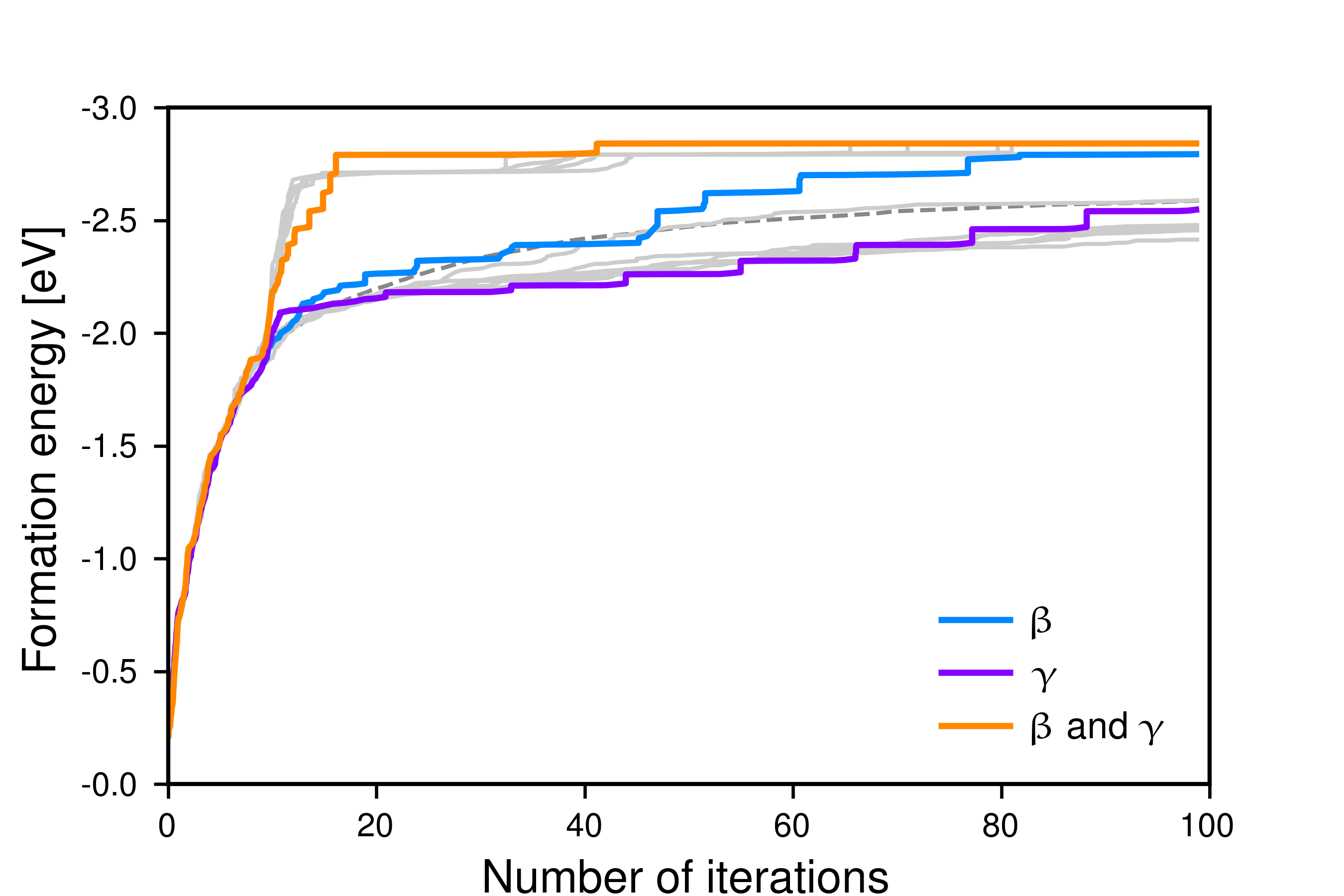
Figure 12: The 95% contours of the cumulative distribution $D_{i}(s)$ in the Bayesian optimizations with the descriptor $\beta$ (cyan), the descriptor $\gamma$ (purple) and the descriptor $(\beta,\gamma)$ (orange). Those in the random sampling and in the Bayesian optimization with the other descriptors are also shown as gray lines. The horizontal axis shows $i$; the vertical axis shows $s$. The top, middle and bottom figures show results in the optimization of the magnetization, the Curie temperature within the mean-field approximation, and the formation energy from the unary systems, respectively.

Dependency of the search efficiency on the the dimension of the descriptor is also noteworthy. When the dimension of a descriptor is large, the descriptor can accommodate a large search space on the one hand. However, modeling tends to be difficult with a higher dimensional space, which is referred as “curse of dimensionality”, on the other hand. Note that we have descriptors with 4 different dimensions in the groups of the descriptors #1–6 and #7–11. Figure 11 shows that the dimension has only a minor effect on the efficiency. This dependence is magnified by the more stringent criterion of the top-10 benchmark as shown in Fig. 10, especially in the results with the descriptor #1–6. However, the difference among the descriptor #7–11 are still subtle. Therefore, we expect that it would be safe to include six or a little more variables into the descriptor when we optimize for another target property.

V Conclusion

In this paper, we presented a machine-learning scheme for searching high-performance magnetic compounds. Our scheme is based on Bayesian optimization, and has a much higher efficiency than random sampling. We demonstrated its efficiency by taking the example of optimization of magnetization, Curie temperature and formation energy for the search space of magnet compounds having the ThMn₁₂ structure. One of the typical results is the success rate of finding the top 10 systems with the highest properties when 50 systems are sampled from a candidate list of 3630 systems (Fig. 10). The success rate is more than 90% with our scheme when the descriptor is appropriately chosen while it is approximately 10% in the random sampling.

The efficiency is maximized when we include the Co content ($\beta$), the Ti content ($\gamma$), and the information of the R and Z elements (e.g. $N_{\mathrm{2a}}$) into the descriptor. This improvement is what we could expect from the previous studies of magnet compounds. We stressed that it is important to incorporate domain knowledge into the choice of a descriptor. We also discussed how many variables a descriptor can accommodate without deteriorating the search efficiency. Although an excessive addition of variables to the descriptor can lose the efficiency of the search, there was not a significant loss when we doubled the dimension of the optimal descriptor.

We also proposed an integration scheme of two datasets to improve accuracy of an inexpensive large-sized dataset with using an accurate and small-sized dataset (reference dataset). The algorithm (Alg. 1 and 2) is easy to implement and fast. Prediction with a confidence bound (or the standard deviation $\tilde{S}$) is another feature of the scheme. We have also shown how it worked in the calculation of the formation energy (Fig. 7).

Appendix A Lattice parameters

Table 2 lists the lattice parameters for RCo₁₂ we used in the calculations. We assumed the ThMn₁₂ structure [space group: I4/mmm (#139)] for the system. The definitions of $p_{\text{8i}}$ and $p_{\text{8j}}$ are summarized in Table 3 with representable atomic positions of the atoms.

Table 2: Optimized lattice parameters for RCo₁₂ (R = Y, Nd, Sm). See Table 3 for definitions of $p_{\rm 8i}$ and $p_{\rm 8j}$.

R	$a$ [Å]	$c$ [Å]	$p_{\rm 8i}$	$p_{\rm 8j}$
Y	8.282	4.659	0.3585	0.2738
Nd	8.336	4.677	0.3590	0.2695
Sm	8.309	4.669	0.3587	0.2715

Table 3: Representable atomic positions in the ThMn₁₂ structure. The variables, $x$, $y$, and $z$, denote the point ($ax$, $ay$, $cz$) in Cartesian coordinates.

Element	Site	$x$	$y$	$z$
Th	2a	0	0	0
Mn	8f	0.25	0.25	0.25
Mn	8i	$p_{\rm 8i}$	0	0
Mn	8j	$p_{\rm 8j}$	0.5	0

In our KKR-CPA calculations for RFe₁₁Ti (R=Y, Nd, Sm) and ZFe₁₁Ti (Z=Zr, Dy), we assumed that they also have the ThMn₁₂ structure. The lattice parameters are reduced from the structure obtained in Ref. Harashima et al., 2015a and the structure given in Table 4. The value of $\sqrt{ab}$ is used as the $a$ parameter for the reduced cell to keep the cell volume. The inner parameters are determined so that the they minimize the deviation in the space of the coefficients $(x,y,z)$ of the unit vectors, which corresponds to the point ($ax$,$by$,$cz$) in the Cartesian coordinates. The reduced values are listed in Table 5.

Table 4: Inner coordinates $(x,y,z)$ of Fe and Ti in DyFe₁₁Ti and ZrFe₁₁Ti where Dy and Zr are placed at (0, 0, 0). The position of Ti is denoted by a parenthesis. These values corresponds to the point ($ax$, $by$, $cz$) in Cartesian coordinates where $a=8.455$, $b=8.262$ and $c=4.715$ in ZrFe₁₁Ti, and $a=8.518$, $b=8.410$ and $c=4.727$ in DyFe₁₁Ti.

	Fe(8f)			Fe(8i)			Fe(8j)
	$x$	$y$	$z$	$x$	$y$	$z$	$x$	$y$	$z$
DyFe11Ti	$0.255$	$0.251$	$0.251$	($0.375$	$0.000$	$0.000$)	$0.272$	$0.500$	$0.000$
	$0.255$	$0.749$	$0.749$	$-0.348$	$0.000$	$0.000$	$-0.266$	$0.500$	$0.000$
	$0.755$	$0.249$	$0.751$	$0.005$	$0.355$	$0.000$	$0.506$	$0.286$	$0.000$
	$0.755$	$0.751$	$0.249$	$0.005$	$-0.355$	$0.000$	$0.506$	$-0.286$	$0.000$
ZrFe11Ti	$0.256$	$0.250$	$0.251$	($0.381$	$0.000$	$0.000$)	$0.276$	$0.500$	$0.000$
	$0.256$	$0.750$	$0.750$	$-0.342$	$0.000$	$0.000$	$-0.264$	$0.500$	$0.000$
	$0.756$	$0.250$	$0.751$	$0.007$	$0.352$	$0.000$	$0.507$	$0.300$	$0.000$
	$0.756$	$0.750$	$0.250$	$0.007$	$-0.352$	$0.000$	$0.507$	$-0.300$	$0.000$

Table 5: Reduced values of the lattice parameters for RFe₁₁Ti (R = Y, Nd, Sm) and ZFe₁₁Ti (R = Zr, Dy). See Table 3 for definitions of $p_{\rm 8i}$ and $p_{\rm 8j}$.

Z	$a$ [Å]	$c$ [Å]	$p_{\rm 8i}$	$p_{\rm 8j}$
Y	8.476	4.730	0.3606	0.2764
Nd	8.560	4.701	0.3596	0.2703
Sm	8.523	4.713	0.3590	0.2728
Zr	8.358	4.715	0.3565	0.2850
Dy	8.464	4.727	0.3584	0.2776

Appendix B Integration model with a linear term

In this section, we incorporate an adjustable linear term into the relation of $E[\vec{x}]$ and $E^{\prime}[\vec{x}]$, which appear in Section III.3: we consider $E^{\prime}[\vec{x}]$ as an approximate function of $E[\vec{x}]+\vec{a}\cdot\vec{x}+b$ in this section.

This changes Eq. (3) to

$$\tilde{E}_{i}[\vec{y}]-E[\vec{x}^{\text{\,R}}_{i}]=E^{\prime}[\vec{y}]-E^{\prime}[\vec{x}^{\text{\,R}}_{i}]+\vec{a}\cdot\left(\vec{y}-\vec{x}^{\text{\,R}}_{i}\right)+\varepsilon_{i}.$$ (13)

Therefore, our model does not depend on the variable $b$.

Equation (7) is modified as follows:

$$\tilde{\mu}=E^{\prime}[\vec{y}]+\frac{1}{\Omega}\sum_{i}\omega_{i}\left\{E[\vec{x}^{\text{\,R}}_{i}]-E^{\prime}[\vec{x}^{\text{\,R}}_{i}]+\vec{a}\cdot\left(\vec{y}-\vec{x}^{\text{\,R}}_{i}\right)\right\},$$ (14)

while Eq. (8) is left unchanged.

The estimation by the maximum likelihood method with $\tilde{E}_{\text{LOO},i}$ described in Section III.3 is applicable to the variable $\vec{a}$ and $\sigma^{2}$. The equation for $\vec{a}$ is

$$\left(\sum_{i}\frac{1}{\Omega_{\text{LOO},i}}\vec{\xi}_{i}\otimes\vec{\xi}_{i}\right)\vec{a}=\sum_{i}\left(E[\vec{x}^{\text{\,R}}_{i}]-E^{\prime}[\vec{x}^{\text{\,R}}_{i}]-\frac{1}{\Omega_{\text{LOO},i}}\sum_{k\neq i}\omega_{k}\left\{E[\vec{x}^{\text{\,R}}_{k}]-E^{\prime}[\vec{x}^{\text{\,R}}_{k}]\right\}\right)$$ (15)

where $\vec{\xi}_{i}$ is defined as

$$\vec{\xi}_{i}\equiv\sum_{k\neq i}\omega_{k}\{\vec{x}^{\text{\,R}}_{i}-\vec{x}^{\text{\,R}}_{k}\}$$ (16)

and the symbol $\otimes$ denotes the dyadic product, with which $(\alpha_{1},\alpha_{2},\alpha_{3})\otimes(\beta_{1},\beta_{2},\beta_{3})$ is defined as the matrix whose $(i,j)$ component is $\alpha_{i}\beta_{j}$. This equation can be solved for $\vec{a}$ without determining $\sigma^{2}$.

The equation for $\sigma^{2}$ is modified as

$$\sigma^{2}=\frac{1}{M}\sum_{i}\Omega_{\text{LOO},i}\left(E[\vec{x}^{\text{\,R}}_{i}]-E^{\prime}[\vec{x}^{\text{\,R}}_{i}]-\frac{\sum_{k\neq i}\omega_{k}\left\{E[\vec{x}^{\text{\,R}}_{k}]-E^{\prime}[\vec{x}^{\text{\,R}}_{k}]+\vec{a}\cdot\left(\vec{x}^{\text{\,R}}_{i}-\vec{x}^{\text{\,R}}_{k}\right)\right\}}{\Omega_{\text{LOO},i}}\right)^{2}.$$

Appendix C Dimensions for R and Z

We prepared dimensions to include information of the R and Z elements in our design of the descriptors in Table 1. Because the corresponding choice is only 6 in combination (R = Y, Nd, Sm; Z = Zr, Du) while it is known that high-dimensionality often causes problems in modeling, readers may doubt its necessity. We compare the efficiency of search for the smaller space in which those elements are fixed to R = Y and Z = Zr in Fig. 13. The solid line along the cross symbols in the figures denote the frequency of finding the system with the best score out of 1000 sessions in the restricted space when we use the set of $\alpha,\beta$ and $\gamma$ as a descriptor. We also show the curve elongated 6 times along $x$-axis (the dotted line) because one has to optimize also for the other combinations of R and Z to obtain the optimal system for the full space, which approximately takes 6 times larger. For comparison, we show the result of optimization for the full space using the descriptor #9 by the line along the circle points. We set the number of iterations before Bayesian optimization to 5, which is smaller than the number we use above (=10), because we know that the full-space search is so fast that the search in the smaller space cannot catch up if it starts 60 (=$10\times 6$) iterations behind (Fig. 10 and 11). We see from Fig.13 that the search with the full space is more efficient, even with this setup, than repeating the search for the small space 6 times. Therefore, the dimensions for R and Z actually contribute to the search efficiency.

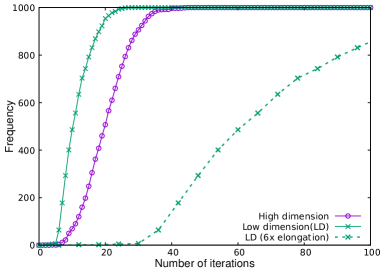
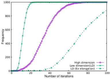
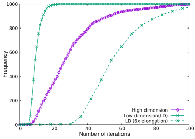
Figure 13: Frequency of finding the system with the highest magnetization (top), Curie temperature (middle), and the lowest formation energy (bottom) among 1000 sessions. Those in the search for the small space where R and Z are fixed to R = Y and Z = Zr are denoted by the solid line along cross symbols. The dotted line along cross symbols show the curve elongated 6 times along $x$-axis. The line along the circle symbols show the result of the search in the full space using the descriptor #9 in Table 1.

Appendix D Data from the first-principles calculations

In this section, we list systems with the predicted highest values of magnetization and Curie temperature in order to make a comparison with available experimental data and to serve a guiding information for future experimental synthesis.

In Table 6, we show the top 10 systems of the highest magnetization. Here we add the contribution of the f-electrons of Nd, Sm and Dy with the assumption that those have $g_{J}J$ of 3.27, 0.71 and $-10$ $\mu_{B}$. Due to this additional magnetic moment, the systems with Nd has advantage over the other systems, and all the top 10 systems have Nd in them.

It should also be noted that the values for the formation energy are positive for all the top 10 systems, and violate a necessary condition for the thermodynamic stability. The highest magnetization among the systems with a negative value of the formation energy is obtained by Nd(Fe_0.7Co_0.3)₁₂. Note also that this does not ensure the stability against the other phases. We also show the values for (Sm_0.7Zr_0.3)(Fe_0.9Co_0.1)₁₂ because the magnetic anisotropy of Nd tend not to be uniaxial in ThMn₁₂-type systems in the absence of a third element.

The best system, NdFe₁₂, has already been synthesized by Hirayama et al.Hirayama et al. (2015a) From the results of our calculations, this system seems to be near the upper limit of the magnetization at absolute zero.

Table 6: The top 10 systems with the highest values of the magnetization. The magnetic moment from the f-electrons is assumed to be 3.27 $\mu_{\mathrm{B}}$ for Nd, 0.71 $\mu_{\mathrm{B}}$ for Sm, $-10$ $\mu_{\mathrm{B}}$ for Dy. The variable $\mu_{0}M$ denotes the magnetization, $T_{\mathrm{C}}$ the Curie temperature, and $\Delta E$ the formation energy from the unary systems. The values for Nd(Fe_0.7Co_0.3)₁₂, which has the highest magnetization among the systems with a negative formation energy, and the values for (Sm_0.7Zr_0.3)(Fe_0.9Co_0.1)₁₂, which has the highest magnetization among the systems having Sm in them with a negative formation energy, are also shown.

Formula	$\mu_{0}M$ [T]	$T_{\mathrm{C}}$ [K]	$\Delta E$ [eV]
NdFe12	1.95	844	0.405
Nd(Fe0.9Co0.1)12	1.94	1012	0.230
Nd(Fe0.8Co0.2)12	1.93	1111	0.095
(Nd0.9Zr0.1)Fe12	1.93	835	0.443
(Nd0.9Zr0.1)(Fe0.9Co0.1)12	1.92	1011	0.272
(Nd0.9Zr0.1)(Fe0.8Co0.2)12	1.91	1098	0.140
(Nd0.8Zr0.2)Fe12	1.91	841	0.446
(Nd0.8Zr0.2)(Fe0.9Co0.1)12	1.91	1009	0.272
(Nd0.7Zr0.3)Fe12	1.89	845	0.385
(Nd0.8Zr0.2)(Fe0.8Co0.2)12	1.89	1086	0.143
Nd(Fe0.7Co0.3)12	1.89	1143	-0.142
(Sm0.7Zr0.3)(Fe0.9Co0.1)12	1.77	1002	-0.008

In Table 7, we show the top 10 systems with the highest values of Curie temperature. Although the formation energy is negative for all the systems in the table, it should be noted again that those incorporate only the competition with the unary phases and does not ensure the stability against the other phases.

The best system in the list is Sm(Fe_0.2Co_0.8)₁₂. Although Hirayama et al. have reported that they could synthesize Sm(Fe_0.8Co_0.2)₁₂ as a film, there is no experimental report for a successful synthesis of compounds with higher concentration of Co to our knowledge.

Table 7: The top 10 systems with the highest values of the Curie temperature. The variable $\mu_{0}M$ denotes the magnetization, $T_{\mathrm{C}}$ the Curie temperature, and $\Delta E$ the formation energy from the unary systems.

Formula	$T_{\mathrm{C}}$ [K]	$\mu_{0}M$ [T]	$\Delta E$ [eV]
Sm(Fe0.2Co0.8)12	1310	1.47	-0.631
(Sm0.9Dy0.1)(Fe0.2Co0.8)12	1309	1.39	-0.654
(Sm0.8Dy0.2)(Fe0.2Co0.8)12	1307	1.32	-0.676
(Sm0.7Dy0.3)(Fe0.2Co0.8)12	1305	1.24	-0.696
(Sm0.6Dy0.4)(Fe0.2Co0.8)12	1304	1.17	-0.715
(Sm0.5Dy0.5)(Fe0.2Co0.8)12	1302	1.09	-0.733
(Sm0.4Dy0.6)(Fe0.2Co0.8)12	1300	1.01	-0.752
(Nd0.7Dy0.3)(Fe0.2Co0.8)12	1300	1.37	-0.553
(Nd0.6Dy0.4)(Fe0.2Co0.8)12	1299	1.27	-0.594
(Nd0.8Dy0.2)(Fe0.2Co0.8)12	1299	1.46	-0.510

References

- Rupp et al. (2012) Matthias Rupp, Alexandre Tkatchenko, Klaus-Robert Müller, and O Anatole Von Lilienfeld, “Fast and accurate modeling of molecular atomization energies with machine learning,” Physical review letters 108, 058301 (2012).
- Ghiringhelli et al. (2015) Luca M Ghiringhelli, Jan Vybiral, Sergey V Levchenko, Claudia Draxl, and Matthias Scheffler, “Big data of materials science: critical role of the descriptor,” Physical review letters 114, 105503 (2015).
- Seko et al. (2015) Atsuto Seko, Atsushi Togo, Hiroyuki Hayashi, Koji Tsuda, Laurent Chaput, and Isao Tanaka, “Prediction of low-thermal-conductivity compounds with first-principles anharmonic lattice-dynamics calculations and bayesian optimization,” Physical review letters 115, 205901 (2015).
- Pham et al. (2016) Tien Lam Pham, Hiori Kino, Kiyoyuki Terakura, Takashi Miyake, and Hieu Chi Dam, “Novel mixture model for the representation of potential energy surfaces,” The Journal of Chemical Physics 145, 154103 (2016).
- Lam Pham et al. (2017) Tien Lam Pham, Hiori Kino, Kiyoyuki Terakura, Takashi Miyake, Koji Tsuda, Ichigaku Takigawa, and Hieu Chi Dam, “Machine learning reveals orbital interaction in materials,” Science and technology of advanced materials 18, 756–765 (2017).
- Dam et al. (2018) Hieu Chi Dam, Viet Cuong Nguyen, Tien Lam Pham, Anh Tuan Nguyen, Kiyoyuki Terakura, Takashi Miyake, and Hiori Kino, “Important descriptors and descriptor groups of Curie temperatures of rare-earth transition-metal binary alloys,” Journal of the Physical Society of Japan 87, 113801 (2018).
- Pham et al. (2018) Tien-Lam Pham, Nguyen-Duong Nguyen, Van-Doan Nguyen, Hiori Kino, Takashi Miyake, and Hieu-Chi Dam, “Learning structure-property relationship in crystalline materials: A study of lanthanide–transition metal alloys,” The Journal of chemical physics 148, 204106 (2018).
- Ouyang et al. (2018) Runhai Ouyang, Stefano Curtarolo, Emre Ahmetcik, Matthias Scheffler, and Luca M Ghiringhelli, “SISSO: A compressed-sensing method for identifying the best low-dimensional descriptor in an immensity of offered candidates,” Physical Review Materials 2, 083802 (2018).
- Seko et al. (2018) Atsuto Seko, Hiroyuki Hayashi, Hisashi Kashima, and Isao Tanaka, “Matrix-and tensor-based recommender systems for the discovery of currently unknown inorganic compounds,” Physical Review Materials 2, 013805 (2018).
- Ueno et al. (2016) Tsuyoshi Ueno, Trevor David Rhone, Zhufeng Hou, Teruyasu Mizoguchi, and Koji Tsuda, “COMBO: An efficient Bayesian optimization library for materials science,” Materials discovery 4, 18–21 (2016).
- Ju et al. (2017) Shenghong Ju, Takuma Shiga, Lei Feng, Zhufeng Hou, Koji Tsuda, and Junichiro Shiomi, “Designing nanostructures for phonon transport via bayesian optimization,” Physical Review X 7, 021024 (2017).
- Kikuchi et al. (2018) Shun Kikuchi, Hiromi Oda, Shin Kiyohara, and Teruyasu Mizoguchi, “Bayesian optimization for efficient determination of metal oxide grain boundary structures,” Physica B: Condensed Matter 532, 24–28 (2018).
- Yuan et al. (2018) Ruihao Yuan, Zhen Liu, Prasanna V Balachandran, Deqing Xue, Yumei Zhou, Xiangdong Ding, Jun Sun, Dezhen Xue, and Turab Lookman, “Accelerated discovery of large electrostrains in BaTiO3-based piezoelectrics using active learning,” Advanced Materials 30, 1702884 (2018).
- Oganov and Valle (2009) Artem R Oganov and Mario Valle, “How to quantify energy landscapes of solids,” The Journal of chemical physics 130, 104504 (2009).
- Kennedy and O’Hagan (2000) Marc C Kennedy and Anthony O’Hagan, “Predicting the output from a complex computer code when fast approximations are available,” Biometrika 87, 1–13 (2000).
- Pilania et al. (2017) Ghanshyam Pilania, James E Gubernatis, and Turab Lookman, “Multi-fidelity machine learning models for accurate bandgap predictions of solids,” Computational Materials Science 129, 156–163 (2017).
- Pan et al. (2010) Sinno Jialin Pan, Qiang Yang, et al., “A survey on transfer learning,” IEEE Transactions on knowledge and data engineering 22, 1345–1359 (2010).
- Hutchinson et al. (2017) Maxwell L Hutchinson, Antono Erin, Brenna M Gibbons, Sean Paradiso, Julia Ling, and Bryce Meredig, “Overcoming data scarcity with transfer learning,” (2017).
- Ohashi et al. (1988a) Ken Ohashi, Yoshio Tawara, Ryo Osugi, Junji Sakurai, and Yukitomo Komura, “Identification of the intermetallic compound consisting of sm, ti, fe,” J. Less-Common Met. 139, L1–L5 (1988a).
- Ohashi et al. (1988b) K. Ohashi, Y. Tawara, R. Osugi, and M. Shimao, “Magnetic properties of fe‐rich rare‐earth intermetallic compounds with a thmn12 structure,” J. Appl. Phys. 64, 5714–5716 (1988b).
- Yang et al. (1988) Ying-chang Yang, Lin-shu Kong, Shu-he Sun, Dong-mei Gu, and Ben-pei Cheng, “Intrinsic magnetic properties of SmTiFe10,” Journal of applied physics 63, 3702–3703 (1988).
- Verhoef et al. (1988) R Verhoef, FR De Boer, Zhang Zhi-dong, and KHJ Buschow, “Moment reduction in RFe12-xTx compounds (R = Gd, Y and T= Ti, Cr, V, Mo, W),” Journal of Magnetism and Magnetic Materials 75, 319–322 (1988).
- De Mooij and Buschow (1988) DB De Mooij and KHJ Buschow, “Some novel ternary ThMn12-type compounds,” Journal of the Less Common Metals 136, 207–215 (1988).
- Buschow (1988) K. H. J. Buschow, “Structure and properties of some novel ternary Fe‐rich rare‐earth intermetallics (invited),” J. Appl. Phys. 63, 3130–3135 (1988).
- Jaswal et al. (1990) S. S. Jaswal, Y. G. Ren, and D. J. Sellmyer, “Electronic structure and magnetic properties of Fe‐rich ternary compounds: YFe10V2 and YFe10Cr2,” J. Appl. Phys. 67, 4564–4566 (1990).
- Coehoorn (1990) R. Coehoorn, “Electronic structure and magnetism of transition-metal-stabilized intermetallic compounds,” Phys. Rev. B 41, 11790–11797 (1990).
- Buschow (1991) K H J Buschow, “Permanent magnet materials based on tetragonal rare earth compounds of the type RFe12-xMx,” Journal of magnetism and magnetic materials 100, 79–89 (1991).
- Sakurada et al. (1992) S. Sakurada, A. Tsutai, and M. Sahashi, “A study on the formation of ThMn12 and NaZn13 structures in RFe10Si2,” Journal of Alloys and Compounds 187, 67–71 (1992).
- Sakuma (1992) Akimasa Sakuma, “Self-Consistent Band Calculations for YFe11Ti and YFe11TiN,” J. Phys. Soc. Jpn. 61, 4119–4124 (1992).
- Asano et al. (1993) S. Asano, S. Ishida, and S. Fujii, “Electronic structures and improvement of magnetic properties of RFe12X (R = Y, Ce, Gd; X = N, C),” Physica B 190, 155 – 168 (1993).
- Akayama et al. (1994) M. Akayama, H. Fujii, K. Yamamoto, and K. Tatami, “Physical properties of nitrogenated RFe11Ti intermetallic compounds (R=Ce, Pr and Nd) with ThMn12-type structure,” J. Magn. Magn. Mater. 130, 99 – 107 (1994).
- Kuz’min et al. (1999) M. D. Kuz’min, M. Richter, and K. H. J. Buschow, “Iron-rich versus cobalt-rich ThMn12-type intermetallics: a comparative study of the crystal fields,” Solid State Commun. 113, 47 – 51 (1999).
- Gabay et al. (2016) A. M. Gabay, A. Martín-Cid, J. M. Barandiaran, D. Salazar, and G. C. Hadjipanayis, “Low-cost Ce1-xSmx(Fe, Co, Ti)12 alloys for permanent magnets,” AIP Advances 6, 056015 (2016), https://doi.org/10.1063/1.4944066 .
- Körner et al. (2016) Wolfgang Körner, Georg Krugel, and Christian Elsässer, “Theoretical screening of intermetallic thmn12-type phases for new hard-magnetic compounds with low rare earth content,” Scientific Reports 6, 24686 (2016).
- Ke and Johnson (2016) Liqin Ke and Duane D. Johnson, “Intrinsic magnetic properties in (Fe1-xCox)11Ti (Y and Ce; = H, C, and N),” Phys. Rev. B 94, 024423 (2016).
- Fukazawa et al. (2017) Taro Fukazawa, Hisazumi Akai, Yosuke Harashima, and Takashi Miyake, “First-principles study of intersite magnetic couplings in NdFe12 and NdFe12X (X= B, C, N, O, F),” Journal of Applied Physics 122, 053901 (2017).
- Fukazawa et al. (2019) Taro Fukazawa, Hisazumi Akai, Yosuke Harashima, and Takashi Miyake, “First-principles study of spin-wave dispersion in Sm(Fe1-xCox)12,” Journal of Magnetism and Magnetic Materials 469, 296 – 301 (2019).
- Miyake et al. (2014) Takashi Miyake, Kiyoyuki Terakura, Yosuke Harashima, Hiori Kino, and Shoji Ishibashi, “First-Principles Study of Magnetocrystalline Anisotropy and Magnetization in NdFe12, NdFe11Ti, and NdFe11TiN,” Journal of the Physical Society of Japan 83, 043702 (2014).
- Hirayama et al. (2015a) Y Hirayama, YK Takahashi, S Hirosawa, and K Hono, “NdFe12Nx hard-magnetic compound with high magnetization and anisotropy field,” Scripta Materialia 95, 70–72 (2015a).
- Hirayama et al. (2015b) Yusuke Hirayama, Takashi Miyake, and Kazuhiro Hono, “Rare-earth lean hard magnet compound NdFe12N,” JOM 67, 1344–1349 (2015b).
- Yang et al. (1991a) Ying-chang Yang, Xiao-dong Zhang, Lin-shu Kong, Qi Pan, and Sen-lin Ge, “New potential hard magnetic material—NdTiFe11Nx,” Solid state communications 78, 317–320 (1991a).
- Yang et al. (1991b) Ying-chang Yang, Xiao-dong Zhang, Sen-lin Ge, Qi Pan, Lin-shu Kong, Hailin Li, Ji-lian Yang, Bai-sheng Zhang, Yong-fan Ding, and Chun-tang Ye, “Magnetic and crystallographic properties of novel fe-rich rare-earth nitrides of the type RTiFe11N1-δ,” Journal of applied physics 70, 6001–6005 (1991b).
- Harashima et al. (2016) Yosuke Harashima, Kiyoyuki Terakura, Hiori Kino, Shoji Ishibashi, and Takashi Miyake, “First-principles study on stability and magnetism of NdFe and NdFeN for M= Ti, V, Cr, Mn, Fe, Co, Ni, Cu, Zn,” Journal of Applied Physics 120, 203904 (2016).
- Hirayama et al. (2017) Y Hirayama, Y K Takahashi, S Hirosawa, and K Hono, “Intrinsic hard magnetic properties of Sm(Fe1-xCox)12 compound with the ThMn12 structure,” Scripta Materialia 138, 62–65 (2017).
- Suzuki et al. (2014) S. Suzuki, T. Kuno, K. Urushibata, K. Kobayashi, N. Sakuma, K. Washio, H. Kishimoto, A. Kato, and A. Manabe, “A (Nd, Zr)(Fe, Co)11.5Ti0.5Nx compound as a permanent magnet material,” AIP Adv. 4, 117131 (2014).
- Sakuma et al. (2016) N. Sakuma, S. Suzuki, T. Kuno, K. Urushibata, K. Kobayashi, M. Yano, A. Kato, and A. Manabe, “Influence of Zr substitution on the stabilization of ThMn12-type (Nd1-αZrα)(Fe0.75Co0.25)11.25Ti0.75N (),” AIP Adv. 6, 056023 (2016).
- Kuno et al. (2016) Tomoko Kuno, Shunji Suzuki, Kimiko Urushibata, Kurima Kobayashi, Noritsugu Sakuma, Masao Yano, Akira Kato, and Akira Manabe, “(Sm,Zr)(Fe,Co)Ti compounds as new permanent magnet materials,” AIP Adv. 6, 025221 (2016).
- Suzuki et al. (2016) S. Suzuki, T. Kuno, K. Urushibata, K. Kobayashi, N. Sakuma, K. Washio, M. Yano, A. Kato, and A. Manabe, “A new magnet material with ThMn12 structure: (Nd1-xZrx)(Fe1-yCoy)11+zTi1-zNα(),” J. Magn. Magn. Mater. 401, 259–268 (2016).
- Harashima et al. (2018) Yosuke Harashima, Taro Fukazawa, Hiori Kino, and Takashi Miyake, “Effect of -site substitution and pressure on stability of Fe12: A first-principles study,” arXiv preprint arXiv:1805.12241 (2018).
- (50) “COMmon Bayesian Optimization Library (COMBO),” https://github.com/tsudalab/combo.
- Hohenberg and Kohn (1964) Pierre Hohenberg and Walter Kohn, “Inhomogeneous electron gas,” Physical Review 136, B864 (1964).
- Kohn and Sham (1965) Walter Kohn and Lu Jeu Sham, “Self-consistent equations including exchange and correlation effects,” Physical Review 140, A1133 (1965).
- Jensen and Mackintosh (1991) Jens Jensen and Allan R Mackintosh, Rare earth magnetism (Clarendon Oxford, 1991).
- Richter (1998) Manuel Richter, “Band structure theory of magnetism in 3d-4f compounds,” Journal of Physics D: Applied Physics 31, 1017 (1998).
- Locht et al. (2016) I. L. M. Locht, Y. O. Kvashnin, D. C. M. Rodrigues, M. Pereiro, A. Bergman, L. Bergqvist, A. I. Lichtenstein, M. I. Katsnelson, A. Delin, A. B. Klautau, B. Johansson, I. Di Marco, and O. Eriksson, “Standard model of the rare earths analyzed from the hubbard i approximation,” Phys. Rev. B 94, 085137 (2016).
- Perdew and Zunger (1981) J. P. Perdew and Alex Zunger, “Self-interaction correction to density-functional approximations for many-electron systems,” Phys. Rev. B 23, 5048–5079 (1981).
- Blöchl (1994) P. E. Blöchl, “Projector augmented-wave method,” Phys. Rev. B 50, 17953–17979 (1994).
- Kresse and Joubert (1999) G. Kresse and D. Joubert, “From ultrasoft pseudopotentials to the projector augmented-wave method,” Phys. Rev. B 59, 1758–1775 (1999).
- (59) “QMAS—Quantum MAterials Simulator Official Site,” http://qmas.jp.
- Perdew et al. (1996) John P. Perdew, Kieron Burke, and Matthias Ernzerhof, “Generalized gradient approximation made simple,” Phys. Rev. Lett. 77, 3865–3868 (1996).
- Fukazawa et al. (2018) Taro Fukazawa, Hisazumi Akai, Yosuke Harashima, and Takashi Miyake, “First-principles study of intersite magnetic couplings and Curie temperature in RFe12-xCrx (R = Y, Nd, Sm),” Journal of Physical Society of Japan 87, 044706 (2018).
- Harashima et al. (2015a) Yosuke Harashima, Kiyoyuki Terakura, Hiori Kino, Shoji Ishibashi, and Takashi Miyake, “First-principles study of structural and magnetic properties of R(Fe,Ti)12 and R(Fe,Ti)12N (R= Nd, Sm, Y),” in Proceedings of Computational Science Workshop 2014 (CSW2014), JPS Conference Proceedings, Vol. 5 (2015) p. 1021.
- Soven (1967) Paul Soven, “Coherent-potential model of substitutional disordered alloys,” Physical Review 156, 809 (1967).
- Soven (1970) Paul Soven, “Application of the coherent potential approximation to a system of muffin-tin potentials,” Physical Review B 2, 4715 (1970).
- Shiba (1971) Hiroyuki Shiba, “A reformulation of the coherent potential approximation and its applications,” Progress of Theoretical Physics 46, 77–94 (1971).
- Liechtenstein et al. (1987) A I Liechtenstein, M I Katsnelson, V P Antropov, and V A Gubanov, “Local spin density functional approach to the theory of exchange interactions in ferromagnetic metals and alloys,” Journal of Magnetism and Magnetic Materials 67, 65–74 (1987).
- Fukazawa et al. (in press) Taro Fukazawa, Hisazumi Akai, Yosuke Harashima, and Takashi Miyake, “Curie temperature of Sm2Fe17 and Nd2Fe14B: a first-principles study,” IEEE Transaction on Magnetics (in press).
- Dederichs et al. (1991) P H Dederichs, R Zeller, H Akai, and H Ebert, “Ab-initio calculations of the electronic structure of impurities and alloys of ferromagnetic transition metals,” Journal of magnetism and magnetic materials 100, 241–260 (1991).
- Takahashi et al. (2007) C Takahashi, M Ogura, and H Akai, “First-principles calculation of the Curie temperature Slater–Pauling curve,” Journal of Physics: Condensed Matter 19, 365233 (2007).
- Harashima et al. (2015b) Yosuke Harashima, Kiyoyuki Terakura, Hiori Kino, Shoji Ishibashi, and Takashi Miyake, “Nitrogen as the best interstitial dopant among =B, C, N, O, and F for strong permanent magnet : First-principles study,” Phys. Rev. B 92, 184426 (2015b).