On the varied origins of up-bending breaks in galaxy disks

Abstract

Aims. Using a sample of 175 low-inclination galaxies from the S⁴G, we investigate the origins of up-bending (Type III) breaks in the 3.6 $\mu$m surface brightness profiles of disk galaxies.

Methods. We re-analyze a sample of previously identified Type III disk break-hosting galaxies using a new, unbiased break-finding algorithm, which uncovered many new, sometimes subtle disk breaks across the whole sample. We classify each break by its likely origin through close examination of the galaxy images across wavelengths, and compare samples of galaxies separated by their outermost identified break types in terms of their stellar populations and local environments.

Results. We find that more than half of the confirmed Type III breaks in our sample can be attributed to morphological asymmetry in the host galaxies. As these breaks are mostly an artifact of the azimuthal averaging process, their status as physical “breaks” is questionable. Such galaxies occupy some of the highest density environments in our sample, implying that much of this asymmetry is the result of tidal disturbance. Additionally, we find that Type III breaks related to extended spiral arms or star formation often host down-bending (Type II) breaks at larger radius which were previously unidentified. Such galaxies reside in the lowest density environments in our sample, in line with previous studies that found a lack of Type II breaks in clusters. Galaxies occupying the highest density environments most often show Type III breaks associated with outer spheroidal components.

Conclusions. We find that Type III breaks in the outer disks of galaxies arise most often through environmental influence: either tidal disturbance (resulting in disk asymmetry) or heating through, e.g., galaxy harrassment (leading to spheroidal components). Galaxies hosting the latter break types also show bimodal distributions in central $g-r$ color and morphological type, with more than half of such galaxies classified as Sa or earlier; this suggests these galaxies may be evolving into early-type galaxies. By contrast, we find that Type III breaks related to apparently secular features (e.g., spiral arms) may not truly define their hosts’ outer disks, as often in such galaxies additional significant breaks can be found at larger radius. Given this variety in Type III break origins, we recommend in future break studies making a more detailed distinction between break subtypes when seeking out, for example, correlations between disk breaks and environment, to avoid mixing unlike physical phenomena.

1 Introduction

The outer regions of disk galaxies are important tracers of galaxy formation and evolution. Their radial extent and coherent rotation make them particularly sensitive to environmental influences, the effects of which are preserved over long periods by extended dynamical timescales. Outer disks also serve as excellent laboratories for the evolution of galaxies at low mass surface density, probing the connection between disk stability and star formation (e.g., Kennicutt 1989; Martin & Kennicutt 2001; Thilker et al. 2007; Goddard et al. 2010) and the preponderance of stellar migration across disks through interactions with bars, spiral arms, or satellites (e.g., Sellwood & Binney 2002; Debattista et al. 2006; Roškar et al. 2008; Minchev et al. 2012; Ruiz-Lara et al. 2017). This low mass surface density also yields highly inefficient star formation (Bigiel et al. 2010), despite gas dominating the mass budget (e.g. Broeils & Rhee 1997; Sancisi et al. 2008), a situation reflective of many dwarf galaxies (e.g., van Zee et al. 1997; Bigiel et al. 2010; Elmegreen & Hunter 2015).

Stellar disks often show abrupt truncations or anti-truncations in their radial surface brightness profiles at extended radii (e.g., Freeman 1970; van der Kruit 1987; Pohlen & Trujillo 2006; Erwin et al. 2008; Gutiérrez et al. 2011; Martín-Navarro et al. 2012; Laine et al. 2014), giving clues to how mass is distributed across the disk throughout the galaxy’s lifetime. Since the seminal work by Pohlen & Trujillo (2006) and Erwin et al. (2008), disk galaxies have been separated into three major classes (following and expanding upon the system devised by Freeman 1970): Type I disks, with surface brightness profiles described well by a single exponential decline; Type II disks, best described by a broken exponential with a steeper decline in the disk outskirts; and Type III disks, described by a broken exponential with a shallower decline in the outskirts. Type II disk breaks, the most common (Pohlen & Trujillo 2006; Erwin et al. 2008; Laine et al. 2014), are also perhaps the most well-understood; often their presence is attributed to a combination of a dynamical star formation threshold (e.g., Kennicutt 1989; Martin & Kennicutt 2001), which truncates the young stellar disk, and radial migration, which populates the disk beyond the break radius with evolved stars (e.g., Sellwood & Binney 2002; Debattista et al. 2006; Bakos et al. 2008; Roškar et al. 2008; Minchev et al. 2011; Muñoz-Mateos et al. 2013).

The most poorly understood breaks are those of Type III, for which a wide variety of explanations have been proffered. Younger et al. (2007), for example, showed that Type III breaks can arise through accretion of a gas-rich companion, while Laurikainen & Salo (2001) found that shallow outer profiles are often introduced into Messier 51-like interacting pairs through long-lived redistributions of mass. Kinematic heating of stellar populations through major mergers (Borlaff et al. 2014), bombardment by cold dark matter substructure (Kazantzidis et al. 2009), and galaxy harassment (Roediger et al. 2012) may form some Type III disk breaks as well. Tidally induced isophotal asymmetry may also often lead to Type III disk breaks (Erwin et al. 2005; Laine et al. 2014), and because S0 galaxies host such breaks more frequently than late-type spirals, regardless of environment (e.g. Erwin et al. 2005; Gutiérrez et al. 2011; Ilyina & Sil’chenko 2012; Maltby et al. 2015), Type III disk break formation and S0 formation may be linked. In some cases (denoted Type IIIh or IIIs; Pohlen & Trujillo 2006; Erwin et al. 2008), Type III breaks may instead reflect a transition to a kinematically hot stellar component, such as the stellar halo (Martín-Navarro et al. 2012, 2014; Peters et al. 2017) or thick disk (Comerón et al. 2012, 2018).

In the realm of star formation, Laine et al. (2016; hereafter, L16) found that disk scalelengths beyond Type III breaks in their sample were longest in the u-band, suggesting predominantly young trans-break populations. Similarly, Wang et al. (2018) showed that Type III disks are more prevalent in low-spin, HI-rich galaxies, suggesting that star formation induced through gas accretion results in Type III breaks. Enhanced star formation in the inner disk may also yield steeper inner disk profiles than outer disk profiles, thereby producing anti-truncations (Hunter & Elmegreen 2006). Some Type III breaks have been linked to outer rings or pseudorings (Erwin et al. 2005; Pohlen & Trujillo 2006), and in simulations have been linked to scattering by bars (Herpich et al. 2017), implying that internal secular processes can also lead to Type III breaks. In this vein, Type III breaks may also arise through a combination of accretion events and outward radial migration (e.g., Ruiz-Lara et al. 2017), or migration induced by infall into a cluster environment (e.g., Clarke et al. 2017).

It is worth summarizing these possibilities: Type III breaks may result from minor mergers, major mergers, flyby interactions, dark matter substructure, harassment, stellar halos, thick disks, enhanced outer disk star formation, enhanced inner disk star formation, outer rings, bar scattering, radial migration, and other internal secular processes in both isolated and interacting galaxies. These explanations span nearly every possible aspect of disk galaxy evolution.

Comparitive studies of disk breaks, by necessity, do not take this diversity into account, assessing only the relative frequencies or average properties of Type I, Type II, and Type III disk break hosts (e.g., Pohlen & Trujillo 2006; Bakos et al. 2008; Gutiérrez et al. 2011; Roediger et al. 2012; Laine et al. 2014; Maltby et al. 2015; Wang et al. 2018). If each type of break can be created through such a diverse array of mechanisms, however, this approach may lack the complexity necessary for a complete understanding of disk breaks. Indeed, this diversity may be one reason different disk break studies come to conflicting conclusions: for example, one might expect that if most Type III disk breaks resulted from enhanced outer disk star formation (L16, Wang et al. 2018), evidence of this would appear through frequent blueward color gradients in Type III disks. Yet Bakos et al. (2008) and Zheng et al. (2015) found that, on average, Type III color profiles are flat. Also, if many Type III disk breaks form through tidal disturbance (e.g., Erwin et al. 2005; Laine et al. 2014), their hosts should be more often found in dense environments. Yet several studies of late-type galaxies either failed to find such a correlation (e.g., Pohlen & Trujillo 2006; Maltby et al. 2012), or found only a weak such correlation (e.g., Laine et al. 2014).

Therefore, to elucidate the formation mechanisms of Type III disk breaks, we perform a detailed re-analysis of the 3.6 $\mu$m images of Type III break-hosting galaxies in the Spitzer Survey of Stellar Structure in Galaxies (S⁴G; Sheth et al. 2010), as previously classified by L16. We introduce a new unbiased break-finding algorithm and incorporate the detailed morphological classifications of Buta et al. (2015) into both the break identification and interpretation. We then classify each identified break using a new system of break subclassifications tailored to the apparent physical origin of each break, and explore the stellar populations of the break hosts and correlations between the break subcategories and the local environment. In Section 2, we discuss the datasets used in this study, as well as the chosen sample of galaxies. In Section 3, we discuss our break-finding methodology, and present an overview of our break classification scheme. Section 4 presents the results of our study, including color profiles by break type and environmental correlation with break type. Section 5 provides a discussion of the potential physical origins and data-driven causes of these break subcategories, and Section 6 provides a summary.

2 Sample and Data

To facilitate comparisons with previous work, we selected our sample from that defined by L16, an expansion of the sample defined by Laine et al. (2014) to include later Hubble types and lower stellar masses. In summary, the sample was chosen from the the S⁴G (Sheth et al. 2010) and the Near InfraRed S0-Sa Survey (NIRS0S; Laurikainen et al. 2011), including only those galaxies with Hubble types $-2\leq T\leq 9$ (using the near-IR classifications from Laurikainen et al. 2011; Buta et al. 2015) and minor/major axis ratios $b/a>0.5$ (as measured from the outer disk). This sample covers Local Universe galaxies with a wide range of stellar masses ($8\lesssim\log_{10}(M_{*}/M_{\odot})\lesssim 11$, albeit with systematically lower masses for Hubble types T$\gtrsim 5$; see Fig. 1 of L16), and through the axis ratio restriction includes only those galaxies for which the features in the surface brightness profiles can be tied to morphological features in the disks.

For the present study, we re-examined the 175 (of 753 total) galaxies L16 classified as having Type III breaks in one or more of the following bands: 3.6$\mu$m from the S⁴G survey; K_s-band from the NIRS0S survey; u, g, r, i, and z-band imaging from a re-reduction of Sloan Digital Sky Survey (SDSS, specifically DR7 & DR8; Abazajian et al. 2009; Aihara et al. 2011) images done by Knapen et al. (2014); and g-band imaging from the Liverpool Telescope for 111 S⁴G galaxies not found in SDSS (Knapen et al. 2014). The Type III sub-sample contains no NIRS0S survey galaxies, as many NIRS0S galaxies were removed from the original sample of Laine et al. (2014) by L16 through a combination of a tighter restriction on image depth and a revised T-type selection (T$\geq$-2, compared to T$\geq$-3). Additionally, we included any ambiguous Type III break classifications as well, for the sake of completeness and a larger sample size. For example, 5 galaxies in the present sample were classified as Type III disks only in optical bands, and 39 were given hybrid classifications (e.g., Type III+II). Color information from SDSS imaging is available for only 113 galaxies in our sample.

As L16, we use galaxy centers, position angles, axial ratios, background sky levels, and background standard deviations from Salo et al. (2015). We utilize the near-IR morphological classifications from Buta et al. (2015), as well as the foreground star, background galaxy, and artifact masks from Muñoz-Mateos et al. (2015), enlarged through dilation with a 3 pixel radius top-hat kernel in order to avoid spurious breaks at low surface brightness (see the Appendix).

While we used only the 3.6 $\mu$m images in our break-finding analysis, we measured surface brightness profiles in optical bands as well to derive radial color profiles. In all bands, we measured surface brightness profiles using elliptical apertures with fixed centers, position angles, and axial ratios derived from the 3.6 $\mu$m images using the IRAF ellipse package (Jedrzejewski 1987), with orientations and axial ratios reflective of each galaxy’s outer disk. Specifically, we measured the mean flux within each annular aperture $i$, $\bar{f}_{i}$ (with fixed widths of 1.5″, interpolating across masked regions), and derived the surface brightness as

$$\mu_{i}=-2.5\log_{10}(\bar{f}_{i})+\textrm{ZP}+2.5\log_{10}(p^{2})$$ (1)

where ZP is the surface brightness zero-point for the given band and $p$ is the pixel scale in arcsec px^-1.

We describe our break-finding algorithm using these one-dimensional profiles in the following section. We also provide a detailed assessment of methodological biases on the derivation of the surface brightness profiles in the Appendix, including the effects of masking, interpolation of flux across masks, and the use of the mean flux vs. the median flux in each aperture.

3 Break identification and classification

3.1 Break-finding algorithm

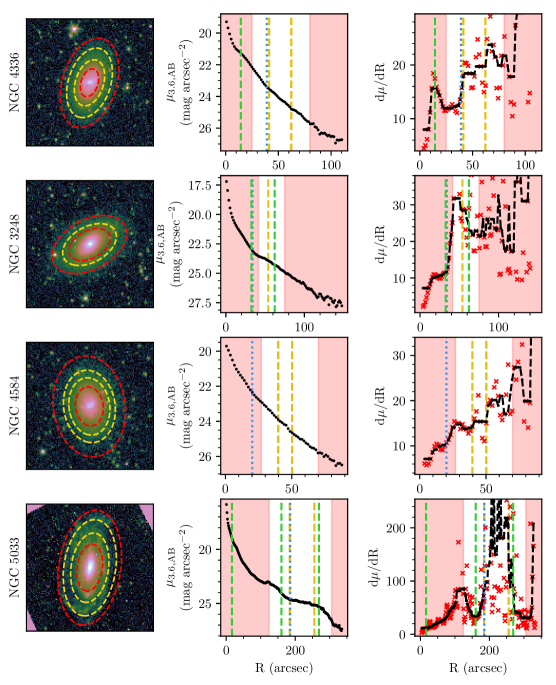
Figure 1: Demonstration of inner radius choice. The left column shows 3.6$\mu$m images of the demonstration galaxies, with the inner and outer radius fitting boundaries shown as red dashed ellipses and break radii as yellow ellipses. The middle column shows these galaxies’ 3.6$\mu$m surface brightness profiles. Red shaded regions denote the radial regions excluded from our break-finding procedure. Green dashed lines show the radii of inner rings, lenses, etc. used in determining the inner radius boundaries (see text), as well as outer rings, lenses etc. used for aiding in break classification. Yellow dashed lines mark break radii from our analysis, while blue dotted lines mark break radii from L16 (break classifications are discussed in more detail below). Finally, the right column shows the local slope of the surface brightness profile vs. radius; vertical lines are the same as in the middle column, and the red points show the local slope profile before median smoothing (see text). From the top row to the bottom, we demonstrate avoidance of: an inner ring; an inner lens; a non-exponential inner region; and an oval distortion.

To overcome some of the uncertainties in break classification, we have developed a new approach to identify breaks. First, we define inner radius boundaries by excluding from our analysis those regions satisfying the following criteria:

1. The region falls inside of the bar, inner ring, inner pseudoring, inner lens, or inner spiral arm radius, as measured by Herrera-Endoqui et al. (2015), if available (most inner spiral arm radii were not available, hence were estimated by eye).

2. The region is not well-characterized by an exponential profile.

These conditions avoid regions of the disk in which the shape of the surface brightness profile is evidently dominated by bars and related internal structures ($\theta$- or $\phi$-shaped regions, e.g.; Curtis 1918; Buta & Combes 1996), as well as non-exponential structures such as classical bulges. Bars are known to redistribute mass within spiral galaxies (e.g., Hohl 1971; Athanassoula & Misiriotis 2002; Debattista et al. 2006; Binney & Tremaine 2008; Minchev et al. 2011; Athanassoula 2013), thereby altering the surface brightness profile of the host (e.g., Pohlen & Trujillo 2006; Erwin et al. 2008; Muñoz-Mateos et al. 2013; Laine et al. 2014; Díaz-García et al. 2016a). We thus choose to focus on regions of the disk that are more likely to be influenced by external factors. We use the outer radius boundaries from L16, defined as the radius at which the surface brightness profile alters by $\pm$0.2 magnitudes with $\pm 1\sigma_{\rm sky}$ perturbations to the sky subtraction (as Pohlen & Trujillo 2006), where $\sigma_{\rm sky}$ is the standard deviation of the local background from Salo et al. (2015). We provide a few illustrative examples in Fig. 1 using four galaxies’ surface brightness and local slope profiles, plotted against radius.

Additionally, we excluded similar regions near oval distortions because of the way in which oval distortions act as bars (e.g., Kormendy & Norman 1979; Jogee et al. 2002; Kormendy & Kennicutt 2004; Trujillo et al. 2009). As a rough preliminary selection criterion, we identified oval galaxy candidates as those galaxies with inner isophotes showing deprojected axial ratios of $b/a\lesssim$0.8. This is a $\sim$4–5$\sigma$ deviation from circularity given the typical errors on the ellipticity (e.g., Muñoz-Mateos et al. 2015) in the outer isophotes from which the axial ratio and position angle used for deprojection were drawn. We then narrowed down this candidate list through visual inspection, e.g. seeking out outer spiral arms emerging from the ends of the oval, resulting in 23 oval disk candidates. However, in most cases this oval classification was ambiguous — for example, the change in axial ratio between the inner and outer isophotes was either very slight or very gradual — therefore in only 5 of 23 cases did we take this oval classification into consideration when defining our inner radius limits. For these 5 galaxies (e.g., NGC 5033, shown in Fig. 1), we chose to avoid the oval regions for both consistency (under the assumption they act as bars) and for simplicity, as the surface brightness profiles of such galaxies are extremely complex, showing upward of 5 significant changes in slope.

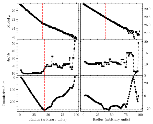
Figure 2: Demonstration of break-finding algorithm. Top: two idealized model Type III surface brightness profiles, with Poisson and simulated sky noise added. Both profiles use the same inner disk slope; the left profile contains a break with h${}_{\rm in}/$h${}_{\rm out}=0.5$, while the right profile contains a break with h${}_{\rm in}/$h${}_{\rm out}=0.9$. Red dashed lines mark the break radius. Middle: the local slope profiles of the model surface brightness profiles. The red dashed line in the left profile marks the break radius as determined by our break-finding algorithm. No significant break was found for the right profile. Bottom: the cumulative sums, as defined in Equation 2, with the break radius of the left profile again marked with a red dashed line. Gray dashed lines mark the locations of the maximum and minimum values of CS (in the text, max(CS) and min(CS)). Note that the minimum CS of the right profile occurs at the same location as the left profile; the break, however, was not found to be significant and is therefore not shown.

Once we defined the inner radius boundary, we measured the local slope of the surface brightness profile as a function of radius, following Pohlen & Trujillo (2006), i.e., using the four adjacent points on the curve at each radial bin, but smoothing the resulting slope profile with a median kernel with a width of 10% of the full extent of the array rather than 5%. We used four adjacent points to measure slope in order to balance the level of noise with resolution; a wider range tends to both shift the break location and wash out subtler breaks, for example. Likewise, we chose this kernel width to balance resolution with the often small angular size of the sample galaxies, the smallest of which contain only $\sim$30 radial bins (e.g., ESO 402-30). These choices influence only the subtlest breaks, and so have minimal impact on our conclusions.

To identify break radii, we used a statistical method called change-point analysis (Taylor 2000, reproduced in Python by the authors following the online technical description). In brief, this method searches for significant changes in the mean of a time-series (or similar profile) using the cumulative sum (hereafter, CS; Hinkley 1971). The CS is defined for a variable $x$ with sample size $N$ as:

$$CS_{0}=0,\textrm{ }CS_{N}=\sum_{j=1}^{N}(x_{j}-\bar{x})$$ (2)

where $\bar{x}$ is the mean of $x$. Hence, CS is actually the cumulative sum of the difference from the mean.

We show two examples of the break-finding method for idealized model Type III disks in Fig. 2, created as the sum of two exponentials (e.g., Erwin et al. 2008; Laine et al. 2014, with $\alpha$=2) with Poisson noise and artifical sky noise added to the flux at each radius. The left panels show a successful application of the technique on a fairly strong disk break (with the ratio of the inner to outer disk scale lengths h${}_{\rm in}/$h${}_{\rm out}=0.5$), while the right profile shows an example of a weak break buried in noise, where the algorithm fails (h${}_{\rm in}/$h${}_{\rm out}=0.9$, in this case). In the successful case in the left panels, because the innermost slope is consistently lower than the mean slope (roughly the average of the inner and outer slopes), the CS curve continually decreases until the change point; beyond the change point, the slope remains consistently higher than the mean, and the CS curve increases. The minimum of this profile therefore marks the break radius (the red dashed lines in Fig. 2). By counterexample, the CS curve of a Type II break galaxy would be inverted, and the change point would occur at the maximum.

We note that the agreement between the break location as defined by the algorithm with the true break location depends on the smoothness of the break. A least-squares fit (such as that done by Laine et al. 2014, L16) should provide more accurate break locations. That said, given that we find as many as three breaks in many galaxies in our re-analysis, the complexity of such profiles runs the risk of over-fitting the curves, therefore we choose simply to identify the points where the slope changes rather than fit a multi-parameter functional form. Because we are more concerned with the break classifications themselves than with the precise locations of the breaks, this choice does not alter any of the scientific conclusions in our paper.

We ran this break-finding algorithm three times per galaxy. The first locates the global minimum of the CS profile; we then split the profile at the identified break radius to locate additional significant changes in slope shortward and longward of the initial change point. Each galaxy thus was classified with a maximum of three disk breaks. This choice to split the profiles three times allowed us to identify locally important changes in slope in addition to global changes, thereby skirting the assumption that any given galaxy be primarily defined by just one disk break. In a few cases (NGC 4041, NGC5963, etc.) more than three significant disk breaks were identifiable through further splitting of the profile; for the sake of simplicity, however, we included only the three most significant breaks in the final classification.

To test the significance of each break, we employed a bootstrapping test following Hinkley & Schechtman (1987); Taylor (2000). For each galaxy, we recorded the first identified break’s strength (defined as $CS_{\rm diff}=$max$(CS)-$min$(CS)$). We then randomly reordered the galaxy’s radial slope profile, rederiving and recording the new location of the CS minimum and the new reordered break strength a total of $10^{5}$ times. If the break is significant, more often than not the break strength in the reordered profile will fall below that of the real profile. Therefore, we defined as significant those breaks for which $CS_{\rm diff}$ of the reordered CS profiles was less than $CS_{\rm diff}$ of the original profile in $\geq$95% of re-samplings. We then repeated this process for each additional break identified in the galaxy. We applied these significance tests to all breaks in all galaxies in the full sample. This process reduces the number of false positives caused by e.g. very minor or very localized changes of slope.

Next, to test the break resilience to the sky uncertainty, we perturbed the surface brightness profiles by adding and subtracting the 1$\sigma$ flux uncertainty in each radial bin $i$, defined as

$$\sigma_{i}^{2}=\sigma_{\rm sky}^{2}+\sigma_{\textrm{Poisson},i}^{2}$$ (3)

where $\sigma_{\rm sky}$ is the RMS in the background sky (using the values given by Salo et al. 2015, normalized by $\sqrt{N}$, with $N$ the number of pixels in each radial bin) and $\sigma_{\textrm{Poisson},i}$ is the Poisson uncertainty in the flux in bin $i$. We then repeat the break-finding analysis and bootstrap resampling procedure, rejecting all breaks if they fall below our 95% bootstrapping significance cutoff with either perturbation. This minimizes the inclusion of potentially spurious breaks resulting from improper background subtraction.

3.2 Break classification scheme

Our break-finding algorithm identified many new breaks across the galaxies in our sample compared to those previously identified by L16. Therefore, at the risk of adding complexity to an already complex subject, we adopt a new disk break classification scheme for our study, building from previous schemes (Pohlen & Trujillo 2006; Erwin et al. 2008; Laine et al. 2014). For reference, we provide a summary of the break types in Table 1. We also provide detailed justifications for all break classifications of all our sample galaxies, including: written justifications; radial profiles of surface brightness, local slope of surface brightness, projected and deprojected axial ratio and position angle, as well as $m=1$ and $m=2$ Fourier mode amplitude; and images, including 3.6$\mu$m, $g$-band (as well as unsharp-masked versions of each), deprojected 3.6$\mu$m images, and 3.6$\mu$m images masked to outline bright structures found in the disk. We used these profiles and images to aid in our break classifications, and make them available both through the Centre de Données astronomiques de Strasbourg (CDS) and at the following URL: https://www.oulu.fi/astronomy/S4G_TYPE3_DISC_BREAKS/breaks.html

Table 1: Break Classification Summary

Type 0:	Not exponential
Type I:	No significant disk break
Type IId:	Down-bending break at spirals, lenses, rings, etc.
Type IIa:	Down-bending break at asymmetric feature (e.g., tidal stream)
Type IIIa:	Up-bending break at asymmetric feature
Type IIId:	Up-bending break marking symmetric outer disklike features, e.g., spiral arms or HII regions
Type IIIs:	Up-bending break marking outer spheroidal component

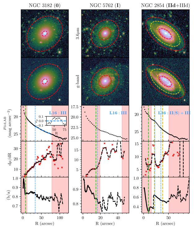
Figure 3: Examples of our break classification scheme. We show here galaxies of Type 0 (left), Type I (middle), and a Type IId break (right, innermost break). These are reclassifications of galaxies with Type III breaks identified by L16. Bold text indicates the break being demonstrated, and the original break classifications are provided in the third row panels. Ellipses are as in Fig. 1. The third row shows the 3.6$\mu$m surface brightness profile (AB magnitudes) vs. radius. The inset in the left panel shows the residuals to a linear fit (shown as the dashed blue line) to the surface brightness profile beyond the break radius, demonstrating its non-exponential nature. The fourth row shows the local slope of the surface brightness profile vs. radius. The fifth row shows the galaxy’s on sky axial ratio vs. radius. Vertical lines and shaded regions are as in Fig. 1. See the text for specific details on each galaxy’s break classification.

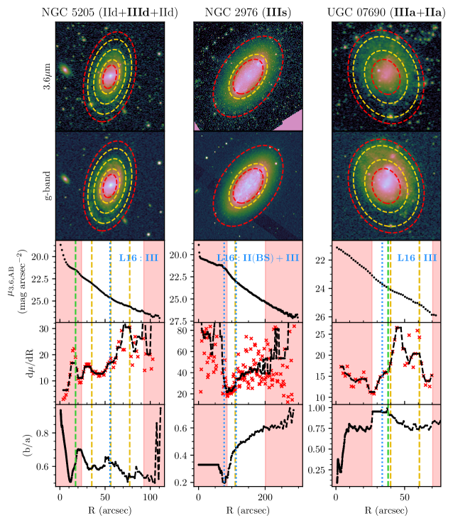
Figure 4: As Fig. 3, now demonstrating a Type IIId break (left column), a Type IIIs break (middle column), and Type IIIa and IIa breaks (right column), each again reclassifications of Type III break hosts as identified by L16. Ellipses, vertical lines, and shaded regions are as in Figs. 1 and 3.

3.2.1 Type 0 galaxies

In several cases, we found that the galaxies in our sample, though morphologically late-type, are better fit by a Sérsic profile with a Sérsic index $n>1$. We therefore define these galaxies as Type 0, to denote that they are not exponential disks. Because they are not exponential, the automated $\chi^{2}$ minimization procedure used by L16 — which assumes the profile is exponential — always finds a Type III profile as the best fit, albeit with a more or less arbitrary break radius given that the exponential slope of this profile continually rises. We include these galaxies only because they were classified as Type III disks by L16; clearly, future disk break studies should only be concerned with exponential disks. This is a rare problem: we classify only 6 galaxies as Type 0.

We identified such cases first through visual inspection of the local slope profiles, then by fitting the surface brightness profiles as exponentials and inspecting the residuals to the fits, which in non-exponential cases are highly non-normal. We show an example of this in the left column of Fig. 3. In some cases, while the bulk of the profile is perhaps best parametrized with a Sérsic index $n>1$, plateaus in slope can be found in certain radial bins. If any plateaus in slope could be identified we chose not to classify the galaxy as Type 0, as these exponential regions within the galaxy potentially trace light from a more disklike component.

3.2.2 Type I disks

We define Type I disks following Freeman (1970), as disks with surface brightness profiles described well by a single exponential slope. An example of a Type I profile is shown in the middle column of Fig. 3. In this example, the Type I designation is appropriate only through avoidance of the inner lens structure (with a radius marked by the green dashed line; Buta et al. 2015; Herrera-Endoqui et al. 2015), which is evidently the cause of the Type III break identified by L16 (marked by the blue dotted line). In our reclassifications, we identify only 10 galaxies as Type I, always through avoidance of such inner structures.

3.2.3 Type II breaks

Because we avoid all regions of the disk near the bar, and because our primary interest is in Type III disk breaks, we opt for more general Type II subclassifications than those employed by Pohlen & Trujillo (2006). First, we classify as Type IId any Type II breaks that appear associated with spiral structure, outer lenses, and outer rings (structures associated with the disk). Second, we classify as Type IIa any Type II breaks that appear associated with tidal streams or other asymmetric features, such as single spiral arm modes (akin to the Type II-AB classification from Pohlen & Trujillo 2006). Such features are often visually obvious, however in ambiguous cases we examined the galaxies’ $m=1$ Fourier mode amplitude profiles, seeking out $m=1$ amplitudes in excess of $\sim$0.2 at or just beyond the break radius. In only one case could we not identify any clear feature associated with the Type II break, hence we classify this break simply as Type II, with no suffix. This classification scheme is a simplification of the scheme adopted by L16, in which we ignore the differences between breaks associated with outer lenses, rings, pseudorings, and spiral structure.

We show an example Type IId break in the right column of Fig. 3; the white ellipse shows the IId break radius falling almost perfectly along the ridge of the galaxy’s double spiral arms. In this case, however, the slope flattens into a Type III break afterward when the isophotes encounter these arms a second time due to their loose winding. We show an example Type IIa break in the rightmost column of Fig. 4, in which the break is associated with a single spiral arm in the galaxy’s north (the onset of which is marked, again, by a Type III break).

3.2.4 Type III breaks

We first adopt the two Type III disk break subclassifications from Pohlen & Trujillo (2006): Type IIId and IIIs. The former refers to upbending disk breaks that appear associated with enhanced star formation or spiral structure in the outer disk, the latter to a spheroidal component with rounder isophotes surrounding the host (Erwin et al. 2008).

The right column of Fig. 3 and the left column of Fig. 4 demonstrate Type IIId breaks: in both galaxies, a Type IIId break occurs when the photometry aperture first encounters a set of double spiral arms in the disk outskirts. In invoking this classification, we assume such features are not tidal in nature, though this may be inaccurate in some cases.

Type IIIs breaks are identifiable through symmetric outer isophotes that gradually increase in axial ratio $b/a$ with increasing radius. For low-inclination galaxies, it is unclear if this enhanced roundness is truly related to a vertical thickening; however, in the absence of information regarding the vertical thickness we simply apply the Type IIIs label to all galaxies demonstrating this behavior, regardless of inclination. A clear example of a Type IIIs break is shown in the middle column of Fig. 4; note the continual increase in projected axial ratio beginning at roughly R$\sim$70″ despite the relatively flat local slope profile.

Additionally, we introduce a new subtype: Type IIIa. Akin to the Type IIa breaks, this refers to Type III breaks apparently associated with asymmetric features and high $m=1$ Fourier amplitudes (again, in excess of $\sim$0.2). This includes galaxies with offset bars and/or single spiral arm modes, clearly tidally disturbed galaxies, and galaxies surrounded by disorganized tidal debris, which previous studies have shown can level out the surface brightness profiles where they occur (e.g., NGC 4319, M87, and NGC 474 from Erwin et al. 2005; Janowiecki et al. 2010; Laine et al. 2014, respectively, although in M87 this may also be due to contamination from Galactic cirrus). The reason for this resides in the azimuthal averaging process: when the photometry aperture encounters a tidal feature that is elevated in surface brightness above the disk at the same radius, if the aperture traces the feature over an extended azimuth, the mean surface brightness in that aperture will reflect that of the tidal feature and not the underlying disk. We show an example of this break type in the right column of Fig. 4, where the first break radius in this galaxy clearly occurs at the onset of the galaxy’s offset outer pseudoring, while the southern half of the photometry aperture tracing the inner disk more or less reaches the background limit at this same radius. In this case, we also identified a Type II break at the ridge of the pseudoring.

In a handful of cases, the origin of the Type III break was unclear. Therefore, as with Type II breaks, we classified these galaxies as Type III, without a suffix.

3.3 Comparison with previous studies

We briefly compare here our break classifications with those of the following previous studies: Erwin et al. (2005); Pohlen & Trujillo (2006); Erwin et al. (2008); Gutiérrez et al. (2011); Erwin et al. (2012). Our sample overlaps with these previous studies by only 23 galaxies. Of these 23, we find rough matches between breaks we have identified and those identified in these previous studies in only 10 galaxies. In all cases in which we find matching breaks, the directions of the breaks (Type II or Type III) agree, though in only 2 cases (NGC 2967 and NGC 3982) do we give the same subclassification to the break in question (both of Type IIId). Most often, we classify as Type IIIa what had previously been classified as Type IIId (5 of 10 cases). One notable overlap between our sample and these previous studies is NGC 7743 (discussed in detail below), which Erwin et al. (2008) classified as Type I despite its rather complex profile. In general, then, we find poor agreement with previous studies.

L16 found similarly poor agreement, identifying matching breaks in fewer than $2/3$ of the galaxies they compared across studies. They concluded that the primary source of confusion was likely the lack of definite criteria for defining disk breaks (leading to subjective judgment), and differences among studies’ surface brightness limits. While we have no control over survey surface brightness limits, our algorithm does avoid the subjectivity inherent in break detection, and therefore should be significantly more reproducible. Regardless, our comparison here and that of L16 illustrates the need for greater consistency across disk break studies.

4 Results

4.1 Statistics by Break type

Table 2: Frequency of Break types

	Total $\#$	$\#$ as Outermost
Type II	1 ($<$0.01)	1 ($<$0.01)
Type IId	74 (0.24)	25 (0.14)
Type IIa	27 (0.09)	17 (0.10)
Type III	3 (0.01)	3 (0.02)
Type IIId	96 (0.31)	31 (0.18)
Type IIIs	24 (0.08)	21 (0.12)
Type IIIa	89 (0.28)	61 (0.35)
All	314	175

Table 3: General Break Statistics

Num. galaxies w/1 break	40 (0.23)
Num. galaxies w/2 breaks	82 (0.47)
Num. galaxies w/3 breaks	37 (0.21)
Num. galaxies of Type I	10 (0.06)
Num. galaxies of Type 0	6 (0.03)

Table 4: Break Radii and Classifications

(1)	(2)	(3)	(4)	(5)	(6)	(7)	(8)	…	(18)
Galaxy	Btype	Rin	Rout	Rbr,1	Rbr,2	Rbr,3	$\mu_{\rm br,1}$	…	$\mu_{0,4}$
		[″]	[″]	[″]	[″]	[″]	[AB, 3.6$\mu$m]		[AB, 3.6$\mu$m]
NGC3155	IIs+IIId+IIId	8.28	46.10	17.25	27.75	38.25	22.17	…	22.74
NGC3177	IIId+IIIa+IIs	17.32	51.50	23.25	32.25	39.75	22.10	…	19.65
NGC3182	0	11.43	78.40	–	–	–	–	…	–
NGC3248	IIs	41.41	75.00	54.00	–	–	23.89	…	–
NGC3259	IIId+IIIa	11.31	60.70	24.75	42.75	–	22.44	…	–
NGC3274	IIs+IIIa	11.29	89.60	41.25	53.25	–	24.13	…	–

Tables 2 and 3 provide general statistics of the breaks across our sample. Table 4 provides the details of the fitting parameters; the full version will be available through CDS.

In total, among 175 galaxies, we identified 314 significant disk breaks. Of these, 100 were not identified in the previous analysis by L16, suggesting that were we to run this analysis on the remaining L16 sample (Type I and II disks), the break statistics of that sample would change significantly as well (though this is beyond the scope of the current paper). Our classifications broadly agreed with those of L16 in $\sim$27% of galaxies (ignoring subclassifications). We found a more complex profile than that of L16 in $\sim$56% of cases. In the remainder of cases, we found fewer breaks than L16, either through rejection of their innermost break using our revised inner radius threshold criteria, or through rejection of their outermost break through our improved masking (though the latter occurred in only two cases). Of the current sample, most galaxies contained two breaks ($\sim$47%), followed by those with only one break ($\sim$23%) and those with three breaks ($\sim$21%). In 10 of the galaxies we found no break ($\sim$6%), always as a result of our choice to exclude the disk regions inside of inner rings, lenses, bars, ovals, and other such structures based on the classifications by Buta et al. (2015). An additional 6 galaxies ($\sim$3%) lacked exponential profiles and so were classified Type 0. The most common break types in our sample are IIId (31% of all identified breaks), IIIa (28%), and IId (24%). Aside from Types II and III (those breaks with no obvious cause), the least common break type in our sample is IIIs (8% of all breaks).

Evidently, in those galaxies in which we do identify breaks, our break-finding algorithm is far more liberal than those of previous studies, which most often assign galaxies only one break (e.g., Pohlen & Trujillo 2006, who give hybrid classifications to only 10% of their sample galaxies). However, we argue that our break-finding algorithm relies on fewer assumptions than those of previous studies by minimizing the need for human judgment: as long as a change of slope is significant and lasting, relative to its surroundings, it is counted, regardless of its origin or strength. One consequence of this was the identification of 26 outer Type II breaks that were missed by the previous analysis of this data (L16). Many of these were subtle in 3.6$\mu$m, therefore whenever possible we confirmed these Type II classifications through examination of optical images using either SDSS, LT imaging from Knapen et al. (2014), or from searches for deep amateur or professional photography published online (for example, the Carnegie-Irvine Galaxy Survey; Ho et al. 2011). In all cases with such imaging available we found that the breaks identified by our algorithm aligned with spiral structure more easily visible in optical images (an example of this can be seen in the left column of Fig. 4).

Many of the breaks we identified, of course, are followed by additional breaks and so should not be used to characterize the outermost disk, which is the focus of this study. We therefore focus only on the outermost break in each galaxy, that which is most susceptible to environmental influences. In Section 5.1, we discuss the influence of the S⁴G’s surface brightness limit on this choice, as well as the influence of our limit of three breaks per galaxy.

Of all the sample galaxies with disk breaks, $\sim$45% of the outermost breaks seem related to tidal debris or other asymmetries (IIIa and IIa), and $\sim$15% are down-bending and related to spiral arms or similar features (IId). About 9% of the galaxies show no breaks outside of those caused by internal structures, e.g., inner rings and lenses. Only $\sim$30% of our sample galaxies are therefore best characterized as more or less symmetric disks with a persistent excess of light in their outskirts (IIId and IIIs). Given that our sample contains only galaxies previously classified as having Type III breaks, and given that Type III breaks characterize $\sim$36% of all disk galaxies in the Local Universe (e.g., Pohlen & Trujillo 2006; Erwin et al. 2008; Gutiérrez et al. 2011; Maltby et al. 2012; Laine et al. 2014; Pranger et al. 2017; Wang et al. 2018, with inter-study spread of $\sim\pm$10%), this suggests that such galaxies are quite rare in the general population ($\sim$30% of $\sim$36%, or $\sim$11% of all Local Universe galaxies).

4.2 Color Profiles

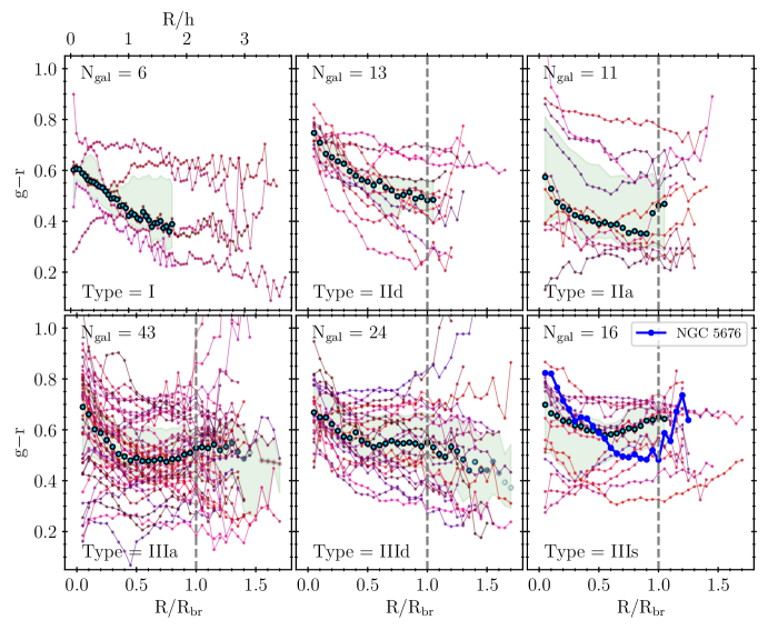
Figure 5: $g-r$ color profiles of sample galaxies, with radii normalized by the radius of the outermost break. In the case of Type I galaxies, the profiles are normalized instead by the disk scale length. Curves and points in shades of red through purple denote individual galaxy profiles, with the total number of profiles in each panel given as N_gal. Light blue points denote the median of all profiles at each radial bin, with the interquartile range (IQR) shown as the light green shaded region. For panels with N${}_{\rm gal}<20$, we show the median values and IQRs only where all galaxies contribute; for those with N${}_{\rm gal}>20$, marker transparency is calculated as the number of contributing galaxies at that radial bin divided by N_gal. The blue curve in the lower right panel shows the color profile of NGC 5676, the only Type IIIs galaxy in our sample with an extended blueward color gradient (see text).

Following Bakos et al. (2008), we show in Fig. 5 median $g-r$ color profiles of the galaxies in our sample, separated by outermost break type. Small multi-colored points in each panel show individual galaxy profiles, normalized by the outermost break radius R_br (and the disk scale length, in the case of Type I galaxies), while large light blue points show the running median, with the interquartile range (IQR) for all galaxies shown as the green shaded region. We truncate these median profiles for panels with fewer than 20 galaxies to the maximum radius of the shortest profile, as beyond this point the median values at each radial bin are misleading given the very small number of profiles contributing. For panels with more than 20 galaxies, the fewer the number of contributing galaxies at each radial bin, the more transparent the point. We note that for all break types, $g-i$ color profiles show the same behavior as these $g-r$ profiles, despite significantly higher background noise in the $i$-band images.

Given the lack of galaxies contributing to the median profiles for most break subclassifications, it is difficult to assess common trends. Type I profiles, for example, show a wide variety of behaviors: two galaxies trend continually blue, another trends blue but flattens beyond $\sim$2$h$, one trends blue only beyond $\sim$2$h$, and one more is roughly flat throughout. The median profile is therefore not reflective of the individual galaxy behaviors. However, Type IId galaxies show more consistent behavior, with the majority trending blue up to the break radius (as denoted by the median profile). Only one Type IId galaxy (NGC 3177) shows a distinct U-shaped profile akin to the average profiles of Type II disks found by Bakos et al. (2008); Zheng et al. (2015). In our galaxies, most of our outermost Type IId breaks occur at such low surface brightness that color information is not available much beyond R_br. Similarly, while the median profile for Type IIa galaxies shows a rough U-shape, the individual galaxy profiles show primarily either steadily blueward gradients, flat blue profiles, or blue inner disks with redward gradients in the outer disk. In the latter cases, the outermost redward gradients begin at roughly the break radius. Again, in only one case, NGC 5774, does the profile show a clear U-shape with a turnaround at the break radius. While it is encouraging that in several cases these downbending breaks, despite occurring at large radii and low surface brightness, appear to mark a star formation threshold like their higher surface brightness counterparts in other studies (Bakos et al. 2008; Zheng et al. 2015), deeper multiband imaging is clearly required to determine whether or not this is true for most of the galaxies in our sample.

Trends are more robust for Type IIIa and IIId galaxies given the larger sample sizes. Type IIIa disks show on average initial blueward gradients followed by fairly flat profiles averaging $g-r\sim$0.5. The radial extent of this bluer outer disk relative to the disk break in Type IIIa galaxies may be greater than that of Type II galaxies simply by definition: for example, the breaks in Type IIa disks mark the peak surface brightness of asymmetric features, while the breaks in IIIa disks mark the onset. If such galaxies are tidally interacting, this may also in many cases have resulted in elevated outer disk star formation rates, leading to sustained blue colors on average in the outskirts compared to typical Type IId galaxies (including possibly the Type IId galaxies in this study, if their steady blueward gradients also turn around at the break radius), modulo any extinction from dust.

Type IIId galaxies show decreasing color profiles on average, save a plateau between R$/$R${}_{\rm br}=0.5$–$1.0$, with $g-r\sim 0.7$ in their cores and $g-r\sim$0.4 in their outskirts. This color range is similar to the profiles of the Type IId galaxies inside of the break radius. If indeed the Type III breaks in these galaxies arise due to extended star formation or spiral arms, one might therefore expect many of these galaxies to eventually show a Type IId break (and red color upturn, potentially) in their outskirts as well, which the S⁴G and SDSS imaging is simply too shallow to locate.

Finally, the average color profile of Type IIIs galaxies appears much flatter than those of other types, with on average redder outer disks ($g-r\sim$ 0.6). While the disk colors of the individual IIIs galaxies display significant heterogeneity beyond $\sim 0.5$R_br, inside of this radius the profiles are split into two groups: those with $g-r\sim 0.4\pm 0.1$ (6 galaxies), and those with $g-r\sim 0.7\pm 0.1$ (10 galaxies). All of the galaxies with blue inner regions eventually show redward color gradients, albeit with different slopes and starting radii. Only one Type IIIs galaxy shows an extended blueward color gradient (NGC 5676, shown as a blue curve in Fig. 5), though even this galaxy shows a red upturn beyond R$/$R${}_{\rm br}\sim 1$.

4.3 Environmental correlation

Using our new break classification system, we test for correlations between break type and the local density of galaxies. Again, we test this using only the outermost breaks in each galaxy, which should be the most sensitive to the local environment.

4.3.1 Environmental Parameters

We compared breaks types using three measures of the local density. First, we use (as measured by Laine et al. 2014) the Dahari parameter $Q$ (Dahari 1984), a measure of tidal strength, and $\Sigma_{N}^{A}$, the projected surface number density within the $N^{\rm th}$ nearest-neighbor distance (Dressler 1980; Cappellari et al. 2011). Briefly, $Q$ is defined as:

$$Q_{i}=\frac{(D_{\rm p}D_{\rm c})^{\gamma}}{S^{3}}$$ (4)

where $D_{\rm p}$ and $D_{\rm c}$ are the diameters of the primary and companion galaxies, respectively, $S$ is their projected separation, and $\gamma=1.5$ (Rubin et al. 1982; Dahari 1984; Verley et al. 2007; Laine et al. 2014), and $\Sigma_{N}^{A}$ is defined as:

$$\Sigma_{N}^{A}=\log_{10}\left(\frac{N_{\rm gal}}{\pi R_{N}^{2}}\right)$$ (5)

where $N_{gal}=N=3$ and $R_{N}=R_{3}$ is the projected distance to the third nearest neighbor. For details, we refer the reader to Laine et al. (2014).

Finally, we also measure the surface number density within the galaxy groups defined by Kourkchi & Tully (2017) (hereafter, KT17), using the group’s second turnaround radius (Equation 6 of KT17, using the $K_{s}$ magnitude to estimate mass) to define the group surface area. We thus define this surface number density as:

$$\Sigma_{KT17}^{A}=\log_{10}\left(\frac{N_{\rm group}}{\pi R_{2t}^{2}}\right)$$ (6)

where $N_{\rm group}$ is the total number of members of the group to which the break-hosting galaxy belongs, and $R_{2t}$ is the group’s second turnaround radius. We use this surface density as an independent check against $\Sigma_{3}^{A}$, which measures density on quite local scales (e.g., Cappellari et al. 2011). For details on how these groups were defined, we refer the reader to KT17.

4.3.2 Statistical Tests

Given that we are performing comparisons of the means of environmental parameters between small sample populations (175 total galaxies split unevenly into 7 separate categories), we require a statistical test with more interpretive power, such that it minimizes the false-negative (type II error) rate. We therefore choose to perform a Bayesian comparison of means, using the method described by Kruschke (2013), dubbed BEST (for Bayesian Estimation Supersedes the T test). This method is a Bayesian corollary to Student’s t test (Student 1908), where the means and standard deviations are compared by their posterior distributions via Bayes’ formula:

$$p(\mu_{1},\sigma_{1},\mu_{2},\sigma_{2},\nu|D)=p(D|\mu_{1},\sigma_{1},\mu_{2},\sigma_{2},\nu)\cdot p(\mu_{1},\sigma_{1},\mu_{2},\sigma_{2},\nu)$$ (7)

for observations $D$, with $\mu_{1},\sigma_{1}$ the mean and standard deviation of population 1, $\mu_{2},\sigma_{2}$ the mean and standard deviation of population 2, and $\nu$ the number of degrees of freedom (as well as a normalization term, not shown). In the right-hand side of Equation 5, the first term is the likelihood and the second term is the prior (described in detail below).

To test for differences between galaxy populations, we use this method to compare the posterior distributions of the difference of means $\Delta\mu\equiv\mu_{1}-\mu_{2}$ of each environmental parameter, evaluated between all possible pairs of samples (21 comparisons for each environmental parameter). In each comparison, we adopt Gaussian priors on the population means (with prior means equal to the measured sample means), a wide uniform prior $U(0,5\sigma_{\rm tot})$ on the population standard deviations (with $\sigma_{\rm tot}$ the pooled standard deviation of the environmental parameter for the full 175 galaxy sample), and an exponential prior on $\nu$ of $\exp[-(\nu-1)/\lambda]$ with $\lambda=29$, as recommended by Kruschke (2013) as a balance between nearly normal distributions ($\lambda>30$) and distributions with heavy tails ($\lambda<30$). We find through experimentation with model Gaussian distributions that the results of the test are robust to the choice of priors, save that the use of too narrow priors on the standard deviations can result in posterior distributions of the means that are not reflective of the input simulated data. We assess the confidence level of each comparison using the cumulative probability of the posterior (hereafter, CP) up to a value of $\Delta\mu=0.0$ (a value that implies no difference in means). For example, if 90% of the posterior distribution on $\Delta\mu$ lies below 0.0 and only 10% above it, we may say with $\sim$90% confidence that $\Delta\mu<0.0$. A value of CP$=50$%, by contrast, implies no difference in populations. We show an example in Fig. 6, which implies that, with 95% confidence, Type IId galaxies are found in lower density environments than Type IIIs galaxies, if one measures density using $\Sigma_{3}^{A}$.

4.3.3 Results of Statistical Tests

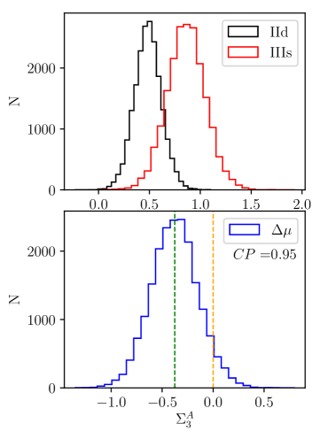
Figure 6: Demonstrating the posterior distributions of the mean vs. that of the difference in means, using the BEST method (see text). Top: the posterior distributions of the mean third nearest neighbor surface density $\Sigma_{3}^{A}$ for galaxies with outermost breaks of Type IId and IIIs. Bottom: the posterior distribution of the difference in the mean $\Sigma_{3}^{A}$ between Type IId and IIIs galaxies. The green dashed line shows the median of this distribution, while the orange dashed line shows $\Delta\mu=0.0$. The means differ by $\sim$1.7$\sigma$, and likewise the posterior distribution of $\Delta\mu$ peaks below 0.0 with $\sim$95% confidence.

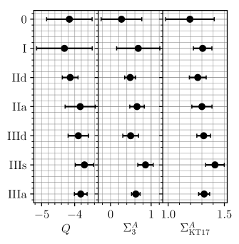
Figure 7: The means by outermost break type of three different environmental parameters. Error bars are the standard deviations of the posterior distributions of the means, following the BEST method (see text). The environmental parameters are, from left to right: Dahari $Q$, third nearest neighbor surface number density, and surface number density within the galaxy groups defined by KT17 (see text for full explanations).

In Fig. 7, we show the means of all three environmental parameters for galaxy populations separated by their outermost break type. The errorbars show the standard deviations of the posterior distributions of these means, following the BEST analysis (not the sample standard deviations). Though intragroup differences among these environmental parameters are small, we do find significant trends. Specifically, using all three environmental parameters, we find consistently that Type IIIs galaxies occupy the highest density environments, and either Type IId or 0 occupy the lowest density environments (although the uncertainty for Type 0 galaxies is very high given the small sample size, $N=6$). Additionally, Types IIa and IIIa typically show quite similar means, although the standard deviations are large for Type IIa.

In the interest of brevity, we showcase here only the strongest trends. Consistently, we find that Type IId galaxies occupy lower density environments than Type IIIs galaxies (CPs of 87%, 95%, and 92% for $Q$, $\Sigma_{3}^{A}$, and $\Sigma_{\rm KT17}^{A}$, respectively). This trend occurs even when using velocity limits on $Q$ and $\Sigma_{3}^{A}$ of 500 km s^-1, albeit at lower significance (CP $=$81% and 78%, respectively), suggesting it is robust. Indeed, Type IIIs galaxies may occupy higher density environments than all other break types, though at the lowest end (IIIs compared with IIa using $Q$) the CP is only 60%. Comparing a combined sample of Types I, IId, IIa, IIIa, and IIId against the IIIs sample gives CP$\sim$90% that IIIs galaxies occupy the densest environments.

A similarly robust trend is found regarding the Types IIa and IIIa, both of which appear to occupy similarly dense local environments (CPs of 52%, 56%, and 58% for $Q$, $\Sigma_{3}^{A}$, and $\Sigma_{\rm KT17}^{A}$, respectively). With lower confidence, we also find that Type IId galaxies occupy lower density environments than Types IIIa and IIa (CP $\sim$70–80%, or $\sim$85% using IIIa and IIa combined), suggesting that Type IId galaxies occupy some of the lowest density environments in our sample, including, potentially, with respect to IIId galaxies (CP $\sim$70%, though the comparison with $\Sigma_{3}^{A}$ suggests both populations occupy similar density environments). Finally, we find no significant trends regarding the Type I and 0 galaxies, though this may simply be due to their very low sample sizes (10 and 6, respectively).

As an alternative, we also performed pairwise comparisons using the Mann-Whitney U test (Mann & Whitney 1947). The trends regarding Types IId and IIIs remained insofar as tests comparing these break types consistently yielded the lowest p-values (with, again, Type IId galaxies seemingly occupying the lower density environments). However, these tests typically resulted in p-values $<0.2$ or $<0.1$, hence would not be considered significant under standard significance testing criteria (especially so if one chooses to correct for multiple comparisons). Therefore, while these comparisons are somewhat encouraging, these tests should be repeated using a larger sample size in order to verify these trends.

For now, a tentative summary follows: Type IId galaxies may occupy the lowest density environments, followed by Types IIIa and IIa, followed by Type IIIs, which occupy the highest density environments. Trends regarding the remaining break subtypes are ambiguous.

4.3.4 Break strengths

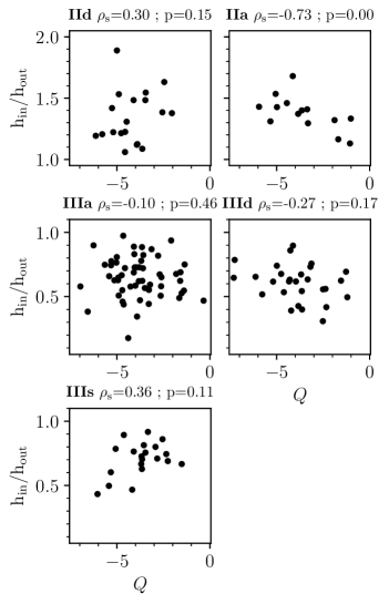
Figure 8: Correlations between break strength and the Dahari parameter (see text), separated by outermost break type. The values $\rho_{\rm s}$ denote the Spearman rank correlation coefficients for each comparison, while $p$ gives the p-value of the Spearman rank test.

As one final consideration regarding the origins of these disk breaks, we explore the correlation between environment and the outermost break strength by break subtype. We define break strength as the ratio of the disk scalelengths immediately preceding and following the outermost disk break, h${}_{\rm in}/$h_out (with scale lengths measured using the Numpy routine Polyfit; Oliphant 2006). We measure h_in between the outermost break radius inward to either the second to last break’s radius (if present) or to the inner radius boundary, and h_out between the outermost break radius and the outer radius boundary. Fig. 8 shows the correlation between the Dahari $Q$ parameter and the outermost break strength in each galaxy in our sample. For Type II breaks, higher values of h${}_{\rm in}/$h_out denote stronger breaks, while the inverse is true for Type III breaks.

As with our previous analysis of environmental parameters, the correlations we find between environment and break strength are subtle. Type IIa breaks show the strongest correlation, with Spearman rank correlation coefficient (Spearman 1904) $\rho_{\rm s}=-0.73$, i.e., stronger Type IIa disk breaks are found in lower density environments. This implies that the tidal features surrounding galaxies in lower density environments are morphologically sharper than those in higher density environments. Studies of the evolution of intragroup or intracluster light provide a feasible explanation for this, as tidal streams in higher density environments experience more frequent torques from passing galaxies and disperse more quickly (e.g., Rudick et al. 2009; Janowiecki et al. 2010). Type IIIa breaks, however, show no significant correlation with environment, despite many presumably arising through the same tidal mechanism as Type IIa breaks. In this case, the asymmetric nature of the host’s isophotes may explain this discrepancy: only those tidal features that align well with the choice of photometry aperture will have a well-measured scale length (or, indeed, will show a distinct down-bending break at the feature’s peak isophote).

Types IId and IIId show complementary behavior, such that stronger such breaks are found in higher density environments, however the trends here are quite weak ($|\rho_{\rm s}|\sim 0.3$) and not statistically significant (p-values $>0.15$). Therefore, while the local environment may influence these galaxies’ break strengths in measureable ways, despite them occupying the lowest density environments in our sample, the correlations are too weak to merit further discussion.

Break strengths in IIIs galaxies show a potential positive correlation with Dahari $Q$, implying stronger breaks in lower density environments, but again the correlation is small and not statistically significant ($\rho_{\rm s}\sim 0.36$, p-value $\sim 0.11$). This may imply that for IIIs galaxies, the boundary between the thin disk and the surrounding vertically extended component becomes weaker in denser environments, but this is again a tentative conclusion.

5 Discussion

5.1 Breaks, and what defines the outer disk

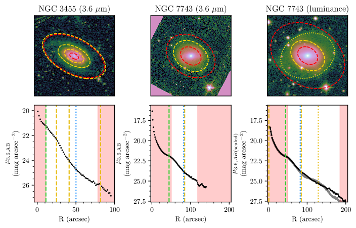
Figure 9: Galaxies ending in Type IIId disk breaks which seem to show faint Type IId breaks at larger radius. Ellipses, vertical lines, and shaded regions are as in Figures 1, 3, and 4. Left: NGC 3455 in 3.6$\mu$m, with mild evidence of a Type IId break occurring just beyond the galaxy’s faint outer spiral arms. Middle: NGC 7743 in 3.6$\mu$m, with no evidence of an outer Type IId break. Right: NGC 7743 in a luminance filter, converted roughly to 3.6$\mu$m AB magnitudes by scaling the surface brightness profile to the S⁴G profile at the 90% flux radius (image taken as part of the HERON survey; Rich et al. 2017). The image scale and surface brightness scale are the same as in the middle panels. Black points show the profile using the S⁴G isophotal parameters, which are clearly not representative of the outer disk; we therefore show a profile using a more appropriate position angle and ellipticity in gray points as well. Note that the outer disk contains an extremely faint outer ring, at the peak of which is a clear Type II disk break, when the correct isophote shape is used (dotted yellow ellipse and vertical line). The outer radius boundary here denotes where the black profile reaches the surface brightness of surrounding Galactic cirrus ($\mu_{3.6,\textrm{scaled}}\sim 27$; this cirrus also causes the additional Type III break near R$\sim$170″ in the gray profile).

By investigating the properties of outer disks using the properties of the outermost disk breaks of the host galaxies, we have implicitly defined the outer disk as that which exists beyond the last visible break radius. We feel this is a reasonable choice; it is more or less independent of surface brightness (thereby being defined similarly between normal spirals and, e.g., low surface brightness spirals; Impey & Bothun 1997), and a disk break, by definition, defines a lasting change in the properties of the disk. However, even by this definition, the “outer disk” demarcation necessarily depends on the depth of one’s data. While the S⁴G is the deepest survey of its kind (Sheth et al. 2010), disks in galaxies have been seen to extend beyond the $\mu_{V}=29$ mag arcsec^-2 isophote (e.g., Bland-Hawthorn et al. 2005; Vlajić et al. 2011; Watkins et al. 2016), several mag arcsec^-2 fainter than the limits of S⁴G (Sheth et al. 2010; Salo et al. 2015). It is therefore worth discussing the effects of the limiting surface brightness on this study, and by extension on all studies of disk breaks.

We can consider this from the perspective of all of the disk breaks we have identified. Because the S⁴G is fairly uniform in depth, but includes galaxies with a diversity of central surface brightnesses and scale lengths, if Type III breaks of a given subtype typically constitute the outermost breaks of their host, we have no reason a priori to suspect such breaks will typically be superseded by additional breaks at larger radius. By contrast, if Type III breaks of a given subtype were found to be frequently superseded by additional breaks within the survey’s photometric limits, this gives some reason to believe these breaks may also be frequently superseded by additional breaks below the survey’s photometric limits. Deeper imaging will, of course, be necessary to assess the validity of these assumptions, but they provide an initial guess.

Of all Type IIIs and IIIa breaks, 21/24 and 61/89 constitute the outermost breaks in their hosts, respectively (with 2/21 inner IIIs breaks followed by additional IIIs breaks, and 6/61 inner IIIa breaks followed by additional IIIa breaks). Thus, when these breaks occur, they tend to persist and so may most often truly demarcate the outer disks of their host galaxies. In that regard, it is noteworthy that of Type III breaks, Types IIIa and IIIs also appear to occupy the densest local environments (though again, these trends are fairly weak). By contrast, of 96 total Type IIId breaks identified in all galaxies in our sample, only 31 persist to the photometric limit of the data. In other words, the majority of Type IIId breaks we identify are immediately followed by some other type of break (most often of Type IId). Deeper imaging may therefore reveal that few, if any, Type IIId breaks persist indefinitely. These Type III breaks also showed the weakest correlation with environment, giving inconsistent results when comparing quite similar measures of the local surface number density of neighbors; this is expected if such breaks do not truly demarcate their hosts’ outer disks.

The question also arises whether or not our limit of three breaks per galaxy may be excluding some breaks beyond the outermost significant break uncovered by our algorithm. To this end, we re-ran the break-finding algorithm on all galaxies with three breaks, splitting the outermost profiles one additional time to seek out any significant breaks at larger radius. We uncovered such breaks in only two cases, therefore the limit of three breaks per galaxy does not affect our general conclusions.

If Type IIIa and IIIs breaks often constitute the outermost break in their hosts, is this also true of the outermost Type IId breaks we find? Previous studies hint that this may be the case: for example, in the four disk galaxies with extended Type II breaks observed by Watkins et al. (2014, 2016), the surface brightness profiles beyond these breaks showed no additional changes, to a limit of $\mu_{B}\sim 30$ mag arcsec^-2 (but see Trujillo & Fliri 2016). Each of these breaks were also coupled to the reversal of initially blueward color gradients in these galaxies, suggesting that Type II breaks followed by redward color gradients may often mark the outer disk radius in galaxies in which they are present. Indeed, the outer disks of such galaxies may be composed purely of scattered or radially migrated stars (e.g., Roškar et al. 2008; Schönrich & Binney 2009; Minchev et al. 2011; Roškar et al. 2012, and many others), with the break radius marking the extent of spiral structure and star formation. Most of the radial color profiles of our sample galaxies with extended Type II breaks did show similar initial blueward color gradients up to the break radius; however, deeper imaging is necessary to determine if such redward color gradients typically follow. We also found that galaxies with outermost breaks of Type IId appeared to occupy the least dense environments, a result aligning with that of Erwin et al. (2012), who found (albeit for S0 and Sa galaxies) that Type II breaks tend to vanish in clusters. Type IIa breaks may be similar, although the persistence of these breaks must depend on the presence or absence of additional tidal features or distortions present at larger radius.

In terms of representing the true “outer disk”, the outermost Type IIId breaks in our sample represent the most questionable cases, as a significant number of these may show additional breaks farther out. We show in Fig. 9 two illustrative examples: NGC 3455 and NGC 7743. In NGC 3455, extremely faint outer disk double spiral arms are visible in the S⁴G image, evidently the cause of the Type IIId break. However, a possible Type II break is visible in the surface brightness profile near $\sim$60″, just outside of our noise boundary radius, which aligns roughly with the outermost portions of both arms. NGC 7743 shows an even starker example; in the S⁴G image (central panel of Fig. 9), the only hint of outer spiral structure comes from two extremely faint ansae at the northeast and southwest sides of the visible disk (which occur just beyond the break radius). However, deep imaging of the galaxy from the Halos and Environments of Nearby Galaxies (HERON) survey (Rich et al. 2017) clearly shows two symmetric spiral arms emerging from the ends of these ansae, at the peak surface brightness of which is a very clear Type II break ($\sim 115$″; bottom-right panel of Fig. 9). This galaxy should therefore be classified as an oval galaxy of Type IId, with an outer disk offset nearly 90^∘ from the inner, presumably elliptical inner disk. None of this structure is visible in the S⁴G imaging, and only a hint of it is visible in SDSS imaging.

This is worth considering in any future disk break surveys. Particularly for surveys like SDSS, which do not probe to particularly deep surface brightness limits, Type IIId galaxies may prove a significant contaminant if one simply classifies breaks as Types I, II, and III, with no further consideration of these breaks’ possible origins. With these caveats in mind, we consider now the origins of Type III breaks in general.

5.2 The varying origins of Type III disk breaks

Of all galaxies with Type III breaks that persist to the photometric limit of our data, $\sim$53% are related to distorted isophotes or tidal features. In these cases, a radial profile assuming azimuthal symmetry is simply not an accurate representation of the true behavior of the galaxy’s isophotes. These disk breaks are therefore as much methodological in origin as they are physical in origin. This is reflected as well in the lack of correlation between Type IIIa break strength and the Dahari $Q$ parameter (Figure 8).

Given that such breaks are partly methodological in origin, one may question whether they should be considered as “disk breaks” at all (e.g., Pohlen & Trujillo 2006, in the case of their Type II-AB classification). We include them here for the sake of comparison with Laine et al. (2014) and L16, but it is clear that the scale lengths, break radii, and other physical parameters derived for these features depend strongly on the choice of aperture used to measure them. Particularly when seeking out correlations involving break strength, break radius, or similar parameters, such galaxies should always be classified separately. Regardless of their status as break-hosting galaxies, however, the source of their asymmetry is worth considering.

While in many cases the asymmetric nature of the Type IIIa break hosts is almost certainly the remnant of a tidal interaction or merger event (e.g., NGC 474, NGC 2782, NGC 4651, etc.), lopsidedness in galaxies need not always emerge through environmental influence (e.g., Zaritsky et al. 2013). That said, we have found that such distorted galaxies (of Types IIIa and IIa) may occupy denser local environments than all break type hosts but those of Type IIIs in this galaxy sample. We also found, for Type IIa galaxies, a strong anti-correlation between break strength and the tidal Dahari parameter $Q$. This is intuitive if such features are indeed most frequently tidal in origin: extended tidal streams preferentially form through low-speed, prograde encounters (e.g., Toomre & Toomre 1972; Eneev et al. 1973; Farouki & Shapiro 1982; Barnes & Hernquist 1992), such as might be more common in low-mass groups. Tidal features are also more easily disrupted and dispersed in denser environments (Rudick et al. 2009; Janowiecki et al. 2010), transforming previously sharp or shell-like tidal streams into more extended and diffuse streams. Therefore, we would expect to more often find these types of tidal signatures in galaxy pairs and groups than in either isolated or cluster galaxies.

Our firmest conclusion is that galaxies with outermost breaks of Type IIIs occupy the highest density environments. If these breaks mark the transition to vertically hotter galactic components, this is also intuitive. Galaxies occupying higher mass group or cluster halos should instead experience more frequent, higher velocity encounters (galaxy harassment; Moore et al. 1996) and ram-pressure stripping (Spitzer & Baade 1951; Gunn & Gott 1972), mechanisms capable of contributing to the morphology-density relationship (Spitzer & Baade 1951; Oemler 1974; Dressler 1980; Cappellari et al. 2011) by transforming spiral galaxies into lenticulars or ellipticals (e.g., Moore et al. 1996; Boselli & Gavazzi 2006; Cappellari et al. 2011). Strong and sustained such harassment would heat the host’s thin disk, thereby both expanding this surrounding spheroidal component and weakening the apparent boundary between this component and whatever remains of the thin disk. We see some evidence of this as well, in a possible correlation between break strength and $Q$ for Type IIIs galaxies (Fig. 8). The spheroidal components of many Type IIIs disk galaxies may thus be merely stellar populations tidally heated by such harassment, and therefore may represent examples of galaxies undergoing the transition from late to early type.

We may also see some evidence of this process in these galaxies’ color profiles, which are split between those with blue inner disks and redward color gradients, and those with red ($g-r\sim 0.7$) inner disks and flat, only slightly bluer ($g-r\sim 0.6$) outer disks. This behavior is reflected in these galaxies’ morphological types as well, which is bimodal: $11/21$ galaxies have T-types $\leq 2$, with the remainder $\geq$4, six of which are $\geq$8 (Buta et al. 2015). By contrast, the other break type hosts show roughly Gaussian T-type distributions peaking around $\sim$3 (though Type IIIa disks also show a sharp peak above 8), hence early type disks are relatively more prevalent among Type IIIs galaxies in this sample.

The gas in outer disks is vulnerable to both tidal forces (which may torque the gas, leading to infall; e.g., Barnes & Hernquist 1996; Hopkins et al. 2013) and ram-pressure stripping (Gunn & Gott 1972), both of which can deplete gas and truncate star formation in the outer regions of galaxies occupying dense environments. Gas that falls inward due to tidal torquing can go on to ignite central starbursts (e.g., Barnes & Hernquist 1991; Hernquist & Weil 1992; Barnes & Hernquist 1996; Cox et al. 2006; Hopkins et al. 2013), which may be the origin of those IIIs galaxies with blue central regions. If the gas is not replenished, sustained such interactions will deplete the galaxy’s reservoir and halt star formation. Rapid episodes of central star formation can increase both the central metallicity and dust content, leading to quite red integrated colors once star formation ceases. The two populations of Type IIIs galaxies in this sample may thus reflect galaxies currently undergoing quenching, and galaxies that have already quenched.

Simulations and observations suggest short quenching timescales, however (50 Myr – 2 Gyr for massive galaxies, e.g., Quai et al. 2018; Wright et al. 2018). At the upper end of these estimates, assuming typical ages of 10 Gyr, one might expect $\sim 20$% of any random population of galaxies undergoing quenching to still show significant star formation at $z=0$. In our sample, $6/16\sim$40% have blue inner disks, quite high even for this upper limit estimate. This suggests that other factors may be at play as well in the formation of Type IIIs disk breaks. The galaxies NGC 4800 and NGC 5676 provide interesting such examples: both galaxies appear as quite normal-looking star-forming disks embedded within a more diffuse, extended stellar envelope, and both galaxies show blueward color gradients that reverse at the IIIs break radius. These galaxies may instead represent galaxies with extended thick disks, following the suggestion by Comerón et al. (2012). If these thick disks arose during the early stages of these galaxies’ evolution (as is thought to be true of the Milky Way; e.g., Bensby et al. 2005), they need not be undergoing quenching at all. If this is the case, we would expect that with deeper imaging, the fraction of IIIs galaxies would increase, yet the correlation between IIIs breaks and environment may weaken, as only those Type IIIs breaks that occur at high surface brightness may be related to galaxy harassment and tidal interactions.

Previous work using the surface brightness profiles of S0 galaxies has also failed to find any difference in the Type III disk fraction between field and cluster environments (e.g., Erwin et al. 2012; Pranger et al. 2017; Sil’chenko et al. 2018). Several possibilities may explain this, in light of our conclusions here regarding Type IIIs galaxies. First, no distinction was made in these studies between Type III break subtypes, and Type IIIs breaks are relatively rare ($\sim$30% of all Type III breaks found in Erwin et al. 2012). Second, these studies made no distinction between the field and galaxy groups, only between galaxies inside and outside of clusters; the correlations between break subtypes and environment we find in our study are local. Third, many of the Type IIIs galaxies in our sample may not be transitioning into S0 galaxies, but into rotation-supported ellipticals. Differentiating among these scenarios to understand the origins of these Type IIIs galaxies will therefore require a much more detailed study, including detailed examination of stellar populations and kinematics.

The origins of Type IIIa and IIIs breaks thus appear diverse, but lean toward environmental influence. The remaining Type III galaxies in this sample are of Type IIId, suggesting their outer isophotes are dominated by extended, symmetric spiral arms or star-forming disks. Their color profiles appear to uphold this interpretation: most show roughly continual blueward color gradients (with a sharper downturn at the break radius; Fig. 5). This suggests a link between these galaxies and those of Type IId, which also often show blueward color profiles up to their own downbending break radii. However, the comparison between these populations’ local environmental density was ambiguous: in only one of three density parameters ($\Sigma_{3}^{A}$) did the two local environments appear similar.

While surface brightness limitations seem to play a role (as discussed in the previous section), some of this ambiguity may also be inherent to the classification of Type IIId galaxies itself. While Types IIIa and IIIs have quantifiable signatures (the $m=1$ Fourier mode amplitude and the isophotal ellipticity gradient, respectively), classifying Type IIId galaxies relies mostly on visual inspection and comparison across wavelengths. We also took a conservative approach to classification, labeling as part of the “disk” any largely symmetric spiral features, including those with large pitch angles that may be tidal in nature (e.g., NGC 2854, shown in Fig. 3).

Whether or not extremely faint, extended spiral arms like those of NGC 7743 (Fig. 9) are tidal in nature is also unclear. NGC 7743 itself does lie at roughly the same redshift distance as NGC 7742 (de Vaucouleurs et al. 1991), and is separated by only $\sim$50′ in projection ($\sim$320 kpc at 20 Mpc). NGC 7742 contains no bar, yet still hosts a star-forming nuclear ring (Comerón et al. 2010), as well as a counter-rotating gas disk (Sil’chenko & Moiseev 2006), implying a past merger event. These galaxies’ local environment thus is or recently has been somewhat active, implying the outer disk of NGC 7743 may also be tidal in origin. Two other galaxies in our sample with similar faint outer rings also have nearby companions: NGC 3684, near NGC 3607, and NGC 4151, near NGC 4145 (de Vaucouleurs et al. 1991). However, M94 (not in this sample), host to another oval and faint outer ring, is one of the most isolated galaxies in the nearby universe (Smercina et al. 2018). What we have labeled as “disklike” outer isophotes may therefore contain a mix of both secular features and tidal features, which are not easily distinguishable. Indeed, some breaks of this type may also result from a combination of secular processes and environmental interaction (e.g., Clarke et al. 2017; Ruiz-Lara et al. 2017). Again, this implies that the inclusion of Type IIId galaxies with other Type III galaxies will serve mainly to muddle any broad conclusions one may come to regarding the origins of Type III disks.

5.3 Implications for future work

The trends we have uncovered here, though weak, are promising. We have found multiple lines of evidence that the majority of upbending breaks in disk galaxy surface brightness profiles are indeed created through environmental influences, either through the creation of extended tidal features that skew the surface brightness profile at large radius (which may not be best characterized as “disk breaks”), or through merging or harassment in dense environments creating vertically hot, non-star-forming stellar components in the host disks.

Our current study, however, suffers from quite small sample sizes. This combined with any inherent subjectivity bias in our break categorization scheme — for example, our difficulty in differentiating symmetric tidal features from loosely wound outer spiral arms, as in the case of NGC 7743 described above — makes these conclusions still quite tentative. However, it is worth asking if such a detailed analysis is necessary to disentangle the competing influences on break formation in order to come to robust conclusions across studies regarding, e.g., the influence of secular vs. environmental processes on break formation. To test this, we applied the BEST analysis and the Mann-Whitney U test on the full dataset from L16, split generally into Type I, II, and III galaxies using these authors’ break classifications. We then performed pairwise comparisons between populations classified by break type (e.g., Type I vs. II, II vs. III, and I vs. III). In all comparisons save one, we found significant differences between populations’ mean Dahari $Q$ parameter or $\Sigma_{3}^{A}$ (at the $\gtrsim$95% confidence level), with Type III break hosts occupying the highest density environments. Only a comparison between Type III and II break hosts using the Dahari $Q$ parameter failed to uncover any significant difference using these broad categories. However, if we eschew all breaks from the Type II sample labeled II.i (denoting breaks inside the bar radius; Laine et al. 2014), we do find significant differences between the populations (CP $\sim$95%), with again Type III galaxies occupying the higher density environments. This suggests that the presence of disk breaks inside the bar radius are influenced far more by the presence of the bar than by any environmental factors, hence the inclusion of such breaks in a sample of Type II disk break hosts will again muddle any conclusions one may come to regarding the role of environment on disk break formation.

Some level of detail does therefore appear important regarding disk break classifications. In future studies of disk breaks, we therefore recommend specificity beyond simply identifying whether or not each galaxy hosts a Type II or Type III disk break at some radius. Depending on what physical scenarios are being explored using the disk breaks, perhaps this need not be as complex as what we have done in this study. Still, clarity should come through at least token effort at identifying the causal features behind the disk breaks one identifies, so that, to the best of one’s ability, environmental effects may be paired with environmental effects, and secular effects may be paired with secular effects. Also, one should be mindful that the “breaks” one is measuring are actually breaks and not simply a reflection of distorted isophotes. Doing otherwise risks cloudying already subtle correlations and scaling relations that might be illuminated by disk breaks.

6 Summary

We have re-analyzed the sample of Type III break-hosting galaxies first identified by Laine et al. (2014, 2016) in order to better understand the physical origins of Type III disk breaks.

Using an unbiased break-finding algorithm, we have reclassified the disk breaks in each of these galaxies and tied each significant change in slope to distinct features across the host disks. We find that, if one considers all breaks in all sample galaxies, Type III breaks are most frequently related to either morphological asymmetry (Type IIIa) or to features such as extended spiral arms or star forming regions (Type IIId). Many of the latter breaks, however, do not persist to the photometric limit of the data, typically being superseded by either asymmetry-related breaks, breaks associated with an outer spheroidal component (Type IIIs), or mild down-bending (Type II) breaks associated with, e.g., the ends of spiral arms (Type IId). Type III breaks associated with extended spiral structure or star formation (Type IIId), therefore, may not often truly characterize their hosts’ outermost disks.

We have analyzed the stellar populations of these galaxies using their $g-r$ color profiles, separating galaxies by outermost break type (the outermost break being the most sensitive to the local environment). We find that those galaxies with Type II breaks in their outskirts show blueward colors gradients up to the disk break radius; deeper multiband imaging is needed to determine whether or not these disks typically show redward color gradients beyond the break radius, as in Type II break galaxies from the studies by Bakos et al. (e.g., 2008); Zheng et al. (e.g., 2015). Galaxies with asymmetry-related breaks (Type IIIa) show flat and somewhat blue outskirts, possibly related to enhanced outer disk star formation caused by the asymmetry. Galaxies with outer spheroids (Type IIIs) show two distinct classes of color profiles: those with blue central regions and red outskirts, and those with red central regions and flat, only slighter bluer outskirts. This suggests that whatever mechanism has created the spheroids in these galaxies may also be related to quenching, with torqued gas falling inward, enhancing central star formation and enriching the core ISM in metals and dust. However, because the fraction of such galaxies with blue cores is too high compared to simulated populations of quenching galaxies, some of these outer spheroids may also be thick disks with extended scale lengths surrounding otherwise normal spirals.

Additionally, we compared the local environments of the various break-type hosts using three different parameters: the Dahari $Q$ parameter (a measure of tidal strength), and two measures of the local surface density (within the third nearest-neighbor projected radius, and within the groups defined by Kourkchi & Tully 2017). Though sample sizes are small, and therefore conclusions are still tentative, we find several consistent trends. We find that galaxies with outer spheroids (Type IIIs) seem to occupy the highest-density environments in our sample, suggesting again a connection between these components and, e.g., galaxy harrassment and quenching mechanisms. Along this line, we find a possible positive correlation between these galaxies’ break strengths and Dahari $Q$ parameter, suggesting that the boundary between the thin disk and the outer spheroid in such galaxies becomes weaker in denser environments. Galaxies with asymmetries (Types IIIa and IIa) appear to occupy the next highest-density environments, suggesting that most of these asymmetries are indeed related to tidal disturbances, albeit not as violent of tidal disturbances as those leading to the outer spheroids. Galaxies with down-bending breaks in their outskirts which seem associated with spiral arms or star-forming regions (Type IId) appear to inhabit the least-dense environments, suggesting that such breaks only persist in mostly undisturbed galaxies, a result in line with the near absence of Type II disks in clusters (Erwin et al. 2012). Finally, we find little concrete correlation between environment and those Type III breaks associated with spiral arms and extended star formation (Type IIId). We have shown that some of this ambiguity arises from insufficient surface brightness depth, as in several cases (most intriguingly, NGC 7743) we find that these galaxies’ outer disks show Type II breaks at lower surface brightness.

In general, most of those Type III disk breaks that occur in the outer disk appear to have arisen through environmental influences rather than secular evolution. Therefore, some distinction should be made in future studies regarding the physical origins of these breaks, specifically break location (inner disk vs. outer disk) and any associated morphological features (e.g., bars, spiral arms, tidal streams, or outer spheroids).

Appendix A The influence of systematics on surface brightness profiles

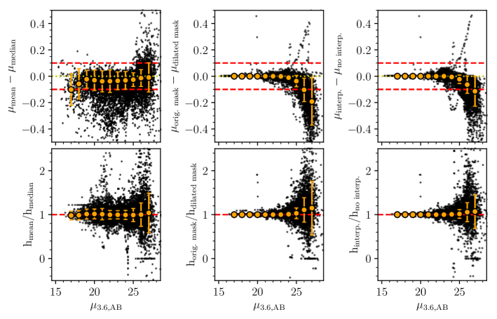
Figure 10: Showcasing systematic effects of different methods on the derivation of surface brightness as a function of radius, and local slope as a function of radius. Top row panels are, from left to right (all plotted as a function of surface brightness): difference between mean and median surface brightnesses; difference between surface brightnesses measured using the original S⁴G masks from Muñoz-Mateos et al. (2015) and those measured using dilated versions of the same masks; and surface brightnesses measured through interpolation across masks vs. those measured ignoring masked pixels. Bottom row panels show the same comparisons of systematics, but for the ratio of the measured local slopes (converted to scale length) using the varying methods. Orange points show the running median, with errorbars showing the interquartile range at each surface brightness bin. In the top row panels, red dashed lines show $\pm$0.1 mag arcsec^-2. In the bottom row panels, red dashed lines show a slope ratio of 1 (no difference between methods).

We explore here the effect of three different systematics on our measured surface brightness profiles: the choice of mean vs. median as the average flux in the radial bin, masking, and interpolation across masks vs. ignoring masked pixels. Fig. 10 shows a summary of the trends. In all panels, we plot the difference between methods as a function of surface brightness in black points, showing all measured surface brightnesses or scale lengths at all radial bins in all 175 sample galaxies.

A.1 Mean vs. median

In the leftmost panels of Fig. 10, we show the effects of using the mean vs. median surface brightness. We show the effect on surface brightness in the top-left panel. In general, the mean surface brightness is brighter than the median, such that $\mu_{\rm mean}-\mu_{\rm median}<0$. Regardless of surface brightness, this difference is $\sim-0.03$ magnitudes, with long tails to more extreme negative values (as large as half a magnitude in some cases). Below surface brightnesses of $\mu_{3.6,\textrm{AB}}\sim 25.5$, the scatter becomes symmetric and the median difference shifts closer to 0 (though is still slightly negative). This is roughly the limiting surface brightness of the S⁴G data, based on the uncertainty in the sky subtraction (Salo et al. 2015). At lower surface brightness, both mean and median begin to trace the peak of the background sky’s flux distribution (with a $\sim$0.01 mag arcsec^-2 skew to higher fluxes when using the mean), with large scatter. Where the galaxy’s light dominates the isophotes, then, the mean will tend to more closely trace the brightest features in the disk. In the sky-dominated regime, the mean will skew toward the brightest unmasked features (which, in the case of unresolved imaging, will usually be unmasked background galaxies or foreground stars; e.g., Rudick et al. 2010), and therefore is the more biased estimator at low surface brightness unless extreme care is taken to remove all sources of foreground or background contamination.

We show the effect of mean vs. median on the local slope in the bottom-left panel. We find no systematic effect on slope regarding the mean vs. median surface brightness, though again the scatter is large at all surface brightnesses. However, most of the outliers in this case skew to high values, implying that mean surface brightnesses, in extreme cases, tend to yield larger scale lengths. Unlike the effect on surface brightness, the effect on slope does not become symmetric below the noise limit. Likely this is due to the flux-weighted nature of the mean, which in these outlier cases tends more often to skew toward the brightest peaks in surface brightness, thereby leveling out the profile.

A detailed comparison of the mean vs. median profiles can be found on the website accompanying this paper (https://www.oulu.fi/astronomy/S4G_TYPE3_DISC_BREAKS/breaks.html). Median surface brightness profiles are included there alongside the mean profiles for each galaxy as gray dashed lines. We also provide these profiles in tabular form via CDS.

A.2 Masking

In the two center panels of Fig. 10, we display the effects of masking. In the top panel, we show the difference between surface brightnesses measured using the original S⁴G masks from Muñoz-Mateos et al. (2015) and those measured using the same masks but grown through dilation with a 3-pixel radius kernel. Down to roughly $\mu_{3.6,\textrm{AB}}\sim 24$ mag arcsec^-2, the measured surface brightnesses appear more or less insensitive to masking, on average (with IQR$<$0.01 mag arcsec^-2), though in individual cases the induced change can be as high as 0.1 mag arcsec^-2. At lower surface brightnesses, the masking begins to affect the profile systematically, with harsher masking resulting in fainter measured surface brightnesses and increased profile-to-profile scatter. By $\mu_{3.6,\textrm{AB}}\sim 25$, the median profiles have altered by $>$0.1 mag arcsec^-2, with a scatter of roughly the same value. Visual inspection of the images reveals that most of this effect can be attributed to the wings of the PSFs of bright stars leaking through masks, which artificially elevate the mean surface brightness measured in annuli where the galaxy isophotes are faint. We also find that the median, while more robust to masking, is not immune to this effect.

We show the effect of masking on the slope in the center-bottom panel. As discussed in Section 2, masking affects the slope profiles most at low surface brightness by increasing the measure scale lengths. The effect becomes strongest near $\mu_{3.6,\textrm{AB}}\sim 26$ mag arcsec^-2, though scatter is already significant at $\mu_{3.6,\textrm{AB}}\sim 25$. The overall influence of insufficient masking was to induce several spurious Type III breaks in our profiles, therefore we chose to include only those breaks that were not altered by the choice of mask. Again, use of the median over the mean alleviates but does not remove this effect. Proper masking is critical to measuring accurate surface brightness profiles at low surface brightnesses.

A.3 Interpolation across masks

Finally, in the rightmost panels of Fig. 10, we show the effect of our choice to interpolate across masks for this study. Interpolation was done primarily so that the surface brightness profiles could be used to measure the mass and potential of each galaxy as a function of radius (for example, for the purposes of measuring the influence of the bar; e.g., Díaz-García et al. 2016a, b). For the sake of comparison with Laine et al. (2014, 2016), we used the same surface brightness profiles, which included this interpolation. This, too, however, carries a systematic effect, such that interpolation artificially increases the surface brightness in a given radial bin. This effect is linked to the effect of masking, however; light leaking through masks carries through the interpolation, enhancing the surface brightness in the masked region. Use of more aggressive masks also removes this effect.

We show the effect of interpolation on the measured slopes in the bottom-right panel. Again, there is a slight systematic in the same direction as that induced by the masking. The root cause is again the same, therefore use of appropriately aggressive masks removes the systematic effects of interpolation as well.

In general, we find that these systematic effects alter our conclusions only in the low surface brightness regime, with masking and interpolation across masks showing the greatest influence. As discussed in Section 2, we have used only the larger masks in our analysis, thereby alleviating both of these biases. While individual galaxies can show extreme changes under these various systematics, overall the effects are quite small and so do not alter any of the conclusions we have discussed regarding populations of galaxies.