Some connections between the Classical Calogero-Moser model and the Log Gas

Abstract

In this work we discuss connections between a one-dimensional system of $N$ particles interacting with a repulsive inverse square potential and confined in a harmonic potential (Calogero-Moser model) and the log-gas model which appears in random matrix theory. Both models have the same minimum energy configuration, with the particle positions given by the zeros of the Hermite polynomial. Moreover, the Hessian describing small oscillations around equilibrium are also related for the two models. The Hessian matrix of the Calogero-Moser model is the square of that of the log-gas. We explore this connection further by studying finite temperature equilibrium properties of the two models through Monte-Carlo simulations. In particular, we study the single particle distribution and the marginal distribution of the boundary particle which, for the log-gas, are respectively given by the Wigner semi-circle and the Tracy-Widom distribution. For particles in the bulk, where typical fluctuations are Gaussian, we find that numerical results obtained from small oscillation theory are in very good agreement with the Monte-Carlo simulation results for both the models. For the log-gas, our findings agree with rigorous results from random matrix theory.

¹ Birla Institute of Technology and Science, Pilani - 333031, India

² International centre for theoretical sciences, Tata Institute of Fundamental Research,

Bangalore - 560089, India

1 Introduction

The study of systems of classical interacting particles in one-dimension (1D) with Hamiltonian dynamics is of interest from many points of view. From a dynamical point of view such systems are broadly classified as integrable and non-integrable and they are known to usually show qualitatively different behaviour when one looks at properties such as dynamical correlation functions, transport and equilibration. On the other hand as far as equilibrium properties are concerned one does not expect qualitative differences in behaviour arising out of integrability or otherwise of the Hamiltonian. Such finite temperature equilibrium properties of classical systems remains a subject of great interest till date. Seemingly unrelated systems often have common statistical properties and identifying universal features is one of the most interesting questions. Two very well-known one-dimensional models of interacting many particle systems are the so called log-gas (LG) and the Calogero-Moser (CM) model. The main aim of the present paper is a detailed study of the finite-temperature equilibrium properties of these two systems, pointing out surprising and unexpected connections between the two systems.

The log-gas model [1, 2] represents particles in 1D interacting with each other via a repulsive logarithmic potential and confined to move in a harmonic confining potential. The log-gas has a strong connection to random matrix theory [3, 4, 1]. The joint probability distribution function (pdf) of the eigenvalues of a $N\times N$ random matrix is given precisely by the equilibrium Boltzmann distribution of the positions of the $N$-particle log-gas [5, 1] — with the three important symmetry classes orthogonal, unitary and symplectic, of random matrices corresponding to $\beta=1,2,4$ in the log-gas distribution. Using this connection it has been possible to obtain many rigorous results for equilibrium properties of the log-gas at special values of the inverse temperature ($T^{-1}=\beta=1,2,4$) [6, 4, 1] while less is understood for other values of $\beta$ [1]. Some well known results include the single-particle distribution which is given by the Wigner semi-circle law and the marginal distribution of the edge particle given by the Tracy-Widom (TW) form [7, 8, 9, 10, 11, 2, 12]. Other results for the log-gas following from the random matrix connection include computation of density-density correlations [1, 13], and more recently it has been shown that the marginal distributions of $k<<N$ well-separated ordered bulk particles is Gaussian [14, 15, 16]. Somewhat surprisingly, although there have been several numerical studies [17] of Gaussian random matrix ensembles, the numerical simulation of the log-gas and numerical verification of various theoretical predictions are quite rare in the existing literature and in this paper we fill this gap.

On the other hand, the Calogero-Moser model [18, 19, 20, 21] describes a Hamiltonian system with particles interacting via a repulsive inverse square potential and confined in a harmonic potential. It is one of the classic examples of an integrable system, and apart from being an important solvable model in both classical and quantum physics, it has become ubiquitous in areas ranging from soliton physics, string theory, condensed matter physics, random matrix theory [22, 23, 24] as well as in pure mathematics. For the CM model, the integrals of motion can be constructed from Lax pairs [25, 26]. The model admits multi-soliton solutions and is known to display an interesting duality [27]. Although much has been studied in terms of collective field theory formalism [28, 29], nonlinear dynamics, solitons [27], quenches [30, 31] in the above model, the finite temperature equilibrium properties of the CM system are less well known. Connections with random matrix theory have also been noted. In [22] the Calogero-Moser potential (with harmonic pinning) was found to describe the eigenvalue distribution of a random matrix ensemble constructed from the Lax matrix of the Calogero-Moser Hamiltonian (without harmonic pinning potential). The level spacing distribution was found to be described by a form analogous to the Wigner surmise, but with very strong level repulsion. However other properties of the many-particle distribution were not investigated. In fact in contrast to the log-gas, there are few results on the equilibrium physics of the Calogero-Moser system.

At first sight the log-gas system and Calogero-Moser system appear to be quite unrelated but it turns out that unexpected connections between the two models have been noted. For the classical case, it was noted by Calogero [32] that the positional configuration of particles corresponding to the minimum of the potential is identical for both models and is given by the zeros of the Hermite polynomial. Furthermore it was pointed out that the Hessian matrices, corresponding to small oscillations around the minimum, are also related for the two models. In the quantum case, it was shown that the probability distribution corresponding to the ground state wave function of the Calogero-Moser model has a Boltzmann form with the potential being precisely that of the log-gas model [33, 34].

Given the several unexpected connections between the two models it is natural to explore this further in the context of classical equilibrium physics and this is the main aim of the present paper. An example of an interesting question that one could ask is regarding the distribution of the edge particle which is known to be of the Tracy-Widom form for the log-gas. In a recent paper the question of universality of this result for general 1D interacting systems was investigated and it was shown that the form is in fact very different for a 1D coulomb gas (interaction potential between particles given by modulus of distance) [35]. In the present paper we ask the same question for the Calogero-Moser model. More generally we explore other possible connections between the two models through a detailed study of their equilibrium correlations and various one-point distribution functions. We present results from extensive Monte-Carlo simulations of the two models as well as numerical computations from the Hessian matrices corresponding to small oscillations.

We summarize here our findings. We consider a system of $N$ particles with positions $(x_{1},x_{2},\ldots,x_{N})$ that are in thermal equilibrium at temperature $T=1/\beta$ in a many-body potential described by either the LG or the CM models. Our main results are:

(i) We verify that the single particle density distribution of the particles in both models converges in the continuum limit, as $N\to\infty$, to the Wigner semi-circle form at all finite temperatures, with differences from the log-gas in the finite-size effects.

(ii) For the CM model, we provide numerical evidence that the fluctuations of the edge particle $\delta x_{N}=x_{N}-\langle x_{N}\rangle$ scale as $\langle\delta x_{N}^{2}\rangle\sim N^{-2/3}$ in contrast to the well-known scaling form $\langle\delta x_{N}^{2}\rangle\sim N^{-1/3}$ for the log-gas. We find that the scaling function describing the typical fluctuations is non-Gaussian but different from the Tracy-Widom for $\beta=1,2,4$.

(iii) We compute marginal distributions of bulk particles $x_{k}$ with $1<<k<<N$ and find that they are Gaussian distributed with variances $\langle\delta x_{k}^{2}\rangle\sim 1/N$ for the CM model and $\langle\delta x_{k}^{2}\rangle\sim\log(N)/N$ for the LG model. For the LG model, we compare our results with the analytical predictions in [14, 15, 16].

(iv) We compute two-point correlations $\langle\delta x_{i}\delta x_{k}\rangle$ and verify the scaling form $\langle\delta x_{i}\delta x_{k}\rangle=(1/N)\leavevmode\nobreak\ f(i/N,k/N)$ where $f$ is a scaling function. This is valid except for $|i-k|<<N$, with different scaling functions for the LG and CM system.

(v) In all cases, we find that two-point correlations obtained from our Monte-Carlo simulations are in close agreement with the correlations obtained from the inverse of the Hessian matrices.

Our paper is organized as follows. In Sec 2, we define the two models, namely the log-gas and the Calogero-Moser systems and state some known results on their minimum energy configurations and the Hessian matrices corresponding to small oscillations around the minima. In Sec. 3, we present numerical results from Monte-Carlo simulations on various probability distributions and two-point correlation functions. The results on correlation functions are compared with earlier known rigorous results (for the log-gas) and with those obtained from inverse of the Hessian matrix (for both systems). We summarise our results along with an outlook in Sec. 4. Some of the numerical evidence demonstrating equilibration of the Monte-Carlo simulations are given in the appendix.

2 Model and summary of some known results

Here we first define the log-gas and the Calogero-Moser Hamiltonians. We consider a system of $N$ particles with positions $(x_{1},x_{2},\ldots,x_{N})$ and momenta $(p_{1},p_{2},\ldots,p_{N})$. The log-gas system is given by the following Hamiltonian:

$$H_{\rm log} =\sum_{i=1}^{N}\frac{1}{2m}p_{i}^{2}+V_{\rm log}(x_{1},x_{2},\ldots,x_{N}),$$

$${\rm where}\leavevmode\nobreak\ \leavevmode\nobreak\ V_{\rm log} =\sum_{i=1}^{N}\frac{1}{2}mw^{2}x_{i}^{2}-\sum_{i=1}^{N}\sum_{\begin{subarray}{c}j=1\\ j\neq i\end{subarray}}^{N}\frac{1}{2}\log|x_{i}-x_{j}|\leavevmode\nobreak\ .$$ (1)

This describes particles in 1D interacting via a logarithmic interaction potential and confined in a harmonic trap. For the Calogero-Moser system in a harmonic potential, the Hamiltonian is given by:

$$H_{\rm cal} =\sum_{i=1}^{N}\frac{1}{2m}p_{i}^{2}+V_{\rm cal}(x_{1},x_{2},\ldots,x_{N})$$

$${\rm where}\leavevmode\nobreak\ \leavevmode\nobreak\ V_{\rm cal} =\sum_{i=1}^{N}\frac{1}{2}mw^{2}x_{i}^{2}+\sum_{i=1}^{N}\sum_{\begin{subarray}{c}j=1\\ j\neq i\end{subarray}}^{N}\frac{1}{2}\frac{g^{2}}{(x_{i}-x_{j})^{2}}\leavevmode\nobreak\ .$$ (2)

This describes particles in 1D interacting via an inverse square interaction confined in a Harmonic trap. For studies of the equilibrium physics, the parameters $m,w,g$ can be scaled out and for the rest of the paper, we set $m=g=w=1$. Setting also Boltzmann’s constant $k_{B}$ = 1 the only relevant parameter is the inverse temperature $\beta={1}/{T}$.

2.1 Minimum energy configuration

The minimum energy configuration for the log-gas is given by the condition that the force $F_{i}$ on each particle vanishes:

$$F_{i}=-{\partial V_{\rm log}}/{\partial x_{i}}=-x_{i}+\sum_{\begin{subarray}{c}j=1\\ j\neq i\end{subarray}}^{N}(x_{i}-x_{j})^{-1}=0,\leavevmode\nobreak\ \leavevmode\nobreak\ \leavevmode\nobreak\ {\rm for}\leavevmode\nobreak\ i=1,2\ldots,N\leavevmode\nobreak\ .$$ (3)

It is well known that the solution for these set of equations is given by zeros of the Hermite polynomials $H_{N}(y)$ [13, 36], which we denote by $z^{(N)}_{i}$, for $i=1,2,\ldots N$. On the other hand the minimum energy configuration for Calogero-Moser model is given by the equation

$${\partial V_{\rm cal}}/{\partial x_{i}}=x_{i}-2\sum_{\begin{subarray}{c}j=1\\ j\neq i\end{subarray}}^{N}(x_{i}-x_{j})^{-3}=0,\leavevmode\nobreak\ \leavevmode\nobreak\ \leavevmode\nobreak\ {\rm for}\leavevmode\nobreak\ i=1,2\ldots,N\leavevmode\nobreak\ .$$ (4)

As was shown first by Calogero [37], it turns out that this equation is also satisfied by the Hermite zeros. Here, we present a simpler proof of this result.

We first note that the CM potential can be expressed in the form

$$V_{\rm cal}=\sum_{i=1}^{N}F_{i}^{2}/2+N/2\leavevmode\nobreak\ ,$$ (5)

with $F_{i}$ given in Eq. 3. This follows since

$$\sum_{i=1}^{N}F_{i}^{2} =\sum_{i=1}^{N}\left[x_{i}^{2}+\sum_{\begin{subarray}{c}j=1\\ j\neq i\end{subarray}}^{N}\frac{1}{(x_{i}-x_{j})^{2}}\right]+\sum_{\begin{subarray}{c}i,j,k=1\\ i\neq j\neq k\end{subarray}}^{N}\frac{1}{(x_{i}-x_{j})(x_{i}-x_{k})}-2\sum_{\begin{subarray}{c}i,j=1\\ i\neq j\end{subarray}}^{N}\frac{x_{i}}{(x_{i}-x_{j})}\leavevmode\nobreak\ .$$ (6)

The second term above can be symmetrized to give

$$\sum_{\begin{subarray}{c}i,j,k=1\\ i\neq j\neq k\end{subarray}}^{N}\frac{1}{(x_{i}-x_{j})(x_{i}-x_{k})} =\frac{1}{3}\left[\frac{1}{(x_{i}-x_{j})(x_{i}-x_{k})}+\frac{1}{(x_{j}-x_{k})(x_{j}-x_{i})}+\frac{1}{(x_{k}-x_{i})(x_{k}-x_{j})}\right]$$

$$=\frac{-(x_{j}-x_{k})-(x_{k}-x_{i})-(x_{i}-x_{j})}{(x_{i}-x_{j})(x_{j}-x_{k})(x_{k}-x_{i})}=0\leavevmode\nobreak\ ,$$ (7)

while the last term in Eq. (6) can be written as $\sum_{\begin{subarray}{c}i,j=1\\ i\neq j\end{subarray}}^{N}{x_{i}}/{(x_{i}-x_{j})}+{x_{j}}/{(x_{j}-x_{i})}=N$. Hence, we finally get

$$\sum_{i=1}^{N}F_{i}^{2}=\sum_{i=1}^{N}\left[x_{i}^{2}+\sum_{\begin{subarray}{c}j=1\\ j\neq i\end{subarray}}^{N}\frac{1}{(x_{i}-x_{j})^{2}}\right]-N\leavevmode\nobreak\ ,$$ (8)

which proves Eq. (5).

Differentiating Eq. 5 with respect to $x_{j}$, we get the force acting on a particle in the Calogero-Moser model:

$$-\frac{\partial V^{cal}}{\partial x_{j}}=-\sum_{i=1}^{N}F_{i}\frac{\partial F_{i}}{\partial x_{j}}\leavevmode\nobreak\ ,$$ (9)

which vanishes at $x_{i}=y^{(N)}_{i}$ since $F_{i}(y^{(N)}_{i})=0$. This proves that the zeros of $H_{N}(y)$ satisfy Eq. 4 and thus correspond to the minimum energy configuration of the CM potential.

2.2 Small oscillations and properties of Hessian matrix

The Hessian matrix describes small oscillations of a system about its equilibrium configuration ${\bf y}^{(N)}=[y^{(N)}_{1},y^{(N)}_{2},\ldots,y^{(N)}_{N}]$, and is defined for the log gas by

$$M^{\rm log}_{ij}=\left[\frac{\partial^{2}V^{\rm log}}{\partial x_{i}\partial x_{j}}\right]_{{\bf x}={\bf y}^{(N)}}=\delta_{ij}\left[1+\sum_{\begin{subarray}{c}k=1\\ k\neq i\end{subarray}}^{N}\frac{1}{(y^{(N)}_{i}-y^{(N)}_{k})^{2}}\right]-(1-\delta_{ij})\frac{1}{(y^{(N)}_{i}-y^{(N)}_{j})^{2}}\leavevmode\nobreak\ .$$ (10)

For the CM system, we get,

$$M^{\rm cal}_{ij}=\delta_{ij}\left[1+\sum_{\begin{subarray}{c}k=1\\ k\neq i\end{subarray}}^{N}\frac{6}{(y^{(N)}_{i}-y^{(N)}_{k})^{4}}\right]-(1-\delta_{ij})\frac{6}{(y^{(N)}_{i}-y^{(N)}_{k})^{4}}\leavevmode\nobreak\ .$$ (11)

Using the relation Eq. 5, it is easy to see that the Hessian matrices of the two models are simply related. Thus, one notes that,

$$\frac{\partial^{2}V^{cal}}{\partial x_{j}\partial x_{k}}=\sum_{i=1}^{N}\left[\frac{\partial F_{i}}{\partial x_{k}}\frac{\partial F_{i}}{\partial x_{j}}+F_{i}\frac{\partial^{2}F_{i}}{\partial x_{j}\partial x_{k}}\right]\leavevmode\nobreak\ .$$ (12)

Since the forces $F_{i}$ vanish at the minimum energy configuration ${\bf y}^{(N)}$, we immediately get $M^{\rm cal}_{jk}=\sum_{i=1}^{N}{\partial F_{i}}/{\partial y^{(N)}_{k}}{\partial F_{i}}/{\partial y^{(N)}_{j}}=[(M^{\rm log})^{2}]_{jk}$ and therefore, we get the following identity,

$$M^{\rm cal}=(M^{\rm log})^{2}\leavevmode\nobreak\ .$$ (13)

With this interesting connection between their Hessian matrices, it is expected then that Gaussian fluctuations and two-point correlation functions in the two models should be related. Let us denote,

$$S^{(C/L)}_{[i,j]}=\beta\braket{\delta x_{i}\delta x_{j}}\leavevmode\nobreak\ ,$$ (14)

where the superscript $C,L$ indicates CM or LG model respectively. From the small oscillations theory, we have,

$$S^{(C/L)}_{[i,j]}=[M^{\rm{cal/log}}]^{-1}\leavevmode\nobreak\ .$$ (15)

At the level of Gaussian fluctuations we can use the small oscillations approximation and, using the relation in Eq. (13), we arrive at the following relation between correlations in the two models:

$$S^{C}_{i,j} =\sum_{k=1}^{N}S^{L}_{i,k}S^{L}_{j,k}\leavevmode\nobreak\ .$$

For the LG there are some known exact results on two-point correlations and so it may be possible to use the above relation to arrive at some predictions for the CM model. We will explore some of these aspects in the following sections.

Before ending this section we note that the eigenvalues and eigenvectors of the Hessian matrices are known explicitly [32, 37] and we state their explicit forms. Let

$$H_{n}(x) =k_{n}\prod_{j=1}^{n}(x-x_{j})$$ (16)

$${\rm hence}\leavevmode\nobreak\ \leavevmode\nobreak\ H^{\prime}_{n}(x=x_{i}) =\left[\frac{\partial H_{n}}{\partial x}\right]_{x=x_{i}}=k_{n}\prod_{\begin{subarray}{c}j=1\\ j\neq i\end{subarray}}^{n}(x_{i}-x_{j})\leavevmode\nobreak\ ,$$ (17)

where $H_{n}(x)$ denotes the Hermite polynomial of order $n$ and $k_{n}$ is just a normalization constant. A column vector $\mathbf{v}^{(N)}$ is defined such that it’s $j^{th}$ element is

$$\mathbf{v}^{(N)}_{j}=\frac{1}{H^{\prime}_{N}(x_{j})}\leavevmode\nobreak\ ,\leavevmode\nobreak\ \leavevmode\nobreak\ j=1,2,\ldots,N\leavevmode\nobreak\ ,$$ (18)

while $\mathbf{X}^{(N)}$ is defined as a diagonal matrix with diagonal elements being set to be the $N$ zeros of $H_{N}(x)$. Then the eigenvectors of $M^{\rm log}$ (and naturally of $M^{\rm cal}$) are given by

$$\bm{\psi}^{(N)}_{j}=H_{j-1}(\mathbf{X}^{(N)}).\mathbf{v}^{(N)},\leavevmode\nobreak\ \leavevmode\nobreak\ j=1,2,\ldots,N\leavevmode\nobreak\ .$$ (19)

The eigenvalue corresponding to the $j^{\rm th}$ eigenvector $\bm{\psi}^{(N)}_{j}$ is $j$ for $M^{\rm log}$ and $j^{2}$ for $M^{\rm cal}$.

3 Numerical results for equilibrium properties

We now present various results on equilibrium properties of the two systems obtained from direct Monte-Carlo simulations. Most of our results are for the values $\beta=1,2,4$ of the inverse temperature.

We are particularly interested in:

(i) The particle density profile

$$P(x)=\frac{1}{N}\sum_{i=1}^{N}\langle\delta(x-x_{i})\rangle\leavevmode\nobreak\ ,$$ (20)

where $\langle...\rangle$ denotes an equilibrium average over the distribution $e^{-\beta V({\bf x})}/Z$.

(ii) The marginal distributions

$$P_{k}(x)=\langle\delta(x-x_{k})\rangle\leavevmode\nobreak\ ,$$ (21)

where $k=N$ (or $k=1$) refers to the edge particle and $1<<k<<N$ refers to bulk particles and the associated moments and cumulants of these distributions (mean, variance, skewness and kurtosis).

(iii) The two-point correlation functions $\langle\delta x_{i}\delta x_{j}\rangle$.

We also compute various properties from the small oscillations approximation. The small oscillation theory would predict that the mean position of the $k$-th particles is simply given by $y_{k}$ while correlation functions are given by the inverse of the Hessian matrix

$$M^{-1}_{i,j}:\equiv S_{[i,j]}\leavevmode\nobreak\ .$$ (22)

Note that this gives mean-squared-deviation of the $k$-th particle to be $S_{[k,k]}$.

Simulation approach: Note that here we are mostly interested in the properties of the system where particles maintain their ordering. This would normally require us to perform Monte-Carlo moves (single-particle displacements) of very small sizes so that particle-crossings are avoided, and this would make equilibration very slow. We avoid this issue by ignoring particle crossings during most of the Monte-Carlo steps but then ordering the particles during the data-collecting steps. The step-lengths were chosen so that acceptance was around $50\%$. In our simulatons we collect data after every $5$ Monte-Carlo cycles (each cycle involving $N$ attempts) and averages were typically computed with around $10^{7}-10^{8}$ samples. For marginal distributions and cumulants, the averages were computed over a larger ensemble with around $10^{10}$ samples for greater precision. Some checks on equilibration are shown in the appendix.

3.1 Density profile

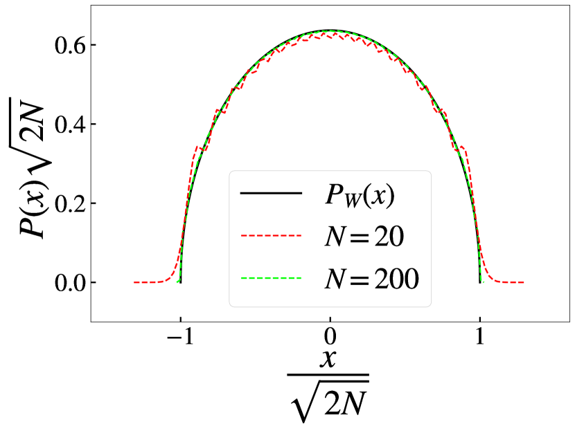
(a)

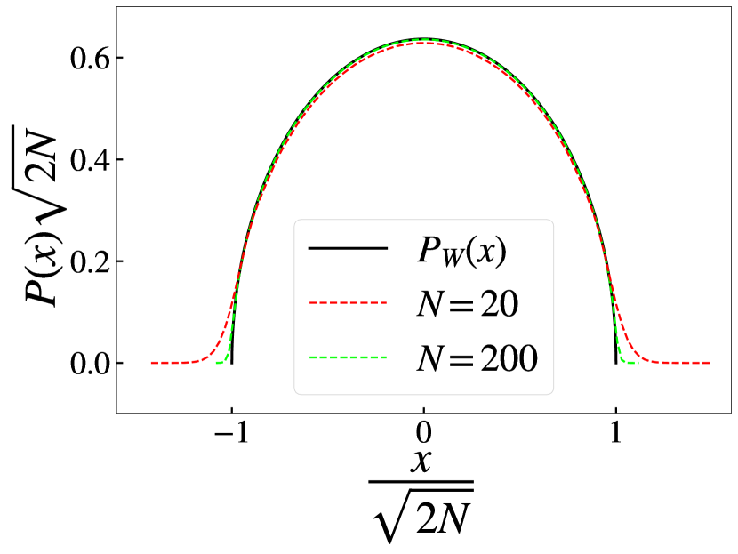
(b)

Figure 1: $P(x)$ versus $x$: Density of particles for $\beta$ = 4 for: (a) Calogero Model (b) Log-gas

Since the LG and CM have minimum energy configurations given by the Hermite polynomial zeros, it is expected that for low temperatures and in the thermodynamic limit, both the models will have single-particle distributions described by the Wigner semi-circle [38]

$$P_{W}(x)=\frac{1}{\pi}\sqrt{2N-x^{2}}\leavevmode\nobreak\ .$$ (23)

For the LG this is well known from random matrix theory and it has also been shown to be true for the CM model [27, 39]. We show in Figs. (1(a),1(b)), results from our simulations for $P(x)$ where we find that the agreement with $P_{W}(x)$ is good for finite systems even at high temperatures. We observe some deviations from the semicircle at the edges and this is due to finite-size effects. Note also the oscillations around the mean density profile that can be seen for the CM case. These oscillations, which decrease with increasing system size, indicate that the CM system is more rigid and that oscillations of particles around their mean position is smaller than in the LG.

3.2 Single-particle marginal distributions

3.2.1 Statistics of the edge particle position $x_{N}$

— In Figs. (2(a),2(b),3(a),3(b)) we show results for the mean position $\langle x_{N}\rangle$ and the variance $\langle\delta x_{N}^{2}\rangle$ of the edge particle. These are compared with the small-oscillation approximation results $y_{N}$ and $S(N,N)$ for the mean and variance respectively. From the properties of the Hermite zeros, it is known that the asymptotic value of $y_{N}$ is given by [40]:

$$y_{N}=\sqrt{2N}-\frac{\gamma}{(2N)^{1/6}}$$ (24)

where, $\gamma=1.8557$. From Figs. (2(a),2(b)) we see that for both the CM and LG model, the mean has the form

$$\langle x_{N}\rangle=\sqrt{2N}-\frac{c}{N^{1/6}}\leavevmode\nobreak\ ,$$ (25)

where the constant $c$ is temperature dependent, and approaches the constant $\gamma$, in the $\beta\to\infty$ limit. For the log-gas, it is known that the scaled variable

$$z=(x_{N}-\sqrt{2N})\leavevmode\nobreak\ kN^{1/6}\leavevmode\nobreak\ ,$$ (26)

with $k=2^{1/2}$ for $\beta=1,2$ and $k=2^{2/3}$ for $\beta=4$, satisfies the Tracy-Widom distribution $TW_{\beta}(z)$. Hence for the edge-particle mean in the log-gas, the limiting result $\lim_{N\to\infty}\langle z\rangle\to\langle z\rangle_{TW}$ is expected. Our numerics in Fig. (2(b)) verify this.

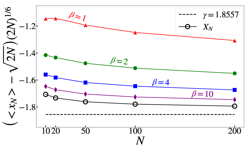
(a)

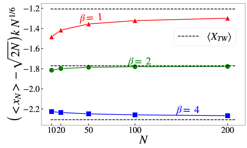
(b)

Figure 2: Plot of scaled mean displacement, from $\sqrt{2N}$, of the edge particle $x_{N}$, as a function of $N$, for (a) the CM model and (b) the LG model. For (a) we see that the low-temperature asymptotic value is close to the dashed line which is the value expected for the $N-$th zero of $H_{N}(y)$ in the large-$N$ limit. The rings, which denote exact values of the $N-$th zero of $H_{N}(y)$, approach the dashed line at very large-$N$. For (b) the asymptotic values are seen to approach the values expected from the TW distributions for $\beta=1,2,4$.

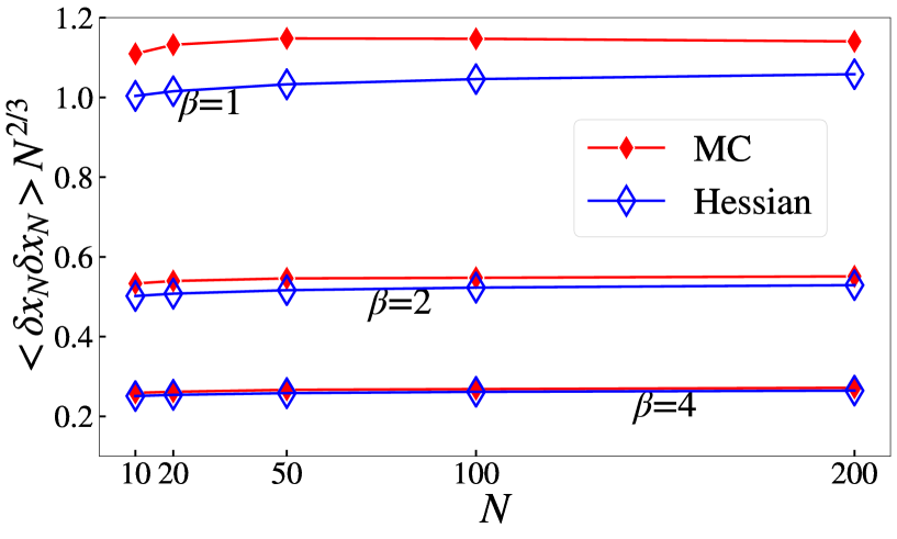
(a)

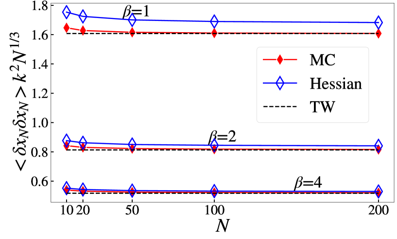
(b)

Figure 3: Plot of the scaled MSD of the edge particle $x_{N}$ plotted as a function of $N$ for (a) the CM model and (b) the LG model. The results from direct simulations and from the Hessian approach are shown and we see that they start differing at higher temperatures. However both predict the scaling $\langle\delta x_{N}^{2}\rangle\sim N^{-2/3}$ in the CM model and larger fluctuations $\langle\delta x_{N}^{2}\rangle\sim N^{-1/3}$ in the LG case. For the LG case we find the expected convergence of the MSD to the values obtained from TW.

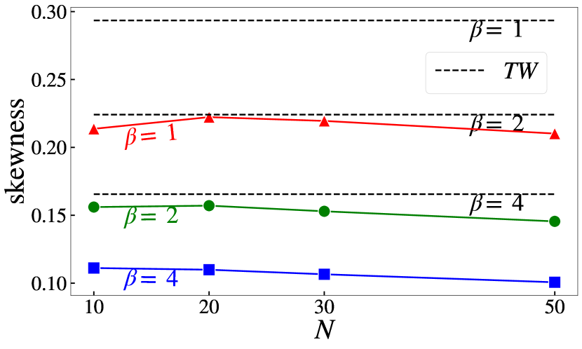
(a)

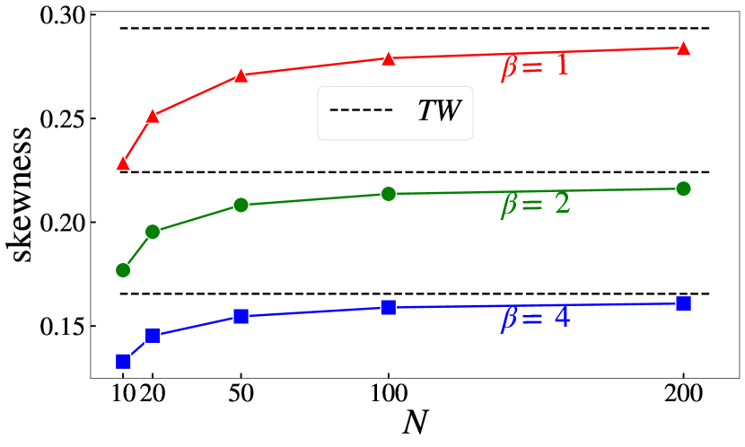
(b)

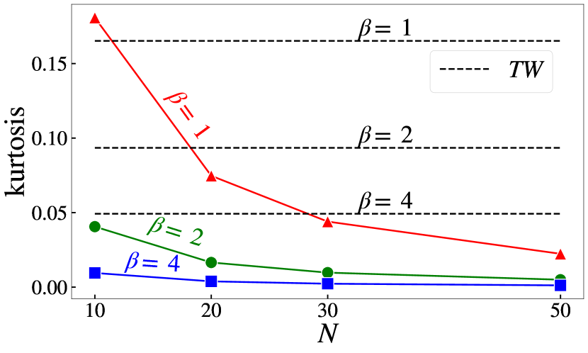
(c)

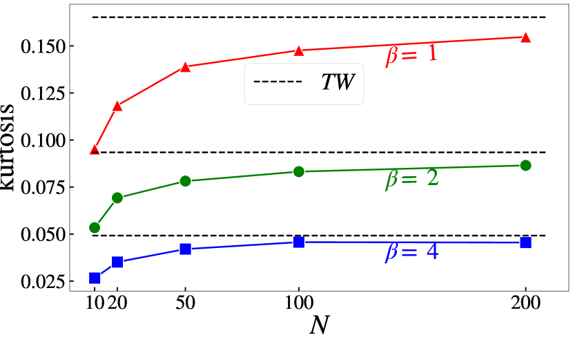
(d)

Figure 4: Figures (a) and (b) show plots of skewness versus system size for the CM and LG models respectively while figures (c) and (d) show plots of the kurtosis for the two cases. For the LG, we get the expected asymptotic values predicted by TW, while for the CM case it is clear that they differ significantly.

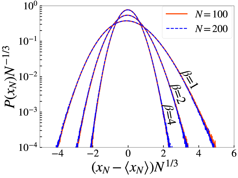
(a)

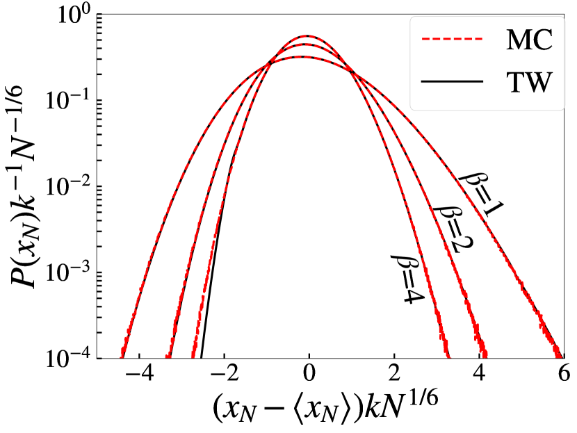
(b)

Figure 5: Full probability distribution of edge particle in (a) the CM model and (b) the LG, with appropriate scale factors. In (a) we show results for two system sizes $N=100,200$, and see good convergence indicating that we are already in the scaling limit. For (b) we only show the $N=200$ data since the $N=100$ scaled data is indistinguishable. We also find excellent agreement with the Tracy-Widom distribution over a wide range. The scale factors $k=2^{1/2}$ for $\beta=1,2$ and $k=2^{2/3}$ for $\beta=4$ are the standard ones for TW.

The fluctuations are much smaller in the CM model as compared with the LG. As shown in Figs. (3(a),3(b)), we find that

$$\langle\delta x_{N}^{2}\rangle\sim N^{-2/3}$$ (27)

for the CM, while the LG gives

$$\langle\delta x_{N}^{2}\rangle\sim N^{-1/3}\leavevmode\nobreak\ .$$ (28)

We have also plotted the results from the Gaussian theory and we see that these also reproduce the correct scalings, though not the precise prefactors. For the LG we have $\langle(z-\langle z\rangle)^{2}\rangle=(x_{N}-\langle x_{N}\rangle)^{2}\leavevmode\nobreak\ k^{2}N^{1/3}$ and this is again known from the variance of the Tracy-Widom. We verify this in Fig. (3(b)). A natural question is whether one can define an appropriately shifted and scaled variable, as in Eq. (26), which would satisfy the Tracy-Widom distribution. Since we do not have a theory which tells us what the shift and scale factors should be, it is not possible to test this from results on the mean and variance. However, the skewness and kurtosis of the distribution are quantities which are independent of both the shift and scale factors and computing these for the CM model gives us a direct way to test possible connections to Tracy-Widom. In Figs. (4(a),4(b)), we plot results for the skewness in the CM and LG respectively while in Figs. (4(c),4(d)) we plot the kurtosis in the two models. We find that while the LG results are consistent with that expected from Tracy-Widom, in the CM model we find that both quantities seem to decay with increasing system size, implying that the fluctuations are approximately Gaussian.

Full distribution of the edge particle $P_{N}(x)$: In Figs. (5(a),5(b)), we plot the full distributions of the edge particle position for the two models. For the LG model we find a very accurate verification of the TW distribution. On the other hand, for the CM model, the typical fluctuations appear to be Gaussian while the large deviations show significant asymmetry.

3.2.2 Statistics of bulk particle position $x_{N/2}$

For the log-gas, two-point correlations of the ordered particles have been computed exactly [15] and it has been shown that bulk correlations show Gaussian fluctuations. We summarize here the main results. It was shown that the the mean squared deviation of a bulk particle $1<<k<<N$ is given by

$$\braket{\delta x_{k}\delta x_{k}}=\frac{\log N}{2\beta[1-t^{2}(k)]N}$$ (29)

where $t(k)$ is to be found by inverting the relation

$$\frac{k}{N}=\frac{2}{\pi}\int_{-1}^{t}\sqrt{1-x^{2}}dx\leavevmode\nobreak\ .$$ (30)

It was also shown that correlations of bulk particles separated by distance $O(N)$ decay faster than $\log(N)/N$. From our numerics of the LG, we verify that the MSD of bulk particles scale as $(\log N)/N$. We also find that long-range correlations decay as $1/N$ (see next section). On the other hand for the CM, both the MSD and correlations decay as $1/N$. We now present the numerical results.

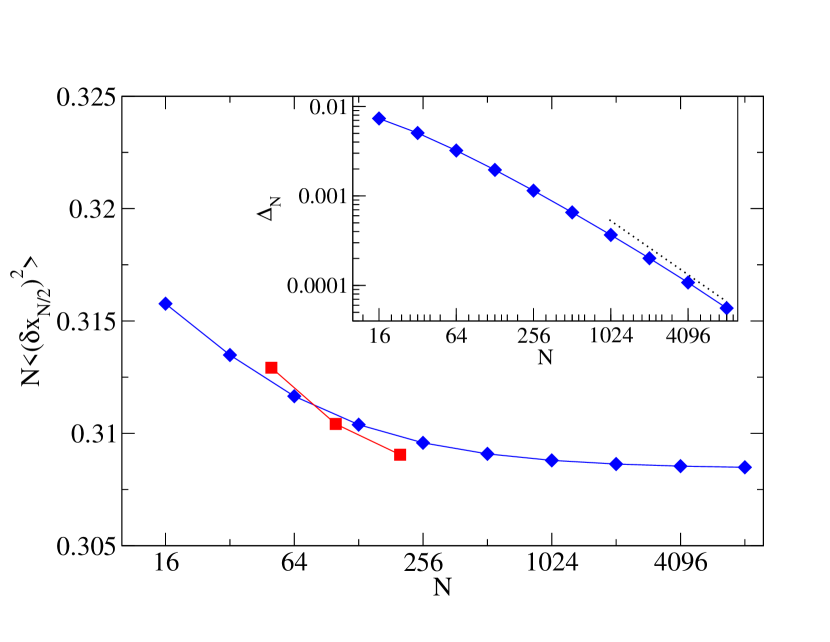
(a)

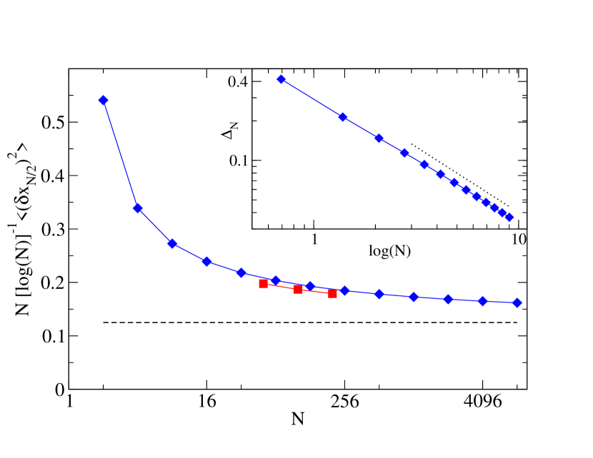
(b)

Figure 6: The scaled mean-squared-deviation in the position of particle $k=N/2$, as obtained from simulations (red squares) and from the Hessian (blue diamonds) for (a) the CM model and (b) the LG model, for $\beta=4$. For the LG model, we also show the expected theoretical prediction from Eq. (29) with the dashed line. For the CM model, the data fits well to the form $A+B/N$ with $A=0.3084$ and in the inset we plot, in log-log scale, $\Delta_{N}=N\langle\delta x_{N/2}^{2}\rangle-A$, which shows the $N^{-1}$ decay (dotted line). The inset in (b) in log-log scale shows the difference $\Delta_{N}=[N/\ln(N)]\langle\delta x_{N/2}^{2}\rangle-1/8$ (theoretical value) and we see a $[\log(N)]^{-1}$ decay (dotted line).

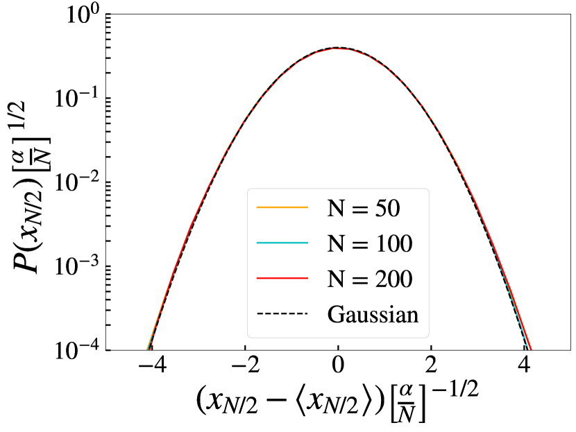
(a)

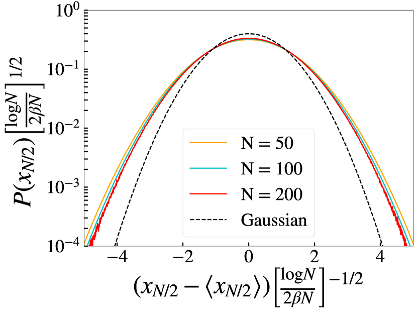
(b)

Figure 7: Probability distribution of $x_{N/2}$ obtained from simulations, for (a) CM model and (b) LG model, for three different system sizes $N=50,100,200$. For (a) we plot a Gaussian corresponding to the asymptotic MSD [see Fig. (6(a))] where $\alpha$ = A = 0.3084, and see a fast convergence of the simulation results to this form. For (b), we see a slow convergence to the expected theoretical Gaussian form for the LG.

In Figs. (6(a),6(b)), we plot the size-dependence of the mean-squared-deviations in the position of the $N/2$-th particles, for the CM and LG models respectively for $\beta=4$. Results of both direct simuations for sizes $N=50,100,200$, and the Hessian theory (where much larger sizes can be studied), are shown and we see good agreement between the two. For the CM model, there are no theoretical predictions and we find in Fig. (6(a)) that $\langle\delta x_{N/2}^{2}\rangle$ scales as $1/N$. In fact our data fits well to the form $N\langle\delta x_{N/2}^{2}\rangle=A+B/N$ with $A\approx 0.3084$ and the the inset shows a $\sim 1/N$ convergence to this asymptotic value. For the LG gas, using Eq. (29) with $k=N/2$ and $t(k=N/2)=0$, gives $N\langle\delta x_{N/2}^{2}\rangle/\log(N)=1/8$. We see in the inset of Fig. (6(b)) a slow convergence ($\sim 1/\log N$) to this limiting value. In Figs. (7(a),7(b)) we plot the full probability distributions, appropriately scaled, of the $N/2$-th particle. For the CM model we show the Gaussian form using the asymptotic variance $N\langle\delta x_{N/2}^{2}\rangle=0.3084$. For the LG we again see a slow convergence to the theoretically expected Gaussian distribution.

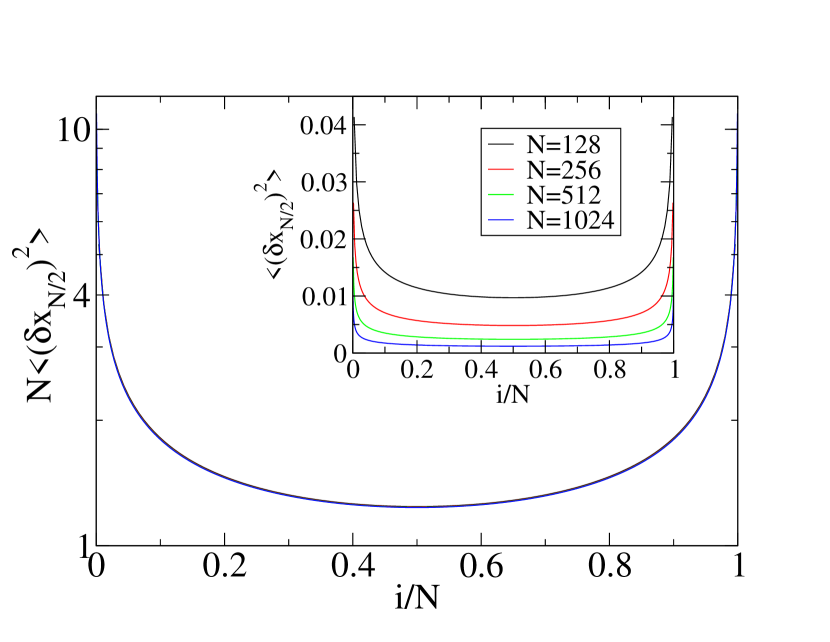
(a)

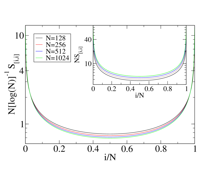
(b)

Figure 8: MSD profiles in (a) the CM and (b) the LG model, as computed from the Hessian, for different system sizes. In (a) we see a very good $1/N$ scaling while in (b) we show that a $\ln(N)/N$ scaling gives a better collapse than a $1/N$ scaling (inset).

In Figs. (8(a),8(b)), we show that the mean squared displacements at all bulk points, evaluated from the Hessian, also satisfy the $1/N$ and $\log(N)/N$ scaling for the CM and LG systems respectively.

3.3 Results on two-point correlations

Finally we present results on correlations in the fluctuations in the positions of the ordered particles, i.e., we look at $\langle\delta x_{i}\delta x_{k}\rangle$, where $\delta x_{i}=x_{i}-\langle x_{i}\rangle$. As stated in Eq. (14), in the small oscillation approximation, the two-point correlations are given by the inverse of the Hessian matrix. In Figs. (9) we compare results for correlations obtained from direct numerical simulations with those obtained from the Hessian, for $N=200$. It is clear that there is good agreement for both the CM and LG models.

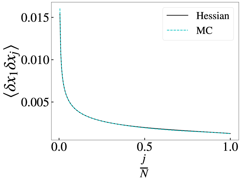
(a)

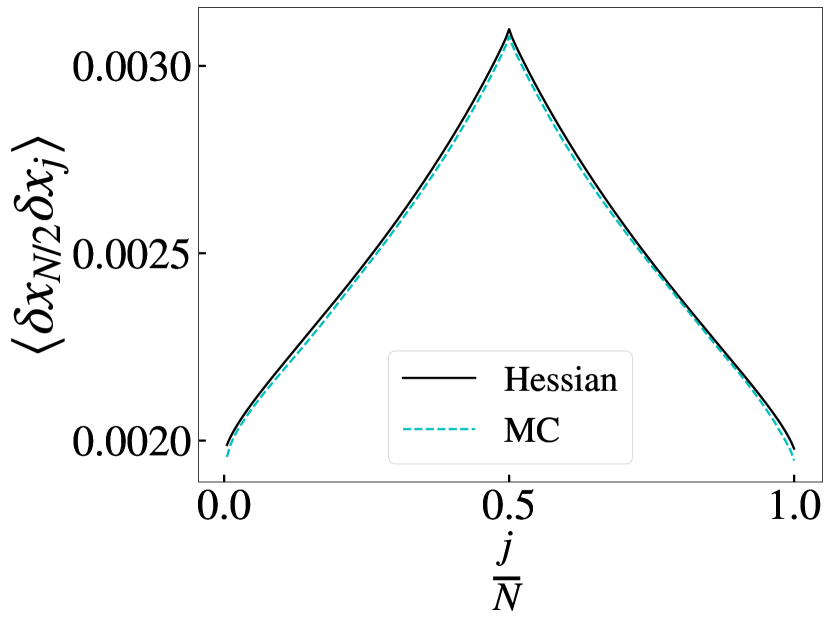
(b)

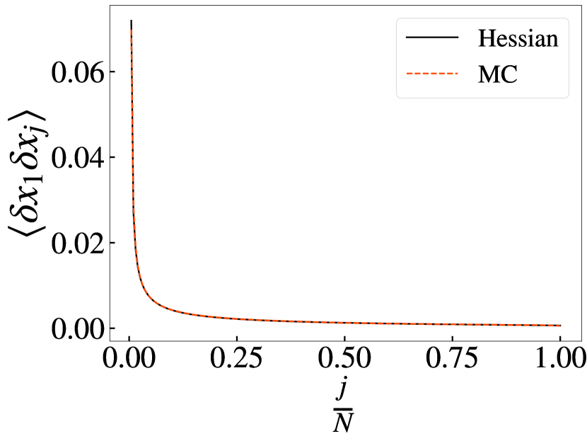
(c)

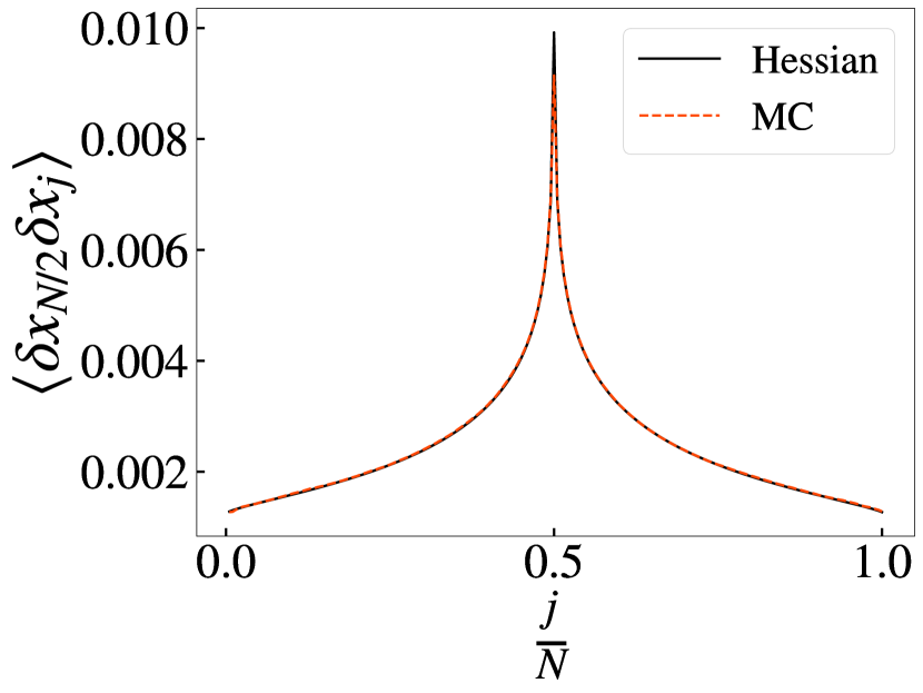
(d)

Figure 9: Comparison of correlations $\langle\delta x_{1}\delta x_{j}\rangle$ and $\langle\delta x_{N/2}\delta x_{j}\rangle$, obtained from MC simulations, with those obtained from the Hessian matrix, for (a,b) CM model and (c,d) the LG model at $\beta=2$ and $N=200$.

In Fig. (10) we present results from the Hessian matrix for different system sizes and find the following finite-size scaling form for both models:

$$S^{(C/L)}_{[i,j]}=\frac{1}{N}f\left(\frac{i}{N},\frac{j}{N}\right),$$ (31)

where $f$ is some scaling function. This has been shown for both Calogero and Log-gas models. As shown in the figure, for Calogero model this relation holds well at all particle positions. Near the edge particles, the relation breaks down. For Log-gas, this relation holds reasonably well when correlations are between particles separated by $\leavevmode\nobreak\ O(N)$ but breaks down for smaller distances.

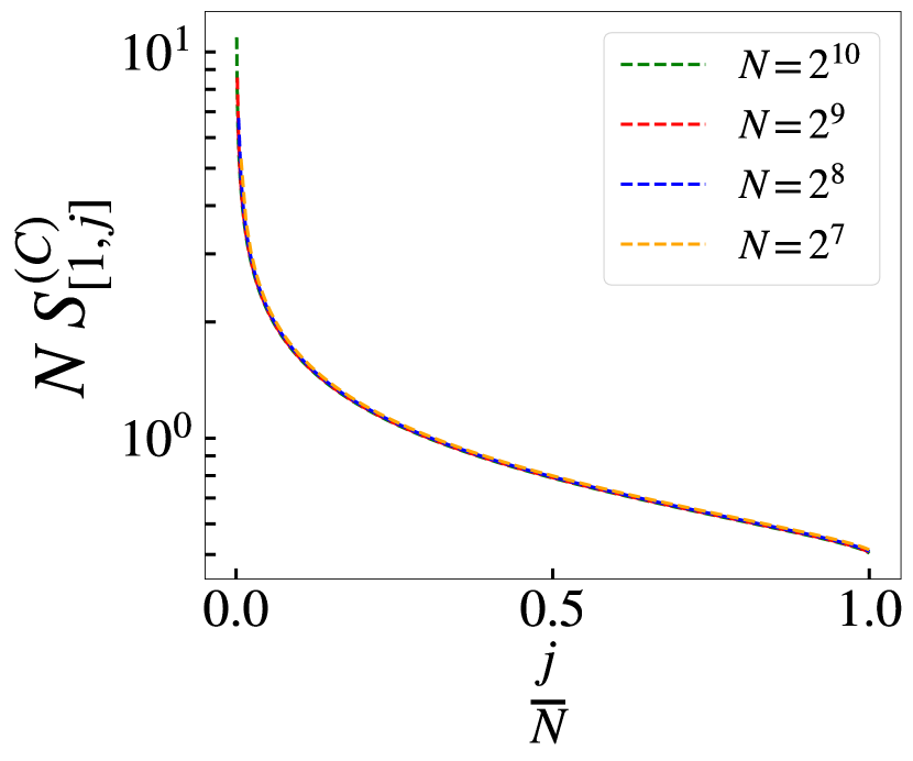
(a)

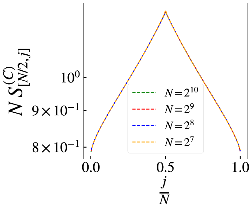
(b)

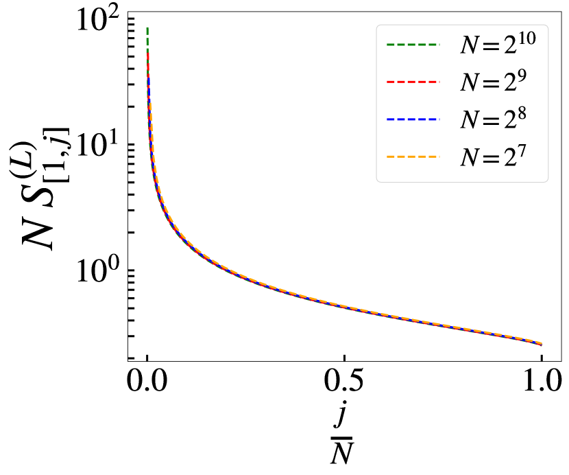
(c)

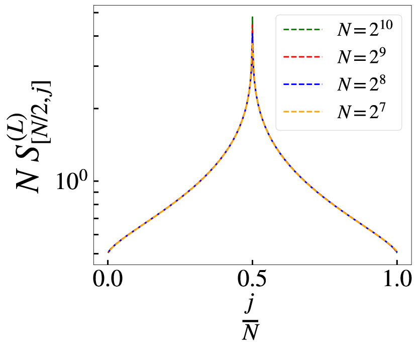
(d)

Figure 10: Plot of correlations $\langle\delta x_{1}\delta x_{j}\rangle$ and $\langle\delta x_{N/2}\delta x_{j}\rangle$ obtained from the Hessian matrix, for (a,b) the CM model and (c,d) the LG model. It is clear that the correlations satisfy a $1/N$ scaling

4 Conclusions

In this work we pointed out some connections between the log-gas (LG) and the Calogero-Moser (CM) model, two systems that have been widely studied in the context of random matrix theory and integrable models respectively. We looked at equilibrium properties of these two systems by performing extensive Monte-Carlo simulations to compute single-particle distribution functions of edge and bulk particles, and two-point correlation functions. We compared the Monte-Carlo results with those obtained from a Hessian theory, corresponding to making the approximation of small oscillations about the potential minima. We find that, except for the form of the distribution of the edge particle (which is non-Gaussian), the small oscillation approximation results are in general found to be in close agreement with the Monte-Carlo results. This includes results on non-trivial system-size scaling properties.

For the LG model, our Monte-Carlo simulations provide an accurate verification of the Tracy-Widom distribution at the parameter values $\beta=1,2,4$. For the CM model, we find a non-trivial scaling of the MSD for the edge particle, $\langle\delta x_{N}^{2}\rangle\sim N^{-2/3}$, as opposed to $\langle\delta x_{N}^{2}\rangle\sim N^{-1/3}$ for the LG. However, while we find that the distribution is non-Gaussian, it is distinct from the Tracy-Widom form seen in the LG. For the LG model, our MC simulations and Hessian theory computations results provide a verification of recent predictions [14, 15, 16] on single-particle distribution of bulk particles, including the $\log(N)/N$ scaling of the MSD. For the CM model we find that fluctuations of bulk particles are Gaussian, with a $1/N$ scaling of the MSD, and two-point correlations also have the same scaling. Some further interesting future directions would be the analytical computation of correlations from the Hessian theory for both models and the use of field theory approaches for the CM model to obtain analytical results.

5 Acknowledgements

We thank Anirban Basak, Manjunath Krishnapur, Anupam Kundu, Arul Lakshminarayan, Joseph Samuel, Herbert Spohn, Patrik Ferrari and Satya Majumdar for useful discussions. AD would like to acknowledge support from the project 5604-2 of the Indo-French Centre for the Promotion of Advanced Research (IFCPAR). MK would like to acknowledge support from the project 6004-1 of the Indo-French Centre for the Promotion of Advanced Research (IFCPAR). MK gratefully acknowledges the Ramanujan Fellowship SB/S2/RJN-114/2016 from the Science and Engineering Research Board (SERB), Department of Science and Technology, Government of India. SA would like to acknowledge support from the Long Term Visiting Students’ Programme, 2018 at ICTS. SA is also grateful to Aditya Vijaykumar and Junaid Bhatt for helpful discussions. We would like to thank the ICTS program “Universality in random structures: Interfaces, Matrices, Sandpiles (Code: ICTS/URS2019/01)” for enabling valuable discussions with many participants.

6 Equilibration and Convergence check

The most general form of the equipartition theorem states that under suitable assumptions, for a physical system with Hamiltonian $H$ and degrees of freedom $x_{n}$, the following holds in thermal equilibrium for all indices $m$ and $n$ [41]:

$$\left\langle x_{m}\frac{\partial H}{\partial x_{n}}\right\rangle=\delta_{mn}k_{B}T$$ (32)

This has been used to ascertain whether the system is at its equilibrium configuration, where $x_{i}$ is the position of $i^{th}$ particle. Using ergodicity, time average can be considered equivalent to ensemble average and hence, the above average is over microstates in the ensemble. Convergence check has been performed over different number of microstates (samples) to see if the number of samples is sufficient for averaging in statistics. We have found that the Calogero-Moser system converges at $16\times 10^{7}$ samples for $N=100,200$ and the Log-gas System converges at $8\times 10^{7}$ samples for $N=100,200$ as shown in Figure (LABEL:fig:virial). This figure demonstrates that our brute-force numerics are very accurate given the good agreement with the generalized virial theorem, which quantifies the equilibration of the system as given in equation (32).

References

- [1] Peter J Forrester. Log-gases and random matrices (LMS-34). Princeton University Press, 2010.
- [2] Taro Nagao and Peter J Forrester. Asymptotic correlations at the spectrum edge of random matrices. Nuclear Physics B, 435(3):401–420, 1995.
- [3] Paul Bourgade. Bulk universality for one-dimensional log-gases. In XVIIth International Congress on Mathematical Physics, pages 404–416. World Scientific, 2014.
- [4] László Erdos. Universality for random matrices and log-gases. arXiv preprint arXiv:1212.0839, 2012.
- [5] Yacin Ameur, Håkan Hedenmalm, Nikolai Makarov, et al. Fluctuations of eigenvalues of random normal matrices. Duke mathematical journal, 159(1):31–81, 2011.
- [6] Percy Deift. Universality for mathematical and physical systems. arXiv preprint math-ph/0603038, 2006.
- [7] Craig A Tracy and Harold Widom. Correlation functions, cluster functions, and spacing distributions for random matrices. Journal of statistical physics, 92(5-6):809–835, 1998.
- [8] Craig A Tracy and Harold Widom. The distributions of random matrix theory and their applications. In New trends in mathematical physics, pages 753–765. Springer, 2009.
- [9] Harold Widom. On the relation between orthogonal, symplectic and unitary matrix ensembles. Journal of Statistical Physics, 94(3-4):347–363, 1999.
- [10] Jinho Baik, Gérard Ben Arous, Sandrine Péché, et al. Phase transition of the largest eigenvalue for nonnull complex sample covariance matrices. The Annals of Probability, 33(5):1643–1697, 2005.
- [11] TH Baker and PJ Forrester. Finite-n fluctuation formulas for random matrices. Journal of statistical physics, 88(5-6):1371–1386, 1997.
- [12] Taro Nagao and Peter J Forrester. Transitive ensembles of random matrices related to orthogonal polynomials. Nuclear Physics B, 530(3):742–762, 1998.
- [13] Madan Lal Mehta. Random matrices, volume 142. Elsevier, 2004.
- [14] Jonas Gustavsson. Gaussian fluctuations of eigenvalues in the gue. In Annales de l’Institut Henri Poincare (B) Probability and Statistics, volume 41, pages 151–178. No longer published by Elsevier, 2005.
- [15] Sean O’Rourke. Gaussian fluctuations of eigenvalues in wigner random matrices. Journal of Statistical Physics, 138(6):1045–1066, 2010.
- [16] Deng Zhang. Gaussian fluctuations of eigenvalues in log-gas ensemble: Bulk case i. Acta Mathematica Sinica, English Series, 31(9):1487–1500, 2015.
- [17] Folkmar Bornemann. On the numerical evaluation of distributions in random matrix theory: a review. arXiv preprint arXiv:0904.1581, 2009.
- [18] F Calogero. Exactly solvable one-dimensional many-body problems. Lettere al Nuovo Cimento (1971-1985), 13(11):411–416, 1975.
- [19] Francesco Calogero. Solution of a three-body problem in one dimension. Journal of Mathematical Physics, 10(12):2191–2196, 1969.
- [20] Francesco Calogero. Solution of the one-dimensional n-body problems with quadratic and/or inversely quadratic pair potentials. Journal of Mathematical Physics, 12(3):419–436, 1971.
- [21] JURGEN MOSER. Three integrable hamiltonian systems connected with isospectral deformations. In Surveys in Applied Mathematics, pages 235–258. Elsevier, 1976.
- [22] E Bogomolny, Olivier Giraud, and C Schmit. Random matrix ensembles associated with lax matrices. Physical review letters, 103(5):054103, 2009.
- [23] Manas Kulkarni and Alexios Polychronakos. Emergence of the calogero family of models in external potentials: duality, solitons and hydrodynamics. Journal of Physics A: Mathematical and Theoretical, 50(45):455202, 2017.
- [24] Alexios P Polychronakos. The physics and mathematics of calogero particles. Journal of Physics A: Mathematical and General, 39(41):12793, 2006.
- [25] MA Olshanetsky and Askolʹd Mikhaĭlovich Perelomov. Classical integrable finite-dimensional systems related to lie algebras. Physics Reports, 71(5):313–400, 1981.
- [26] Askold Mikhailovich Perelomov. Integrable systems of classical mechanics and Lie algebras. Birkhäuser, 1990.
- [27] Alexander G Abanov, Andrey Gromov, and Manas Kulkarni. Soliton solutions of a calogero model in a harmonic potential. Journal of Physics A: Mathematical and Theoretical, 44(29):295203, 2011.
- [28] Inês Aniceto, Jean Avan, and Antal Jevicki. Poisson structures of calogero–moser and ruijsenaars–schneider models. Journal of Physics A: Mathematical and Theoretical, 43(18):185201, 2010.
- [29] Inaki Anduaga Michael Stone and Lei Xing. The classical hydrodynamics of the calogero–sutherland model. Journalof Physics A:Mathematical and Theoretical, 41, June 2008.
- [30] Fabio Franchini, Andrey Gromov, Manas Kulkarni, and Andrea Trombettoni. Universal dynamics of a soliton after an interaction quench. Journal of Physics A: Mathematical and Theoretical, 48(28):28FT01, 2015.
- [31] Fabio Franchini, Manas Kulkarni, and Andrea Trombettoni. Hydrodynamics of local excitations after an interaction quench in 1d cold atomic gases. New Journal of Physics, 18(11):115003, 2016.
- [32] F Calogero. Equilibrium configuration of the one-dimensionaln-body problem with quadratic and inversely quadratic pair potentials. Lettere al Nuovo Cimento (1971-1985), 20(7):251–253, 1977.
- [33] Bill Sutherland. Quantum many-body problem in one dimension: Ground state. Journal of Mathematical Physics, 12(2):246–250, 1971.
- [34] Bill Sutherland. Exact results for a quantum many-body problem in one dimension. ii. Physical Review A, 5(3):1372, 1972.
- [35] Abhishek Dhar, Anupam Kundu, Satya N. Majumdar, Sanjib Sabhapandit, and Grégory Schehr. Exact extremal statistics in the classical 1d coulomb gas. Phys. Rev. Lett., 119:060601, 2017.
- [36] P. Forrester and J. Rogers. Electrostatics and the zeros of the classical polynomials. SIAM Journal on Mathematical Analysis, 17(2):461–468, 1986.
- [37] F Calogero. Matrices, differential operators, and polynomials. Journal of Mathematical Physics, 22(5):919–934, 1981.
- [38] Eugene P Wigner. On the statistical distribution of the widths and spacings of nuclear resonance levels. In Mathematical Proceedings of the Cambridge Philosophical Society, volume 47, pages 790–798. Cambridge University Press, 1951.
- [39] Celine Nadal and Satya N Majumdar. A simple derivation of the tracy–widom distribution of the maximal eigenvalue of a gaussian unitary random matrix. Journal of Statistical Mechanics: Theory and Experiment, 2011(04):P04001, 2011.
- [40] Gabor Szeg. Orthogonal polynomials, volume 23. American Mathematical Soc., 1939.
- [41] RK Pathria. Statistical mechanics, international series in natural philosophy, 1986.