Dense coding capacity of a quantum channel

Abstract

We consider the fundamental protocol of dense coding of classical information assuming that noise affects both the forward and backward communication lines between Alice and Bob. Assuming that this noise is described by the same quantum channel, we define its dense coding capacity by optimizing over all adaptive strategies that Alice can implement, while Bob encodes the information by means of Pauli operators. Exploiting techniques of channel simulation and protocol stretching, we are able to establish the dense coding capacity of Pauli channels in arbitrary finite dimension, with simple formulas for depolarizing and dephasing qubit channels.

Introduction.– One of the most essential resources for quantum comunication and information processing NiCh ; review ; first ; HolevoBOOK is represented by entanglement. Quantum entanglement describes correlations outside the classical realm and it is at the core of the realization of many quantum tasks, including quantum teleportation tele1 ; tele2 , quantum cryptography BB84 and dense coding BenDense . The dense coding protocol allows two parties to transmit classical information encoded on quantum systems with the aid of shared entanglement. By employing a bipartite entangled state, it is possible to encode $2\log_{2}d$ bits of classical information in a $d$-dimensional system, thus overcoming the upper bound $\log_{2}d$ on the unassisted classical capacity.

In ideal conditions, a dense coding scheme exploits a noiseless quantum channel between Alice and Bob. Through this quantum channel, Alice sends to Bob part $B$ of a bipartite entangled state $\sigma_{AB}$. Once received by Bob, system $B$ is subject to a Pauli operator $U_{x}$ with probability $P_{x}$. The encoded system is sent back to Alice through the second use of the noiseless quantum channel. At the output, Alice implements a joint quantum measurement on $A$ and $B$ to retrieve the classical information. In this case, the capacity $C(\sigma_{AB})$ is Hiro ; ZiBu

$$C(\sigma_{AB})=\max\{\log_{2}d,~{}\log_{2}d+S(\sigma_{B})-S(\sigma_{AB})\},$$ (1)

where $\sigma_{B}=\operatorname*{Tr}_{A}\sigma_{AB}$ and $S(\sigma):=-\operatorname*{Tr}(\sigma\log_{2}\sigma)$ is the Von Neumann entropy Note1 . For a maximally-entangled resource state $\sigma_{AB}$ one has $C=2\log_{2}d$.

In a realistic scenario, noise must be explicitly included in the protocol. For instance, noise can affect the transmission of quantum systems from the sender (Bob) to the receiver (Alice), after the entangled resource state has been perfectly distributed. This is the typical scenario in the definition of entanglement-assisted protocols whose capacity is known CEA1 ; CEA2 . More realistically, noise may also affect the distribution itself of the resource state from Alice to Bob. This scenario has been previously studied in Refs. noisy1 ; noisy2 ; RevMacchia where it has been called “two-sided” noisy dense coding but not capacity has been established.

This is the aim of this manuscript where the two-sided protocol is formulated in a general feedback-assisted fashion. Here the round-trip transmission of the quantum systems between Alice and Bob is interleaved by two adaptive quantum operations (QOs) performed by Alice, which are optimized and updated on the basis of the previous rounds. At the same time, Bob may also optimize his classical encoding strategy, i.e., the probability distribution of his Pauli encoders. Optimizing over these protocols we define the dense coding capacity of a quantum channel between Alice and Bob. We then use simulation techniques PLOB ; RevSim ; Qmetro ; revSENS that allow us to simplify the structure of the protocol and derive a single-letter upper bound for this capacity. This quantity is explicitly computed for a Pauli channel in arbitrary $d$ dimension, with remarkably simple formulas for qubit channels, such as the depolarizing and the dephasing channel.

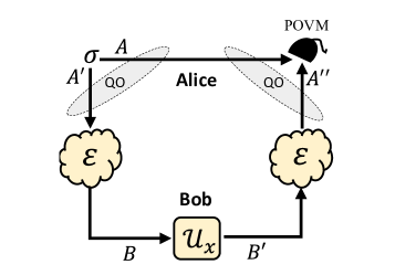
Figure 1: Two-sided noisy dense coding over a quantum channel $\mathcal{E}$. Alice prepares locally the bipartite state $\sigma_{AA^{\prime}}$ and sends system $A^{\prime}$ to Bob who performs the Pauli unitary encoding $\mathcal{U}_{x}$ and sends the system back through the quantum channel. At the ouput Alice performs a joint positive-valued operator measure (POVM) in order to retrieve $x$. In an adaptive version of the protocol, Alice performs quantum operations (QOs) on her input and output systems which are generally updated and optimized round-by-round. These QOs may also be conditioned by an extra assisting variable which is communicated back by Bob.

Dense coding protocol.– Let us recall the expressions of Pauli operators in a $d$-dimensional Hilbert space. On a computational basis $\{|j\rangle\}$, we may define the two shift operators

$$X|j\rangle=|j\oplus 1\rangle,~{}~{}Z|j\rangle=\omega^{j}|j\rangle,$$ (2)

where $\oplus$ is modulo $d$ addition and $\omega:=\exp(2i\pi/d)$. We may then consider the $d^{2}$ Pauli operators $X^{l}Z^{m}$ that, for simplicity, we denote by $U_{x}$ with collapsed index $x=l,m$. For $d=2$, these operators provide the standard qubit Pauli operators $X$, $Y$, $Z$ plus the identity $I$. In the following we use the compact notation $\mathcal{U}_{x}(\rho):=U_{x}\rho U_{x}^{\dagger}$.

Now consider the scheme depicted in Fig. 1 where the communication line between Alice and Bob is affected by a completely positive trace-preserving (CPTP) map $\mathcal{E}$. Alice’s resource state $\sigma_{AA^{\prime}}$ is defined on a $d\times d$-dimensional Hilbert space. Part $A^{\prime}$ is sent to Bob who encodes classical variable $X:=\{x,\pi_{x}\}$ by means of $d^{2}$ Pauli operators $\mathcal{U}_{x}$ which are chosen with probability $\pi_{x}$. In this way, Bob generates the state

$$\sigma_{AB^{\prime}}(x):=[\mathcal{I}_{A}\otimes(\mathcal{U}_{x}\circ\mathcal{E})_{A^{\prime}}](\sigma_{AA^{\prime}}),$$ (3)

where $\mathcal{I}(\rho):=I\mathbb{\rho}I^{\dagger}$ is the identity map. Once system $B^{\prime}$ is sent back through the channel, Alice receives the output system $A^{\prime\prime}$ in the state $\rho_{AA^{\prime\prime}}(x):=(\mathcal{I}_{A}\otimes\mathcal{E}_{x})(\sigma_{AA^{\prime}})$ where we have defined the encoding channel

$$\mathcal{E}_{x}:=\mathcal{E}\circ\mathcal{U}_{x}\circ\mathcal{E}.$$ (4)

In order to retrieve the value of $x$, Alice performs a joint quantum measurement on $A$ and $A^{\prime\prime}$. Asymptotically (i.e., for many repetitions of the protocol), the accessible information of Alice’s output ensemble $\{\pi_{x},\rho_{AA^{\prime\prime}}(x)\}$ is given by the Holevo bound HOLE

$$\chi\left(\{\pi_{x},\rho_{AA^{\prime\prime}}(x)\}\right) =$$ (5)

$$S\left[{\textstyle\sum_{x}}\pi_{x}\rho_{AA^{\prime\prime}}(x)\right]-{\textstyle\sum_{x}}\pi_{x}S[\rho_{AA^{\prime\prime}}(x)].$$

The one-shot dense coding capacity (1-DCC) of the channel $C_{D}^{(1)}(\mathcal{E})$ is obtained by optimizing over Bob’s encoding variable and Alice’s input source, i.e., we may write

$$C_{D}^{(1)}(\mathcal{E})=\max_{\sigma,\pi_{x}}\chi\left(\{\pi_{x},\rho_{AA^{\prime\prime}}(x)\}\right)$$ (6)

Adaptive dense coding.– Consider now dense coding over a quantum channel $\mathcal{E}$ where Alice performs QOs in an adaptive fashion. Alice has a quantum register $\mathbf{a}$ as in Fig. 2. At the beginning Alice performs a QO $Q_{0}$ in order to prepare her initial state $\rho_{\mathbf{a}}^{0}$. She then selects one system $a_{1}^{\prime}\in\mathbf{a}$ and sends it through $\mathcal{E}$. Once Bob receives the output $b_{1}$, he encodes the message $x_{1}$ by means of a Pauli operator $\mathcal{U}_{x_{1}}$ with probability $\pi_{x_{1}}$. This procedure gives rise to the state $\rho_{\mathbf{a}b_{1}^{\prime}}^{0}(x_{1})$. Bob sends the system $b_{1}^{\prime}$ backward to Alice through $\mathcal{E}$. At the output, Alice incorporates the received system $a_{1}^{\prime\prime}$ in her local register which is updated as $\mathbf{a}a_{1}^{\prime\prime}\rightarrow\mathbf{a}$. Next, Alice performs an optimized QO $Q_{1}$ on the register with output state $\rho_{\mathbf{a}}^{1}(x_{1})$. In the second transmission Alice picks another system $a_{2}^{\prime}\in\mathbf{a}$ and she transmits it to Bob who receives $b_{2}$. Bob applies the second Pauli operator $\mathcal{U}_{x_{2}}$ with probability $\pi_{x_{2}|x_{1}}$ and sends the system back to Alice who performs another optimized QO $Q_{2}$ obtaining the state $\rho_{\mathbf{a}}^{2}(x_{1}x_{2})$. After $n$ uses, Alice’s the output state will be $\rho_{\mathbf{a}}^{n}(\mathbf{x}_{n})$ where $\mathbf{x}_{i}=x_{1}x_{2}\ldots x_{i}$ is the encoded message with probability $\pi_{\mathbf{x}_{i}}=\pi_{x_{i}|x_{i-1}\cdots x_{1}}\cdots\pi_{x_{2}|x_{1}}\pi_{x_{1}}$.

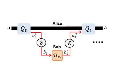
Figure 2: Adaptive dense coding protocol over the quantum channel $\mathcal{E}$. Each encoding and round-trip transmission occurs between two quantum operations (QOs). This is the first use of the protocol. See text for more details.

On average, Alice receives the ensemble $\{\pi_{\mathbf{x}_{n}},\rho_{\mathbf{a}}^{n}(\mathbf{x}_{n})\}$ where the output state $\rho_{\mathbf{a}}^{n}(\mathbf{x}_{n})$ depends on the encoded classical information and the sequence of QOs $\mathcal{Q}:=\{Q_{1},Q_{2},\ldots Q_{n}\}$. Alice’s deferred measurement NiCh will be done on the final state. For large $n$, and optimizing the Holevo information of the ensemble $\mathcal{P}$ over all the possible sequences $\mathcal{Q}$, we define the dense coding capacity (DCC) of the quantum channel $\mathcal{E}$ as

$$C_{D}(\mathcal{E}):=\sup_{\mathcal{Q}}\max_{\pi_{\mathbf{x}_{n}}}\lim_{n}n^{-1}\chi(\{\pi_{\mathbf{x}_{n}},\rho_{\mathbf{a}}^{n}(\mathbf{x}_{n})\})~{}.$$ (7)

Note that this definition is more general than a regularized version $C_{D}^{\infty}(\mathcal{E})$ of Eq. (6), where Alice prepares a large multipartite input state, sends part of this state through $n$ uses of the round-trip and then performal global measurement of the total output. In fact, Eq. (7) assumes that Alice’s input can also be updated round-by-round on the basis of feedback from Bob NotaC .

Single-letter upper bound.– We now exploit a number of ingredients from recent literature to derive a computable upper bound for the DCC. Recall that, for any finite-dimensional quantum channel $\mathcal{E}$, we may write the simulation $\mathcal{E}(\rho)=\mathcal{T}(\rho\otimes\sigma)$, where $\mathcal{T}$ is a trace-preserving LOCC and $\sigma$ a resource state PLOB . Furthermore, suppose that the channel is covariant with respect to Pauli operators so that, for any Pauli $\mathcal{U}$, we may write $\mathcal{E}\circ\mathcal{U}=\mathcal{U}^{\prime}\circ\mathcal{E}$ for some generally-different Pauli $\mathcal{U}^{\prime}$. In this case the channel is Pauli-covariant and we may write RevSim ; PLOB $\mathcal{E}(\rho)=\mathcal{T}_{\text{tele}}(\rho\otimes\sigma_{\mathcal{E}})$, where $\mathcal{T}_{\text{tele}}$ is a teleportation LOCC and $\sigma_{\mathcal{E}}$ is the channel’s Choi matrix, i.e., $\sigma_{\mathcal{E}}:=\mathcal{I}_{A}\otimes\mathcal{E}(\Phi_{AB})$ with $\Phi_{AB}$ being a maximally-entangled state. Note that the Pauli unitaries $\mathcal{U}_{x}$ are jointly Pauli-covariant, i.e., we may certainly write $\mathcal{U}_{x}\circ\mathcal{U}=\mathcal{U}^{\prime}\circ\mathcal{U}_{x}$ where $\mathcal{U}^{\prime}$ is the same for any $x$ (since a Pauli operator either commutes or anti-commutes with another Pauli operator). Therefore, if $\mathcal{E}$ is Pauli-covariant, we also have that the encoding channel $\mathcal{E}_{x}$ is jointly Pauli-covariant. We may therefore write the channel simulation $\mathcal{E}_{x}(\rho)=\mathcal{T}_{\text{tele}}(\rho\otimes\sigma_{\mathcal{E}_{x}})$ in terms of its Choi matrix.

$$\sigma_{\mathcal{E}_{x}}:=\mathcal{I}_{A}\otimes\mathcal{E}_{x}(\Phi_{AB}).$$ (8)

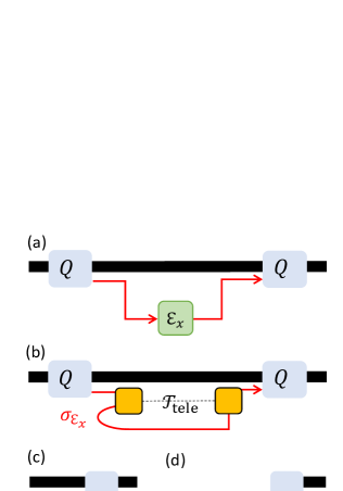
Figure 3: Stretching of adaptive dense coding. (a) Replace the round-trip process of Fig. 2 with a total $x$-depending channel $\mathcal{E}_{x}$. (b) Simulate $\mathcal{E}_{x}$ by teleporting $\mathcal{T}_{\text{tele}}$ over the Choi matrix $\sigma_{\mathcal{E}_{x}}$. (c) Collapse the QOs and the LOCC $\mathcal{T}_{\text{tele}}$ into a single QO $\Delta$. (d) Repeat for all the $n$ uses, so as to collect an ensemble of Choi matrices subject to a global QO $\Lambda$.

The next step is the stretching of the protocol as explain in Fig. 3. Thanks to this procedure the output state can be decomposed in a tensor product of Choi matrices up to a global QO $\Lambda$, i.e., we may write

$$\rho_{\mathbf{a}}^{n}(\mathbf{x}_{n})=\Lambda(\sigma_{\mathcal{E}_{x_{1}}}^{\otimes n_{x_{1}}}\otimes\sigma_{\mathcal{E}_{x_{2}}}^{\otimes n_{x_{2}}}\otimes\ldots\otimes\sigma_{\mathcal{E}_{x_{n}}}^{\otimes n_{x_{n}}})~{},$$ (9)

where the $n_{x_{i}}$ is the number of $x_{i}$ occurrences in the message $\mathbf{x}_{n}$. This given by $n_{x_{i}}=n\pi_{x_{i}}$ where $\pi_{x_{i}}=\sum_{j\neq i}\pi_{\mathbf{x}_{n}}$ is the marginal probability. Thanks to Eq. (9) we can simplify the Holevo quantity in Eq. (7). In fact, by using ($\star$) the contractivity under CPTP maps of the Holevo quantity, and ($\bullet$) the subadditivity of the Von Neumann entropy $S$ under tensor products, we may write

$$\chi(\{\pi_{\mathbf{x}_{n}},\rho_{\mathbf{a}}^{n}(\mathbf{x}_{n})\})\overset{(\star)}{\leq}\chi\left(\left\{\pi_{\mathbf{x}_{n}},{\textstyle\bigotimes_{i=1}^{n}}\sigma_{\mathcal{E}_{x_{i}}}^{\otimes n_{x_{i}}}\right\}\right)$$

$$=S\left({\textstyle\sum_{\mathbf{x}_{n}}}\pi_{\mathbf{x}_{n}}{\textstyle\bigotimes_{i}}\sigma_{\mathcal{E}_{x_{i}}}^{\otimes n_{x_{i}}}\right)-{\textstyle\sum_{\mathbf{x}_{n}}}\pi_{\mathbf{x}_{n}}S\left({\textstyle\bigotimes_{i}}\sigma_{\mathcal{E}_{x_{i}}}^{\otimes n_{x_{i}}}\right)$$

$$\overset{(\bullet)}{\leq}n_{x_{1}}S({\textstyle\sum_{\mathbf{x}_{n}}}\pi_{\mathbf{x}_{n}}\sigma_{\mathcal{E}_{x_{1}}})+\ldots+n_{x_{n}}S({\textstyle\sum_{\mathbf{x}_{n}}}\pi_{\mathbf{x}_{n}}\sigma_{\mathcal{E}_{x_{n}}})$$

$$-n_{x_{1}}{\textstyle\sum_{\mathbf{x}_{n}}}\pi_{\mathbf{x}_{n}}S\left(\sigma_{\mathcal{E}_{x_{1}}}\right)-\ldots-n_{x_{n}}{\textstyle\sum_{\mathbf{x}_{n}}}\pi_{\mathbf{x}_{n}}S\left(\sigma_{\mathcal{E}_{x_{n}}}\right)$$

$$\leq nS\left({\textstyle\sum_{x}}\pi_{x}\sigma_{\mathcal{E}_{x}}\right)-n{\textstyle\sum_{x}}\pi_{x}S\left(\sigma_{\mathcal{E}_{x}}\right)$$

$$=n\chi(\{\pi_{x},\sigma_{\mathcal{E}_{x}}\}),$$ (10)

where $\pi_{x}$ is the marginal probability of a generic letter $x$ and the Choi matrix $\sigma_{\mathcal{E}_{x}}$ is defined in Eq. (8). Note that, in the last inequality of Eq. (10), we also use the fact that a random code NiCh ; Shan , i.e., a code where the codewords are randomly chosen with an iid distribution equal to the marginal probability $\pi_{x}$, is known to achieve the Holevo bound for discrete memoryless quantum channels HSW1 ; HSW2 .

By using Eq. (10) in the definition of Eq. (7), we may then get rid of the supremum over $\mathcal{Q}$ and the asymptotic limit in $n$. We may therefore write a single-letter upper bound for the DCC of a Pauli-covariant channel $\mathcal{E}$ as

$$C_{D}(\mathcal{E})\leq\max_{\pi_{x}}\chi(\{\pi_{x},\sigma_{\mathcal{E}_{x}}\})~{},$$ (11)

where $\pi_{x}$ is the marginal probability distribution of Bob’s encoding variable, and $\sigma_{\mathcal{E}_{x}}$ is the Choi matrix of the encoding channel $\mathcal{E}_{x}$ in Eq. (4). Note that the upper bound in Eq. (11) may be reached asymptotically by a non-adaptive protocol where Alice prepares maximally-entangled states $\Phi_{AA^{\prime}}$ and sends $A^{\prime}$ through the channel, while Bob applies independent Pauli operators $\mathcal{U}_{x}$ with optimized probability $\pi_{x}$. Therefore, for a Pauli-covariant channel we conclude that

$$C_{D}(\mathcal{E})=C_{D}^{(1)}(\mathcal{E})=\max_{\pi_{x}}\chi(\{\pi_{x},\sigma_{\mathcal{E}_{x}}\}).$$ (12)

Remarkably, no adaptiveness or regularization is needed to achieve the best possible dense coding performance with a Pauli-covariant channel.

Dense coding capacity of Pauli channels.– The main result in Eq. (12) can be applied to any Pauli channel at any finite dimension $d.$ For any $d\geq 2$, a Pauli channel takes the form

$$\mathcal{E}^{d}(\rho)=\sum_{k,r=0}^{d-1}p_{kr}\left(X^{k}Z^{r}\right)\rho\left(X^{k}Z^{r}\right)^{\dagger},$$ (13)

where $p_{kr}$ is a probability distribution, and $X$ and $Z$ are the $d$-dimensional shift operators in Eq. (2). For this channel, we may easily write an explicit formula for its DCC capacity. In evaluating the Holevo bound, we notice that von Neumann entropy $S\left({\textstyle\sum_{x}}\pi_{x}\sigma_{\mathcal{E}_{x}^{d}}\right)$ is maximized by the uniform probability $\pi_{x}=1/d^{2}$ and we can write $S\left({\textstyle\sum_{x}}\pi_{x}\sigma_{\mathcal{E}_{x}^{d}}\right)=\log_{2}d^{2}$. Then, using the invariance of the entropy under unitary transformations, one has ${\textstyle\sum_{x}}\pi_{x}S(\sigma_{\mathcal{E}_{x}^{d}})=S\left[\mathcal{I}_{A}\otimes\mathcal{E}^{d}(\sigma_{\mathcal{E}^{d}})\right]$. Therefore, for the Holevo quantity in Eq. (12) we may write

$$C_{D}(\mathcal{E}^{d})=\log d^{2}-S\left[\mathcal{I}_{A}\otimes\mathcal{E}^{d}(\sigma_{\mathcal{E}^{d}})\right].$$ (14)

As expected this is strictly less than the entanglement-assisted classical capacity of the channel, given by CEA1 ; CEA2

$$C_{E}(\mathcal{E})=\log d^{2}-S(\sigma_{\mathcal{E}^{d}})~{}.$$ (15)

Consider a qubit depolazing channel, which is a Pauli channel of the form

$$\mathcal{E}_{\text{depol}}^{2}(\rho)=\left(1-\frac{3}{4}p\right)\rho+\frac{p}{4}(X\rho X+Y\rho Y+Z\rho Z),$$ (16)

for some probability $p$. Then, it is straighforward to see that $C_{D}(\mathcal{E}_{\text{depol}}^{2})=2-h_{2}\left(\alpha\right)-\alpha\log 3$, where $h_{2}(x)=-x\log x-(1-x)\log(1-x)$ is the binary entropy function and $\alpha:=3/4p(2-p)$. Then, consider a qubit dephasing channel, which takes the form

$$\mathcal{E}_{\text{deph}}^{2}(\rho)=(1-p)\rho+pZ\rho Z~{}.$$ (17)

Its DCC is equal to the following expression

$$C_{D}(\mathcal{E}_{\text{deph}}^{2})=2[1-h_{2}(p)],$$ (18)

for $p\leq 1/2$ and zero otherwise.

Conclusion.– In this work we have considered the most general adaptive protocol for the dense coding of classical information in a realistic scenario where noise affects both the communication lines between Alice and Bob. Assuming that this noise is modelled by the same quantum channel, we define its dense coding capacity as the maximum amount of classical information (per round-trip use) that Bob can transmit to Alice. We assume that Bob is implementing Pauli encoders with an optimized probability distribution and Alice is using quantum registers that are adaptively updated and optimized in the process. For Pauli-covariant channel, we find that this capacity reduces to a single-letter version based on a protocol which is non-adaptive and one-shot (i.e., using iid input states). In particular, we can establish exact formulas for the dense coding capacity of Pauli channels.

Note that our approach departs from the definition of entanglement-assisted classical capacity of a quantum channel CEA1 ; CEA2 , where it is implicitly required that the parties either have a noiseless side quantum channel for distributing entangled sources or they have previously met and stored quantum entanglement in ideal long-life quantum memories. Our treatment and definition of dense coding capacity removes these assumptions assuming that the entanglement source is itself distributed through the noisy channel and, therefore, it is realistically degraded by the environment. Because of this feature, our capacity can also be seen as an upper bound for the key rates of two-way quantum key distribution protocols that are related to the dense coding idea pp1 ; pp2 ; pp3 ; pp4 ; pp5 .

Acknowledgments.– This work was supported by the EPSRC via the ‘UK Quantum Communications Hub’ (EP/M013472/1) and the EC via “Continuous Variable Quantum Communications” (CiViQ, 820466).

References

- (1) M. A. Nielsen, and I. L. Chuang, Quantum computation and quantum information (Cambridge University Press, Cambridge, 2000).
- (2) J. Watrous, The theory of quantum information (Cambridge University Press, Cambridge, 2018).
- (3) A. Holevo, Quantum Systems, Channels, Information: A Mathematical Introduction (De Gruyter, Berlin-Boston, 2012).
- (4) C. Weedbrook et al., Rev. Mod. Phys. 84, 621 (2012).
- (5) C. H. Bennett, G. Brassard, C. Crepeau, R. Jozsa, A. Peres, and W. K. Wootters, Phys. Rev. Lett. 70, 1895 (1993).
- (6) S. Pirandola et al., Nature Photon. 9, 641-652 (2015).
- (7) C. H. Bennett, and G. Brassard. Proc. of IEEE International Conference on Computers, Systems and Signal Processing 175, 8. New York, 1984.
- (8) C. H. Bennett and S. J. Wiesner, Phys. Rev. Lett. 69, 2881 (1992).
- (9) T. Hiroshima, J. Phys. A 34, 6907 (2001).
- (10) M. Ziman and V. Bužek, Phys. Rev. A 67, 042321 (2003).
- (11) It is clear that entangled states with positive partial transpose, i.e. bound entangled states, are not useful for dense coding, since for these states we have so that they cannot be exploited to transmit at a rate greater than .
- (12) C. H. Bennett, P. W. Shor, J. A. Smolin and A. V. Thapliyal, Phys. Rev. Lett. 83, 3081 (1999)
- (13) C. H. Bennett, P. W. Shor, J. A. Smolin and A. V. Thapliyal, IEEE Trans. Inf. Theory 48, 2637–2655 (2002).
- (14) Z. Shadman, H. Kampermann, C. Macchiavello, and D. Bruß, New J. Phys. 12, 073042 (2010).
- (15) Z. Shadman, H. Kampermann, D. Bruß, and C. Macchiavello, Phys. Rev. A 84, 042309 (2011).
- (16) Z. Shadman, H.Kampermann, C. Macchiavello, D. Bruß, Quantum Meas. Quantum Metrol. 1, 21–33 (2013).
- (17) S. Pirandola, R. Laurenza, C. Ottaviani, and L. Banchi, Nat. Commun. 8, 15043 (2017).
- (18) S. Pirandola, B. Roy Bardhan, T. Gehring, C. Weedbrook, and S. Lloyd, Nat. Photon. 12, 724–733 (2018).
- (19) S. Pirandola, S. L. Braunstein, R. Laurenza, C. Ottaviani, and L. Banchi, Quant. Sci. Tech. 3, 035009 (2018).
- (20) R. Laurenza, C. Lupo, G. Spedalieri, S. L. Braunstein, and S. Pirandola, Quantum Meas. Quantum Metrol. 5, 1–12 (2018).
- (21) A. S. Holevo, Prob. Inf. Transm. 9, 177–183 (1973).
- (22) Note that one might consider a generalized dense coding protocol, where Bob uses arbitrary encoding unitaries instead of Pauli operators. Correspondingly, we may introduce a generalized dense coding capacity as in Eq. (7) but replacing the maximization as , where are sequences of arbitrary unitary encoders. By definition, we have . However we conjecture that an equality should hold, due to the fact that the basis of Pauli operators represents the optimal choice in the noise-less scenario.
- (23) C. E. Shannon, “A mathematical theory of Communication,” The Bell System Technical Journal 27, 379–423 and 623–656 (1948).
- (24) A. S. Holevo, IEEE Trans. Inf. Theory 44, 269–273 (1998).
- (25) B. Schumacher, and M. Westmoreland, Phys. Rev. A 56, 131–138 (1997).
- (26) K. Bostrom and T. Felbinger, Phys. Rev. Lett. 89, 187902 (2002).
- (27) Q.-Y. Cai, Phys. Rev. Lett. 91, 109801 (2003).
- (28) F.-G. Deng and G. L. Long, Phys. Rev. A 69, 052319 (2004).
- (29) Q.-Y. Cai and B.-W. Li, Chin. Phys. Lett. 21, 601 (2004).
- (30) M. Lucamarini and S. Mancini, Phys. Rev. Lett. 94, 140501 (2005).