The ALMA Spectroscopic Survey in the HUDF: Nature and physical properties of gas-mass selected galaxies using MUSE spectroscopy

Abstract

We discuss the nature and physical properties of gas-mass selected galaxies in the ALMA spectroscopic survey (ASPECS) of the Hubble Ultra Deep Field (HUDF). We capitalize on the deep optical integral-field spectroscopy from the MUSE HUDF Survey and multi-wavelength data to uniquely associate all 16 line-emitters, detected in the ALMA data without preselection, with rotational transitions of carbon monoxide (CO). We identify ten as CO(2-1) at $1<z<2$, five as CO(3-2) at $2<z<3$ and one as CO(4-3) at $z=3.6$. Using the MUSE data as a prior, we identify two additional CO(2-1)-emitters, increasing the total sample size to 18. We infer metallicities consistent with (super-)solar for the CO-detected galaxies at $z\leq 1.5$, motivating our choice of a Galactic conversion factor between CO luminosity and molecular gas mass for these galaxies. Using deep Chandra imaging of the HUDF, we determine an X-ray AGN fraction of 20% and 60% among the CO-emitters at $z\sim 1.4$ and $z\sim 2.6$, respectively. Being a CO-flux limited survey, ASPECS-LP detects molecular gas in galaxies on, above and below the main sequence (MS) at $z\sim 1.4$. For stellar masses $\geq 10^{10}(10^{10.5})$ $\mathrm{M}_{\odot}$, we detect about 40% (50%) of all galaxies in the HUDF at $1<z<2$ ($2<z<3$). The combination of ALMA and MUSE integral-field spectroscopy thus enables an unprecedented view on MS galaxies during the peak of galaxy formation.

1 Introduction

Star formation takes place in the cold interstellar medium (ISM) and studying the cold molecular gas content of galaxies is therefore fundamental for our understanding of the formation and evolution of galaxies. As there is little to no emission from the molecular hydrogen that constitutes the majority of the molecular gas in mass, cold molecular gas is typically traced by molecules, such as the bright rotational transitions of ¹²C¹⁶O (hereafter CO).

Recent years have seen a tremendous advance in the characterization of the molecular gas content of high redshift galaxies (for a review, see Carilli & Walter, 2013). Targeted surveys with the Atacama Large Millimetre Array (ALMA) and the Plateau de Bure Interferometer (PdBI) have been instrumental in our understanding of the increasing molecular gas reservoirs of star-forming galaxies at $z>1$ (Daddi et al., 2010, 2015; Genzel et al., 2010; Tacconi et al., 2010, 2013; Silverman et al., 2015, 2018). Combining data across cosmic time, these provide constraints on how the molecular gas content of galaxies evolves as a function of their physical properties, such as stellar mass ($M_{*}$) and star formation rate (SFR) (Scoville et al., 2014, 2017; Genzel et al., 2015; Saintonge et al., 2016; Tacconi et al., 2013, 2018). These surveys typically target galaxies with SFRs that are greater than or equal to the majority of the galaxy population at their respective redshifts and stellar masses (the ‘main sequence’ of star-forming galaxies; Brinchmann et al. 2004; Noeske et al. 2007; Whitaker et al. 2014; Schreiber et al. 2015; Eales et al. 2018; Boogaard et al. 2018), and therefore should be complemented by studies that do not rely on such a preselection.

Spectral line scans in the (sub-)millimeter regime in deep fields provide a unique window on the molecular gas content of the universe. As the cosmic volume probed is well defined, they play a fundamental role in determining the evolution of the cosmic molecular gas density through cosmic time. Through their spectral scan strategy, these surveys are designed to detect molecular gas in galaxies without any preselection, providing a flux-limited view on the molecular gas emission at different redshifts (Walter et al., 2014; Decarli et al., 2014; Walter et al., 2016; Decarli et al., 2016; Riechers et al., 2019; Pavesi et al., 2018). By conducting ‘spectroscopy-of-everything’, these can in principle reveal the molecular gas content in galaxies that would not be selected in traditional studies (e.g., galaxies with a low SFR, well below the main sequence, but a substantial gas mass.).

This paper is part of series of papers presenting the first results from the ALMA Spectroscopic Survey Large Program (ASPECS-LP; Decarli et al. 2019). The ASPECS-LP is a spectral line scan targeting the Hubble Ultra Deep Field (HUDF). Here we use the results from the spectral scan of Band 3 (84-115 GHz; 3.6-2.6 mm) and investigate the nature and physical properties of galaxies detected in molecular emission lines by ALMA. In order to do so, it is important to know about the physical conditions of the galaxies detected in molecular gas, such as their ISM conditions, their (HST) morphology and stellar and ionized gas dynamics. The HUDF benefits from the deepest and most extensive multi-wavelength data, and as of recently, ultra-deep integral-field spectroscopy.

A critical step in identifying ALMA emission lines with actual galaxies relies on matching the galaxies in redshift. In this context, the Multi Unit Spectroscopic Explorer (MUSE, Bacon et al. 2010) HUDF survey, that provides a deep optical integral-field spectroscopic survey over the HUDF (Bacon et al., 2017), is essential. The MUSE HUDF is a natural complement to the ASPECS-LP in the same area on the sky, providing optical spectroscopy for all galaxies within the field of view, also without any preselection. In addition, the integral-field spectrograph provides redshifts for over a thousands of galaxies in the HUDF (increasing the number of previously known redshifts by a factor $\sim 10\times$; Inami et al. 2017). Depending on the redshift, these data can provide key information on the ISM conditions (such as metallicity and dynamics) of the galaxies harboring molecular gas. As we will see throughout this paper, the MUSE data are a significant step forward in our understanding of galaxy population selected with ALMA.

The paper is organized as follows: We first introduce the spectroscopic and multi-wavelength data (§ 2). We discuss the redshift identification of the CO-detected galaxies from the line search (Gonzalez-Lopez et al., 2019), using the MUSE and multi-wavelength data, in § 3.1. Next, we leverage the large number of MUSE redshifts to separate real from spurious sources down to a significantly lower signal-to-noise ratios (S/N) than possible in the line search (§ 3.2). Together, these sources form the full ASPECS-LP Band 3 sample (§ 3.3). We then move on to the central question(s) of this paper: By doing a survey of molecular gas, in what kind of galaxies do we detect molecular gas emission at different redshifts, and what are the physical properties of these galaxies? We determine stellar masses, SFRs and (where possible) metallicities for all sources in (§ 4) and link these to the molecular gas content ($M_{\mathrm{mol}}$) to derive the gas fraction ($M_{\mathrm{mol}}/M_{*}$, the molecular-to-stellar mass ratio) and depletion time ($t_{\mathrm{depl}}=M_{\mathrm{mol}}/\mathrm{SFR}$). We first discuss the properties of the sample of CO-detected galaxies in the context of the overall population of the HUDF (§ 5.1) and investigate the X-ray AGN fraction among the detected sources (§ 5.2). Using the MUSE spectra, we determine the unobscured SFR (§ 5.3) and the metallicity of the $1<z<1.5$ sources (§ 5.4). Finally, we discuss the CO detected galaxies from the flux-limited survey in the context of the galaxy main sequence (§ 6), focusing on the molecular gas mass, gas fraction and depletion time. We discuss what fraction of the galaxy population in the HUDF we detect with increasing redshift. A further discussion of the molecular gas properties of these sources data will be presented in Aravena et al. (2019).

Throughout this paper, we adopt a Chabrier (2003) IMF and a flat $\Lambda$CDM cosmology, with $H_{0}=70$ km s^-1 Mpc^-1, $\Omega_{m}=0.3$ and $\Omega_{\Lambda}=0.7$. Magnitudes are in the AB system (Oke & Gunn, 1983).

2 Observations

2.1 ALMA Spectroscopic Survey

We focus on the ASPECS-LP Band 3 observations, that have been completed in ALMA Cycle 4. The acquisition and reduction of the Band 3 data are described in detail in Decarli et al. (2019). The final mosaic covers a 4.6 arcmin² area in the HUDF (where the primary beam response is $>50\%$ of the peak sensitivity). The data are combined into a single spectral cube with a spatial resolution of $\approx 1.75\arcsec\times 1.49\arcsec$ (synthesized beam with natural weighting at 99.5 GHz) and a spectral resolution of 7.813 MHz, corresponding to $\Delta v\approx 23.5$ km s^-1 at 99.5 GHz. The average root mean square (rms) sensitivity is $\approx 0.2$ mJy beam^-1 but varies across the frequency range, being deepest ($\approx 0.13$ mJy beam^-1) around 100 GHz and higher above 110 GHz, due to the spectral setup of the observations (see Gonzalez-Lopez et al. 2019 for details). Throughout this paper, we consider the area that lies within $>40\%$ of the primary beam peak sensitivity, which is the shallowest part of the survey over which we still detect CO candidates without preselection (§ 3.1). When comparing to the HST reference frame, we take into account an astrometric offset of $\Delta\alpha=+0.076\arcsec,\Delta\delta=-0.279\arcsec$ (Dunlop et al., 2017; Rujopakarn et al., 2016).

We perform an extensive search of the cube for molecular emission lines, as is detailed in Gonzalez-Lopez et al. (2019) and § 3. With the Band 3 data alone, the ASPECS-LP is sensitive to different CO and $\mathrm{[C\,\textsc{i}]}$ transitions at specific redshift ranges which are indicated in the top panel of Fig. 1.

2.2 MUSE HUDF Survey

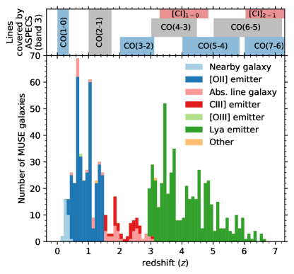
Figure 1: The molecular line redshift coverage of the galaxies in the MUSE and ASPECS-LP Hubble Ultra Deep Field (HUDF). The histogram shows the galaxies with spectroscopic redshifts from MUSE (udf10 and mosaic; see § 2.2) that lie within $>40\%$ of the primary beam sensitivity of the ASPECS-LP mosaic, distinguished by the primary spectral feature used to identify the redshift (Inami et al. 2017; ‘Nearby galaxy’ summarizes a range of rest-frame optical features). The decrease in the number of redshifts between $1.5<z<2.9$ is due to the lack of strong emission line features in the MUSE spectrograph (‘redshift desert’). The drop at the lowest redshifts is due to the nature and volume of the HUDF. The top panel shows the specific CO and $\mathrm{[C\,\textsc{i}]}$ transitions covered by the frequency setup of ASPECS Band 3 at different redshifts (Walter et al., 2016; Decarli et al., 2019). ASPECS covers CO(2-1) for $\mathrm{[O\,\textsc{ii}]}$ emitters and absorption line galaxies at $1.0<z<1.74$. Galaxies with CO(3-2) at $2.0<z<3.11$ are identified mostly by UV absorption and weaker emission lines (e.g., $\mathrm{C\,\textsc{iii}]}$). For higher-order CO and $\mathrm{[C\,\textsc{i}]}$ transitions above $z>2.90$, MUSE has coverage of $\mathrm{Ly}\alpha$.

The HUDF was observed with the MUSE as part of the MUSE Hubble Ultra Deep Field survey (Bacon et al., 2017). The location on the sky of the ASPECS-LP with respect to the MUSE HUDF is shown in Decarli et al. (2019), Fig. 1. The MUSE integral-field spectrograph has a $1^{\prime}\times 1^{\prime}$ field-of-view, covering the optical regime ($4750-9300$Å) at an average spectral resolution of $\lambda/\Delta\lambda\approx 3000$. The HUDF was observed in a two tier strategy, with the mosaic-region reaching a median depth of 10 hours in a $3^{\prime}\times 3^{\prime}$-region and the udf10-pointing reaching 31 hours depth in a $1^{\prime}\times 1^{\prime}$-region (3$\sigma$ emission line depth for a point source of 3.1 and 1.5 $\times 10^{-19}$ erg s^-1 cm^-2 at 7000Å, respectively). The data acquisition and reduction as well as the automated source detection are described in detail in Bacon et al. (2017). The measured seeing in the reduced datacube is $0\farcs 65$ full-width at half-maximum (FWHM) at 7000Å.

Redshifts were identified semi-automatically and the full spectroscopic catalog is presented in Inami et al. (2017). The spectra were extracted using a weighted extraction, where the weighting was based on the MUSE white light image, to obtain the maximal signal-to-noise. The spectra are modeled with a modified version of platefit (Tremonti et al., 2004; Brinchmann et al., 2004, 2008) to obtain line-flux measurements and equivalent widths for all sources. The typical uncertainty on the redshift measurement is $\sigma_{v}=0.00012(1+z)$ or $\approx 40$ km s^-1 (Inami et al., 2017), which we use to compute the uncertainties in the relative velocities.

In order to compare in detail the relative velocities measured between the UV/optical features in MUSE and CO in ALMA, we need to place both on the same reference frame. The MUSE redshifts are provided in the barycentric reference frame, while the ALMA cube is set to the kinematic local standard of rest (LSRK). When determining detailed velocity offsets we place both on the same reference frame by removing the velocity difference; $\mathrm{BARY}-\mathrm{LSRK}=-16.7$ km s^-1 (accounting for the angle between the LSRK vector and the observation direction towards the HUDF).

The redshift distribution of the MUSE galaxies that fall within $>40\%$ of the primary beam peak sensitivity of the ASPECS-LP footprint in the HUDF is shown in Fig. 1, where galaxies are color coded by the primary spectral feature(s) used to identify the redshift (see Inami et al. 2017 for details). The redshifts that correspond to the ASPECS band 3 coverage of the different molecular lines are indicated in the top panel. CO(1-0) [115.27 GHz] is observable at the lowest redshifts ($z<0.3694$), where MUSE still covers a major part of the rest-frame optical spectrum that contains a wealth of spectral features, including absorption and (strong) emission lines (e.g., $\mathrm{H}\alpha\ \lambda 6563$, $\mathrm{[O\,\textsc{iii}]}\ \lambda 4959,5007$ and $\mathrm{[O\,\textsc{ii}]}\ \lambda 3726,3729$). The strong lines are the main spectral features used to identify star-forming galaxies all the way up to $z<1.50$, where $\mathrm{[O\,\textsc{ii}]}\ \lambda 3726,3729$ moves out of the spectral range of MUSE. CO(2-1) [230.54 GHz] is covered by ASPECS at $1.0059<z<1.7387$, mostly overlapping with $\mathrm{[O\,\textsc{ii}]}$ in MUSE. At $z>1.5$, the main features used to identify these galaxies are absorption lines such $\mathrm{Mg\,\textsc{ii}}\ \lambda 2796,2803$ and $\mathrm{Fe\,\textsc{ii}\ \lambda 2586,2600}$. Over the redshift range of CO(3-2) [345.80 GHz], $2.0088<z<3.1080$, MUSE only has coverage of weaker UV emission lines (mainly $\mathrm{C\,\textsc{iii}]}\ \lambda 1907,1909$), making redshift identifications more challenging (the ‘redshift desert’). Here, UV absorption lines are commonly used to identify redshifts, for galaxies where the continuum is strong enough ($m_{\mathrm{F775W}}\lesssim 26$ mag). Above $z=2.9$, MUSE flourishes again, with the coverage of $\mathrm{Ly}\alpha\ \lambda 1216$ all the way out to $z\approx 6.7$. Here, ASPECS covers CO(4-3) [461.04 GHz] and transitions with $J_{\rm up}\geq 4$, and atomic carbon lines ($\mathrm{[C\,\textsc{i}]}_{1-0}$ 610 µm and $\mathrm{[C\,\textsc{i}]}_{2-1}$ 370 µm).

2.3 Multi-wavelength data (UV–radio) and Magphys

In order to construct spectral energy distributions (SEDs) for the ASPECS-LP sources, we utilize the wealth of available photometric data over the HUDF, summarized below.

We use the photometric compilation by Skelton et al. (2014, see references therein), which includes UV, optical and near-IR photometry from the Hubble Space Telescope (HST) and ground-based facilities, as well as (deblended) Spitzer/IRAC 3.6µm, 4.5µm, 5.8µm and 8.0µm. We also include the corresponding deblended Spitzer/MIPS 24µm photometry from (Whitaker et al., 2014). We take deblended far-infrared (FIR) data from Herschel/PACS 100µm and 160µm from Elbaz et al. (2011), which have a native resolution of 6$\farcs$7 and 11$\farcs$0, respectively. The PACS 100µm and 160µm have a $3\sigma$ depth of 0.8 mJy and 2.4 mJy and are limited by confusion. For the flux uncertainties we use the maximum of the local and simulated noise levels for each source, as recommended by the documentation. We further include the 1.2 mm continuum data from the combination of the available ASPECS-LP data with the ALMA observations by Dunlop et al. (2017), taken over the same region, as detailed in Aravena et al. (2019). We also include the ASPECS-LP 3.0 mm continuum data, as presented in (Gonzalez-Lopez et al., 2019). For the ASPECS survey we have created a master photometry catalog for the galaxies in the HUDF, adopting the spectroscopic redshifts from MUSE (§ 2.2) and literature sources, as detailed in Decarli et al. (2019).

We use the high-$z$ extension of the SED-fitting code magphys to infer physical parameters from the photometric information of the galaxies in our field (Da Cunha et al., 2008, 2015). The high-$z$ extension of magphys includes a larger library of spectral emission models that extend to higher dust optical depths, higher SFRs and younger ages compared to what is typically found in the local universe. From the spectral emission models, the code can constrain the stellar mass, sSFR and the dust attenuation ($A_{V}$) along the line of sight. An energy balance argument ensures that the amount of absorption at rest-frame UV/optical wavelengths is consistent with the light reradiated in the infrared. The code performs a Bayesian inference of the posterior likelihood distribution of the fitted parameter, to account for uncertainties such as degeneracies in the models, missing data and non-detections.

We run magphys on all the galaxies in our catalog, using the available photometric information in all the bands (listed in Appendix B). We do not include the Spitzer/MIPS and Herschel/PACS photometry in the fits of the general sample because the angular resolution of these observations is relatively modest ($>5\arcsec$), thus a delicate de-blending analysis would be required (the average sky density of galaxies in the HUDF is $\gtrsim$ 1 galaxy per 3 arcsec²). For the CO-detected galaxies we repeat the magphys fits including these bands (§ 4.1). In order to take into account systematic errors in the zero point fitting for these sources, we add the zero point errors (Skelton et al., 2014) in quadrature to the flux errors in all filters except HST, and include a 5% error-floor to further account for systematic errors in the physical models (following Leja et al. 2018). The filter selection of the general sample provides excellent photometric coverage of the stellar population. Paired with the wealth of spectroscopic redshifts (see Decarli et al. 2019 for a detailed description), this enables robust constraints on properties such as $M_{*}$, SFR and $A_{V}$. We do note that while the formal uncertainties on the inferred properties are generally small, systematic uncertainties can be of order $\sim 0.3$ dex (e.g., Conroy, 2013).

2.4 X-ray photometry

To identify AGN in the field, we use the Chandra X-ray data available over the GOODS-S region from Luo et al. (2017), which reaches the full depth of 7 Ms over the HUDF area. In total, there are 36 X-ray sources within the ASPECS-LP region of the HUDF (i.e., within 40% of the primary beam). We spatially cross-match the X-ray catalog to the closest source within 1″ in our MUSE and multi-wavelength catalog over the ASPECS-LP area, visually inspecting all matches used in this paper to ensure they are accurately identified.

At the depth of the X-ray data, there are multiple physical mechanisms (e.g., AGN and star formation) that may produce the X-ray emission detected at $0.5-7$ keV. Luo et al. (2017) adopt the following 6 criteria to distinguish X-ray AGN from other sources of X-ray emission, of which at least one needs to be satisfied to be classified as AGN (we refer the reader to Xue et al. 2011, Luo et al. 2017 and references therein for details): (1) $L_{X}\geq 3\times 10^{42}$ erg s^-1, identifying luminous X-ray sources; (2) an effective photon index $\Gamma_{\mathrm{eff}}\leq 1.0$ indicating hard X-ray sources, identifying obscured AGN; (3) X-ray-to-R-band flux ratio of $\log\left(f_{X}/f_{R}\right)>-1$; (4) spectroscopically classified as AGN via, e.g., broad emission lines and/or high excitation lines; (5) X-ray-to-radio flux ratio of $L_{X}/L_{1.4\mathrm{GHz}}\geq 2.4\times 10^{18}$, indicating an excess of X-ray emission over the level expected from pure star formation; (6) X-ray-to-K-band flux ratio of $\log\left(f_{X}/f_{K_{s}}\right)>-1.2$. Note that even with these criteria it is possible that some X-ray sources host low-luminosity or heavily obscured AGN and are currently misclassified.

Overall, there are six X-ray AGN in the ASPECS-LP volume at $1.0<z<1.7$, all of which have a MUSE redshift (one being a broad-line AGN). In the ASPECS-LP volume at $2.0<z<3.1$, there are seven X-ray AGN, three of which have spectroscopic redshifts from MUSE (including one broad-line AGN), and four with a photometric redshift (we discard one source in the catalog with a photometric redshift in this regime for which we cannot securely identify a counterpart in HST). There is one X-ray AGN at a higher redshift, which is also identified by MUSE as a broad-line AGN at $z=3.188$.

3 The ASPECS-LP sample

3.1 Identification of the line search sample

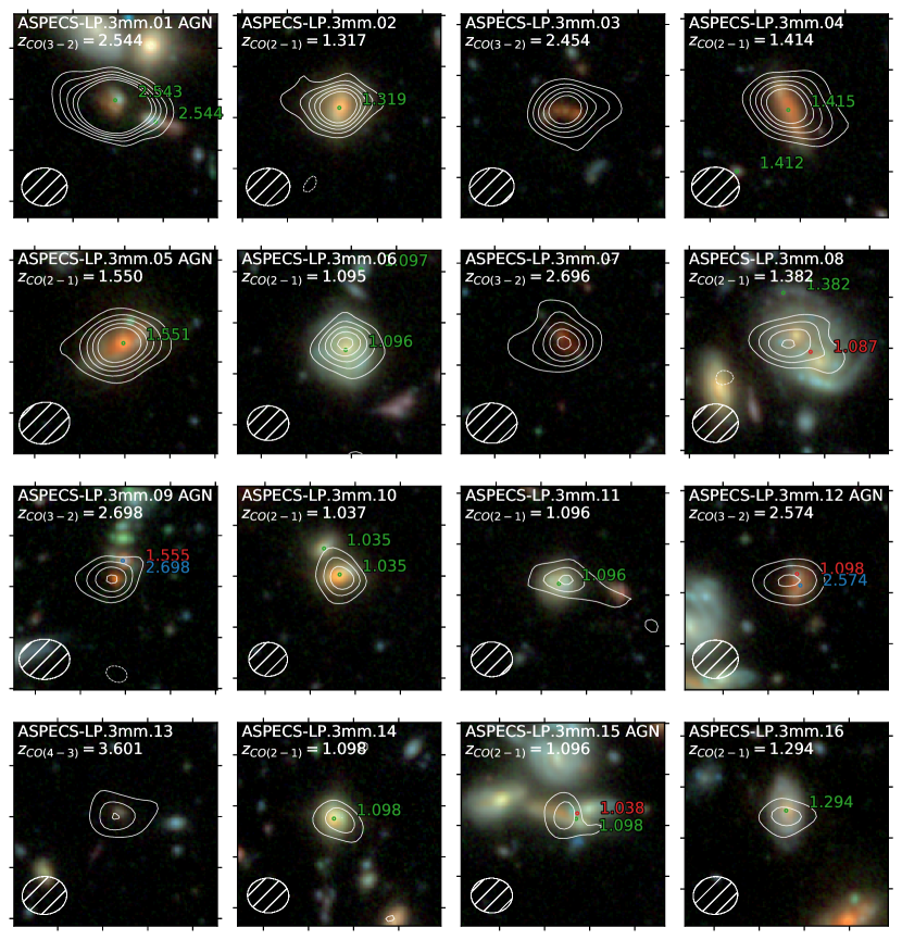
Figure 2: HST RGB cutouts (F160W, F125W, F105W) of the 16 CO line detections from the line search, all revealing an optical/NIR counterpart. Each panel is $8\times 8$ arcsec centered around the CO emission (corrected astrometry; § 2.1). The white contours indicate the CO signal from $\pm[3,..,11]\sigma$ in steps of $2\sigma$. The ALMA beam indicated in the bottom left corner. Galaxies with a spectroscopic redshift from MUSE (Inami et al., 2017) matching the CO signal are labeled in green (and red if not matching); spectroscopic redshifts in blue are newly determined in this paper. Of the 16 galaxies, 12 match closely to a redshift from MUSE (including ASPECS-LP.3mm.08, discussed in Appendix A and Decarli et al. 2016). ASPECS-LP.3mm.03, 3mm.07 and 3mm.09 have $m_{\mathrm{F775W}}>27$, which is too faint for a direct absorption line redshift from MUSE (but are independently confirmed). For ASPECS-LP.3mm.09 we do find UV absorption features matching the CO(3-2) in the galaxy slightly to the north. A new absorption line redshift is found for ASPECS-LP.3mm.12 (see Fig. 18). The photometric redshift and absence of lower-$z$ spectral features indicate ASPECS-LP.3mm.13 being at $z=3.601$.

Table 1: ASPECS-LP CO detected sources from the line search, with MUSE spectroscopic counterparts. The CO frequencies are taken from Gonzalez-Lopez et al. (2019, their Table 7). (1) ASPECS-LP 3mm ID. (2)-(3) Coordinates. (4) CO line Frequency. (5) Identified CO transition (§ 3.1). (6) CO redshift. (7) MUSE ID. (8) MUSE redshift. (9) Velocity offset between MUSE and ALMA ($\Delta v=(z_{\rm MUSE}-z_{\rm CO})/(1+z_{\rm CO})$; after converting both to the same reference frame).

ID	R.A.	Dec.	$\nu_{\mathrm{CO}}$	CO trans.	$z_{\mathrm{CO}}$	MUSE ID	$z_{\mathrm{MUSE}}$	$\Delta v$
	(J2000)	(J2000)	(GHz)	($J_{\rm up}\rightarrow J_{\rm low}$)				km s-1
(1)	(2)	(3)	(4)	(5)	(6)	(7)	(8)	(9)
3mm.01	03:32:38.54	-27:46:34.6	$97.584\pm 0.003$	$3\rightarrow 2$	2.5436	35	2.5432	$-15.5\pm 41.0$
3mm.02	03:32:42.38	-27:47:07.9	$99.510\pm 0.005$	$2\rightarrow 1$	1.3167	996	1.3172∗	$73.5\pm 42.7$
3mm.03	03:32:41.02	-27:46:31.5	$100.131\pm 0.005$	$3\rightarrow 2$	2.4534	$\cdots$	$\cdots$	$\cdots$
3mm.04	03:32:34.44	-27:46:59.8	$95.501\pm 0.006$	$2\rightarrow 1$	1.4140	1117	1.4147	$102.9\pm 44.2$
3mm.05	03:32:39.76	-27:46:11.5	$90.393\pm 0.006$	$2\rightarrow 1$	1.5504	1001	1.5509	$71.7\pm 44.7$
3mm.06	03:32:39.90	-27:47:15.1	$110.038\pm 0.005$	$2\rightarrow 1$	1.0951	8	1.0955	$79.2\pm 42.3$
3mm.07	03:32:43.53	-27:46:39.4	$93.558\pm 0.008$	$3\rightarrow 2$	2.6961	$\cdots$	$\cdots$	$\cdots$
3mm.08	03:32:35.58	-27:46:26.1	$96.778\pm 0.002$	$2\rightarrow 1$	1.3821	6415	1.3820	$-0.1\pm 40.5$
3mm.09	03:32:44.03	-27:46:36.0	$93.517\pm 0.003$	$3\rightarrow 2$	2.6977†	$\cdots$	$\cdots$	$\cdots$
3mm.10	03:32:42.98	-27:46:50.4	$113.192\pm 0.009$	$2\rightarrow 1$	1.0367	1011	1.0362∗	$-53.7\pm 46.6$
3mm.11	03:32:39.80	-27:46:53.7	$109.966\pm 0.003$	$2\rightarrow 1$	1.0964	16	1.0965	$19.8\pm 40.8$
3mm.12	03:32:36.21	-27:46:27.7	$96.757\pm 0.004$	$3\rightarrow 2$	2.5739	1124‡	2.5739∗	$16.8\pm 41.9$
3mm.13	03:32:35.56	-27:47:04.3	$100.209\pm 0.006$	$4\rightarrow 3$	3.6008	$\cdots$	$\cdots$	$\cdots$
3mm.14	03:32:34.84	-27:46:40.7	$109.877\pm 0.009$	$2\rightarrow 1$	1.0981	924	1.0981	$15.0\pm 46.9$
3mm.15	03:32:36.48	-27:46:31.9	$109.971\pm 0.005$	$2\rightarrow 1$	1.0964	6870	1.0979	$240.4\pm 42.3$
3mm.16	03:32:39.92	-27:46:07.4	$100.503\pm 0.004$	$2\rightarrow 1$	1.2938	925	1.2942	$66.3\pm 41.7$
Notes. ∗Updated from Inami et al. (2017), see Appendix A.
†Additionally supported by matching absorption found in MUSE#6941, at $z=2.695$, $0\farcs 7$ to the north.
‡Additional redshift for MUSE#1124, which is cataloged as the foreground $\mathrm{[O\,\textsc{ii}]}$-emitter at $z=1.098$ (see Fig. 18).

An extensive description of the line search is provided in Gonzalez-Lopez et al. (2019). In summary, three independent methods were combined to search for CO lines in the ASPECS-LP band 3 data without any preselection; LineSeeker (González-López et al., 2017), FindClump (Decarli et al., 2014; Walter et al., 2016) and MF3D (Pavesi et al., 2018). The fidelity of these line-candidates was estimated from the ratio of the number of lines with a negative and positive flux detected at a given S/N. Lastly, the completeness of the sample was estimated by ingesting simulated emission lines into the real data cube.

In total, there are 16 emission line candidates for which the fidelity is $\geq 0.9$. Statistical analysis shows that this sample is free from false positives (the sum of their fidelities, based on the ALMA data alone, is 15.9; Gonzalez-Lopez et al. 2019). These 16 sources form the primary, line search-sample and are shown in Fig. 2. All these candidates have a $\mathrm{S/N}\geq 6.4$.

For all sources in the primary sample, one or multiple potential counterpart galaxies are visible in the deep HST imaging shown in Fig. 2. In order to confidently identify a single CO emission line, an independent redshift measurement of the potential counterpart measurement is needed. Given the wealth of multi-wavelength photometry in the HUDF, photometric redshifts can often already provide sufficient constraints to discern between different rotation transitions of CO in the case of isolated galaxies at redshifts $z\lesssim 3$. However, complex systems of several galaxies, or projected superpositions of independent galaxies at distinct redshifts, can make redshift assignments more complicated. Fortunately, the integral-field spectroscopy from MUSE is ideally suited to disentangle spectral features belonging to different galaxies, allowing us to confidently assign redshifts to the CO emission lines. The frequency of a CO line can correspond to different rotational transitions, each with a unique associated redshift. With the potential redshift solutions in hand, we systematically identify the CO line candidates from the line search. We provide a summary of the redshift identifications here. A detailed description of the individual sources and their redshift identifications can be found in Appendix A, where we also show the MUSE spectra for all sources (Fig. 13 – 16).

First, we correlate the spatial position and potential redshifts of the CO lines with known spectroscopic redshifts from MUSE (Inami et al., 2017). From the MUSE redshifts alone, we immediately identify most (11/16) of the CO lines with the highest fidelity. The brightest (ASPECS-LP.3mm.01) is a CO(3-2) emitter at $z=2.54$, showing a wealth of UV absorption features. The other 10 galaxies are a diverse sample of CO(2-1) emitters spanning the redshift range over which we are sensitive; $1.01<z<1.74$. They show a variety of spectra at different levels of S/N, covering a range of UV and optical absorption and emission features. Notably, $\mathrm{[O\,\textsc{ii}]}\ \lambda 3726,3729$ is detected in all galaxies where it is covered by MUSE, while $\mathrm{[Ne\,\textsc{iii}]}\ \lambda 3869$ is detected in some of the higher S/N spectra.

Next, we extract MUSE spectra for the remaining five (5/16) sources without a cataloged redshift and investigate their spectra for a redshift solution matching the observed CO line. We discover two new spectroscopic redshifts at $z=2.54$ (ASPECS-LP.3mm.12) and $z=2.69$ (associated with ASPECS-LP.3mm.09) confirming detections of CO(3-2), which were both not included in the catalog of Inami et al. (2017) as their spectra are blended with foreground sources. The former in particular demonstrates the key use of MUSE in disentangling a spatially overlapping system comprised of a foreground $\mathrm{[O\,\textsc{ii}]}$ emitter and a faint background galaxy, which is detected at $\mathrm{S/N}>4$ both via cross-correlation with a $z\approx 2.5$ spectral template and by stacking absorption features (see Fig. 18). For ASPECS-LP.3mm.03 and ASPECS-LP.3mm.07 we leverage the absence of spectral features (e.g., $\mathrm{[O\,\textsc{ii}]}$, $\mathrm{Ly}\alpha$), consistent with their faint magnitudes ($m_{\mathrm{F775W}}>27$ mag) and a redshift in the MUSE redshift desert, in combination with photometric redshifts in the $z=2-3$ regime from the deep multi-wavelength data, to confirm detections of CO(3-2). Lastly, we find ASPECS-LP.3mm.13 being CO(4-3) at $z=3.601$, based on the photometric redshifts suggesting $z\approx 3.5$ and the absence of a lower redshift solution from the spectrum. $\mathrm{Ly}\alpha\ \lambda 1216$ is not detected for this source, but we caution that at this redshift $\mathrm{Ly}\alpha$ falls very close to the $\mathrm{[O\,\textsc{i}]}\ \lambda 5577$ skyline. Furthermore, given that the source potentially contains significant amounts of dust, no $\mathrm{Ly}\alpha$ emission may be expected at all.

In summary, we determine a redshift solution for all (16/16) candidates from the line search. Twelve are directly confirmed by MUSE spectroscopy, while the remaining four are supported by their photometric redshifts and indirect spectroscopic evidence. We highlight that some of these counterparts are very faint, even in the reddest HST bands, and their identifications would not have been possible without the exquisite depth of both the HST and MUSE data over the HUDF. Similar objects would typically not have robust photometric counterparts in areas of the sky with inferior coverage (let alone have independent spectroscopic confirmation).

The identifications of the CO transitions, along with their MUSE counterparts, are presented in Table 1. We show the spatial extent of the CO emission on top of the HST images in Fig. 2. The MUSE spectra for the individual sources are shown in Fig. 13 – 16 and discussed in Appendix A.

3.2 Additional sources with MUSE redshift priors at $z<2.9$

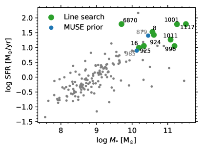
Figure 3: The stellar mass vs. SFR (from Magphys) of all galaxies with a MUSE redshift at $1.01<z<1.74$ in the ASPECS-LP footprint. Leveraging the MUSE redshift as prior, we find CO(2-1) signal in two additional galaxies (blue). The numbers indicate the MUSE IDs of the sources. The detections from the line-search (green; § 3.1) are also recovered in the prior-based search. By using the MUSE redshifts to search for CO at lower luminosities, we reveal molecular gas in most of the massive, star-forming galaxies at these redshifts.

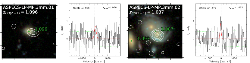
Figure 4: HST cutouts (F160W, F125W, F105W) and CO(2-1) spectra for two additional CO line candidates, found through a MUSE redshift prior. The CO contours are shown in white starting at $\pm 2\sigma$ in steps of $1\sigma$. All other labelling in the cutouts is as in Fig. 3. In the spectra the velocity is given relative to the MUSE redshift. The spectrum and best-fit Gaussian are shown in black and red, respectively. The local rms noise level is shown in green.

Table 2: ASPECS-LP CO(2-1) detected sources based on a spectroscopic redshift prior from MUSE. (1) ASPECS-LP Muse Prior (MP) ID (2)-(3) Coordinates. (4) CO line Frequency. (5) CO transition. (6) CO redshift. (7) MUSE ID. (8) MUSE redshift. (9) Velocity offset between MUSE and ALMA ($\Delta v=(z_{\rm MUSE}-z_{\rm CO})/(1+z_{\rm CO})$; after converting both to the same reference frame).

ID	R.A.	Dec.	$\nu_{\mathrm{CO}}$	CO trans.	$z_{\mathrm{CO}}$	MUSE ID	$z_{\mathrm{MUSE}}$	$\Delta v$
	(J2000)	(J2000)	(GHz)	($J_{\rm up}\rightarrow J_{\rm low}$)				km s-1
(1)	(2)	(3)	(4)	(5)	(6)	(7)	(8)	(9)
MP.3mm.01	03:32:37.30	-27:45:57.8	$109.978\pm 0.011$	$2\rightarrow 1$	1.0962	985	1.0959	$-28.2\pm 50.6$
MP.3mm.02	03:32:35.48	-27:46:26.5	$110.456\pm 0.007$	$2\rightarrow 1$	1.0872	879	1.0874	$55.8\pm 44.3$

The CO-line detections from Gonzalez-Lopez et al. (2019) are selected to have the highest fidelity and are therefore the highest S/N ($\geq 6.4$) candidates over the ASPECS-LP area. In Fig. 3, we plot the stellar mass - SFR relation for all MUSE sources at $1.01<z<1.74$, where we indicate all the galaxies that have been detected in CO(2-1) in the line search. There are several galaxies in the field with properties similar to the ASPECS-LP galaxies that are not detected in the line search. This raises the question: Why are these galaxies not detected? Given their physical properties, we may expect some of these galaxies to harbor molecular gas and therefore to have CO signal in the ASPECS-LP cube. The reason that we did not detect these sources in the line search may, therefore, simply be due to the fact that they are present at lower S/N, which puts them in the regime where the decreasing fidelity makes it challenging to identify them among the spurious sources.

However, the physical properties of the galaxies themselves provide an extra piece of information that can guide us in detecting CO for these sources. In particular, we can use the spectroscopic redshifts from MUSE to obtain a measurement of the CO flux for each source, either identifying them at lower S/N, or putting an upper limit on their molecular gas mass. We aim at the CO transitions covered at $z<2.9$, where the features in the MUSE spectrum typically provide a systemic redshift. At higher redshift the main spectral feature used to identify redshifts is often $\mathrm{Ly}\alpha$, which can be offset from the systemic redshift by a few hundred km s^-1 (e.g., Shapley et al., 2003; Rakic et al., 2011; Verhamme et al., 2018).

We extract a single-pixel spectrum from the 3″ tapered cube at the position of each MUSE source in the redshift range, after correcting for the astrometric offset (§ 2.1). We then fit the lines with a Gaussian curve, using a custom-made Bayesian Markov chain Monte Carlo routine with the following priors:

• line peak velocity: a Gaussian distribution centered at $\Delta v=0$ (based on the MUSE redshift) and $\sigma=100$ km s^-1 (the MUSE spectral resolution).

• line width: a Maxwellian distribution with a width of 100 km s^-1.

• line flux: a Gaussian distribution centered at zero, with $\sigma=0.5$ Jy km s^-1, allowing both positive and negative line fluxes to be fitted.

We choose a strong prior on the velocity difference, as we only search for lines at the exact MUSE redshift. The Gaussian prior on the line flux is important to estimate the fidelity of our measurements, allowing an unbiased comparison of positive versus negative line fluxes (see Gonzalez-Lopez et al. 2019 for details). The Maxwellian prior is chosen because it is bound to produce positive values of the line-width, depends on a single scale parameter and has a non-null tail at very large line widths. The uncertainties are computed from the 16th and 84th percentiles of the posterior distributions of each parameter.

As narrow lines are more easily caused by noise in the cube (Gonzalez-Lopez et al., 2019), we rerun the fit with a broader prior on the line width of 200 km s^-1. We also independently fit the spectrum with a uniform prior over $\pm 1$ GHz around the MUSE-redshift. We select only the sources in which the same feature was recovered with $\mathrm{S/N}>3$ in all three fits. In order to select a sample that is as pure as possible, we select only the objects that have a velocity offset of $<80$ km s^-1 from the MUSE systemic redshift ($\approx\times 2$ the typical uncertainty on the MUSE redshift). In addition, we only keep objects with a line width of $>100$ km s^-1, to avoid including spurious narrow lines. We note that, while these cuts potentially remove other sources that are detected at lower S/N, we do not attempt to be complete. Rather, we aim to have the prior-based sample as clean as possible.

The prior-based search reveals two additional sources detected in CO(2-1) with a $\mathrm{S/N}>3$. Both sources lie within the area in which the sensitivity is $>40\%$ of the primary beam peak sensitivity. We show the HST cutouts with the CO spectra of these sources in Fig. 4, ordered by S/N. ASPECS-LP-MP.3mm.02 is the foreground spiral galaxy of ASPECS-LP.3mm.08. This source was already found in the ASPECS-Pilot (Decarli et al., 2016, see Appendix A).

Because the molecular gas mass is to first order correlated with the SFR, we expect to detect CO in the galaxies with the highest SFRs at a given redshift. Sorting all the galaxies by their SFR indeed reveals a clear correlation between the SFR and the S/N in CO, suggesting there are additional sources in the ASPECS-LP datacube at lower S/N. This can also be clearly seen from Fig. 3, where our stringent sample of prior based sources all lie at log SFR[$\mathrm{M}_{\odot}$ yr^-1] $>0.5$. Qualitatively, it becomes clear that the ASPECS-LP is sensitive enough to detect molecular gas in most massive main sequence galaxies at $1.01<z<1.74$ (a quantitative discussion of the detection fraction for the full sample is provided in § 6). For many galaxies, the reason these are not unveiled in the line search may simply be because their lower CO luminosity and/or smaller line-width puts them below the conservative S/N threshold we adopt in the line search. Using the MUSE redshifts as prior information, it is possible to unveil their molecular gas reservoirs at lower S/N.

3.3 Full sample redshift distribution

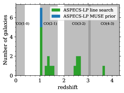
Figure 5: Redshift distribution of the ASPECS-LP CO detected sources, which all have a HST counterpart. We show both the detections from the line search (§ 3) as well as the MUSE prior based galaxies (§ 3.2). The gray shading indicates the redshift ranges over which we can detect different CO transitions.

The full ASPECS-LP CO line sample consists of 18 galaxies with a CO detection in the HUDF; 16 detections without preselection and 2 MUSE redshift prior based detections. These galaxies span a range of redshifts between $1<z<4$. The lowest redshift galaxy is detected in CO(2-1) at $z=1.04$, while the highest redshift galaxy is detected (without prior) in CO(4-3) at $z=3.60$. We show a histogram of the redshifts of the line-search and prior-based detections in Fig. 5.

Twelve sources are detected in CO(2-1) at $1.01<z<1.74$, where the combination of molecular line sensitivity and survey volume are optimal. Most prominently, we detect five galaxies at the same redshift of $z\approx 1.1$. These galaxies are all part of an overdensity of galaxies in the HUDF at $z=1.096$, visible in Fig. 1.

Five sources are detected in CO(3-2) at $2.01<z<3.11$, including the brightest CO emitter in the field at $z=2.54$ (ASPECS-LP.3mm.01; see also Decarli et al. 2016) and a pair of galaxies (ASPECS-LP.3mm.07 and #9) at $z\approx 2.697$ (see § 3.1). All five CO(3-2) sources are detected in 1 mm dust continuum (Aravena et al., 2016; Dunlop et al., 2017) with flux densities below 1 mJy. However, only one of these sources (ASPECS-LP.3mm.01) previously had a spectroscopic redshift (Walter et al., 2016; Inami et al., 2017).

4 Physical properties

4.1 Star formation rates from magphys & $\mathrm{[O\,\textsc{ii}]}$

Table 3: Physical properties of the ASPECS-LP detected sources from the line search and the MUSE prior-based search with formal uncertainties. (1) ASPECS-LP ID number. (2) Source redshift. (3) Stellar mass ($M_{*}$). (4) Star formation rate (SFR). (5) Visual attenuation ($A_{V}$). (6)–(7) X-ray classification as active galactic nucleus (AGN) or other X-ray source (X) from Luo et al. (2017) and corresponding X-ray ID (XID).

ID	$z$	$\log M_{*,\mathrm{SED}}$	SFRSED	$A_{V,\mathrm{SED}}$	X-ray	XID
		($\mathrm{M}_{\odot}$)	($\mathrm{M}_{\odot}$ yr-1)	(mag)
(1)	(2)	(3)	(4)	(5)	(6)	(7)
ASPECS-LP.3mm.01	2.5436	$10.4_{-0.0}^{+0.0}$	$233_{-0}^{+0}$	$2.7_{-0.0}^{+0.0}$	AGN	718
ASPECS-LP.3mm.02	1.3167	$11.2_{-0.0}^{+0.0}$	$11_{-0}^{+2}$	$1.7_{-0.0}^{+0.1}$
ASPECS-LP.3mm.03	2.4534	$10.7_{-0.1}^{+0.1}$	$68_{-20}^{+19}$	$3.1_{-0.3}^{+0.1}$
ASPECS-LP.3mm.04	1.4140	$11.3_{-0.0}^{+0.0}$	$61_{-12}^{+3}$	$2.9_{-0.0}^{+0.1}$
ASPECS-LP.3mm.05	1.5504	$11.5_{-0.0}^{+0.0}$	$62_{-19}^{+5}$	$2.3_{-0.3}^{+0.1}$	AGN	748
ASPECS-LP.3mm.06	1.0951	$10.6_{-0.0}^{+0.0}$	$34_{-0}^{+0}$	$0.8_{-0.0}^{+0.0}$	X	749
ASPECS-LP.3mm.07	2.6961	$11.1_{-0.1}^{+0.1}$	$187_{-16}^{+35}$	$3.2_{-0.1}^{+0.1}$
ASPECS-LP.3mm.08	1.3821	$10.7_{-0.0}^{+0.0}$	$35_{-5}^{+8}$	$0.9_{-0.1}^{+0.1}$
ASPECS-LP.3mm.09	2.6977	$11.1_{-0.0}^{+0.1}$	$318_{-35}^{+35}$	$3.6_{-0.1}^{+0.1}$	AGN	805
ASPECS-LP.3mm.10	1.0367	$11.1_{-0.1}^{+0.0}$	$18_{-1}^{+1}$	$3.0_{-0.1}^{+0.0}$
ASPECS-LP.3mm.11	1.0964	$10.2_{-0.0}^{+0.0}$	$10_{-1}^{+0}$	$0.8_{-0.1}^{+0.0}$
ASPECS-LP.3mm.12	2.5739	$10.6_{-0.1}^{+0.0}$	$31_{-3}^{+18}$	$0.8_{-0.1}^{+0.2}$	AGN	680
ASPECS-LP.3mm.13	3.6008	$9.8_{-0.1}^{+0.1}$	$41_{-9}^{+15}$	$1.4_{-0.2}^{+0.3}$
ASPECS-LP.3mm.14	1.0981	$10.6_{-0.1}^{+0.1}$	$27_{-4}^{+1}$	$1.6_{-0.2}^{+0.0}$
ASPECS-LP.3mm.15	1.0964	$9.7_{-0.0}^{+0.3}$	$62_{-4}^{+0}$	$2.9_{-0.0}^{+0.0}$	AGN	689
ASPECS-LP.3mm.16	1.2938	$10.3_{-0.0}^{+0.1}$	$11_{-3}^{+1}$	$0.5_{-0.2}^{+0.1}$
ASPECS-LP-MP.3mm.01	1.0959	$10.1_{-0.0}^{+0.1}$	$8_{-2}^{+3}$	$1.3_{-0.2}^{+0.2}$
ASPECS-LP-MP.3mm.02	1.0874	$10.4_{-0.0}^{+0.0}$	$25_{-0}^{+0}$	$1.0_{-0.0}^{+0.0}$	X	661

Table 4: Emission line flux measurements and derived unobscured SFR and metallicity for the ASPECS-LP line-search and prior-based sources at $z<1.5$ with $\mathrm{S/N}(\mathrm{[O\,\textsc{ii}]})>3$. (1) ASPECS-LP.3mm ID number. (2) MUSE ID (3) MUSE redshift. (4) $\mathrm{[O\,\textsc{ii}]}\ \lambda 3726+\lambda 3729$ flux ($\mathrm{S/N}>3$). (5) $\mathrm{[Ne\,\textsc{iii}]}\ \lambda 3869$ flux (upper limits are reported if $\mathrm{S/N}<3$). (6) SFR($\mathrm{[O\,\textsc{ii}]}\ \lambda 3726,3729$) without correction for dust attenuation. (7) Metallicity from $\mathrm{[Ne\,\textsc{iii}]}$/$\mathrm{[O\,\textsc{ii}]}$ based on Maiolino et al. (2008).

ID	MUSE ID	$z_{\mathrm{MUSE}}$	$F_{\mathrm{[O\,\textsc{ii}]}\ \lambda 3726+\lambda 3729}$	$F_{\mathrm{[Ne\,\textsc{iii}]}\ \lambda 3869}$	SFR${}_{\mathrm{[O\,\textsc{ii}]}}^{\rm no~{}dust}$	$Z_{\mathrm{[Ne\,\textsc{iii}]}/\mathrm{[O\,\textsc{ii}]},\mathrm{M08}}$
			($\times 10^{-20}\mathrm{erg\,s^{-1}\,cm^{-2}}$)	($\times 10^{-20}\mathrm{erg\,s^{-1}\,cm^{-2}}$)	($\mathrm{M}_{\odot}$ yr-1)	(12 + log(O/H))
(1)	(2)	(3)	(4)	(5)	(6)	(7)
3mm.06	8	1.0955	$111.4\pm 1.4$	$1.9\pm 0.4$	$3.59\pm 0.05$	$9.05\pm 0.08$
3mm.11	16	1.0965	$24.4\pm 0.3$	$0.9\pm 0.1$	$0.79\pm 0.01$	$8.78\pm 0.06$
3mm.14	924	1.0981	$53.6\pm 1.6$	$2.4\pm 0.4$	$1.74\pm 0.05$	$8.70\pm 0.07$
3mm.15	6870	1.0979	$13.8\pm 0.4$	$<0.2\pm 0.1$	$\cdots$	$\cdots$
3mm.16	925	1.2942	$67.0\pm 4.0$	$<1.9\pm 0.8$	$3.26\pm 0.20$	$>8.79\pm 0.17$
MP.3mm.01	985	1.0959	$17.8\pm 1.5$	$<0.6\pm 0.5$	$0.57\pm 0.05$	$>8.56\pm 0.29$
MP.3mm.02	879	1.0874	$245.9\pm 1.1$	$11.5\pm 0.6$	$7.78\pm 0.03$	$8.73\pm 0.02$
Notes. We do not compute a SFR($\mathrm{[O\,\textsc{ii}]}$) or metallicity for the X-ray detected AGN (3mm.15).

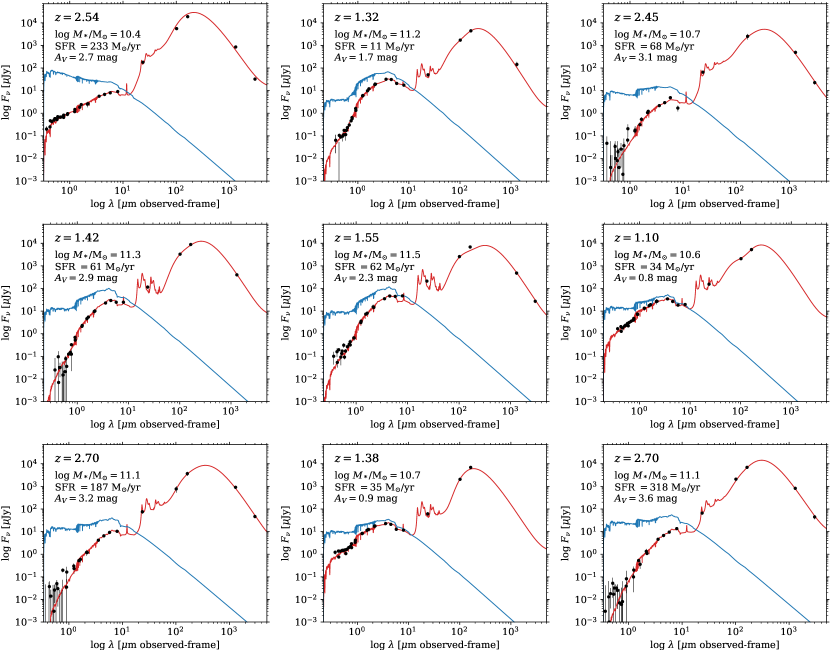
Figure 19: Spectral energy distributions (SEDs) for all the ASPECS-LP CO detected sources from the line search (first sixteen) and MUSE redshift prior based search (last two). The black points are the observed photometry. The overall best fit SED from magphys is shown by the red line, while the the model of the unattenuated stellar emission is shown in blue. The redshift and median values of the posterior likelihood distribution of the stellar mass ($M_{*}$), star formation rate (SFR) and visual attenuation ($A_{V}$) are indicated in each panel.

For all the CO detected sources, we derive the SFR (and $M_{*}$ and $A_{V}$) from the UV-FIR data (including 24µm–160µm and ASPECS-LP 1.2 mm and 3.0 mm) using Magphys (see § 2.3), which are provided in Table 3. The full SED fits are shown in Fig. 19 and 20.

For the $1<z<1.5$ subsample, we have access to the $\mathrm{[O\,\textsc{ii}]}\ \lambda 3726,3729$-doublet. We derive SFRs from $\mathrm{[O\,\textsc{ii}]}\ \lambda 3726,3729$ following Kewley et al. (2004), adopting a Chabrier (2003) IMF. The observed $\mathrm{[O\,\textsc{ii}]}$ luminosity gives a measurement of the unobscured SFR, which can be compared to the total SFR (including the FIR) to derive the fraction of obscured star formation. For that reason, we not apply a dust correction when calculating the SFR($\mathrm{[O\,\textsc{ii}]}$).

The derived SFR($\mathrm{[O\,\textsc{ii}]}\ \lambda 3726,3729$) is dependent on the oxygen abundance. We have access to the oxygen abundance directly for some of the sources and can also make an estimate through the mass-metallicity relation (e.g., Zahid et al., 2014). However, because of the additional uncertainties in the calibrations for the oxygen abundance, we instead adopt an average $\mathrm{[O\,\textsc{ii}]}\ \lambda 3726,3729$/$\mathrm{H}\alpha$ ratio of unity, given that all our sources are massive and hence expected to have high oxygen abundance $12+\log{\mathrm{O}/\mathrm{H}}$ $\sim 8.8$, where $\mathrm{[O\,\textsc{ii}]}/\mathrm{H}\alpha=1.0$ (e.g., Kewley et al., 2004). For all galaxies with S/N($\mathrm{[O\,\textsc{ii}]}\ \lambda 3726,3729$) $>3$, excluding the X-ray AGN, the $\mathrm{[O\,\textsc{ii}]}\ \lambda 3726+\lambda 3729$ line flux measurements and SFRs are presented in Table 4.

4.2 Metallicities

It is well known that the gas-phase metallicity of galaxies is correlated with their stellar mass, with more massive galaxies having higher metallicities on average (e.g., Tremonti et al., 2004; Maiolino et al., 2008; Mannucci et al., 2010; Zahid et al., 2014). For the $1.0<z<1.42$ sub-sample, we have access to $\mathrm{[Ne\,\textsc{iii}]}\ \lambda 3869$ which allows us to derive a metallicity from $\mathrm{[Ne\,\textsc{iii}]}\ \lambda 3869$/$\mathrm{[O\,\textsc{ii}]}\ \lambda 3726,3729$. We follow the relation as presented by Maiolino et al. (2008), who calibrated the $\mathrm{[Ne\,\textsc{iii}]}$/$\mathrm{[O\,\textsc{ii}]}$ line ratio against metallicities inferred from the direct $T_{e}$ method (at low metallicity; $12+\log{\mathrm{O}/\mathrm{H}}<8.35$) and theoretical models from Kewley & Dopita (2002) (at high metallicity, mainly relevant for this paper; $12+\log{\mathrm{O}/\mathrm{H}}>8.35$). Since the wavelengths of $\mathrm{[Ne\,\textsc{iii}]}\ \lambda 3869$ and $\mathrm{[O\,\textsc{ii}]}\ \lambda 3726,3729$ are close, this ratio is practically insensitive to dust attenuation. The physical underpinning lies in the fact that the ratio of the low-ionization $\mathrm{[O\,\textsc{ii}]}$ and high-ionization $\mathrm{[Ne\,\textsc{iii}]}$ lines is a solid tracer of the shape of the ionization field, given that neon closely tracks the oxygen abundance (e.g., Ali et al., 1991; Levesque & Richardson, 2014; Feltre et al., 2018). As the ionization parameter decreases with increasing stellar metallicity (Dopita et al., 2006b, a) and the metallicity of the young ionizing stars and their birth clouds is correlated, the ratio of $\mathrm{[Ne\,\textsc{iii}]}\ \lambda 3869$/$\mathrm{[O\,\textsc{ii}]}\ \lambda 3726,3729$ is a reasonable gas-phase metallicity diagnostic, albeit indirect, with significant scatter (Nagao et al., 2006; Maiolino et al., 2008) and sensitive to model assumptions (e.g., Levesque & Richardson, 2014). If an AGN contributes significantly to the ionizing spectrum, the emission lines may no longer only trace the properties associated with massive star formation. For this reason, we exclude the sources with an X-ray AGN from the analysis of the metallicity.

We report the $\mathrm{[Ne\,\textsc{iii}]}$ flux measurements and $\mathrm{[Ne\,\textsc{iii}]}$/$\mathrm{[O\,\textsc{ii}]}$ metallicities in Table 4. The solar metallicity is $12+\log{\mathrm{O}/\mathrm{H}}=8.76\pm 0.07$ (Caffau et al., 2011).

4.3 Molecular gas properties

Table 5: Molecular gas properties of the ASPECS-LP line-search and prior-based sources with formal uncertainties. The CO full-width at half maximum (FWHM) and line fluxes are taken from Gonzalez-Lopez et al. (2019). (1) ASPECS-LP ID number. (2) CO redshift. (3) Upper level of CO transition. (4) CO line FWHM. (5) Integrated line flux. (6) Line luminosity (7) CO(1-0) line luminosity assuming Daddi et al. (2015) excitation (§ 4.3). (8) Molecular gas mass assuming $\alpha_{\mathrm{CO}}=3.6$ K (km s^-1 pc²)^-1. (9) Molecular-to-stellar mass ratio, $M_{\mathrm{mol}}/M_{*}$. (10) Depletion time, $t_{\mathrm{depl}}=M_{\mathrm{mol}}/\mathrm{SFR}$.

ID	$z_{\rm CO}$	$J_{\rm up}$	FWHM	$F_{\rm line}$	$L^{\prime}_{\rm line}$	$L^{\prime}_{\rm CO(1-0)}$	$M_{\mathrm{mol}}$	$M_{\mathrm{mol}}/M_{*}$	$t_{\rm depl}$
			(km s-1)	(Jy km s-1)	($\times 10^{9}$ K km s-1 pc2)		($\times 10^{10}$ $\mathrm{M}_{\odot}$)		(Gyr)
(1)	(2)	(3)	(4)	(5)	(6)	(7)	(8)	(9)	(10)
3mm.01	2.5436	3	$517\pm 21$	$1.02\pm 0.04$	$33.9\pm 1.3$	$80.8\pm 13.8$	$29.1\pm 5.0$	$12.1\pm 2.1$	$1.2\pm 0.2$
3mm.02	1.3167	2	$277\pm 26$	$0.47\pm 0.04$	$10.7\pm 0.9$	$14.1\pm 2.1$	$5.1\pm 0.7$	$0.3\pm 0.1$	$4.5\pm 0.8$
3mm.03	2.4534	3	$368\pm 37$	$0.41\pm 0.04$	$12.8\pm 1.3$	$30.5\pm 5.9$	$11.0\pm 2.1$	$2.2\pm 0.6$	$1.6\pm 0.6$
3mm.04	1.4140	2	$498\pm 47$	$0.89\pm 0.07$	$23.2\pm 1.8$	$30.5\pm 4.3$	$11.0\pm 1.6$	$0.6\pm 0.1$	$1.8\pm 0.3$
3mm.05	1.5504	2	$617\pm 58$	$0.66\pm 0.06$	$20.4\pm 1.9$	$26.9\pm 4.0$	$9.7\pm 1.4$	$0.3\pm 0.1$	$1.6\pm 0.4$
3mm.06	1.0951	2	$307\pm 33$	$0.48\pm 0.06$	$7.7\pm 1.0$	$10.1\pm 1.7$	$3.6\pm 0.6$	$1.0\pm 0.2$	$1.1\pm 0.2$
3mm.07	2.6961	3	$609\pm 73$	$0.76\pm 0.09$	$27.9\pm 3.3$	$66.5\pm 13.6$	$23.9\pm 4.9$	$2.0\pm 0.5$	$1.3\pm 0.3$
3mm.08	1.3821	2	$50\pm 8$	$0.16\pm 0.03$	$4.0\pm 0.7$	$5.3\pm 1.2$	$1.9\pm 0.4$	$0.4\pm 0.1$	$0.5\pm 0.2$
3mm.09	2.6977	3	$174\pm 17$	$0.40\pm 0.04$	$14.7\pm 1.5$	$35.0\pm 6.8$	$12.6\pm 2.5$	$1.0\pm 0.2$	$0.4\pm 0.1$
3mm.10	1.0367	2	$460\pm 49$	$0.59\pm 0.07$	$8.5\pm 1.0$	$11.1\pm 1.9$	$4.0\pm 0.7$	$0.3\pm 0.1$	$2.2\pm 0.4$
3mm.11	1.0964	2	$40\pm 12$	$0.16\pm 0.03$	$2.6\pm 0.5$	$3.4\pm 0.7$	$1.2\pm 0.3$	$0.8\pm 0.2$	$1.2\pm 0.3$
3mm.12	2.5739	3	$251\pm 40$	$0.14\pm 0.02$	$4.8\pm 0.7$	$11.3\pm 2.5$	$4.1\pm 0.9$	$0.9\pm 0.2$	$1.3\pm 0.5$
3mm.13	3.6008	4	$360\pm 49$	$0.13\pm 0.02$	$4.3\pm 0.7$	$13.9\pm 3.4$	$5.0\pm 1.2$	$8.8\pm 2.8$	$1.2\pm 0.5$
3mm.14	1.0981	2	$355\pm 52$	$0.35\pm 0.05$	$5.6\pm 0.8$	$7.4\pm 1.4$	$2.7\pm 0.5$	$0.7\pm 0.1$	$1.0\pm 0.2$
3mm.15	1.0964	2	$260\pm 39$	$0.21\pm 0.03$	$3.4\pm 0.5$	$4.4\pm 0.8$	$1.6\pm 0.3$	$3.2\pm 1.1$	$0.3\pm 0.1$
3mm.16	1.2938	2	$125\pm 28$	$0.08\pm 0.01$	$1.8\pm 0.2$	$2.3\pm 0.4$	$0.8\pm 0.1$	$0.4\pm 0.1$	$0.7\pm 0.2$
MP.3mm.01	1.0962	2	$169\pm 21$	$0.13\pm 0.03$	$2.1\pm 0.5$	$2.8\pm 0.7$	$1.0\pm 0.2$	$0.7\pm 0.2$	$1.3\pm 0.5$
MP.3mm.02	1.0872	2	$107\pm 30$	$0.10\pm 0.03$	$1.6\pm 0.4$	$2.0\pm 0.6$	$0.7\pm 0.2$	$0.3\pm 0.1$	$0.3\pm 0.1$

The derivation of the molecular gas properties of our sources is detailed in Aravena et al. (2019). For reference, we provide a brief summary here.

We convert the observed CO($J\rightarrow J-1$) flux to a molecular gas mass ($M_{\mathrm{mol}}$) using the relations from Carilli & Walter (2013). To convert the higher order CO transitions to CO(1-0), we need to know the excitation dependent intensity ratio between the CO lines, $r_{J1}$. We use the excitation ladder as estimated by Daddi et al. (2015) for galaxies on the MS, where $r_{21}=0.76\pm 0.09$, $r_{31}=0.42\pm 0.07$ and $r_{41}=0.31\pm 0.06$ (see also Decarli et al. 2016). To subsequently convert the CO(1-0) luminosity to $M_{\mathrm{mol}}$, we use an $\alpha_{\mathrm{CO}}=3.6$ $\mathrm{M}_{\odot}$ (K km s^-1 pc²)^-1, appropriate for star-forming galaxies (Daddi et al. 2010; see Bolatto et al. 2013 for a review). This choice of $\alpha_{\mathrm{CO}}$ is supported by our finding that the ASPECS-LP sources are mostly on the MS and have (near-)solar metallicity (see § 5.4).

With these conversions in mind, the molecular gas mass and derived quantities we report here can easily be rescaled to different assumptions following: $M_{\mathrm{mol}}/\mathrm{M}_{\odot}=\left(\alpha_{\mathrm{CO}}/r_{J1}\right)L^{\prime}_{\mathrm{CO}(J\rightarrow J-1)}/$(K km s^-1 pc²).

5 Results: Global sample properties

In this section we discuss the physical properties of all the ASPECS-LP sources that were found in the line search (without preselection) and based on a MUSE redshift prior. Since the sensitivity of ASPECS-LP varies with redshift, we discuss the galaxies detected in different CO transitions separately. In terms of the demographics of the ASPECS-LP detections, we focus on CO(2-1) and CO(3-2), where we have the most detections.

5.1 Stellar mass and SFR distributions

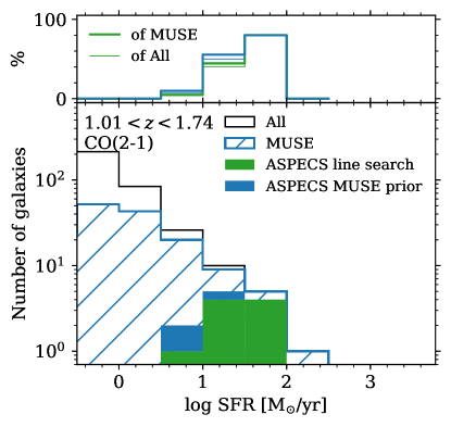
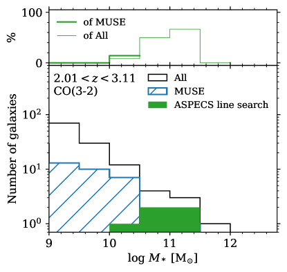
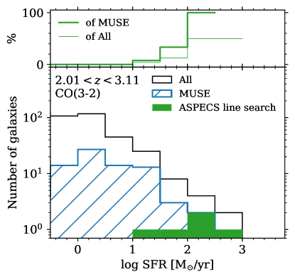
Figure 6: Histograms of the stellar mass ($M_{*}$, left) and star formation rate (SFR, right) of the ASPECS-LP detected galaxies, in comparison to all galaxies with MUSE redshifts and our extended photometric redshift catalog, in the indicated redshift range. We only show the range relevant to the ASPECS-LP detections: $M_{*}>10^{9}$ $\mathrm{M}_{\odot}$ and SFR $>0.3$ $\mathrm{M}_{\odot}$/yr. Top: CO(2-1) detected sources at $1.01<z<1.74$. Bottom: CO(3-2) detected sources at $2.01<z<3.11$. In each of the four panels, the detected fraction in both reference catalogs is shown on top (no line is drawn if the catalog does not contain any objects in that bin). With the ASPECS-LP, we detect approximately 40% of (50%) of all galaxies at $M_{*}>10^{10}$ $\mathrm{M}_{\odot}$($>10^{10.5}$ $\mathrm{M}_{\odot}$) at $1.0<z<1.7$ ($2.0<z<3.1$), respectively. In the same redshift bins, we detect approximately 60% (30%) of all galaxies with SFR $>10$ $\mathrm{M}_{\odot}$/yr ($>30$ $\mathrm{M}_{\odot}$/yr).

The majority of the detections consist of CO(2-1) and CO(3-2), at $1<z<2$ and $2<z<3$, respectively. A key question is in what part of the galaxy population we detect the largest gas-reservoirs at these redshifts.

We show histograms of the stellar masses and SFRs for the sources detected in CO(2-1) and CO(3-2) in Fig. 6. We compare these to the distribution of all galaxies in the field that have a spectroscopic redshift from MUSE and our extended (photometric) catalog of all other galaxies. In the top part of each panel we show the percentage of galaxies we detect in ASPECS, compared to the number of galaxies in reference catalogs.

We focus first on the SFRs, shown in the right panels of Fig. 6. The galaxies in which we detect molecular gas are the galaxies with the highest SFRs and the detection fraction increases with SFR. This is expected as molecular gas is a prerequisite for star formation and the most highly star-forming galaxies are thought to host the most massive gas reservoirs. The detections from the line search at $1.0<z<1.7$ alone account for $\approx 40\%$ of the galaxy population at $10<\mathrm{SFR}[\mathrm{M}_{\odot}/\mathrm{yr}]<30$, increasing to $>75\%$ at $\mathrm{SFR}>30\mathrm{M}_{\odot}/\mathrm{yr}$. Including the prior-based detections, we find 60% of the population at $\mathrm{SFR}\approx 20$ $\mathrm{M}_{\odot}$ yr^-1. Similarly, at $2.0<z<3.1$, the detection fraction is highest in the most highly star-forming bin. Notably, however, with ASPECS-LP we probe molecular gas in galaxies down to much lower SFRs as well. The sources span over two orders of magnitude in SFR, from $\approx 5$ to $>500$ $\mathrm{M}_{\odot}$ yr^-1.

The stellar masses of the ASPECS-LP detections in CO(2-1) and CO(3-2) are shown in the left panels of Fig. 6. We detect molecular gas in galaxies spanning over two orders of magnitude in stellar mass, down to $\log M_{*}[\mathrm{M}_{\odot}]\sim 9.5$. The completeness increases with stellar mass, which is presumably a consequence of the fact that more massive galaxies star-forming galaxies also have a larger gas fraction and higher SFR. At $M_{*}>10^{10}$ $\mathrm{M}_{\odot}$, we are $\approx 40\%$ complete at $1.0<z<1.7$, while we are $\approx 50\%$ complete at $M_{*}>10^{10.5}$ $\mathrm{M}_{\odot}$ at $2<z<3.1$. The full distribution includes both star-forming and passive galaxies, which would explain why we do not pick-up all galaxies at the highest stellar masses.

5.2 AGN fraction

From the deepest X-ray data over the field we identify five AGN in the ASPECS-LP line search sample (see Table 3). Two of these are detected in CO(2-1); namely, ASPECS-LP.3mm.05 and ASPECS-LP.3mm.15. The remaining three X-ray AGN are ASPECS-LP.3mm.01, 3mm.09 and 3mm.12, detected in CO(3-2). The AGN fraction among the ASPECS-LP sources is thus $2/10=20\%$ at $1.0<z<1.7$ and $3/5=60\%$ at $2.0<z<3.1$ (note that including the MUSE-prior sources decreases the AGN fraction). If we consider the total number of X-ray AGN over the field, we detect $2/6=30\%$ of the X-ray AGN at $1.0<z<1.7$ and $3/6=50\%$ at $2.0<z<3.1$, without preselection.

The comoving number density of AGN increases out to $z\approx 2-3$ (Hopkins et al., 2007). Using a volume limited sample out to $z\sim 0.7$ based on the Sloan Digital Sky Survey and Chandra, Haggard et al. (2010) showed that the AGN fraction increases with both stellar mass and redshift, from a few percent at $M_{*}\sim 10^{10.7}$ $\mathrm{M}_{\odot}$, up to $20\%$ in their most massive bin ($M_{*}\sim 10^{11.8}$ $\mathrm{M}_{\odot}$). Closer in redshift to the ASPECS-LP sample, Wang et al. (2017) investigated the fraction of X-ray AGN in the GOODS fields and found that among massive galaxies, $M_{*}>10^{10.6}\mathrm{M}_{\odot}$, $5-15\%$ and $15-50\%$ host an X-ray AGN at $0.5<z<1.5$ and $1.5<z<2.5$, respectively. The AGN fractions found in ASPECS-LP are broadly consistent with these ranges given the limited numbers and considerable Poisson error.

Given the AGN fraction among the ASPECS-LP sources (20% at $z\sim 1.4$ and 60% at $z\sim 2.6$), the question arises whether we detect the galaxies in CO because they are AGN (i.e., AGN-powered), or, whether we detect a population of galaxies that hosts a larger fraction of AGN (e.g., because the higher gas content fuels both the AGN and star-formation)? The CO ladders in, e.g., quasar host galaxies can be significantly excited, leading to an increased luminosity in the high-$J$ CO transitions compared to star-forming galaxies at lower excitation (see, e.g., Carilli & Walter, 2013; Rosenberg et al., 2015). With the band 3 data we are sensitive to the lower-$J$ transitions, decreasing the magnitude of such a bias towards AGN. At the same time, the ASPECS-LP is sensitive to the galaxies with the largest molecular gas reservoirs, which are typically the galaxies with the highest stellar masses and/or SFRs. As AGN are more common in massive galaxies, it is natural to find a moderate fraction of AGN in the sample, increasing with redshift. Once the ASPECS-LP is complete with the observations of the band 6 (1 mm) data, we can investigate the higher $J$ CO transitions for these sources and possibly test whether the CO is powered by AGN activity.

5.3 Obscured and unobscured star formation rates

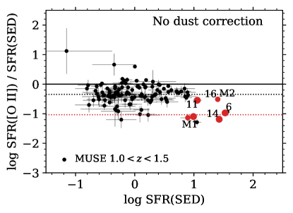
Figure 7: Total SFR from the SED fitting versus the ratio between SFR($\mathrm{[O\,\textsc{ii}]}\ \lambda 3726,3729$) and SFR(SED) for the ASPECS-LP detected sources (red) and the MUSE $1.0<z<1.5$ reference sample (black). This shows the ratio between the unobscured SFR($\mathrm{[O\,\textsc{ii}]}$) and total SFR. The black and red dotted lines show the median ratio between SFR($\mathrm{[O\,\textsc{ii}]}$) and SFR(SED) for all galaxies and the ASPECS-LP sources only. The median fraction of obscured/unobscured SFR is $10.8^{+2.3}_{-5.1}$ for all the ASPECS-LP sources.

We investigate the fraction of dust-obscured star formation by comparing the SFR derived from the $\mathrm{[O\,\textsc{ii}]}\ \lambda 3726,3729$ emission line, without dust correction, with the (independent) total SFR from modeling the UV-FIR SED with magphys. We show the ratio between the SFR($\mathrm{[O\,\textsc{ii}]}$) and the total SFR(SED) as a function of the total SFR in Fig. 7. We use the observed (unobscured) $\mathrm{[O\,\textsc{ii}]}$ luminosity, yielding a measurement of the fraction of unobscured SFR. Immediately evident is the fact that more highly star-forming galaxies (which are on average more massive) are more strongly obscured. The median ratio (bootstrapped errors) of obscured/unobscured SFR is $10.8^{+3.0}_{-5.1}$ for the ASPECS-LP sources from the line search, which have a median mass of $10^{10.6}$ $\mathrm{M}_{\odot}$ (cf. $2.2^{+0.2}_{-0.1}$ for the complete sample of MUSE galaxies, with a median mass of $10^{9}$ $\mathrm{M}_{\odot}$). Including the objects from the prior-based search does not significantly affect this fraction ($10.8^{+2.3}_{-5.1}$, at a median mass of $M_{*}\sim 10^{10.6}~{}\mathrm{M}_{\odot}$).

5.4 Metallicities at $1.0<z<1.42$

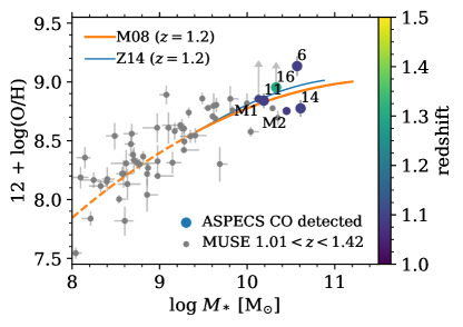
Figure 8: Stellar mass ($M_{*}$) - metallicity ($12+\log{\mathrm{O}/\mathrm{H}}$) relation for the $1<z<1.5$ sub-sample. We use the ratio of $\mathrm{[Ne\,\textsc{iii}]}\ \lambda 3869$ and the $\mathrm{[O\,\textsc{ii}]}\ \lambda 3726,3729$-doublet, available at $z<1.42$, to derive the metallicity (Maiolino et al. 2008). The solid lines show the mass-metallicity relations from Zahid et al. (2014) and Maiolino et al. (2008), (converted to the same IMF and metallicity scale, Kewley & Ellison 2008), where the latter was interpolated to the average redshift of the sample (and extrapolated to lower masses, dashed line, for reference). Overall, the ASPECS-LP galaxies are consistent with a (super-)solar metallicity.

The molecular gas conversion factor is dependent on the metallicity, which is therefore an important quantity to constrain. Specifically, $\alpha_{\mathrm{CO}}$ can be higher in galaxies with significantly sub-solar metallicities, where a large fraction of the molecular gas may be CO faint, or lower in (luminous) starburst galaxies, where CO emission originates in a more highly excited molecular medium (e.g., Bolatto et al., 2013).

Given that the majority of the ASPECS-LP sources are reasonably massive, $M_{*}\geq 10^{10}$ $\mathrm{M}_{\odot}$, their metallicities are likely to be (super-)solar, based on the mass-metallicity relation (e.g., Zahid et al., 2014).

For the ASPECS-LP sources at $1.0<z<1.42$, the MUSE coverage includes $\mathrm{[Ne\,\textsc{iii}]}\ \lambda 3869$, which can be used as a metallicity indicator (§ 4.2). We infer a metallicity for ASPECS-LP.3mm.06, 3mm.11, 3mm.14 and ASPECS-LP-MP.3mm.02. In addition, we can provide a lower limit on the metallicity for ASPECS-LP.3mm.16 and ASPECS-LP-MP.3mm.01, based on the upper limit on the flux of $\mathrm{[Ne\,\textsc{iii}]}$.

In Fig. 8, we show the ASPECS-LP sources on the stellar mass - gas-phase metallicity plane. For reference, we show the mass-metallicity relation from Maiolino et al. (2008) (that matches the $\mathrm{[Ne\,\textsc{iii}]}$/$\mathrm{[O\,\textsc{ii}]}$ calibration) and Zahid et al. (2014), both converted to the same IMF and metallicity scale (Kewley & Ellison, 2008). The AGN-free ASPECS-LP sources span about half a dex in metallicity. They are all metal-rich and consistent with a solar or super-solar metallicity, in line with the expectations from the mass-metallicity relation.

The (near-)solar metallicity of our targets supports our choice of $\alpha_{\mathrm{CO}}=3.6$ $\mathrm{M}_{\odot}$ (K km s^-1 pc²)^-1, which was derived for $z\approx 1.5$ star-forming galaxies (Daddi et al., 2010) and is similar to the Galactic $\alpha_{\mathrm{CO}}$ (cf. Bolatto et al., 2013).

6 Discussion

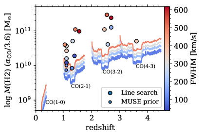
Figure 9: The $5\sigma$ molecular gas mass detection limit of ASPECS-LP as a function of redshift and CO line full-width at half-maximum (FWHM), assuming $\alpha_{\mathrm{CO}}=3.6$ and Daddi et al. (2015) excitation (see § 4.3). The sensitivity varies with redshift and increases with the square root of the decreasing line width at fixed luminosity, indicated by the color. The points indicate the ASPECS-LP blind and prior-based sources, which are detected both in the deeper and shallower parts of the sensitivity curve.

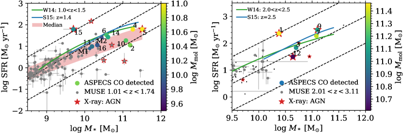
Figure 10: Stellar mass ($M_{*}$) versus SFR (from Magphys) for the CO(2-1) and CO(3-2) detected galaxies at $1.0<z<1.7$ (left) and $2.0<z<3.1$ (right), respectively. The ASPECS-LP line-search and MUSE prior-based CO detections are represented by the larger and smaller circles respectively, colored by their molecular gas mass ($M_{\mathrm{mol}}$). The gray and black points show the MUSE and photometric reference sample of galaxies, respectively. Red stars indicate X-ray sources identified as AGN from Luo et al. (2017). The green and blue solid curves denote the galaxy main sequence relationships from, respectively, Whitaker et al. (2014) and Schreiber et al. (2015). The red band shows $\pm 0.3$ dex around a polynomial fit to the running median of all galaxies in the panel. Lines of constant sSFR (0.1, 1 and 10 Gyr^-1) are shown black and dashed. At $z\sim 1.4$ ASPECS-LP detects molecular gas in galaxies that span a range of SFRs above, on and below the galaxy MS.

Figure 11: Fraction of sources detected by ASPECS-LP in $M_{*}$-SFR space at $1.01<z<1.74$ (left) and $2.01<z<3.11$ (right). This includes the detections from both the line search and the MUSE prior-based search. We are most complete at the highest SFRs and stellar masses. At a fixed stellar mass (SFR), the completeness fraction increases with SFR (stellar mass).

Figure 12: Stellar mass ($M_{*}$) versus SFR for the galaxies at $1<z<1.7$ (left) and $2<z<3.1$ (right). The ASPECS-LP detections from the full and prior-based search are represented by the larger and smaller circles respectively. The gray and black points show the MUSE and photometric reference samples of galaxies, respectively. Red stars indicate X-ray sources identified as AGN from (Luo et al., 2017). The color in the different panels denotes the change in depletion time ($t_{\mathrm{depl}}=M_{\mathrm{mol}}/\mathrm{SFR}$; top) and molecular-to-stellar mass ratio ($M_{\mathrm{mol}}/M_{*}$; bottom). The green and blue solid curves denote the MS relationships from, respectively, Whitaker et al. (2014) and Schreiber et al. (2015). The red band shows $\pm 0.3$ dex around a polynomial fit to the running median of all galaxies in the panel. Lines of constant sSFR (0.1, 1 and 10 Gyr^-1) are shown black and dashed. The gas fraction and depletion time vary systematically in galaxies across the main sequence.

6.1 Sensitivity limit to molecular gas reservoirs

Being a flux limited survey, the limiting molecular gas mass of the ASPECS-LP, $M_{\mathrm{mol}}(z)$, increases with redshift. Based on the measured flux limit of the survey, we can gain insight into what masses of gas we are sensitive to at different redshifts. The sensitivity of the ASPECS-LP Band 3 data itself is presented and discussed in Gonzalez-Lopez et al. (2019) (their Fig. 3): it is relatively constant across the frequency range, being deepest in the center where the different spectral tunings overlap.

Assuming a CO line full-width at half-maximum (FWHM) and an $\alpha_{\mathrm{CO}}$ and excitation ladder as in § 4.3, we can convert the root-mean-square noise level of ASPECS-LP in each channel to a sensitivity limit on $M_{\mathrm{mol}}(z)$. The result of this is shown in Fig. 9. With increasing luminosity distance, ASPECS-LP is sensitive to more massive reservoirs. This is partially compensated by the fact that the first few higher order transitions are generally more luminous at the typical excitation conditions in star-forming galaxies. The $M_{\mathrm{mol}}(z)$ function has a strong dependence on the FWHM, as broader lines at the same total flux are harder to detect (see also Gonzalez-Lopez et al. 2019). As the FWHM is related to the dynamical mass of the system, and we are sensitive to more massive systems at higher redshifts, these effects will conspire in further pushing up the gas-mass limit to more massive reservoirs.

At $1.0<z<1.7$, the lowest gas mass we can detect at $5\sigma$ (using the above assumptions and a FWHM for CO(2-1) of 100 km s^-1) is $M_{\mathrm{mol}}\sim 10^{9.5}$ $\mathrm{M}_{\odot}$, with a median limiting gas mass over the entire redshift range of $M_{\mathrm{mol}}\geq 10^{9.7}$ $\mathrm{M}_{\odot}$ ($M_{\mathrm{mol}}\geq 10^{9.9}$ $\mathrm{M}_{\odot}$ at FWHM = 300 km s^-1). At $2.0<z<3.1$ the median sensitivity increases to $M_{\mathrm{mol}}\gtrsim 10^{10.3}$ $\mathrm{M}_{\odot}$, assuming a FWHM of 300 km s^-1 for CO(3-2). In reality the assumptions made above can vary significantly for individual galaxies, depending on the physical conditions of their ISM.

As cold molecular gas precedes star formation, the $M_{\mathrm{mol}}(z)$ selection function of ASPECS-LP can, to first order, be viewed as a SFR$(z)$ selection function. Since more massive star-forming galaxies have higher SFRs (albeit with significant scatter), a weaker correlation with stellar mass may also be expected. These rough, limiting relations will provide useful context to understand what galaxies we detect with ASPECS.

6.2 Molecular gas across the galaxy main sequence

We show the ASPECS-LP sources in the stellar mass - SFR plane at $1.01<z<1.74$ and $2.01<z<3.11$ in Fig. 10. On average, star-forming galaxies with a higher stellar mass have a higher star formation rate, with the overall star formation rate increasing with redshift for a given mass, a relation usually denoted as the galaxy main sequence (MS). We show the MS relations from Whitaker et al. (2014, W14) and Schreiber et al. (2015, S15) at the average redshift of the sample. The typical intrinsic scatter in the MS at the more massive end is around 0.3 dex or a factor 2 (Speagle et al., 2014), which we can use to discern whether galaxies are on, above or below the MS at a given mass.

6.2.1 Systematic offsets in the MS

It is interesting to note that the average SFRs we derive with Magphys are lower than what is predicted by the MS relationships from W14 and S15 (Fig. 10). This offset is seen irrespective of including the FIR photometry to the SED fitting of the ASPECS-LP sources. This illustrates the fact that different methods of deriving SFRs from (almost) the same data can lead to somewhat different results (see, e.g., Davies et al. 2016 for a recent comparison). Both W14 and S15 derive their SFRs by summing the estimated UV and IR flux (UV+IR): W14 obtains the UV flux from integrating the UV part of their best-fit FAST SED (Kriek et al., 2009) and scales the Spitzer/MIPS 24 µm flux tot a total IR luminosity using a single template based on the Dale & Helou (2002) models. S15 instead uses (stacked) Herschel/PACS and SPIRE data for the IR luminosity, modeling these with Chary & Elbaz (2001) templates.

Recently, Leja et al. (2018) remodeled the UV–24µm photometry for all galaxies from 3D-HST survey (which were used in deriving the W14 result) using the Bayesian SED fitting code Prospector-$\alpha$ (Leja et al., 2017). While Prospector-$\alpha$ also models the broadband SED in a Bayesian framework and shares several similarities with Magphys, such as the energy-balance assumption, it is a completely independent code with its own unique features (e.g., the inclusion of emission lines, different stellar models and non-parametric star formation histories). Interestingly, the SFRs derived by Leja et al. (2018) are $\sim 0.1-1$ dex lower than those derived from UV+IR, because of the contribution of old stars to the overall energy output that is neglected in SFR(UV+IR).

While the exact nature of this offset remains to be determined, solving the systematic calibrations between different SFR indicators (or a rederivation of the MS relationship) is beyond the scope of this paper. In the following we show $\pm 0.3$ dex scatter around a second order polynomial fit to the rolling median of the SFRs all the galaxies (without any color selection) as a reference in the lower redshift bin. At the massive end where our ASPECS-LP sources lie, we indeed find that this curve lies somewhat below the W14 and S15 relationships. In the higher redshift bin the situation is less clear (given the limited number of sources) and we keep the literature references. With this description of the median SFR at a given stellar mass in hand, we are in the position to compare the SFRs of the individual ASPECS-LP sources to the population average SFR.

6.2.2 Normal galaxies at $1.01<z<1.74$

The ASPECS-LP sources at $1.01<z<1.74$ are shown in the ($M_{*}$, SFR)-plane in left panel of Fig. 10. For comparison we show all sources in this redshift range with a secure spectroscopic redshift, as MUSE is mostly complete for massive, star-forming galaxies in the regime of the ASPECS-LP detections at these redshifts (see Fig. 6).

At the depth of the ASPECS-LP, we are sensitive enough to probe molecular gas reservoirs in a variety of galaxies that lie on and even below the MS at $z\sim 1.4$. Most of the ASPECS-LP galaxies detected in this redshift range lie on the main sequence, spanning a mass range of $\sim 2$ decades at the massive end. These galaxies belong to the population of normal star-forming galaxies at these redshifts.

As expected, with the primary sample alone we detect essentially all massive galaxies that lie above the main sequence, for $M_{*}>10^{9.5}$ $\mathrm{M}_{\odot}$. The lowest mass galaxy we detect is ASPECS-LP.3mm.15, which is elevated significantly above the MS and is also an X-ray classified AGN. One galaxy, with the highest SFR of all, is a notable outlier for not being detected: MUSE#872 ($M_{*}=10^{10.2}$ $\mathrm{M}_{\odot}$, SFR $\sim 150$ $\mathrm{M}_{\odot}$ yr^-1). From the prior-based search we find that no molecular gas emission is seen in this source at lower levels either. While the non-detection of this object is very interesting, we caution that this source is also a broad-line AGN in MUSE and it is possible that its SFR is overestimated.

Notably, we also detect a number of galaxies that lie significantly below the main sequence (e.g., ASPECS-LP.3mm.02), meaning they have SFRs well below the population average. Despite their low SFR, these sources host a significant gas reservoir and have a gas fraction that is in some cases similar to MS galaxies at their stellar mass. The detection of a significant molecular gas reservoir in these sources is interesting, as these sources would typically not be selected in targeted observations for molecular gas.

Overall, we detect the majority of the galaxies on the massive end of the MS at $1.0<z<1.7$ in CO. We show the detection rate in bins of stellar mass and SFR in the left panel of Fig. 11. At a SFR $>10$ $\mathrm{M}_{\odot}$ yr^-1, we detect $>60\%$ of galaxies at all masses at these redshifts. If we focus on galaxies with $M_{*}>10^{10}\mathrm{M}_{\odot}$, we are $>60\%$ complete down to log SFR[$\mathrm{M}_{\odot}$ yr^-1] $>0.5$, where we encompass all MS galaxies.

6.2.3 Massive galaxies at $2.01<z<3.11$

At $2.01<z<3.11$, we are sensitive to CO(3-2) emission from massive gas reservoirs. We plot the galaxies detected in CO(3-2) on the main sequence in the right panel of Fig. 10. For completeness, we have added ASPECS-LP.3mm.12 to the figure as well, but caution that the photometry is blended with a lower redshift foreground source. As the number of spectroscopic redshifts from MUSE is more limited in this regime, we also include galaxies from our extended photometric redshift catalog as small black dots (indicating AGN with red stars).

The detections from ASPECS-LP make up most of the massive and highly star-forming galaxies at these redshifts. Based on their CO flux, the sources all have a molecular gas mass of $\geq 10^{10.5}$ $\mathrm{M}_{\odot}$ and correspondingly high molecular gas fractions $M_{\mathrm{mol}}/M_{*}\geq 1.0$. Their SFRs differ by over an order of magnitude. ASPECS-LP.3mm.07 and 09 are both at $z\approx 2.697$ and lie on the MS with SFRs between $150-350$ $\mathrm{M}_{\odot}$ yr^-1. In contrast, ASPECS-LP.3mm.03 has a lower SFR of $<100$$\mathrm{M}_{\odot}$ yr^-1. ASPECS-LP.3mm.01 has a very high gas fraction and SFR for its stellar mass and is also detected as an X-ray AGN.

We show the quantitative detection fraction for CO(3-2) at these redshifts in the right panel of Fig. 11. Note that, as the area of the HUDF and the ASPECS-LP is small, there are relatively few massive galaxies in the field at these redshifts.

6.3 Evolution of molecular gas content in galaxies

We now provide a brief discussion of the evolution of the molecular gas properties (and the individual outliers) in the full ASPECS-LP sample of 18 sources, including the muse prior based sources, in the context of the MUSE derived properties. A more detailed discussion of these results will be provided in Aravena et al. (2019).

From systematic surveys of the galaxy population at $z\approx 0$, we know that the molecular gas properties of galaxies vary across the main sequence (e.g., Saintonge et al., 2016, 2017). The same trends are unveiled in the ASPECS-LP sample out to $z\approx 3$. To reveal these trends more clearly, we show the main sequence plot colored by the depletion time ($t_{\rm depl}=M_{\mathrm{mol}}/\mathrm{SFR}$) and gas fraction (indicated by $M_{\mathrm{mol}}/M_{*}$) in Fig. 12. The molecular gas mass and depletion time of the ASPECS-LP sources vary systematically across the MS. On average, galaxies above the MS have higher gas fractions and shorter depletion times than galaxies on the MS, while the contrary is true for galaxies below the MS (longer depletion times, smaller gas fractions).

At $z\sim 1.4$, the sources span about an order of magnitude in depletion time, from $0.3-5$ Gyr, with a median depletion time of $\approx 1.2$ Gyr. This comparable to the average depletion times found in $z=1-3$ star-forming galaxies (e.g., Daddi et al., 2010; Tacconi et al., 2013). ASPECS-LP.3mm.02, which appears to harbor a substantial gas reservoir while its SFR puts it significantly below the main sequence, has a correspondingly long depletion time of several Gyr. Although the numbers are more limited at higher redshifts, we see a similar variety in depletion times at $z\sim 2.6$, with a median depletion time of $\approx 1.3$ Gyr. For galaxies of similar masses we do not find a strong evolution in the depletion time between the $z\sim 1.4$ and $z\sim 2.6$ bins.

The evolution of the gas fraction across the MS is clearly seen for the sources at $z\sim 1.4$. The lowest gas-mass fractions we find are of the order of 30%, while the galaxies with the highest gas fractions have about equal mass in stars and in molecular gas, with a median of $M_{\mathrm{mol}}/M_{*}\approx 0.6$. These are comparable to the gas fractions found at similar redshifts (Daddi et al., 2010; Tacconi et al., 2013). The gas fractions at $z\sim 2.6$ are substantially higher than they are at lower redshift. ASPECS-LP.3mm.09 and 12 have substantial gas fractions close to unity, while both ASPECS-LP.3mm.03 and 07, have a molecular gas mass about $\times 2$ their mass in stars (median $M_{\mathrm{mol}}/M_{*}\approx 2.0$). ASPECS-LP.3mm.1, 3mm.13 and 3mm.15 are outliers in this picture, with a substantially higher gas fraction than the other sources. Both 3mm.01 and 3mm.15 are also starbursts with a high inferred SFR and show an X-ray detected AGN. This high SFR is consistent with the high gas fraction and a picture in which the large gas reservoir fuels a strong starburst, while some gas powers the AGN simultaneously. As may be expected given the flux-limited nature of the observations, the highest redshift source, ASPECS-LP.3mm.13, also has a substantial gas fraction ($M_{\mathrm{mol}}/M_{*}=8.8\pm 2.8$). As a whole, Fig. 12 reveals the strength of the ASPECS-LP probing the molecular gas across cosmic time without preselection.

7 Summary

In this paper we use two spectroscopic integral-field observations of the Hubble Ultra Deep Field, ALMA in the millimeter, and MUSE in the optical regime, to further our understanding of the properties of the galaxy population at the peak of cosmic star formation ($1<z<3$). We start with the line emitters identified from the ASPECS-LP Band 3 (3 mm) data without any preselection (Gonzalez-Lopez et al., 2019). By using the MUSE data, as well as the deep multi-wavelength data that is available for the HUDF, we find that all ALMA-selected sources are associated with a counterpart in the optical/near-IR imaging. The spectroscopic information from MUSE enables us to associate all ALMA line emitters with emission coming from rotational transitions of carbon monoxide (CO) that result in unique redshift identifications: We identify 10 line emitters as CO(2-1) at $1<z<2$, five as CO(3-2) at $2<z<3$ and one as CO(4-3) at $z=3.6$. The line search done using the ALMA data is conservative, to avoid contamination by spurious sources in the very large 3 mm data cube (Gonzalez-Lopez et al., 2019). We therefore also use the MUSE data as a positional and redshift prior to push the detection limit of the ALMA data to greater depth and identify additional CO emitters at $z<2.9$, increasing the total number of ALMA line detections in the field to 18.

We present MUSE spectra of all CO-selected galaxies, and use the diagnostic emission lines covered by MUSE to constrain the physical properties of the ALMA line emitters. In particular, for galaxies with coverage of $\mathrm{[O\,\textsc{ii}]}\ \lambda 3727$/$\mathrm{[Ne\,\textsc{iii}]}\ \lambda 3869$ at $z\leq 1.5$ in the MUSE data, we infer metallicities consistent with being (super-)solar, which motivates our choice of a Galactic conversion factor to transform CO luminosities to molecular (H₂) gas masses for these galaxies in this series of ASPECS-LP papers (Decarli et al., 2019; Gonzalez-Lopez et al., 2019; Aravena et al., 2019; Popping et al., 2019). We also compare the unobscured $\mathrm{[O\,\textsc{ii}]}\ \lambda 3727$-derived star formation rates of the galaxies to the total SFR derived from their spectral energy distributions with Magphys and confirm that a number of them have high extinction in the rest-frame UV/optical regime.

Using the very deep Chandra imaging available for the HUDF, we determine an X-ray AGN fraction of 20% and 60% among the CO(2-1) and CO(3-2) emitters at $z\sim 1.4$ and $z\sim 2.6$, respectively, suggesting that we do not preferentially detect AGN at $z<2$. A future analysis of the band 6 data from the ASPECS-LP will reveal if those sources hosting an AGN show higher CO excitation compared to those that do not.

We use the exquisite multi-wavelength data available for the HUDF to derive basic physical parameters (such as stellar masses and star formation rates) for all galaxies in the HUDF. We recover the main sequence of galaxies and show that most of our CO detections are located towards higher stellar masses and star formation rates, consistent with expectations from earlier studies. However, being a CO-flux limited survey, besides galaxies on or above the main sequence our ALMA data also reveal molecular gas reservoirs in galaxies below the main sequence at $z\sim 1.4$, down to star formation rates of $\approx 5$ $\mathrm{M}_{\odot}$ yr^-1 and stellar masses of $M_{*}\approx 10^{10}$ $\mathrm{M}_{\odot}$. At higher redshift, we detect massive and highly star-forming galaxies in molecular gas emission on and above the MS. With our ALMA spectral scan, for stellar masses $M_{*}\geq 10^{10}(10^{10.5})$ $\mathrm{M}_{\odot}$, we detect about $40\%$ (50%) of all galaxies in the HUDF at $1<z<2$ ($2<z<3$). The ASPECS-LP galaxies span a wide range of gas fractions and depletion times, which vary with their location above, on and below the galaxy main-sequence.

The cross-matching of the integral-field spectroscopy from ALMA and MUSE has enabled us to perform an unparalleled study of the galaxy population at the peak of galaxy formation in the HUDF. Given the large range of redshifts covered by the ALMA spectral lines, key diagnostic lines in the UV/optical are only covered by the MUSE observations in specific redshift ranges. The launch of the James Webb Space Telescope will greatly expand the coverage of spectral lines that will help to further constrain the physical properties of ALMA-detected galaxies in the HUDF.

Appendix A Source description and redshift identifications

Figure 13: MUSE spectroscopy of the ASPECS-LP sources. Left: HST/F775W cutout. The colored contour(s) mark the region of the spectral extraction(s), defined by convolving the MUSE PSF with the HST segmentation map (see Inami et al. 2017 for details), or a fixed 0.8″ aperture (in the case of a new extraction; #3, #7, #9, #13). The black contours indicate the CO emission from $\pm[3,..,11]\sigma$ in steps of $2\sigma$. Right: MUSE spectrum (1.5 Å Gaussian smoothing) extracted over the marked region. The 1$\sigma$ uncertainty on the spectrum is shown by the gray line in the direction of negative flux (for clarity), and is largest around skylines. The (expected) positions of different spectral features are annotated; this does not indicate that the feature is also detected. Spectra and lines of nearby or blended sources are shown in red.

Figure 14: Continuation of Fig. 13. We show spectrum of the complete system of spiral galaxies at ASPECS-LP.3mm.08 in red (scaled down by a factor of 10), to make the faint $\mathrm{[O\,\textsc{ii}]}\ \lambda 3726,3729$ line matching the CO(2-1) redshift visible. The spectrum for ASPECS-LP.3mm.08 itself is shown in blue (extracted only over a part of the spiral arm). Note the foreground source is independently detected in CO(2-1) as ASPECS-LP-MP.3mm.02 and the fully annotated spectrum for this source is show in Fig. 15.

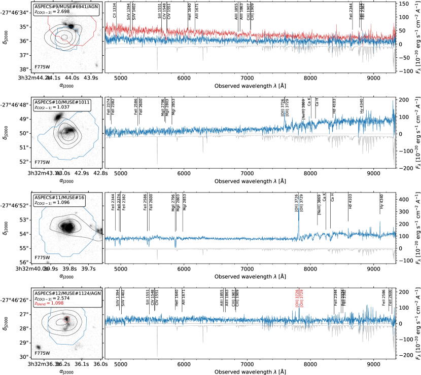
Figure 15: Continuation of Fig. 13. For ASPECS-LP.3mm.09 the UV absorption features matching the CO(3-2) redshift are seen in the source to the north (red spectrum). ASPECS-LP.3mm.12 is blended with a foreground $\mathrm{[O\,\textsc{ii}]}$-emitter (see Fig. 18).

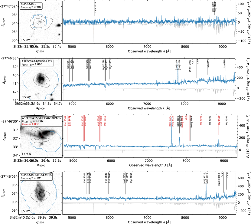
Figure 16: Continuation of Fig. 13. The spectrum of ASPECS-LP.3mm.15 is severely blended. We have highlighted the strongest blended features (from a foreground source at $z=1.038$) in red.

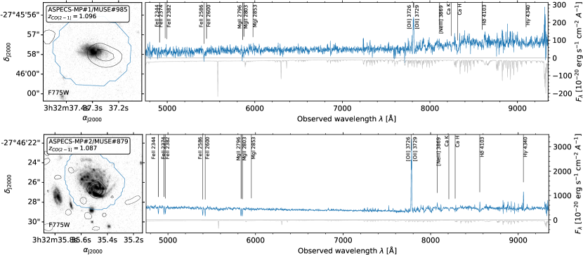
Figure 17: Continuation of Fig. 13, showing the MUSE-prior based sources.

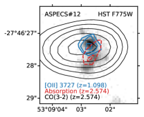
Figure 18: HST/F775W cutout of ASPECS-LP.3mm.12, with CO(3-2) emission at $z=2.5738$. The MUSE spectrum of this source reveals two redshifts. There is $\mathrm{[O\,\textsc{ii}]}$ emission at z=1.098, spatially consistent with a foreground galaxy to the north. While the continuum is faint, cross-correlating the spectrum with an absorption line template reveals a peak at $z=2.5738$ with S/N $>4$. Subsequent stacking of the UV absorption lines ($\mathrm{C\,\textsc{ii}}\ \lambda 1334$, $\mathrm{Si\,\textsc{iv}}\ \lambda 1394,1402$, $\mathrm{Si\,\textsc{ii}}\ \lambda 1551$, $\mathrm{C\,\textsc{iv}}\ \lambda 1548,1551$, $\mathrm{Al\,\textsc{ii}}\ \lambda 1671$, $\mathrm{Al\,\textsc{iii}}\ \lambda 1855,1863$) reveals that the absorption is co-spatial with the background galaxy and consistent with the redshift of CO(3-2). All contours start at $\pm 3\sigma$, increasing by $1\sigma$ (where solid and dashed indicate emission and absorption respectively).

ASPECS-LP.3mm.01: CO(3-2) at $z=2.543$. The brightest CO line emitter in the field. It is a Chandra/X-ray detected AGN (Luo et al., 2017, #718) and was already found in the line search at 3 mm and 1 mm in CO(3-2), CO(7-6) and CO(8-7) and continuum in the ASPECS-Pilot (Walter et al. 2016; Decarli et al. 2016, 3mm.1, 1mm.1, 1mm.2; Aravena et al. 2016, C1) as well as at 1 mm and 5 cm continuum (Dunlop et al., 2017; Rujopakarn et al., 2016, UDF3). The MUSE spectrum (MUSE#35) reveals a high S/N continuum with a wealth of UV absorption features and $\mathrm{C\,\textsc{iii}]}\ \lambda 1907,1909$ emission, confirming the redshift (Fig. 13). The source is a (likely interacting) pair with the source $\sim 1\farcs 5$ to the west, MUSE#24, at the same redshift ($\Delta v\approx 76$ km s^-1).

ASPECS-LP.3mm.02: CO(2-1) at $z=1.317$. Detected in both $\mathrm{[O\,\textsc{ii}]}$ and continuum in MUSE. This source is also detected in continuum at 1 mm and 5 cm (Dunlop et al., 2017; Rujopakarn et al., 2016, UDF16). $\mathrm{[O\,\textsc{ii}]}\ \lambda 3726$ is severely affected by a sky-line complicating the redshift and line-flux measurement. We remeasure the cataloged redshift for this source, which is used to compute the velocity offset with CO(2-1) (Table 1). Since we cannot confidently recover the full $\mathrm{[O\,\textsc{ii}]}$ flux, we do not include this source in the analyses of § 5.3 and § 5.4.

ASPECS-LP.3mm.03: CO(3-2) at $z=2.454$. Photometric redshift indicates $z=2-3$ (Skelton et al., 2014; Rafelski et al., 2015), perfectly in agreement with the detection of CO(3-2) at $z=2.45$. The source is faint ($m_{\mathrm{F775W}}>27$ mag) and an extraction of the MUSE spectrum yields essentially no continuum signal (see Fig. 13). This supports a redshift solution between $z=2-3$, where no bright emission lines lie in the MUSE spectral range (see § 2.2). Beside there being little continuum in the spectrum, there are no spectral features (in particular emission lines) indicative of a lower redshift ($\mathrm{[O\,\textsc{ii}]}$ at $z=1.30$) or higher redshift ($\mathrm{Ly}\alpha$ at $z=3.60$) solution. Detected in continuum at 1 mm and 5 cm (Dunlop et al., 2017; Rujopakarn et al., 2016, UDF4).

ASPECS-LP.3mm.04: CO(2-1) at $z=1.414$. MUSE spectrum shows $\mathrm{[O\,\textsc{ii}]}$ and (weak) continuum. Detected in continuum at 1 mm and 5 cm (Dunlop et al., 2017; Rujopakarn et al., 2016, UDF6).

ASPECS-LP.3mm.05: CO(2-1) at $z=1.550$. A massive ($M_{*}\approx 10^{11.5}$ $\mathrm{M}_{\odot}$) galaxy and an X-ray classified AGN (Luo et al., 2017, #748). It was also detected by the ASPECS-Pilot in 1 mm continuum (C2, Aravena et al. 2016; cf. Dunlop et al. 2017), in CO(2-1) and also CO(5-4) and CO(6-5) (ID.3, Decarli et al., 2016), and in 5 cm continuum (Rujopakarn et al., 2016, UDF8). NIR spectroscopy from the SINS survey (Förster Schreiber et al., 2009) reveals $\mathrm{H}\alpha\ \lambda 6563$, confirming the redshift we also find from MUSE, based on the $\mathrm{Fe\,\textsc{ii}}$ and $\mathrm{Mg\,\textsc{ii}}$ absorption features.

ASPECS-LP.3mm.06: CO(2-1) at $z=1.095$. Part of an overdensity in the HUDF at the same redshift. Rich star-forming spectrum in MUSE with a wealth of continuum and emission features. Detected in X-ray, but not classified as an AGN (Luo et al., 2017, #749).

ASPECS-LP.3mm.07: CO(3-2) at $z=2.696$. Photometric redshift indicates $z=2-3$ (Skelton et al., 2014; Rafelski et al., 2015), perfectly in agreement with the detection of CO(3-2) at $z=2.69$. The source is faint ($m_{\mathrm{F775W}}>27$ mag) and a reextraction of the MUSE spectrum yields essentially no continuum signal (see Fig. 14). This supports a redshift solution between $z=2-3$, where no bright emission lines lie in the MUSE spectral range (see § 2.2). Beside there being little continuum in the spectrum, there are no spectral features indicative of a lower redshift or higher redshift solution (cf. ASPECS-LP.3mm.03). There is reasonably close proximity between ASPECS-LP.3mm.07 and 09 at $z=2.69$, which are separated by only $\sim 7\farcs 5$ (60 kpc at that redshift). This object is one of the brightest sources in the HUDF at 1 mm (UDF2; Dunlop et al. 2017) and also detected at 5 cm (Rujopakarn et al., 2016).

ASPECS-LP.3mm.08: CO(2-1) at $z=1.382$. The source has a more complex morphology which was already discussed in the ASPECS-Pilot program (Decarli et al. 2016, see their Fig. 3). The CO emission is spatially consistent with a system of spiral galaxies. MUSE reveals that the south-west spiral is in the foreground at $z=1.087$. Careful examination of the MUSE cube reveals $\mathrm{[O\,\textsc{ii}]}$ emission matching the CO redshift in an arc north of the galaxies and possibly towards the south-west, which is $\sim 1.8\arcsec$ away of peak of the CO emission ($\sim 15$ kpc at the redshift of the source). A potential scenario is that the north-east spiral galaxies is the background source, in which case the ionized gas emission of the spiral is completely obscured by the disk of the (south-west) foreground spiral. This is consistent with the spatial position of the CO emission. An alternative scenario is that of a third disk galaxy harboring the CO reservoir, which is completely hidden from sight by the spiral galaxies in the foreground, except for the structures seen in the north and east. We note that resolved SED fitting of this source was recently performed by Sorba & Sawicki (2018), assuming the foreground redshift for the entire system. A clear break can be seen in the sSFR (their Figure 1.) for the northern-arm and possibly also a south-west arm; consistent with locations where $\mathrm{[O\,\textsc{ii}]}$-emission is seen. For the purpose of this paper, we associate the north-east spiral with ASPECS-LP.3mm.08 and the south-west spiral with ASPECS-LP-MP.3mm.02, but we note that this is uncertain in the case of ASPECS-LP.3mm.08. Given the limited flux we observe from the ionized gas, we do not discuss this source in that context.

ASPECS-LP.3mm.09: CO(3-2) at $z=2.698$. Photometric redshift indicates $z=2-3$ (Skelton et al., 2014; Rafelski et al., 2015), perfectly in agreement with the detection of CO(3-2) at $z=2.69$. The source is faint ($m_{\mathrm{F775W}}>27$ mag), yet, UV absorption features at $z=2.695$, matching the expected redshift of CO(3-2) at $z=2.698$, are found in the MUSE spectrum at the position of the source (see Fig. 15). The features arise in a source (MUSE#6941) $\sim 0\farcs 8$ to the north ($\sim 6.5$ kpc at $z\sim 2.7$). The spectrum of the northern source reveals a superposition of the $z=2.695$ source with a foreground galaxy at $z=1.555$. This is also suggestive from the morphology in HST, which shows a redder central clump for the northern source. Given the potential proximity of the two sources, both spatially and spectrally, ASPECS-LP.3mm.09 could be part of a pair of galaxies with the source to the north. Notably, ASPECS-LP.3mm.09 is also detected as an X-ray AGN; Luo et al. 2017, #865. Note there is also reasonably close proximity between ASPECS-LP.3mm.07 and 09 at $z=2.69$, which are separated by only $\sim 7\farcs 5$ (60 kpc at that redshift). One of the brightest sources in the HUDF at 1 mm (UDF1; Dunlop et al. 2017), also detected at 5 cm (Rujopakarn et al., 2016).

ASPECS-LP.3mm.10: CO(2-1) at $z=1.037$. The lowest redshift detection. Features a close star-forming companion at the same redshift. The MUSE spectrum shows continuum with both absorption and emission line features ($\mathrm{[O\,\textsc{ii}]}$). We reextract the spectrum with a new segmentation map to recompute the redshift and to minimize blending of the $\mathrm{[O\,\textsc{ii}]}$ flux from the close companion at slightly different redshift. The $\mathrm{[O\,\textsc{ii}]}$ line is detected in the source, but given the residual deblending uncertainties we do not take into it into account in the analyses of § 5.3 and § 5.4.

ASPECS-LP.3mm.11: CO(2-1) at $z=1.096$. Part of the overdensity in the HUDF at the same redshift. MUSE reveals a rich star-forming spectrum with stellar continuum and both absorption and emission ($\mathrm{[O\,\textsc{ii}]}$, $\mathrm{[Ne\,\textsc{iii}]}$) features.

ASPECS-LP.3mm.12: CO(3-2) at $z=2.574$. Detected in 1 mm continuum (C4; (Aravena et al., 2016)) and an X-ray AGN (Luo et al., 2017, #680). The source contains a CO line at $96.76$ GHz. The optical counterpart shows red colors in HST and features a blue component towards the north. The source is considered to be a single galaxy in most photometric catalogs (e.g., Skelton et al., 2014; Rafelski et al., 2015). However, the redshift from the MUSE catalog for this source, $z=1.098$ (based on a confident $\mathrm{[O\,\textsc{ii}]}$ detection, see Fig. 15), is incompatible with being CO(2-1), which would be at $z=1.383$. Closer inspection of the source in the MUSE IFU data reveals that the $\mathrm{[O\,\textsc{ii}]}$ emission is only originating from the blue clump to the north of the source (see Fig. 18). A reanalysis of the MUSE spectrum revealed weak absorption features that, when cross correlated with an absorption line template, correspond a redshift $z=2.5738$. Assuming that the CO line is CO(3-2) instead, this independently matches the redshift from ASPECS-LP exactly ($z=2.5738$). To further confirm that the absorption features are associated with ASPECS-LP.3mm.12, we spatially stacked narrow-bands over all strong UV absorption features (without any preselection). To construct the narrow-band, we sum the flux over each absorption feature (assuming a fixed 7Å line-width) and subtract the continuum measured in two side bands offset by $\pm 10$Å (same width in total). We then stacked the individual narrow-bands by summing the flux in each spatial pixel (note, the same result is found when taking the mean or median). The stacked absorption features have S/N $>4$ and are co-spatial with the background galaxies and the CO, confirming the detection of CO(3-2) at $z=2.5738$ (see Fig. 18).

ASPECS-LP.3mm.13: CO(4-3) at $z=3.601$. Highest redshift CO detection. It is an F435W dropout and the photometric redshifts for this source consistently suggest that it lies in the $z=3-4$ range (Skelton et al., 2014; Straatman et al., 2016), with $z_{\rm BPZ}=3.67_{-0.24}^{+0.74}$ (Rafelski et al., 2015). These all suggest a detection of CO(4-3) at $z=3.601$. In order the spectroscopically confirm this redshift, we extract a MUSE spectrum at the position of the source. The strongest UV emission line observed by MUSE at these redshifts is $\mathrm{Ly}\alpha$, while it also covers the much weaker $\mathrm{C\,\textsc{iii}]}$ line. Both are not detected in the spectrum of ASPECS-LP.3mm.13. The non-detection of $\mathrm{C\,\textsc{iii}]}$ at the 10 h depth of the mosaic is understandable, as robustly detecting $\mathrm{C\,\textsc{iii}]}$ at these redshifts is challenging (see Maseda et al. 2017 for a in-depth discussion, which finds the highest redshift detection of $\mathrm{C\,\textsc{iii}]}$ in the deep 30 h MUSE data to be at $z\sim 2.9$). Unfortunately, at $z=3.601$ the expected position of $\mathrm{Ly}\alpha$ in MUSE falls close to the $\mathrm{[O\,\textsc{i}]}\ \lambda 5577$ skyline (Fig. 16), which could explain why it is not detected. Furthermore, the source is likely to have a significant dust content in which case no $\mathrm{Ly}\alpha$ emission may be expected at all. Nevertheless, while at $m_{\mathrm{F775W}}=26.4$, the spectrum does not reveal emission or absorption lines compatible with a solution for CO(2-1) at $z=1.30$ or CO(3-2) at $z=2.45$, which suggests a higher redshift solution is appropriate for ASPECS-LP.3mm.13 (in agreement with the photo-z). In summary, the combined evidence of the photometric redshifts indicating $z\sim 3.5$ and the lack of a lower redshift solution from MUSE makes the case for the detection of CO(4-3) at $z=3.601$ in ASPECS-LP.3mm.13.

ASPECS-LP.3mm.14: CO(2-1) at $z=1.098$. Part of an overdensity in the HUDF. MUSE reveals a rich spectrum with continuum, absorption and a range of emission lines (among which $\mathrm{[O\,\textsc{ii}]}$, $\mathrm{[Ne\,\textsc{iii}]}$ and Balmer lines).

ASPECS-LP.3mm.15: CO(2-1) at $z=1.096$. Part of an overdensity in the HUDF at the same redshift. The source lies in a very crowded part of the sky with multiple galaxies at different redshifts overlapping in projection. Detected in X-rays, classified as AGN (Luo et al., 2017, #689). Source was also covered by the ASPECS-Pilot program and detected in CO(2-1) and CO(4-3) (Decarli et al., 2016, ID.5).

ASPECS-LP.3mm.16: CO(2-1) at $z=1.294$. Shows a disk-like morphology. MUSE spectrum reveals a stellar continuum with absorption, as well as emission lines ($\mathrm{[O\,\textsc{ii}]}$ and $\mathrm{[Ne\,\textsc{iii}]}$).

ASPECS-LP-MP.3mm.01: CO(2-1) at $z=1.096$. Part of an overdensity in the HUDF at the same redshift. MUSE spectrum shows stellar continuum with absorption, as well as emission lines ($\mathrm{[O\,\textsc{ii}]}$).

ASPECS-LP-MP.3mm.02: CO(2-1) at $z=1.087$. Foreground galaxy to ASPECS-LP.3mm.08, also described in Decarli et al. (2016). See ASPECS-LP.3mm.08 for a further description.

Appendix B Magphys fits for all CO detected galaxies

We performing SED fitting with magphys for all ASPECS-LP galaxies, as described in detail in § 2.3. The following bands are considered in the SED fitting of the ASPECS-LP galaxies: U₃₈ (0.37µm), IA₄₂₇ (0.43µm), F435W (0.43µm), B (0.46µm), IA₅₀₅ (0.51µm), IA₅₂₇ (0.53µm), V (0.54µm), IA₅₇₄ (0.58µm), F606W (0.60µm), IA₆₂₄ (0.62µm), IA₆₇₉ (0.68µm), IA₇₃₈ (0.74µm), IA₇₆₇ (0.77µm), F775W (0.77µm), I (0.91µm), F850LP (0.90µm), J (1.24µm), tJ (1.25µm), F160W (1.54µm), H (1.65µm), tK_s (2.15µm), K (2.21µm), IRAC (3.6µm, 4.5µm, 5.8µm, 8.0µm), MIPS (24µm), PACS (100µm and 160µm) and ALMA Band 6 (1.2 mm) and Band 3 (3.0 mm).

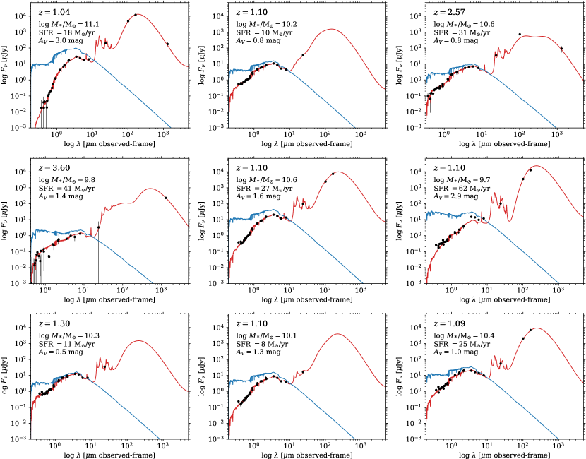
Figure 20: Continuation of Fig. 19.

References

- Akhlaghi & Ichikawa (2015) Akhlaghi, M., & Ichikawa, T. 2015, Astrophys. J. Suppl. Ser., 220, 1
- Ali et al. (1991) Ali, B., Blum, R. D., Bumgardner, T. E., et al. 1991, Publ. Astron. Soc. Pacific, 103, 1182
- Aravena et al. (2019) Aravena, M., Decarli, R., Walter, F., et al. 2019, [ASPECS LP Molecular gas paper]
- Aravena et al. (2016) Aravena, M., Spilker, J. S., Bethermin, M., et al. 2016, Mon. Not. R. Astron. Soc., 457, 4406
- Bacon et al. (2010) Bacon, R., Accardo, M., Adjali, L., et al. 2010, in Proc. SPIE, ed. I. S. McLean, S. K. Ramsay, & H. Takami, Vol. 7735, 773508
- Bacon et al. (2017) Bacon, R., Conseil, S., Mary, D., et al. 2017, Astron. Astrophys., 608, A1
- Bolatto et al. (2013) Bolatto, A. D., Wolfire, M., & Leroy, A. K. 2013, Annu. Rev. Astron. Astrophys., 51, 207
- Boogaard et al. (2018) Boogaard, L. A., Brinchmann, J., Bouché, N., et al. 2018, Astron. Astrophys., 608, A10
- Brinchmann et al. (2004) Brinchmann, J., Charlot, S., White, S. D. M., et al. 2004, Mon. Not. R. Astron. Soc., 351, 1151
- Brinchmann et al. (2008) Brinchmann, J., Kunth, D., & Durret, F. 2008, Astron. Astrophys., 485, 657
- Caffau et al. (2011) Caffau, E., Ludwig, H. G., Steffen, M., Freytag, B., & Bonifacio, P. 2011, Sol. Phys., 268, 255
- Carilli & Walter (2013) Carilli, C. L., & Walter, F. 2013, Annu. Rev. Astron. Astrophys., 51, 1
- Chabrier (2003) Chabrier, G. 2003, Publ. Astron. Soc. Pacific, 115, 763
- Chary & Elbaz (2001) Chary, R., & Elbaz, D. 2001, Astrophys. J., 556, 562
- Conroy (2013) Conroy, C. 2013, Annu. Rev. Astron. Astrophys., 51, 393
- Da Cunha et al. (2008) Da Cunha, E., Charlot, S., & Elbaz, D. 2008, Mon. Not. R. Astron. Soc., 388, 1595
- Da Cunha et al. (2015) Da Cunha, E., Walter, F., Smail, I. R., et al. 2015, Astrophys. J., 806, 110
- Daddi et al. (2010) Daddi, E., Bournaud, F., Walter, F., et al. 2010, Astrophys. J., 713, 686
- Daddi et al. (2015) Daddi, E., Dannerbauer, H., Liu, D., et al. 2015, Astron. Astrophys., 577, A46
- Dale & Helou (2002) Dale, D. A., & Helou, G. 2002, Astrophys. J., 576, 159
- Davies et al. (2016) Davies, L. J. M., Driver, S. P., Robotham, A. S. G., et al. 2016, Mon. Not. R. Astron. Soc., 485, stw1342
- Decarli et al. (2019) Decarli, R., Walter, F., Carilli, C., et al. 2019, [ASPECS LP Survey paper]
- Decarli et al. (2014) —. 2014, Astrophys. J., 782, 78
- Decarli et al. (2016) Decarli, R., Walter, F., Aravena, M., et al. 2016, Astrophys. J., 833, 70
- Dopita et al. (2006a) Dopita, M., Fischera, J., Crowley, O., et al. 2006a, Apj, 639, 788
- Dopita et al. (2006b) Dopita, M. A., Fischera, J., Sutherland, R. S., et al. 2006b, Astrophys. J. Suppl. Ser., 167, 177
- Dunlop et al. (2017) Dunlop, J. S., McLure, R. J., Biggs, A. D., et al. 2017, Mon. Not. R. Astron. Soc., 466, 861
- Eales et al. (2018) Eales, S., Smith, D., Bourne, N., et al. 2018, Mon. Not. R. Astron. Soc., 473, 3507
- Elbaz et al. (2011) Elbaz, D., Dickinson, M., Hwang, H. S., et al. 2011, Astron. Astrophys., 533, A119
- Feltre et al. (2018) Feltre, A., Bacon, R., Tresse, L., et al. 2018, Astron. Astrophys., 617, A62
- Förster Schreiber et al. (2009) Förster Schreiber, N. M., Genzel, R., Bouché, N., et al. 2009, Astrophys. J., 706, 1364
- Genzel et al. (2010) Genzel, R., Tacconi, L. J., Gracia-Carpio, J., et al. 2010, Mon. Not. R. Astron. Soc., 407, 2091
- Genzel et al. (2015) Genzel, R., Tacconi, L. J., Lutz, D., et al. 2015, Astrophys. J., 800, 20
- Gonzalez-Lopez et al. (2019) Gonzalez-Lopez, J., Decarli, R., Walter, F., et al. 2019, [ASPECS LP Line search paper]
- González-López et al. (2017) González-López, J., Bauer, F. E., Aravena, M., et al. 2017, Astron. Astrophys., 608, A138
- Haggard et al. (2010) Haggard, D., Green, P. J., Anderson, S. F., et al. 2010, Astrophys. J., 723, 1447
- Hopkins et al. (2007) Hopkins, P. F., Richards, G. T., & Hernquist, L. 2007, Astrophys. J., 654, 731
- Hunter (2007) Hunter, J. D. 2007, Comput. Sci. Eng., 9, 90
- Inami et al. (2017) Inami, H., Bacon, R., Brinchmann, J., et al. 2017, Astron. Astrophys., 608, A2
- Kewley & Dopita (2002) Kewley, L. J., & Dopita, M. A. 2002, Astrophys. J. Suppl. Ser., 142, 35
- Kewley & Ellison (2008) Kewley, L. J., & Ellison, S. L. 2008, Astrophys. J., 681, 1183
- Kewley et al. (2004) Kewley, L. J., Geller, M. J., & Jansen, R. a. 2004, Astron. J., 127, 2002
- Kriek et al. (2009) Kriek, M., van Dokkum, P. G., Labbé, I., et al. 2009, Astrophys. J., 700, 221
- Leja et al. (2018) Leja, J., Carnall, A. C., Johnson, B. D., Conroy, C., & Speagle, J. S. 2018, arXiv:1811.03637
- Leja et al. (2017) Leja, J., Johnson, B. D., Conroy, C., van Dokkum, P. G., & Byler, N. 2017, Astrophys. J., 837, 170
- Levesque & Richardson (2014) Levesque, E. M., & Richardson, M. L. A. 2014, Astrophys. J., 780, 4
- Luo et al. (2017) Luo, B., Brandt, W. N., Xue, Y. Q., et al. 2017, Astrophys. J. Suppl. Ser., 228, 2
- Maiolino et al. (2008) Maiolino, R., Nagao, T., Grazian, A., et al. 2008, Astron. Astrophys., 488, 463
- Mannucci et al. (2010) Mannucci, F., Cresci, G., Maiolino, R., Marconi, a., & Gnerucci, a. 2010, Mon. Not. R. Astron. Soc., 408, 2115
- Maseda et al. (2017) Maseda, M. V., Brinchmann, J., Franx, M., et al. 2017, Astron. Astrophys., 608, A4
- Nagao et al. (2006) Nagao, T., Maiolino, R., & Marconi, A. 2006, Astron. Astrophys., 459, 85
- Noeske et al. (2007) Noeske, K. G., Weiner, B. J., Faber, S. M., et al. 2007, Astrophys. J., 660, L43
- Oke & Gunn (1983) Oke, J. B., & Gunn, J. E. 1983, Astrophys. J., 266, 713
- Pavesi et al. (2018) Pavesi, R., Sharon, C. E., Riechers, D. A., et al. 2018, Astrophys. J., 864, 49
- Perez & Granger (2007) Perez, F., & Granger, B. E. 2007, Comput. Sci. Eng., 9, 21
- Popping et al. (2019) Popping, G., Decarli, R., Walter, F., et al. 2019, [ASPECS LP Theory paper]
- Price-Whelan et al. (2018) Price-Whelan, A. M., Sipőcz, B. M., Günther, H. M., et al. 2018, Astron. J., 156, 123
- Rafelski et al. (2015) Rafelski, M., Teplitz, H. I., Gardner, J. P., et al. 2015, Astron. J., 150, 31
- Rakic et al. (2011) Rakic, O., Schaye, J., Steidel, C. C., & Rudie, G. C. 2011, Mon. Not. R. Astron. Soc., 414, 3265
- Riechers et al. (2019) Riechers, D. A., Pavesi, R., Sharon, C. E., et al. 2019, Astrophys. J., 872, 7
- Rosenberg et al. (2015) Rosenberg, M. J., Van Der Werf, P. P., Aalto, S., et al. 2015, Astrophys. J., 801, arXiv:1501.02985
- Rujopakarn et al. (2016) Rujopakarn, W., Dunlop, J. S., Rieke, G. H., et al. 2016, Astrophys. J., 833, 12
- Saintonge et al. (2016) Saintonge, A., Catinella, B., Cortese, L., et al. 2016, Mon. Not. R. Astron. Soc., 462, 1749
- Saintonge et al. (2017) Saintonge, A., Catinella, B., Tacconi, L. J., et al. 2017, Astrophys. J. Suppl. Ser., 233, 22
- Schreiber et al. (2015) Schreiber, C., Pannella, M., Elbaz, D., et al. 2015, Astron. Astrophys., 575, A74
- Scoville et al. (2014) Scoville, N., Aussel, H., Sheth, K., et al. 2014, Astrophys. J., 783, 84
- Scoville et al. (2017) Scoville, N., Lee, N., Bout, P. V., et al. 2017, Astrophys. J., 837, 150
- Shapley et al. (2003) Shapley, a. E., Steidel, C. C., Pettini, M., & Adelberger, K. L. 2003, Astrophys. J., 588, 65
- Silverman et al. (2015) Silverman, J. D., Daddi, E., Rodighiero, G., et al. 2015, Astrophys. J. Lett., 812, L23
- Silverman et al. (2018) Silverman, J. D., Rujopakarn, W., Daddi, E., et al. 2018, Astrophys. J., 867, 92
- Skelton et al. (2014) Skelton, R. E., Whitaker, K. E., Momcheva, I. G., et al. 2014, Astrophys. J. Suppl. Ser., 214, 24
- Sorba & Sawicki (2018) Sorba, R., & Sawicki, M. 2018, Mon. Not. R. Astron. Soc., 476, 1532
- Speagle et al. (2014) Speagle, J. S., Steinhardt, C. L., Capak, P. L., & Silverman, J. D. 2014, Astrophys. J. Suppl. Ser., 214, 15
- Straatman et al. (2016) Straatman, C. M. S., Spitler, L. R., Quadri, R. F., et al. 2016, Astrophys. J., 830, 1
- Tacconi et al. (2010) Tacconi, L. J., Genzel, R., Neri, R., et al. 2010, Nature, 463, 781
- Tacconi et al. (2013) Tacconi, L. J., Neri, R., Genzel, R., et al. 2013, Astrophys. J., 768, 74
- Tacconi et al. (2018) Tacconi, L. J., Genzel, R., Saintonge, A., et al. 2018, Astrophys. J., 853, 179
- Taylor (2005) Taylor, M. B. 2005, Astron. Data Anal. Softw. Syst. XIV - ASP Conf. Ser., 347, 29
- The Astropy Collaboration et al. (2013) The Astropy Collaboration, Robitaille, T. P., Tollerud, E. J., et al. 2013, Astron. Astrophys., 558, A33
- Tremonti et al. (2004) Tremonti, C. a., Heckman, T. M., Kauffmann, G., et al. 2004, Astrophys. J., 613, 898
- Van Der Walt et al. (2011) Van Der Walt, S., Colbert, S. C., & Varoquaux, G. 2011, Comput. Sci. Eng., 13, 22
- Verhamme et al. (2018) Verhamme, A., Garel, T., Ventou, E., et al. 2018, Mon. Not. R. Astron. Soc. Lett., 478, L60
- Walter et al. (2014) Walter, F., Decarli, R., Sargent, M., et al. 2014, Astrophys. J., 782, 79
- Walter et al. (2016) Walter, F., Decarli, R., Aravena, M., et al. 2016, Astrophys. J., 833, 67
- Wang et al. (2017) Wang, T., Elbaz, D., Alexander, D. M., et al. 2017, Astron. Astrophys., 601, A63
- Whitaker et al. (2014) Whitaker, K. E., Franx, M., Leja, J., et al. 2014, Astrophys. J., 795, 104
- Xue et al. (2011) Xue, Y. Q., Luo, B., Brandt, W. N., et al. 2011, Astrophys. Journal, Suppl. Ser., 195, arXiv:1611.03501
- Zahid et al. (2014) Zahid, H. J., Dima, G. I., Kudritzki, R.-P., et al. 2014, Astrophys. J., 791, 130