The Ly$\alpha$ Luminosity Function and Cosmic Reionization at $z\sim$ 7.0:
a Tale of Two LAGER Fields

Abstract

We present the largest-ever sample of 79 Ly$\alpha$ emitters (LAEs) at $z\sim$ 7.0 selected in the COSMOS and CDFS fields of the LAGER project (the Lyman Alpha Galaxies in the Epoch of Reionization). Our newly amassed ultradeep narrowband exposure and deeper/wider broadband images have more than doubled the number of LAEs in COSMOS, and we have selected 30 LAEs in the second field CDFS. We detect two large-scale LAE-overdense regions in the COSMOS that are likely protoclusters at the highest redshift to date. We perform injection and recovery simulations to derive the sample incompleteness. We show significant incompleteness comes from blending with foreground sources, which however has not been corrected in LAE luminosity functions in the literature. The bright end bump in the Ly$\alpha$ luminosity function in COSMOS is confirmed with 6 (2 newly selected) luminous LAEs (L_Lyα $>$ 10^43.3 erg s^-1). Interestingly, the bump is absent in CDFS, in which only one luminous LAE is detected. Meanwhile, the faint end luminosity functions from the two fields well agree with each other. The 6 luminous LAEs in COSMOS coincide with 2 LAE-overdense regions, while such regions are not seen in CDFS. The bright-end luminosity function bump could be attributed to ionized bubbles in a patchy reionization. It appears associated with cosmic overdensities, thus supports an inside-out reionization topology at $z$ $\sim$ 7.0, i.e., the high density peaks were ionized earlier compared to the voids. An average neutral hydrogen fraction of $x_{HI}$ $\sim$ 0.2 – 0.4 is derived at $z\sim$ 7.0 based on the cosmic evolution of the Ly$\alpha$ luminosity function.

1. Introduction

Cosmic reionization is a critical epoch in the history of the universe, during which most of the neutral hydrogen is ionized by the hard UV photons arising from the star forming galaxies and active galactic nuclei (AGNs). Observations of the Gunn-Peterson troughs in the quasar spectra show that the epoch of reionization (EoR) ends at $z\sim 6$ (Fan et al. 2006). Meanwhile, Planck Collaboration et al. (2018) derived a mid-point reionization redshift $z\sim 7.7\pm 0.7$ through measuring the Thompson scattering of CMB photons from free electrons. High-$z$ gamma ray bursts (GRBs), quasars and galaxies are also probes to constrain the evolution of the neutral hydrogen fraction in the intergalactic medium (e.g. Greiner et al. 2009; Mortlock et al. 2011; Bañados et al. 2018; Finkelstein et al. 2015; Bouwens et al. 2015); however, the constraints are still poor up to date, especially at $z\gtrsim 7$.

Ly$\alpha$ emitters (LAEs) are powerful probes to investigate cosmic reionization, as Ly$\alpha$ photons from galaxies in the early universe are resonantly scattered by the neutral hydrogen atoms in the intergalactic medium (IGM), and thus are sensitive to the neutral hydrogen fraction $x_{\mathrm{H\,\textsc{i}}}$ (for a review see Dijkstra 2014). High redshift LAEs can be effectively selected with narrowband imaging surveys (e.g. Malhotra & Rhoads 2004; Hu et al. 2010; Ouchi et al. 2010; Tilvi et al. 2010; Hibon et al. 2010, 2011, 2012; Krug et al. 2012; Konno et al. 2014; Matthee et al. 2015; Santos et al. 2016; Konno et al. 2018). In the past two decades, more than a thousand of LAE candidates have been selected at $z\sim 5.7$, $6.5$, and $6.6$ (e.g. Konno et al. 2018; Jiang et al. 2017). However, very small number of LAEs at $z\gtrsim 7$ had beed selected. So far before this study, the largest samples of LAEs at $z\gtrsim 7$ include three ones at $z$ $\sim$ 7.0, i.e., the 23 candidates by Zheng et al. (2017), 20 candidates by Ota et al. (2017) and 34 candidates by Itoh et al. (2018).

Lyman Alpha Galaxies in the Epoch of Reionization (LAGER) is an ongoing large area narrowband imaging survey for LAEs at $z\sim 7.0$, using the Dark Energy Camera (DECam) installed on the Cerro Tololo Inter-American Observatory (CTIO) Blanco 4-m telescope. DECam, with a red-sensitive 520 Megapixel camera and pixel scale of $0.27\arcsec$ and a superb field of view (FoV) of $\sim 3$ deg², is one of the best instruments in the world to conduct such surveys. A custom-made narrowband filter NB964 (with central wavelength $\sim$ 9642Å and FWHM $\sim$ 92Å, see Fig. 1) was installed in the DECam system in December 2015 to search for LAEs at $z$ $\sim$ 7.0. The narrowband filter bandpass was optimally designed to avoid strong sky OH emission lines and atmospheric absorption (see the transmission of NB964 filter and sky OH emission in Fig. 1, for more details please see Zheng et al. 2019).

In the first LAGER field COSMOS, we selected 23 $z\sim 7.0$ LAE candidates with 34 hours NB964 exposure (in the central $2$ deg² region; Zheng et al. 2017). A bright end bump in the Ly$\alpha$ LF is revealed, suggesting the existence of ionized bubbles in a patchy reionization process. Six of the LAE candidates have been spectroscopically confirmed (Hu et al. 2017), including 3 luminous LAE with Ly$\alpha$ luminosities of $\sim 10^{43.5}$ erg s^-1.

In this paper, we present new results of $z\sim 7.0$ LAEs selected in the deeper LAGER-COSMOS field and a second LAGER-CDFS field. In §2, we describe the observations and data reduction. We present the LAE selection in §3. The sample completeness and the derived Ly$\alpha$ LF are given in §4. In section 5, we discuss the evolution of Ly$\alpha$ LF and the cosmic reionization at $z\sim 7.0$. Throughout this work, we adopt a flat $\Lambda$CDM cosmology with $\Omega_{\mathrm{m}}=0.3$, $\Omega_{\mathrm{\Lambda}}=0.7$ and H${}_{0}=70$ km s^-1 Mpc^-1.

2. Observations and Data Reduction

2.1. Observations

Table 1Summary of Imaging Observations

Filter	$\lambda_{c}$a (Å)	$\Delta\lambda$b (Å)	Exp. Time (s)	PSF Size (arcsec)	5$\sigma$ Limiting Magnitude (AB) 2″/1.35″(aperture diameter)	Observation Dates and Notes
COSMOS
NB964	9642.0	92.0	170,100	0.90	25.2/25.7	2015 Dec 8, 2016 Feb 4-9, Mar 9-12, 2017 Dec 24-27
SSC-$B$	4458.3	851.1	$*$	0.61	27.7/28.1	Public data
HSC-$g$	4816.1	1382.7	8,400	0.92	28.0/28.5	Public data (Aihara et al. 2018; Tanaka et al. 2017)
HSC-$r$	6234.1	1496.6	5,400	0.57	27.7/28.2	Public data (Aihara et al. 2018; Tanaka et al. 2017)
HSC-$r^{c}$	6234.1	1496.6	$*$	0.63	26.0/26.5	Public data (Aihara et al. 2018)
HSC-$i$	7740.6	1522.2	21,600	0.63	27.5/27.9	Public data (Aihara et al. 2018; Tanaka et al. 2017)
HSC-$z$	9125.2	770.1	12,600	0.64	26.7/27.1	Public data (Aihara et al. 2018; Tanaka et al. 2017)
HSC-$y$	9779.9	740.5	34,200	0.81	26.2/26.6	Public data (Aihara et al. 2018; Tanaka et al. 2017)
CDFS
NB964	9642.0	92.0	121,200	0.97	25.0/25.5	2015 Dec 7 & 23, 2016 Mar 9-12, 2016 Nov 19-20, 2017 Dec 24-27
DECam-$g$	4734.0	1296.3	47,000	1.33	27.5/28.0	Public data from NOAO Archive
DECam-$r$	6345.2	1483.8	161,750	1.20	27.6/28.0	Public data from NOAO Archive
DECam-$i$	7749.6	1480.6	105,450	1.10	27.3/27.8	Public data from NOAO Archive
DECam-$z$	9138.2	1478.7	274,680	1.02	27.0/27.5	Public data from NOAO Archive

• ^a Central wavelength of the filter.

• ^b Effective width (FWHM) of the filter.

• ^c From HSC SSP deep survey. Note other HSC images are from HSC SSP ultra-deep survey.

Our DECam NB964 exposures of two LAGER fields were obtained between Dec. 2015 to Dec. 2017. The total exposure time is 47.25 hrs in COSMOS and 32.9 hrs in CDFS. The NB964 data were scientifically reduced and calibrated by DECam Community Pipeline (Valdes et al. 2014), and the individual DECam frames were stacked with our customized pipeline (see §2.2).

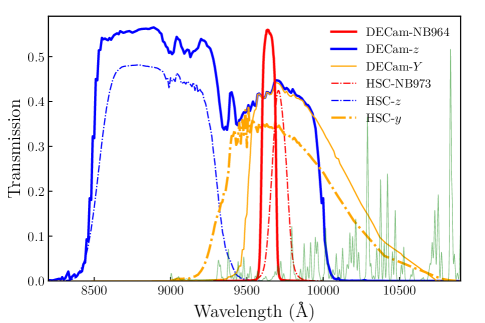
Figure 1.— Total transmission curves of DECam filters and HSC filters, including the full system response from atmosphere (at airmass of $1.2$) to detector. The underlying broad bands (DECam-$z$ for CDFS and HSC-$y$ for COSMOS) adopted in this work are shown as bolded lines. The HSC-NB973 (Itoh et al. 2018) is over-plotted for direct comparison with NB964 on DECam. The sky OH emission lines are also plotted (green line).

In COSMOS, the recently released Hyper Suprime-Cam Subaru Strategic Program (HSC-SSP) ultra deep broadband images ($grizy$, Tanaka et al. 2017) are considerably deeper than the public DECam broadband images and the Subaru Suprime-Cam (SSC) images we used in Zheng et al. (2017). In this work we use the ultradeep HSC-SSP broadband images for LAE selections, and the deep SSC-$B$ band image is kept to extend the blue wavelength coverage down to 3500Å. The merged HSC observations of COSMOS by SSP team and University of Hawaii (Aihara et al. 2018; Tanaka et al. 2017) were downloaded from HSC-SSP archive. HSC-$y$ band is selected as the underlying broadband (see Fig. 1 for the total transmission curve) for comparison with NB964 narrowband for emission line selection.

In CDFS, ultradeep DECam broadband exposures ($griz$, together with much shallower $u$ and $Y$ exposures) are available and downloaded from National Optical Astronomy Observatory (NOAO) Science Archive. DECam-$Y$ image is however too shallow. We opt to intend use DECam-$z$ as the underlying broadband. Its bandpass, unlike that of HSC-$z$, does overlap with NB964 (see Fig. 1 for the total transmission curve). The broadband DECam exposures were also stacked as described in §2.2. Note the total transmission curves of DECam filters in Fig. 1 are higher than those of HSC filters. This is mainly because the CCD detector of DECam (Diehl et al. 2008) has better quantum efficiency in the near-infrared than that of HSC.

All the broadband and narrowband images used in this paper, including the 5$\sigma$ limiting magnitudes (for 2″ and 1.35″ diameter aperture respectively), are listed in Tab. 1.

2.2. Image stacking

In this section, we describe our optimal weighted-stacking approach following Annis et al. (2014) and Jiang et al. (2014). Briefly, for each individual DECam frame, we obtain the PSF, atmospheric transmission, and exposure time to generate a weight mask using those parameters and weight map provided by DECam Community Pipeline. Below are details of the approach.

Firstly, we use PSFEx (Bertin 2011) to extract the PSF of each image and run SExtractor (Bertin & Arnouts 1996) to detect objects in the image. To perform relative photometric calibration, we take one photometric frame for each band with low PSF FWHM as a standard image, and select a set of bright, unsaturated point-like sources as standard stars. We obtain the zero-point of each frame relative to the standard image through cross-matching the standard stars in the images with a matching radius of $1\arcsec$. We use these zero-point offsets to normalize the images to the same flux level.

We utilize a 4$\sigma$-clipping method to reject artifacts in each frame (i.e., satellite trails, meteors, etc) which have not been masked out by the bad pixels masks provided by DECam Community Pipeline. Since PSF varies in different images which will affect the clipping, we allow a fraction of 30% flux variation per pixel during the clipping.

We assign each exposure a weight based on their exposure time $t_{i}$, PSF $\mathrm{FWHM}_{i}$, atmospheric transmission $T_{i}$, and background variance $\sigma_{i}^{2}$:

$$w_{i}=\frac{T^{2}_{i}t^{2}_{i}}{\mathrm{FWHM}^{2}_{i}\sigma^{2}_{i}}.$$ (1)

This is similar to inverse variance weighting to minimize the variance of stacked image. Here, the background variance $\sigma^{2}_{i}$ is given by DECam Community Pipeline, named wtmap, which is the inverse variance of the local background. The atmospheric transmission $T_{i}$ is calculated with the relative zero-point of each individual frame aforementioned.

Finally, we use SWarp (Bertin et al. 2002) to resample and stack flux-normalized images with weight masks, and we obtain a stacked science image and a composite weight map.

2.3. Photometric Calibration

We use SExtractor dual-image mode to extract sources from the images and measure photometry. The magnitude zero-points of broadband images in CDFS and COSMOS are calibrated using DES DR1 catalog (Abbott et al. 2018) and COSMOS/UltraVISTA catalog (Muzzin et al. 2013), respectively. The NB964 images are photometrically calibrated with $\sim 900$ A and B type stars in each field. More specifically, we use Python package SED Fitter (Robitaille et al. 2007) to perform spectral energy distribution fitting to the broadband photometries of stars with Castelli & Kurucz (2004) models (Castelli & Kurucz 2004), and then convolve the spectra with NB964 transmission curve to calculate the magnitudes of these stars in NB964 images.

3. LAE candidates

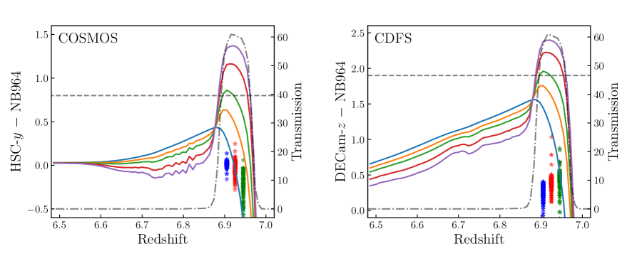
Figure 2.— Expected underlying BB $-$ NB964 color for LAEs from $z\sim 6.5$ to $7.0$. Blue, orange, green, red, and purple lines present the colors of LAEs with rest frame Ly$\alpha$ EWs of 0, 5, 10, 20, 30Å, respectively. Grey dash-dotted lines show the profile of our NB964 filter. The grey dashed lines show the color cut we used for selecting LAEs, 1.9 for CDFS field and 0.8 for COSMOS field. We also plot the expected colors of the M/L/T dwarfs (in blue, red and green stars) using the spectra from SpeX Prism Library. Note that the $x$-axis values for dwarfs are artificial.

3.1. Selection Criteria

Our selection criteria of $z$ $\sim$ 7.0 LAEs consist of three components: 1) significant detection in NB964 image; 2) color-excess of NB964 relative to the underlying broadband; and 3) non-detection in the bluer broadband (veto band) to filter out foreground galaxies.

We require our LAE candidates to be detected in NB964 image with signal-to-noise ratio (SNR) $>$ 5 in 2″ diameter aperture. In order to rule out “diffuse” artificial signals in the images, we find it is useful to further apply a cut of SNR $>$ 5 in a 1.35″ aperture. The completeness of such detection criteria is more complex than a single aperture photometry cut, but can still be estimated with injection and recovery simulations (see §4.1).

NB964 selected LAEs at $z$ $\sim$ 7.0 would exhibit flux excesses between the narrowband and the underlying broad band images (HSC-$y$ for COSMOS, and DECam-$z$ for CDFS). To estimate the color excess, we simulate the photometric properties of $z\sim 7$ LAEs from model spectrum following Itoh et al. (2018). We assume a $\delta$-function-like Ly$\alpha$ line profile and power-law UV continuum ($f_{\lambda}\propto\lambda^{\beta}$ with $\beta=-2$). The UV spectra are attenuated by the neutral IGM with the model from Madau (1995). We convolve the model spectrum with filter transmission (convolved with instrument response and atmospheric transmission, hereafter the same) to calculate the expected color excess for $z$ $\sim$ 6.5 – 7.0 LAEs with various Ly$\alpha$ line equivalent widths. As shown in Fig. 2, we adopt color cuts of BB – NB $>$ $1.9$ and $0.8$ for DECam-$z$ and HSC-$y$, respectively, corresponding to rest-frame EW₀ of Ly$\alpha$ line $\geqslant 10\mathrm{\AA}$. Following Ota et al. (2017), we also plot the expected colors of the M/L/T dwarfs using the spectra from SpeX Prism Libarary to examine whether dwarfs could be selected with our color cuts. Clearly, none of these dwarfs satisfies our criteria.

For COSMOS, we select LAEs using NB964 and Subaru HSC-$g,r,i,z,y$ Ultra-deep plus SSC-$B$ images with the following criteria:

$$\begin{split}&\mathrm{SNR_{2\arcsec}(NB964)>5\;\&\ SNR_{1.35\arcsec}(NB964)>5};\\ &\&\ \mathrm{SNR_{1.35\arcsec}(}B,g,r,i,z\mathrm{)<3};\\ &\&\ \mathrm{[(}y\mathrm{-NB964>0.8\ \&\ SNR_{1.35\arcsec}(}y\mathrm{)>3)\ or}\\ &\mathrm{SNR_{1.35\arcsec}(}y\mathrm{)<3]},\end{split}$$ (2)

Here we utilize SExtractor AUTO magnitudes (measured with dual imaging model on NB and BB) to calculate the color excess, as it is known the Ly$\alpha$ emission in LAEs is more extended than the UV continuum (e.g. Momose et al. 2016; Yang et al. 2017; Leclercq et al. 2017). In such case, the AUTO magnitudes, measured within regions defined by the narrowband image, could better recover the intrinsic color comparing with the common approach using aperture magnitudes (PSF-matched) to measure the color (see Appendix A for detailed comparison).

We note that sources with SNR${}_{1.35\arcsec}(y)$ $<$ 3 automatically satisfy the color excess criterion ($y$ - NB964 $>$ 0.8), as the the underlying broadband image is much deeper than the narrowband image (see also Fig. 3).

After masking out regions with significant CCD artifacts and bright stellar halos, we select LAEs in the central region of NB964 exposure for which the NB964 image is covered with HSC-$y$ ultradeep exposure (with a total effective sky area of 1.90 deg²). For a small region of 0.45 deg² with no coverage of HSC-$r$ Ultra-deep exposure, we employ HSC-$r$ deep data from Aihara et al. (2018). All HSC and SSC images are resampled to match DECam pixel scale.

Similarly, for CDFS, we select LAEs using NB964 and DECam-$u,g,r,i,z$ band with selection criteria:

$$\begin{split}&\mathrm{SNR_{2\arcsec}(NB964)>5\ \&\ SNR_{1.35\arcsec}(NB964)>5};\\ &\&\ \mathrm{SNR_{2\arcsec}(}u,g,r,i\mathrm{)<3};\\ &\&\ \mathrm{[(}z\mathrm{-NB964>1.9\ \&\ SNR_{2\arcsec}(}z\mathrm{)>3)\ or}\\ &\mathrm{SNR_{2\arcsec}(}z\mathrm{)<3]},\end{split}$$ (3)

Again, sources with SNR${}_{2\arcsec}(y)$ $<$ 3 automatically satisfy the color excess criterion ($y$ - NB964 $>$ 1.9, see also Fig. 3). Since DECam broadband images were obtained without significant dithering, we lost a significant portion of sky coverage due to CCD gaps. The final selection was performed in a total effective area of 2.14 deg² with both deep broad and narrowband coverage.

Note we adopt 2″ aperture for veto band photometry in CDFS, but 1.35″ aperture for COSMOS. This is because COSMOS broadband images generally have better seeing than those in CDFS. We find the 2″ aperture veto band photometry of some good candidates would be contaminated by nearby foreground sources. Measuring photometry with 1.35″ aperture avoids the loss of such candidates. We note blending with foreground galaxies in the veto bands can still yield significant incompleteness in the final selected LAE sample, which we calculate with injection and recovery simulations in §4.1 and correct in the calculation of our luminosity function.

3.2. Selected Candidates

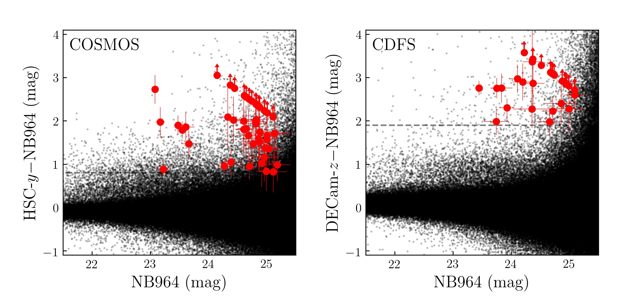
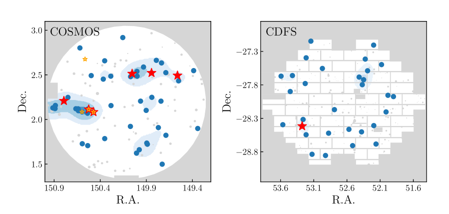
Figure 3.— Upper panel: the color-magnitude diagrams (HSC-$y-$NB964 vs. NB964 for COSMOS and DECam-$z-$NB964 vs. NB964 for CDFS) of the LAE candidates (in red) and all other objects (in black). The dashed lines are the color criteria we used to select LAEs. Bottom panel: the spatial distribution of the selected LAEs in COSMOS and CDFS (blue dots). The luminous LAEs with $\log_{10}\mathrm{L}>43.3$ are marked with red stars. The four luminous LAEs selected by Itoh et al. (2018) are over-plotted with orange stars. The blue shadow contours show the local number densities of LAEs smoothed with a Gaussian Kernel of $\sigma=0.1\deg$ to highlight the overdense regions, with the contour levels respect to [1,2,3]$\times$ average number density of LAEs in the COSMOS and CDFS field. The regions we masked out when we perform candidate selections, completeness analyses and LF calculations are marked with grey shades. Note in CDFS as the archive broadband data were obtained without dithering, we exclude regions in CCD gaps. Spectroscopic confirmations of 6 LAES in the COSMOS field have beed reported by Hu et al. (2017), including the 3 luminous ones at the left side. More spectroscopic confirmations will be presented in future works.

A sample of 75 and 50 likely candidates were selected in COSMOS and CDFS respectively after excluding tens that were identified as obviously artificial due to CCD artifacts, stellar halos, bleeding trails, and significant veto band signals in quick visual examinations. 3 transients were further excluded in COSMOS using NB964 exposures obtained at different epochs. We then perform a careful visual inspection of the candidates. Although we adopt 3$\sigma$ rejection in veto bands, 11 and 12 candidates in COSMOS and CDFS show weak counterparts in at least one of the veto broadbands and are excluded. These sources are more likely foreground transients or extreme emission line galaxies (see also §3.3). We also remove 10 and 8 candidates in COSMOS and CDFS whose NB964 signals appear more like weak CCD artifacts or noise spikes, or are too close to adjacent bright objects. Though such steps are somehow subjective, inspections from various team members often yield consistent classifications, and slight inconsistencies from various inspectors do not significantly alter the scientific results presented in this work. As foreground emission line galaxies (ELGs) may trace the overdense regions (e.g. Hayashi et al. 2018), we further reject 2 candidates in COSMOS field which are adjacent to foreground ELGs (those NB964 excess sources with veto band detections) within $3\arcsec$.

We then examine the stacked veto band images (which is deeper than a single veto band) of the remaining candidates, and none of them show signal to noise ratio $>$ 2 in the stacked veto band. Finally, we obtain a clean sample of 49 and 30 LAE candidates in COSMOS and CDFS field respectively, the thumbnail images of which are presented in Appendix B, and the catalog will be released in a future work, together with candidates to be selected in upcoming new LAGER fields. In Fig. 3 we plot the color-magnitude diagrams and the spatial distribution of our selected LAEs in COSMOS and CDFS, in which two possible elongated over dense regions are seen in COSMOS. Each has a 2 dimensional scale of $\sim$ 75 $\times$ 40 cMpc², and contains $\sim$ 12 LAEs, including 3 of which are luminous with L_Lyα $>$ 10^43.3 erg s^-1. Such large scale structures of high redshift LAEs probe the protoclusters in the early universe, and have been reported at redshift of 5.7 and 6.6 (Wang et al. 2005; Ouchi et al. 2005; Jiang et al. 2018; Harikane et al. 2019) and smaller (Shimasaku et al. 2003; Zheng et al. 2016). We note that 5 members of the large scale structures have been spectroscopically confirmed using Magellan/IMACS (Hu et al. 2017), with a remarkably high success rate of 2/3, This indicates these two structures are physically real. Spectroscopic followup of the remaining members is ongoing to further secure their identifications, and will be presented in future work.

Using 34 hr NB964 exposure, overlapping UltraVISTA Y band image, and deep Subaru SSC broadband images in the central 2 deg² region, Zheng et al. (2017) selected 23 LAEs at $z$ $\sim$ 7.0 with EW $\geqslant 10\mathrm{\AA}$. Among them, 21 were recovered in this work using 47.25 hr NB964 exposure and considerably deeper broadband images. One of the other two was detected in the 47.25 hr NB964 image with S/N $<$ 5.0. It is a transient source, as the NB964 signal disappears in the latest 13.25 hr exposure. The final one passed the selection criteria, but was also rejected as a variable source with new NB964 data.

The total LAEs selected in COSMOS in this work is 49, more than doubling the number of Zheng et al. (2017). Among the 28 new LAE candidates selected in this work but not in Zheng et al. (2017), 10 had NB964 S/N $<$ 5 in the 34hr exposure image; 7 had no SSC broadband coverage; 6 had too shallow or noisy broadband coverage; 1 was contaminated by a nearby source in veto band in 2″ aperture; 2 were identified as possible noise spikes by visual examination of the faint NB signal (but re-classified as good candidates in this work with deeper NB964 exposure); and 2 were rejected due to visually identified marginal signal in one of the Subaru SSC veto bands. These two were re-classified as good candidates in this work using new and deeper HSC veto band images. The marginal veto band signals previously seen for those 2 sources were due to data processing flaw and disappear in re-processed images.

The Ly$\alpha$ line fluxes are calculated using the NB and the underlying BB photometry by solving the following equation (Jiang et al. in prep):

$$\begin{split}\bar{f}_{\nu,NB/BB}&=\frac{\int(f_{\lambda,line}+f_{\lambda,con})T_{\lambda,NB/BB}d\lambda}{\int T_{\lambda,NB/BB}d\lambda}\times\frac{\bar{\lambda}^{2}_{NB/BB}}{c},\end{split}$$ (4)

where ${\bar{f}_{\nu,NB}}$, $\bar{f}_{\nu,BB}$ are the detected flux densities in the NB964 and the underlying broadband; $T_{\lambda,NB}$, $T_{\lambda,BB}$ the corresponding filter transmission; $f_{\lambda,line}$, $f_{\lambda,con}$ the Ly$\alpha$ line and UV continuum flux at wavelength $\lambda$; and $\bar{\lambda}_{NB}$, $\bar{\lambda}_{BB}$ the central wavelengths of the NB964 and broadband filter, respectively. During the calculation, we assume a Ly$\alpha$ line profile resembling a $\delta$-function at the center of the NB964 filter, and a power-law UV continuum with slope of $-2$ and suffered neutral IGM attenuation with the model from Madau (1995).

For non-detections in the underlying broadband, we choose to calculate their BB flux densities using 2$\sigma$ limiting magnitudes. Note while this approach provides a conservative estimation of Ly$\alpha$ flux, it would systematically under-estimate the line flux if the underlying broadband is not sufficiently deep (see Section 4.3 for further discussion). If the output continuum flux from the equation is 0 or negative, we fix the the continuum flux to 0, which means the NB964 flux is completely contributed by Ly$\alpha$ line. Although several LAEs have been spectroscopically confirmed, we still use photometric fluxes to obtain their Ly$\alpha$ fluxes due to the considerably large uncertainties in spectroscopic flux calibration.

3.3. Foreground Contaminant Emission Line Galaxies

The Ly$\alpha$ emission line is often the only detectable feature of high-$z$ LAEs with optical/IR spectroscopic followup observations (e.g. Wang et al. 2009). Particularly, in many cases the spectral quality is limited, and the line profile is unresolvable. Can we safely identify such single line detections as high-$z$ LAEs? Foreground ELGs are potential contaminants in such cases, especially the extreme emission line galaxies (EELGs) which have relative faint continua (e.g. Huang et al. 2015). Below we estimate the number of expected contaminant foreground EELGs in our sample.

Possible contaminant lines are [O ii], [O iii], and H$\alpha$ emission lines at $z\sim 1.59$, $0.93$, and $0.47$, respectively. With Hubble Space Telescope (HST) slitless grism spectroscopic data, Pirzkal et al. (2013) obtained the LFs and rest frame EW₀ distributions of [O ii] line emitters at $z$ $\sim$ 0.5 – 1.6, [O iii] emitters at $z$ $\sim$ 0.1 – 0.9, and H$\alpha$ emitters at $z\sim$ 0 – 0.5. Assuming no strong evolution in these redshift bins and luminosity-independent EW distributions, we build artificial samples of [O ii], [O iii], and H$\alpha$ emitters at $z\sim 1.59$, $0.93$, and $0.47$, respectively, utilizing the luminosity functions and EW distributions of Pirzkal et al. (2013). For each artificial ELG with assigned line luminosity and EW, we generate its mock spectrum by shifting the composite ELG spectrum from Zhu et al. (2015) to place the correspondent line at the central wavelength of NB964, adjust the strength of the line relative to continuum to match the assigned line EW, and further normalize the spectrum to match the assigned line luminosity. Conservatively, the EW of other lines are fixed to values in the composite spectrum. Note that the [O iii] doublet was unresolved by Pirzkal et al. (2013) but only one of of the lines is covered by our NB image. We adopt a line ratio of [O iii] $\lambda 4959/$[O iii] $\lambda 5007=0.40$ based on the ELG composite spectrum.

We convolve the mock spectra with the transmission curves of the narrow and broadband filters to calculate the expected magnitudes. We then apply our LAE selection criteria to the artificial ELG samples. The selection incompleteness described in Section 4.1 is also considered in the calculation. The estimated numbers of [O ii], [O iii], and H$\alpha$ emitters in our LAE samples are 0.14, 0.52, and 0.06 in COSMOS and 0.24, 0.83, and 0.35 in CDFS, respectively. In total, we predict the number of contaminant ELGs to be 0.72 in COSMOS and 1.42 in CDFS. The expected contamination in CDFS is higher, mainly because in this field the broadband images are slightly shallower (see Tab. 1) comparing with COSMOS.

We note that only extreme ELGs can possibly contaminate our LAE sample. Such EELGs have continua steeper than the ELG composite spectrum and the rest emission lines are also stronger than those in the ELG composite spectrum (Forrest et al. 2017). These factors would elevate the veto broadband flux densities we estimated above. Therefore, the number of contaminant foreground ELGs in the LAE sample we presented above have been conservatively overestimated. On the other hand, if the luminosity function of ELGs strongly evolves with redshift (e.g., the density of [O ii] emitters at $z$ $\sim$ 1.59 is higher than the average value at $z$ $\sim$ 0.5 – 1.6), we would expect slightly more contaminants than expected above. We finally note that some of such contaminants may have been excluded with our visual examination (§3.2). Overall, we expect negligible foreground emission line contaminants in our LAE sample, thanks to the ultra-deep veto band images available.

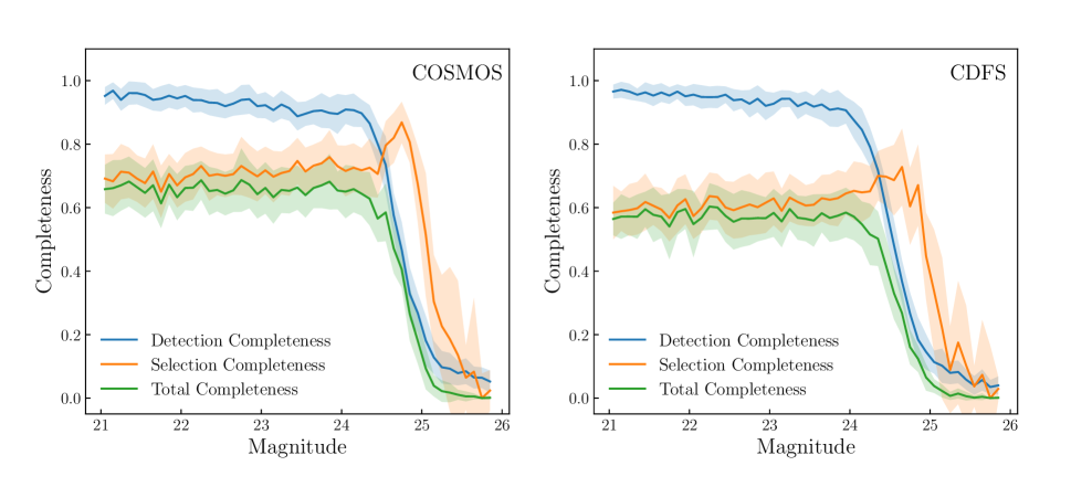
Figure 4.— The LAE sample completeness (total completeness; green line) as a function of input NB964 total magnitude derived through injection and recovery simulations. The detection completeness (blue line) plots the fraction of injected pseudo LAEs which can be detected in the corresponding narrowband image. The selection completeness (orange line) draws the fraction of NB964 detected pseudo LAEs which pass our LAE selection criteria. In each simulation trial we inject $\sim$ 3000 pseudo galaxies, and repeat 100 trials to estimate the average and 1$\sigma$ scatter (shaded regions) of the completeness measurements.

4. Ly$\alpha$ luminosity function

4.1. Sample incompleteness

It is essential to correct the sample incompleteness for the calculation of the luminosity function. Such incompleteness can be estimated through injection and recovery simulations, as described below.

We first run the Python package Balrog (Suchyta et al. 2016) which utilizes GALSIM (Rowe et al. 2015), to simulate pseudo LAEs, apply PSF convolution, and randomly insert the galaxies into the NB964 images. The pseudo galaxies have a Sérsic profile with a Sérsic index $n$ of 1.5 and half-light radius of 0.9 kpc , corresponding to 0.17″ at $z\sim 7$. The adopted Sérsic index and half-light radius are similar to the recent UV continuum profile measurements of high redshift LAE and LBG galaxies in the EoR (e.g., 0.5 – 0.7 kpc for narrowband selected LAEs, and 0.9 – 1.0 kpc for broadband selected LBGs, Jiang et al. 2013; Allen et al. 2017; Shibuya et al. 2019). The magnitudes of pseudo galaxies in the narrowband are randomly given in the range of 21 to 26. We then run SExtractor on the NB964 images after injections, with the identical configuration we used for detecting true LAEs.

Note the Ly$\alpha$ emission in LAEs could be more extended than the UV continuum (e.g. Finkelstein et al. 2011; Momose et al. 2016; Yang et al. 2017; Leclercq et al. 2017). For instance, with HST narrowband imaging data, Finkelstein et al. (2011) reported 3 $z\sim 4.4$ LAEs have an averaged Ly$\alpha$ emission half-light radius of 1.1 kpc, larger than that of the UV continuum (0.7 kpc). Leclercq et al. (2017) reported the detection of extended Ly$\alpha$ halos around $z\sim$ 3–6 LAEs, observed with the Multi-Unit Spectroscopic Explorer (MUSE) at ESO-VLT. Through two-component (continuum-like and halo) decomposition, they reported an exponential scale length of $3.8\pm 1.3$ kpc for the halo and $0.3\pm 0.1$ kpc for the core in their highest redshift bin ($z\sim$ 5–6). Directly taking their measured Ly$\alpha$ profiles, we calculate the effective half-light radius of the total Ly$\alpha$ emission (core plus halo) for each LAE, and find a medium value of 1.5 kpc at $z\sim$ 5–6. To address such effect, we also simulate pseudo LAEs with larger half-light radius of 1.2 kpc and 1.5 kpc, and find negligible difference in the completeness measurements. Thus, in this work, we adopt a half-light radius of 0.9 kpc to be consistent with previous works (e.g. Zheng et al. 2017; Konno et al. 2018).

We plot the fraction of the pseudo galaxies that are detected (with S/N $>$ 5 in both 2″ and 1.35″ aperture) as a function of magnitude in Fig. 4 (detection completeness hereafter). Though masking out the regions around the bright stellar halos and CCD artifacts is a common approach for LAE selection (e.g. Ota et al. 2017; Itoh et al. 2018), the detection completeness is still slightly less than unity even for the bright pseudo galaxies. This is because they might still blend with bright foreground sources, making them undetectable by SExtractor in NB964 images. The detection completeness gradually drops with decreasing pseudo galaxy brightness before reaching the limiting magnitudes, as blending with foreground galaxies could hinder their detections.

However, not all the NB964-detected pseudo LAEs passed our LAE selection criteria, since many of them were blended with foreground sources that were not bright enough to block them from NB964 detections, but sufficiently bright to make them fail the requirement of veto band non-detection and/or color-excess. We apply our LAE selection criteria on the NB964-detected pseudo galaxies, and plot the recovery fraction (relative to the number of NB964 detected pseudo objects, hereafter “selection completeness”) in Fig. 4. Note we insert the pseudo galaxies only into NB964 image and assume their underlying broadband fluxes to be zero. The effects if we insert also pseudo underlying broadband fluxes based on Ly$\alpha$ line EW are rather complicated (see Zheng et al. 2014). Basically, while high EW pseudo LAEs can be easily recovered by the selection procedure, some low EW sources could be missed by our selection due to photometric fluctuations. However, a contrary effect is that some pseudo LAEs with intrinsic line EWs below our EW limit could also have their line EWs boosted by photometric fluctuations, thus be picked up. The net effect is an Eddington type bias, and can be quantitatively estimated with an accurate EW distribution, which is yet unavailable at $z\sim$ 7.0. Nevertheless, as shown by Zheng et al. (2014) , such bias is rather weak, as long as the underlying broadband image is $>$ 0.5 – 1.0 mag deeper than the NB image, a condition that well satisfied by our datasets. Thus in this work we do not consider broadband fluxes of pseudo galaxies in the simulations.

Clearly, the effect of “selection incompleteness” is remarkable and shall not be neglected. Such incompleteness is mainly due to foreground contamination in the veto broadband photometry. The effect of blending with foreground sources in the veto band can also be roughly estimated with random aperture photometry. For example, only $74.9\%$ of the $1.35\arcsec$ randomly placed apertures in the COSMOS HSC-$g$ band image yield S/N $<3\sigma$. The fraction further decreases to $68.3\%$ and $59.6\%$ if the aperture diameter increases to 2″ and 3″, respectively. Therefore, deriving veto band photometry using larger aperture would yield stronger sample incompleteness due to foreground contaminations. The incompleteness is also sensitive to the depth and PSF of the veto broadband images, i.e., the foreground contamination to the veto broadband would be more severe for deeper images, or those with poorer PSF.

We further note that the “selection completeness” is not constant, but magnitude-dependent (Fig. 4). The “selection completeness” gradually increases with increasing magnitude. This is because a fainter pseudo LAE, if blended with foreground source(s), would more likely be treated as part of the adjacent object(s) and simply not detected in the narrowband image by SExtractor. Such effect, which is more important toward fainter magnitude, would suppress the detection completeness. Consequently, those non-detected pseudo LAEs would be pre-excluded from the calculation of “selection completeness”, which in turn gets boosted (as seen in Fig. 4). Near the detection limit where the detection completeness sharply drops, the effect is so strong that most of the detected pseudo LAEs are located in sparse regions, i.e., free from contaminations, and the selection completeness even exhibits a significant peak. Meanwhile the “selection completeness” significantly drops at faintest magnitudes, as most of the faintest pseudo LAEs could be detected solely because they were injected by coincidence on top of foreground sources.

The total sample completeness (the product of detection completeness and selection completeness, i.e, the fraction of injections that can be recovered as LAEs) is plotted in Fig. 4. We note that the “detection incompleteness” in the narrowband images has usually been corrected for the Ly$\alpha$ luminosity function reported in the literature. Unfortunately, the “selection incompleteness”, which is indeed more prominent as we demonstrated above, has not been considered in previous studies.

4.2. Ly$\alpha$ Luminosity Function at $z\sim 7$

Following Zheng et al. (2017), we calculate the $z\sim 7$ LAE luminosity function using the formula:

$$\Phi(L)dL=\sum_{L_{i}\in[L-\Delta L/2,L+\Delta L/2]}\frac{1}{V_{\mathrm{eff}}f_{\mathrm{comp}}(NB_{i})}dL,$$ (5)

where $V_{\mathrm{eff}}$ is the effective volume of the survey which is calculated from sky coverage and redshift coverage, and $f_{\mathrm{comp}}$ the completeness described in Section 4.1 for each LAE with NB964 magnitude $NB_{i}$. The effective volume is $1.29\times 10^{6}$ cMpc³ and $1.14\times 10^{6}$ cMpc³ for CDFS and COSMOS field, respectively, with bad regions, such as CCD artifacts and bright stellar halos, removed. We do not take the contamination into account, since we expect only a few foreground ELGs can be included in our LAE sample (see Sec. 3.3).

The resulting luminosity functions are plotted in Fig. 5. The bright end luminosity bump in COSMOS, first reported by Zheng et al. (2017), is confirmed with a doubly large sample size. A detailed comparison with the LF in Zheng et al. (2017) is presented in §4.3. We interpret the bump in COSMOS as an evidence of ionized bubbles at $z\sim 7$ (see Section 5.1). Remarkably, while the faint end luminosity functions from two field agree with each other, the bright end bump is not seen in CDFS.

Table 2Best-fit Schechter Parameters of Ly$\alpha$ luminosity function and Ly$\alpha$ luminosity density from $z\sim 5.7$ to $7.3$

$z$	Field	$L$ Fitted Range (erg s-1)	$\log_{10}L^{\ast}_{Ly\alpha}$ (erg s-1)	$\log_{10}\Phi^{\ast}$ (Mpc-3)	$\alpha$	$\log_{10}\rho_{Ly\alpha}$ (erg s-1 Mpc-3)	Transmission ($T^{IGM}_{z}/T^{IGM}_{5.7}$)
Selection incompleteness corrected
6.9	COSMOS	$42.65-43.4$	$42.75^{+0.15}_{-0.11}$	$-3.02^{+0.38}_{-0.44}$	$-2.5$(fixed)	$39.57\pm 0.13$
6.9	CDFS	$42.65-43.4$	$42.93^{+0.21}_{-0.13}$	$-3.62^{+0.37}_{-0.48}$	$-2.5$(fixed)	$39.38\pm 0.09$
6.9	COSMOS+CDFS	$42.65-43.65$	$42.94^{+0.11}_{-0.09}$	$-3.60^{+0.25}_{-0.28}$	$-2.5$(fixed)	$39.42\pm 0.08$
Selection incompleteness uncorrected
5.7a	HSC SSP	$42.4-44.0$	$43.21^{+0.36}_{-0.24}$	$-4.07^{+0.51}_{-0.28}$	$-2.56^{+0.53}_{-0.45}$	$39.54$	1
6.6a	HSC SSP	$42.4-44.0$	$43.22^{+0.07}_{-0.23}$	$-4.33^{+0.61}_{-1.27}$	$-2.49^{+0.50}_{-0.50}$	$39.26$	$0.70\pm 0.15$
6.9	CDFS+COSMOS	$42.65-43.65$	$43.08^{+0.14}_{-0.11}$	$-4.19^{+0.26}_{-0.31}$	$-2.5$(fixed)	$39.13\pm 0.07$	$0.63\pm 0.12$
7.3b	SXDS+COSMOS	$42.4-43.0$	$42.77^{+1.23}_{-0.34}$	$-4.09^{+1.09}_{-1.91}$	$-2.5$(fixed)	$38.55\pm 0.17$	$0.29\pm 0.19$

• ^a The LFs at $z\sim 5.7$ and $6.6$ are from Konno et al. (2018).

• ^b The best-fit Schechter parameters for LF at $z\sim 7.3$ when assuming a fixed slope of $\alpha=-2.5$ and using the data points from Konno et al. (2014).

We fit a Schechter function to the luminosity functions as:

$$\Phi(L)dL=\Phi^{\ast}\left(\frac{L}{L^{\ast}}\right)^{\alpha}\exp\left(-\frac{L}{L^{\ast}}\right)d\left(\frac{L}{L^{\ast}}\right),$$ (6)

where $L^{\ast}$ and $\Phi^{\ast}$ are the characteristic luminosity and number density, respectively. We fix the faint end LF slope $\alpha$ of the Schechter function to $-2.5$, consistent to those observed at $z\sim 5.7$ and $6.6$ (e.g. Konno et al. 2018; Santos et al. 2016; Matthee et al. 2015). The three LAEs in the lowest luminosity bin in COSMOS have selection completeness $f_{comp}$ (see equation 5) $<$ 0.1. This indicates this luminosity bin suffers from incompleteness too strong to be accurately estimated and corrected, and thus we exclude it from further analyses. In Fig. 5 we fit the luminosity functions from both fields in the luminosity range of 10^42.65 – 10^43.4 erg s^-1, i.e., excluding the two brightest luminosity bins for COSMOS as there are no LAEs in CDFS in these two bins. We use the Cash Statistics (a maximum likelihood-based statistics for Poisson data, i.e., low number of counts, Cash 1979) to estimate the best-fit value and error of $L^{\ast}$ and $\Phi^{\ast}$. The best-fit curves are plotted in the Fig. 5 and the best-fit Schechter parameters are listed in Tab. 2. To better illustrate the bright end bump in COSMOS, we plot the Schechter function elevated and truncated at the bright end to match the two brightest bins.

We also present the LF averaged over two fields in the middle panel of Fig. 5, together with the best-fit Schechter function (over the full luminosity range of 10^42.64 – 10^43.65 erg s^-1). For comparison, we over-plot the “selection incompleteness” uncorrected LF, e.g., with only “detection incompleteness” corrected. Leaving the “selection incompleteness” uncorrected clearly yields underestimated LF. The z $\sim$ 7.0 LFs from Itoh et al. (2018) and Ota et al. (2017) are also over-plotted, in both of which the “selection incompleteness” correction was unavailable thus not applied.

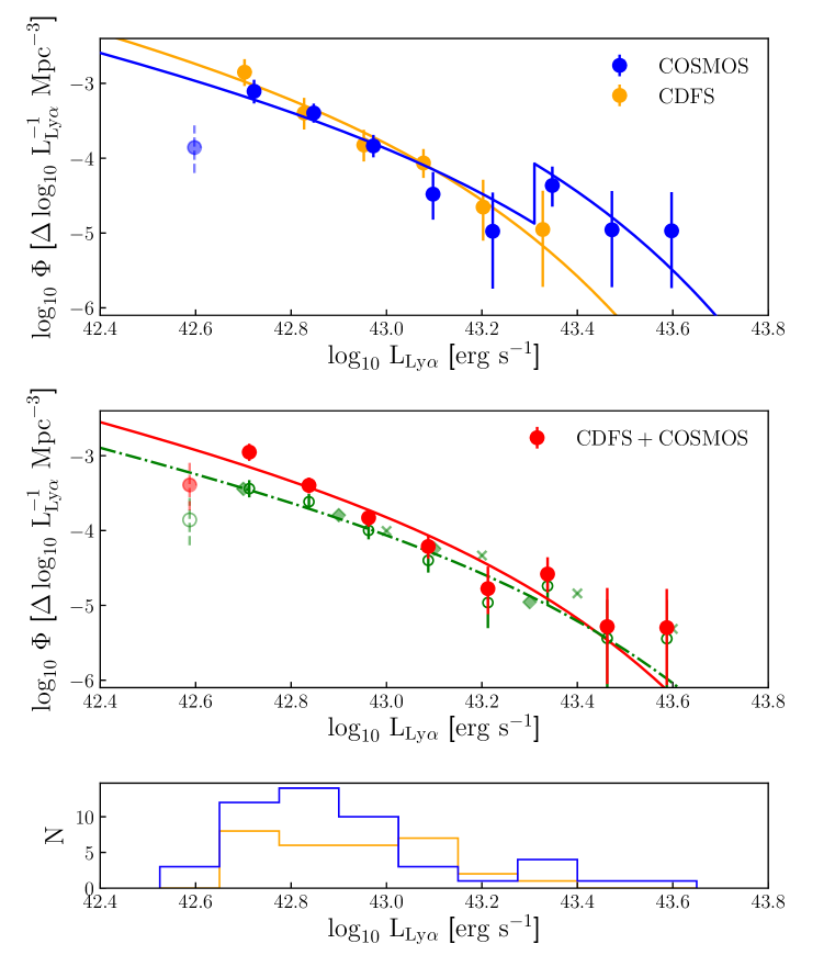
Figure 5.— Ly$\alpha$ LFs for our LAEs (selection incompleteness corrected). Upper panel: the LFs from COSMOS and CDFS separately. To avoid confusion, the data points were horizontal shifted by $+0.01$ and $-0.01$ dex for COSMOS and CDFS respectively. A clear bright end bump is seen in COSMOS but not in CDFS. Middle panel: the LF averaged over two fields (red). To illustrate the effect of “selection incompleteness”, we over-plot the “selection incompleteness” uncorrected LF of this work in green open circles and green dot-dashed line. We also over-plot the data points of $z\sim$ 7.0 LAE LFs from Ota et al. (2017) and Itoh et al. (2018) in green diamonds and green crosses, respectively, in both of which the “selection incompleteness” was not corrected. The left most LF bin (semi-transparent data points) in both the top and middle panels suffer strong incompleteness, and were excluded from further analyses. In both panels, the best-fit Schechter functions with $\alpha=-2.5$ are over-plotted (see text for details). Lower panel: the number of LAEs in each field in each luminosity bin.

4.3. The Effect of the Underlying Broadband Depth

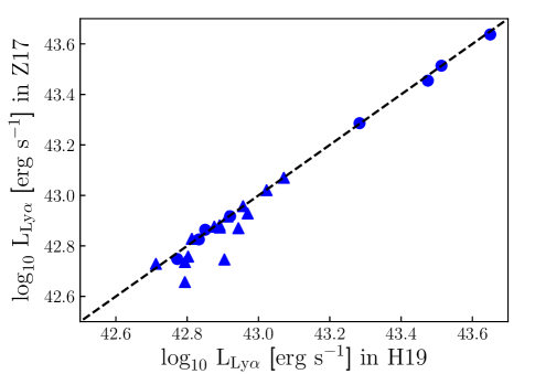
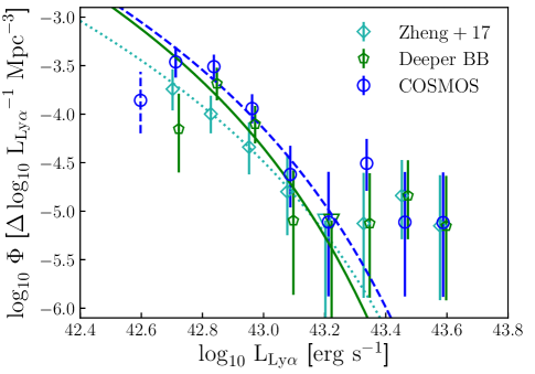
Figure 6.— Upper panel: The Ly$\alpha$ line luminosities for the 23 LAEs selected by Zheng et al. (2017), recalculated with the much deeper underlying HSC-$y$ photometry in this work (x-axis), versus those calculated with the shallower UltraVISTA Y band photometry (y-axis). The triangles plot the sources non-detected in the underlying broadband in Z17. Lower Panel: Comparing the COSMOS field Ly$\alpha$ LF obtained in this work (blue circles) with that from Zheng et al. (2017, cyan diamonds). The green pentagons plot the recalculated LF based on the LAE sample of Zheng et al. (2017) but with much deeper underlying broadband photometry (HSC-$y$ band). To be consistent with Zheng et al. (2017), we fit the Schechter function to the data points within $L$ range $42.65\leqslant\log_{10}L\leqslant 43.25$ in this figure.

In Fig. 6 we compare the Ly$\alpha$ luminosity function in COSMOS obtained in this work with that reported in Zheng et al. (2017). To enable a direct comparison, the selection incompleteness described in §4.1 is ignored in this plot, as it was uncorrected in Zheng et al. (2017). While at the highest luminosity bins both luminosity functions appear consistent, the new luminosity function obtained in this work is considerably higher at fainter luminosity bins. However, this is only partly due to the fact that we select more candidates in this work.

Another and dominant reason is the depth of the underlying broadband image. As described in Section 3.1, for a LAE candidate which is not detected in the underlying broadband, a widely used approach is to place a 2$\sigma$ upper limit to its broadband flux density and use such upper limit and narrowband flux density to estimate the Ly$\alpha$ flux. As we demonstrate below, this step would yield significantly under-estimated Ly$\alpha$ flux and bias the LF if the underlying broadband is not sufficiently deep. Zheng et al. (2017) adopted NB964 and the UltraVISTA $Y$ band image to calculate the Ly$\alpha$ fluxes. For most of the faint candidates, UltraVISTA Y band detections are not available and 2$\sigma$ upper limits were given to their BB fluxes. In this work, the underlying broadband in COSMOS is HSC-$y$, which is considerably deeper than UltraVISTA $Y$ (by $\sim$ 1.1 – 2.5 mag, as the depth of UltraVISTA $Y$ is not uniform). To simply illustrate such effect, we re-calculate the Ly$\alpha$ line luminosity and the luminosity function of 23 LAE candidates selected by Zheng et al. (2017) with old NB964 photometry but new HSC-$y$ photometry. For sources which are not detected in HSC-$y$, we adopt the 2$\sigma$ limiting magnitude of HSC-$y$. The comparison of the resulted Ly$\alpha$ luminosities is given in the upper panel of Fig. 6, where we see that for a significant fraction of faint LAEs, the Ly$\alpha$ luminosities had been under-estimated with shallower underlying broadband photometry. As shown in the Fig. 6, the deeper underlying broadband could significantly elevate the faint end LF to a level more consistent with this work. The bright end LF does not change much because most of the luminous LAEs were already detected in UltraVISTA $Y$.

With simulations, Zheng et al. (2014) showed that the depth of the underlying broadband could significantly affect the LAE selection, and a broadband image $\sim$ 0.5 – 1.0 mag deeper than the narrowband is most efficient in selecting emission line sources. In this work, we show an additional effect of the underlying broadband depth, which would affect the calculation of line flux and thus LF. This effect could be particularly significant for faint LAEs with large line equivalent width, for which we expect very weak underlying broadband signal, and whose line flux measurements would be obviously biased by an upper limit from the BB if it is not sufficiently deep. To estimate the required BB depth which would eliminate this bias, we assume an extreme case with Ly$\alpha$ line only. The line signal is detected in the narrowband with S/N $>$ 5, and we expect to detect it in the BB with S/N $>$ 2. The underlying broadband is thus required to be $2.5\log(W_{BB}/W_{NB})-2.5\log(5/2)$ deeper than the inside narrowband, where $W_{NB}$ and $W_{BB}$ are the width of the narrow- and broadband filters. Practically, LAEs have finite line EW, thus we expect continuum signal in both narrowband and the underlying broadband, and BB $\sim$ 1.0 – 1.5 mag deeper than the NB would be sufficient, depending on the bandpass of the filters. The underlying broadbands adopted in this work are indeed sufficiently deep, and the luminosity functions we obtained are free from significant bias.

5. Discussion

5.1. The Bright End Bump in the Ly$\alpha$ Luminosity Function at $z\sim 7.0$

Zheng et al. (2017) firstly detected a bright end bump in the LF of $z\sim 7.0$ LAEs in COSMOS field with four luminous LAEs (L_Lyα $>10^{43.3}$ erg s^-1). This suggests the existence of ionized bubbles at $z\sim 7$ which reduce the opacity of neutral IGM around the luminous LAEs (see §4.3 in Zheng et al. 2017). Such a bright end LF bump is confirmed in this work, with six luminous LAEs (L_Lyα $>$ 10^43.3 erg s^-1) selected in COSMOS field. One of the newly selected luminous LAE did not pass the selection in Zheng et al. (2017) because it is close to a nearby bright source and its 2″ aperture veto band photometry is significantly contaminated. It is selected in this work as we adopt a 1.35″ aperture in our veto band photometry. Another newly selected luminous LAE was classified as a possible foreground source in Zheng et al. (2017) due to visually identified marginal signal in one of the previously adopted veto bands. With the deeper HSC ultra deep images used in this work (also with better seeing), we did not reveal any signal in any of the new veto bands. The marginal signal in the old veto band is indeed due to data processing flaw, and was confirmed to be artificial with improved reprocessing of the old veto band images.

Strikingly, while the faint end LF from a second LAGER field CDFS is quite consistent with that from COSMOS, the bright end LF bump is not seen in CDFS, in which only one luminous LAE is selected. Such field-to-field variation in the bright end LF is also visible when comparing with other $z\sim 7.0$ LAE samples in literature. Ota et al. (2017) identified 20 $z\sim 7.0$ LAE candidates using Subaru Suprime-Cam and NB973_SSC filter. The sample was selected in a smaller volume (0.61$\times$10⁶ Mpc³) with no LAEs with L_Lyα $>$ 10^43.3 erg s^-1. Itoh et al. (2018) identified 34 $z\sim 7.0$ LAE candidates using Subaru HSC and NB973_HSC filter in two fields (COSMOS: 1.15$\times$10⁶ Mpc³, SXDS: 1.04$\times$10⁶ Mpc³). While Itoh et al. (2018) claimed no evidence of bright end LF bump, they did identify 4 luminous LAEs in COSMOS, but zero in SXDS. Such field-to-field variation is similar to what we see in the two LAGER fields. Additional reasons that Itoh et al. (2018) did not detect the bright end LF bump include that: 1) Itoh et al. (2018) adopted larger luminosity bins in their LFs (0.2 dex comparing with 0.125 dex adopted in this work and Zheng et al. 2017); 2) the NB973_HSC filter that Itoh et al. (2018) used has Gaussian-like transmission curve with clear wings (Itoh et al. 2018), while the transmission curve of our NB964 filter is more box-car shaped (see Zheng et al. 2019 and Fig. 1). A Gaussian-like transmission curve would yield large uncertainties in the Ly$\alpha$ luminosity derived from narrowband photometry, and would significantly underestimate the luminosity and number of LAEs whose Ly$\alpha$ lines fall on the wings of the bandpass. Such large uncertainties could likely smear out the bump feature in the LF.

As the bandpass of NB973_HSC and our NB964 overlap (Zheng et al. 2019), we compare our LAEs with that of Itoh et al. (2018) in COSMOS and find 7 common LAEs selected by both programs. Particularly 3 out of the 4 luminous LAEs selected by Itoh et al. (2018) are included in our sample. Two of them (HSC-z7LAE3 and HSC-z7LAE25) were classified as luminous LAEs by Itoh et al. (2018), but only after they recalibrated their Ly$\alpha$ luminosities using our spectroscopic redshifts (Hu et al. 2017), i.e., they fall on the NB973_HSC transmission curve wing. We select another (HSC-z7LAE2) that coincides with the core of one LAE-overdense region in Fig. 3, but its NB964-based Ly$\alpha$ luminosity (10^42.7 erg s^-1) is considerably lower than 10^43.4 from Itoh et al. (2018). The last luminous LAE (HSC-z7LAE1) selected by Itoh et al. (2018) is also significantly detected in our NB964 image. This source, however, did not pass our selection due to foreground contamination in the veto bands. After excluding the contamination, the NB964-derived Ly$\alpha$ luminosity of HSC-z7LAE1 is 10^43.0 erg s^-1, also considerably lower than 10^43.5 from Itoh et al. (2018). Both HSC-z7LAE1 and HSC-z7LAE2 might fall on the transmission curve wing of our NB964 filter, i.e., have underestimated NB964-based Ly$\alpha$ luminosity.

If HSC-z7LAE1 and HSC-z7LAE2 are included as luminous LAEs in our sample, the number of luminous LAEs selected in LAGER COSMOS rises to 8, further strengthening the robustness of the bright end LF bump and the field-to-field variation. We also stress that the three luminous LAEs in COSMOS field and the single luminous LAE in CDFS have been spectroscopically confirmed (Hu et al. 2017; Yang et al. 2019). Meanwhile, as shown in Fig. 7, our new Ly$\alpha$ LF at $z\sim 7.0$, averaged over two LAGER fields, is well consistent from those from Ota et al. (2017) and Itoh et al. (2018).

All 6 luminous LAEs are located within the two large scale structures (Fig. 3). This indicates that large ionized bubbles at $z\sim$ 7.0 are closely associated with cosmic overdensities. Note that two $z\sim 7$ LAEs with projected distance of $\sim 90$ pkpc are confirmed by Castellano et al. (2018), which are also selected in an overdense region identified with several Lyman Break Galaxy (LBG) candidates (Castellano et al. 2016). These provide direct observational supports to the inside-out reionization topology (e.g. Iliev et al. 2006; Choudhury et al. 2009; Friedrich et al. 2011). Further clustering analysis and follow-up observations of the overdense regions in COSMOS are essential to study the patchy reionization. The clear field-to-field variation of the bright end LF manifests the need of LAE searches in even more fields to probe the reionization and large scale structures in the early universe.

5.2. Evolution of Ly$\alpha$ Luminosity Function and Constraint to Neutral Hydrogen Fraction

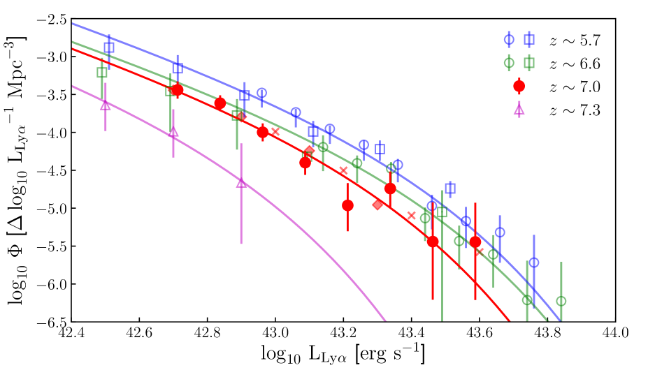
Figure 7.— Evolution of Ly$\alpha$ LFs from $z\sim 5.7$ to $7.3$. The red filled circles are the LF of our $z\sim 7.0$ LAEs and the red solid line is best-fit Schechter function. The $z\sim 7.0$ LFs from Itoh et al. (2018) and Ota et al. (2017) are plotted with red crosses and diamonds respectively, which agrees well with ours. The blue squares and circles are the Ly$\alpha$ LFs at $z\sim 5.7$ from Ouchi et al. (2008) and Konno et al. (2018), respectively. The green opened squares and circles are the Ly$\alpha$ LFs at $z\sim 6.6$ from Ouchi et al. (2010) and Konno et al. (2018), respectively. The purple opened triangle are the Ly$\alpha$ LF at $z\sim 7.3$ from Konno et al. (2014). The blue, green and purple solid lines are the corresponding best-fit Schechter function from $z\sim 5.7$, $6.6$, $7.3$ LFs.

In Fig. 7, we plot our Ly$\alpha$ LF (averaged over two LAGER fields) at $z\sim$ 7.0 together with those at $z\sim 5.7$ to $7.3$ (Ouchi et al. 2008, 2010; Konno et al. 2014, 2018). We stress that the “selection incompleteness” described in §4.1 was not corrected in this plot, as such incompleteness was not available for LFs given in literature. We assume those LAE samples at redshift 5.7 – 7.3 suffer from similar “selection incompleteness” when we compare the uncorrected LFs to demonstrate cosmic evolution in the luminosity function. A gradual evolution between redshift of 5.7 and 7.3 is clearly seen in Fig. 7. Note the LF at $z\sim$ 7.3 is based on a rather small photometric sample (7 LAEs, Konno et al. 2014), thus the error bars are considerably larger. To further quantify the evolution of LFs from $z\sim 5.7$ to $7.3$, we plot the contours of best-fit Schechter function parameters (L^∗ and $\phi^{*}$) for LFs at $z\sim 5.7$, $6.6$, $7.0$, and $7.3$ in Fig. 8. In this plot, for our LF at $z\sim$ 7.0, we plot both “selection incompleteness” corrected (dashed red) and uncorrected (solid red) results to illustrate the effect of such incompleteness correction.

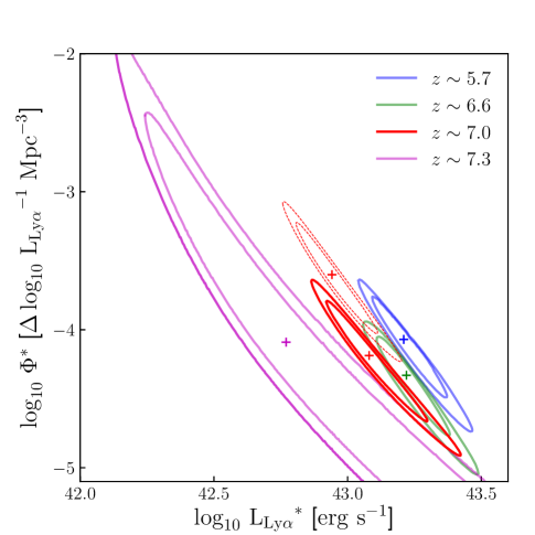
Figure 8.— $68\%$ and $90\%$ Confidence intervals of the best-fit Schechter parameters L^∗ and $\Phi^{\ast}$ for our $z\sim 7.0$ LF from two LAGER fields (solid red: uncorrected “selection incompleteness”). The “selection incompleteness” corrected version is plotted with dashed red lines to illustrate the effect of such incompleteness. We also plot the confidence interval of best-fit Schechter parameters of LFs (all with uncorrected “selection incompleteness”) at $z\sim 5.7$, $6.6$ (Konno et al. 2018), and $7.3$ (Konno et al. 2014)

The luminosity density of Ly$\alpha$ photons is derived by integrating our Ly$\alpha$ LF in the luminosity range of $\log\mathrm{L_{Ly\alpha}}$ [erg s^-1] $=42.4-44$. The evolution of Ly$\alpha$ luminosity density from $z\sim 5.7$ to $7.3$ are plotted in the Fig. 9. We also plot the UV luminosity density from Finkelstein et al. (2015), based on the galaxy LFs from $z\sim 4$ – $8$ using galaxies selected by photometric redshift with Hubble Space Telescope (HST) imaging data.

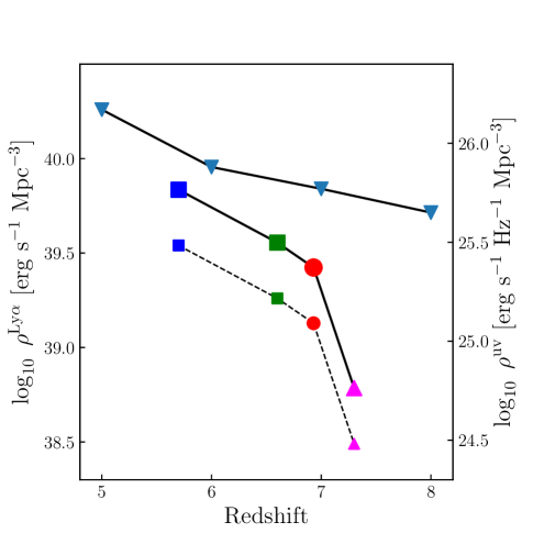
Figure 9.— Evolution of Ly$\alpha$ luminosity density (dashed line, uncorrected for sample selection incompleteness) from $z\sim 5.7$ to $7.3$. The Ly$\alpha$ luminosity density at $z\sim 5.7$ and $6.6$ are from Konno et al. (2018) and the Ly$\alpha$ luminosity density at $z\sim 7.3$ are from Konno et al. (2014). We also plot the evolution of UV luminosity density (inverse triangles) derived by Finkelstein et al. (2015). The larger symbols and the solid line for Ly$\alpha$ luminosity density are corrected for LAE sample “selection incompleteness”, assuming a common correction factor of 0.3 dex as we derived for our $z\sim$ 7.0 LAE sample.

Below we estimate the effective IGM transmission factor $T^{IGM}_{z}$ and neutral hydrogen fraction $\chi_{HI}$ following Ouchi et al. (2010). The observed Ly$\alpha$ luminosity density can be simply converted from UV luminosity density:

$$\rho^{Ly\alpha}=\kappa T^{IGM}f_{esc}\rho^{UV},$$ (7)

where $\kappa$ is the conversion factor from UV photons to Ly$\alpha$ photons; $f_{esc}$ the Ly$\alpha$ escape fraction through the ISM (Dijkstra et al. 2007a; Dijkstra & Wyithe 2010; Cai et al. 2014; Dayal & Ferrara 2018); and $T^{IGM}$ the transmission of the IGM. Assuming the properties of ISM and stellar population are the same at $z=5.7$ and $7.0$, the IGM transmission at $z\sim 7.0$ can be calculated:

$$\frac{T^{IGM}_{7.0}}{T^{IGM}_{5.7}}=\frac{\rho^{Ly\alpha}_{7.0}/\rho^{Ly\alpha}_{5.7}}{\rho^{UV}_{7.0}/\rho^{UV}_{5.7}}.$$ (8)

We linearly interpolate the UV luminosity density in Fig. 9 (Finkelstein et al. 2015) and estimate ${\rho^{UV}_{7.0}/\rho^{UV}_{5.7}}=0.63\pm 0.09.$ We then obtain $T^{IGM}_{7.0}/T^{IGM}_{5.7}=0.63\pm 0.12$ with Eq. 8, which indicates statistically significant evolution in the IGM suppression to the Ly$\alpha$ line.

It is model dependent to estimate the neutral hydrogen fraction $\chi_{\mathrm{HI}}$ based on the evolution of $T^{IGM}$. Below we present $\chi_{HI}$ inferred with several theoretical models.

With an analytical approach, Santos (2004) calculated the Ly$\alpha$ emission transmission through IGM as a function of neutral hydrogen fraction $\chi_{HI}$ in the early universe, considering the effects of IGM dynamics and galactic winds. Though the Ly$\alpha$ transmission through the IGM is highly sensitive to the Ly$\alpha$ line velocity offset, we can estimate the IGM neutral hydrogen fraction by comparing the observed $T^{IGM}_{7.0}/T^{IGM}_{5.7}$ with Fig. 25 of Santos (2004) while assuming no evolution in the Ly$\alpha$ line velocity offset between redshift 5.7 and 7.0. By doing so, we estimate a neutral hydrogen fraction of 0.25 – 0.50 for a galactic wind model with Ly$\alpha$ velocity offset of 360 km/s, and 0.30 – 0.50 for the case of no Ly$\alpha$ velocity shift.

Secondly, the observed evolution of Ly$\alpha$ LF can also be compared with radiative transfer simulations to constrain the reionization. McQuinn et al. (2007) calculated the effect of reionization on Ly$\alpha$ LF at $z=6.6$ with 200-Mpc radiative transfer simulations. The expected suppression to Ly$\alpha$ LF is given in Fig. 5 of McQuinn et al. (2007) for various global IGM neutral hydrogen fraction. Comparing our observations with the simulation results, we obtain similar constraints to $\chi_{\mathrm{HI}}$ (0.2 – 0.4).

We also compare our observations with the analytical calculations of Dijkstra et al. (2007b) and Furlanetto et al. (2006), which assume complete neutral IGM outside of ionized bubbles. Consistent with previous estimations, our observed $T^{IGM}_{7.0}/T^{IGM}_{5.7}$ corresponds to a globally averaged $0.2<\chi_{\mathrm{HI}}<0.5$.

6. Conclusion

Narrowband imaging surveys are powerful approaches to search for high redshift Ly$\alpha$ emitting galaxies and probe the cosmic reionization. We deploy a large area survey for $z\sim$ 7.0 LAEs (Lyman Alpha Galaxies in the Epoch of Reionization, abbr. LAGER) with a custom made narrowband filter installed on DECam onboard CTIO 4m Blanco telescope. In this paper, we present LAEs selected in the ultradeep LAGER-COSMOS field and a second deep field LAGER-CDFS. We present the Ly$\alpha$ luminosity function at $z\sim$ 7.0 and new knowledge inferred about cosmic reionization. Our major results are listed below:

1. We accumulate 47.25 hrs DECam NB964 exposure in COSMOS and 32.9 hrs in CDFS field. We select 49 $z\sim$ 7.0 LAEs in COSMOS and 30 in CDFS, building a largest ever LAE sample at $z\sim$ 7.0.

2. We find obvious LAE sample incompleteness due to foreground contamination in bluer veto broadband photometry. Such selection incompleteness (30% – 40% in this work), depending on the confusion level of the broadband images (seeing and depth), could cause underestimation of the luminosity function of high redshift galaxies, and thus should be carefully corrected.

3. We show that while calculating the Ly$\alpha$ luminosity based on narrow- and underlying broadband photometry, placing an upper limit to the broadband flux for non-detection might significantly bias the calculation of Ly$\alpha$ flux and luminosity function, if the broadband image is not sufficiently deep. We recommend the underlying BB be $\sim$ 1.0 – 1.5 mag deeper than the NB to avoid such bias.

4. Six luminous LAEs with L_Lyα $>$ 10^43.3 erg s^-1 constitute a bright end bump in the luminosity function in COSMOS, supporting the patch reionization scenario. The bump is however not seen in CDFS in which only one luminous LAE is selected. Except for the bright end bump, the luminosity functions from two fields agree with each other, and with those at $z\sim$ 7.0 in literature.

5. Two clear LAE overdense regions are detected in COSMOS, making them the highest redshift protoclusters observed to date. All six luminous LAEs in COSMOS fall in the overdense regions, further supporting the inside-out reionization topology.

6. We compare the LAGER LAE luminosity function at $z\sim$ 7.0 with those at $z\sim$ 5.7, 6.6, and 7.3 reported in literature, assuming they suffer similar “selection incompleteness”. We infer an average neutral hydrogen fraction of $\chi_{\mathrm{HI}}=0.2-0.4$ at $z\sim$ 7.0.

Appendix A A: On the color measurement

We examine the reliability of using SExtractor AUTO magnitudes to measure the narrowband to broadband color of LAEs, utilizing the injection and recovery simulations we introduced in §4.1. We use COSMOS field to present our analyses and results.

Following §4.1, we insert pseudo LAEs into the narrowband using a profile with Sérsic index of 1.5 and half-light radius of 0.9 kpc. We also insert corresponding signals into the underlying broadband HSC-$y$ (assuming an intrinsic color excess of 1 mag) using identical source profile. In the upper panel of Fig. 10, we plot the peak value and 1$\sigma$ scatter (measured through fitting the distribution with a Gaussian) of the output colors, as a function of the detected narrowband magnitude. We find while the AUTO-color could precisely recover the input value at the bright end, it slightly underestimate the color at the faint end. Meanwhile, the commonly used aperture color (using magnitudes measured on PSF-matched images within a fixed 2″ aperture, e.g., Ouchi et al. 2010; Ota et al. 2017), though also underestimates the color at the faint end, behaves slightly better.

The color underestimation at the faint end is mainly due to contamination from foreground sources to the pseudo LAE photometry in the narrow and broadband, i.e., as most foreground sources show no color excess, the contamination to the broadband photometry is relatively more prominent than to the narrowband. As our AUTO magnitudes are generally measured in regions larger than a 2″ aperture, the contamination effect is stronger for AUTO-color. In the middle panel of Fig. 10, we exclude pseudo LAEs with S/N $>$ 2 in any veto band to minimize the effect of contamination. We then see negligible difference between two approaches, and both could reliably measure the input color at all magnitudes (though the AUTO-color shows slightly larger scatter). Since we need to exclude sources with foreground contaminations anyway, both approaches are similarly reliable from this respect.

However, it is known that the Ly$\alpha$ emission in LAEs at lower redshifts is more extended than the UV continuum (e.g. Momose et al. 2016; Yang et al. 2017; Leclercq et al. 2017). In this case the aperture-color would underestimate the intrinsic value of LAEs. To depict such effect, we perform injections adopting slightly larger Ly$\alpha$ emission size (1.2 kpc half-light radius in the narrowband, and 0.9 kpc in the broadband). The recovered color is presented in the lower panel of Fig. 10, in which we see that, in case of more extended Ly$\alpha$ emission, the AUTO-color behaves better than aperture-color, especially at the bright end. Note the sizes and the Sérsic profiles here are adopted for illustration only. For instance, the half-light radius of 1.2 kpc we adopted is smaller than the typical size of the Ly$\alpha$ profile measured by Leclercq et al. (2017) at lower redshifts (see also §4.1). That is, if the Ly$\alpha$ spatial profile of $z\sim$ 7.0 LAEs is similar to that seen at lower redshifts, the effect will be even more significant than the modest case we illustrate above.

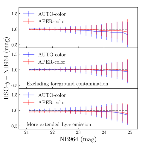
Figure 10.— The HSC-$y-\mathrm{NB964}$ color for simulated pseudo LAEs as a function of detected NB964 magnitude. Upper panel: the recovered color for narrowband detected pseudo LAEs; Middle panel: for detected LAEs without foreground contamination in veto bands (S/N $<$ 2 in veto bands). In the upper and middle panel, the injected sources have identical Sérsic profile (with half-light radius of 0.9 kpc) in both the NB964 image and HSC-$y$ image. Lower panel: similar to the middle panel but the injected sources have slightly larger size in the narrowband (with half-light radius of 1.2 kpc in NB964 and 0.9 kpc in HSC-$y$. The grey dashed lines indicate the input color.

Appendix B B: Thumbnail Images of our LAE Candidates

We show the thumbnail images of our LAE candidates in COSMOS and CDFS field in Fig. 11. We plot the veto broadband images, stacked veto broadband images (hereafter BB in the Fig. 11), NB964 images and underlying broadband images for each LAE candidates.

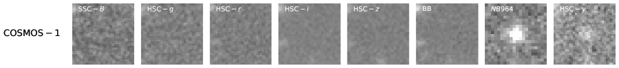
(a)

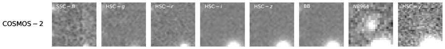
(b)

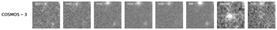
(c)

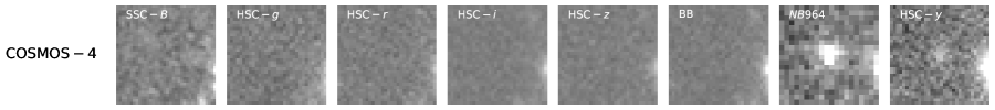
(d)

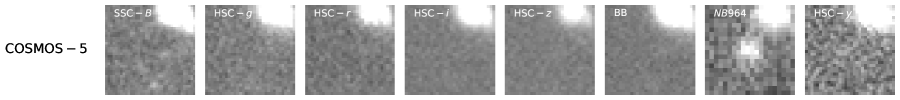
(e)

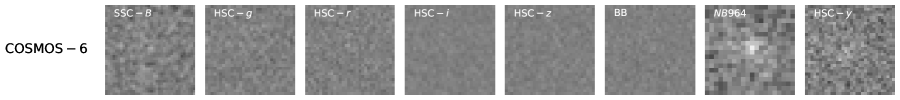
(f)

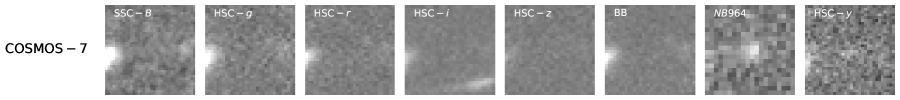
(g)

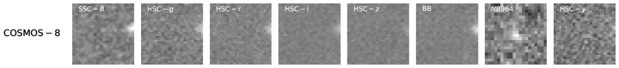
(h)

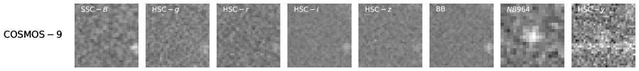
(i)

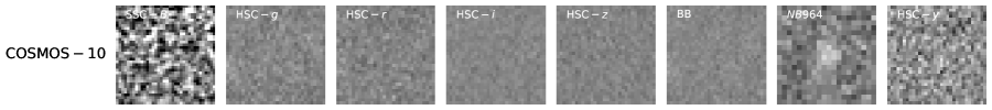
(j)

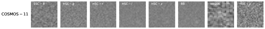
(k)

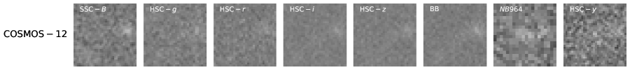
(l)

Figure 11.— The veto broadband images, stacked veto broadband images (namely BB), NB964 images and the underlying broadband images for LAE candidates in the COSMOS and CDFS field. The size of each image is $\sim 5.4\arcsec\times 5.4\arcsec$. The images are sorted by NB964 AUTO magnitude. Note the broadband images from HSC plotted here were before resampling (for illustration only).

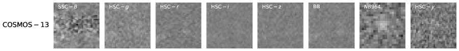
(m)

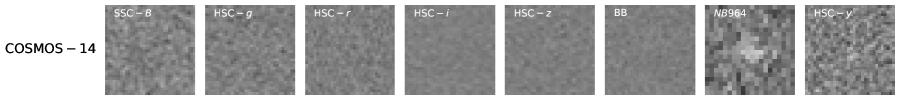
(n)

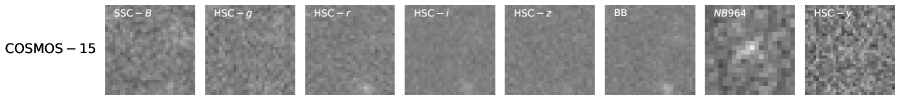
(o)

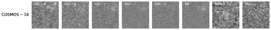
(p)

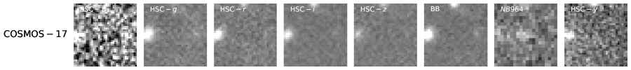
(q)

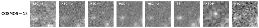
(r)

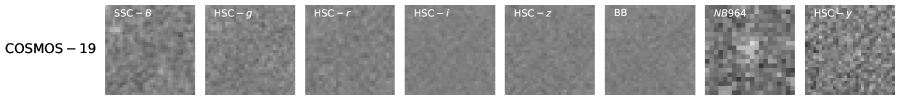
(s)

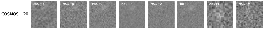
(t)

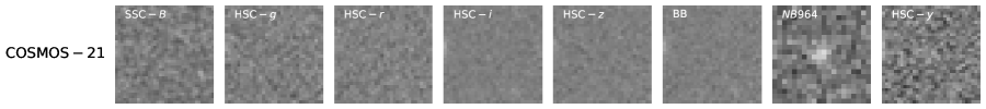
(u)

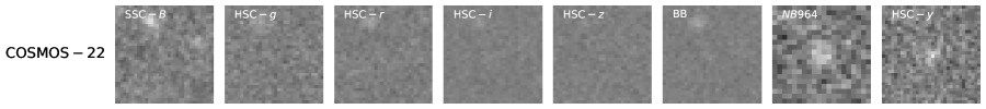
(v)

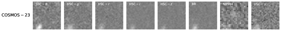
(w)

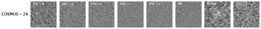
(x)

Figure 11.— Continued

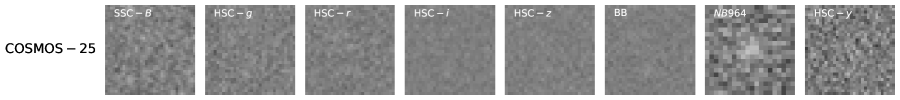
(y)

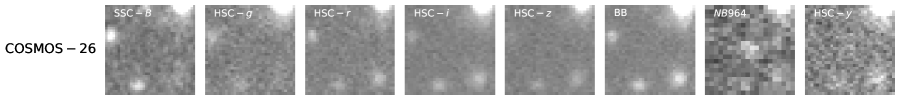
(z)

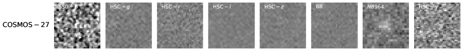
(aa)

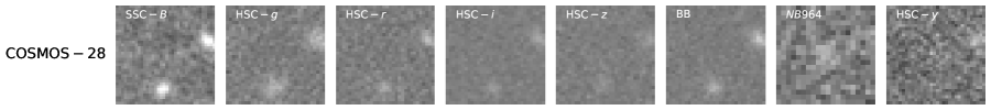
(ab)

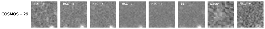
(ac)

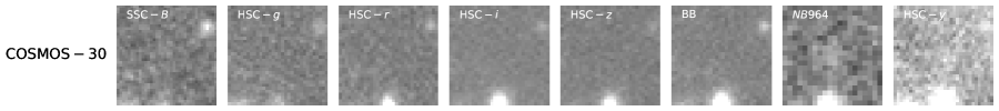
(ad)

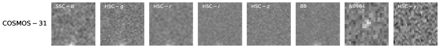
(ae)

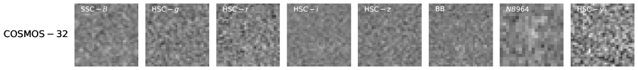
(af)

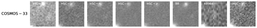
(ag)

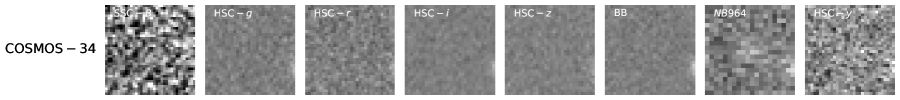
(ah)

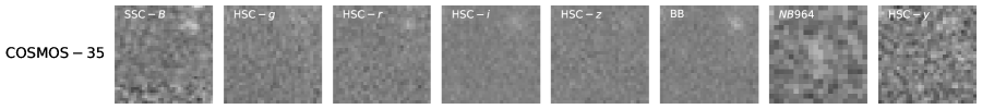
(ai)

(aj)

Figure 11.— Continued.

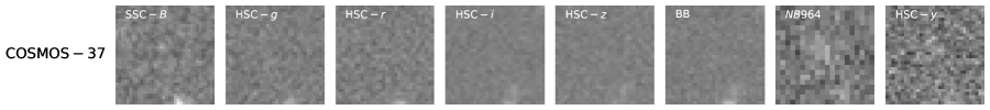
(ak)

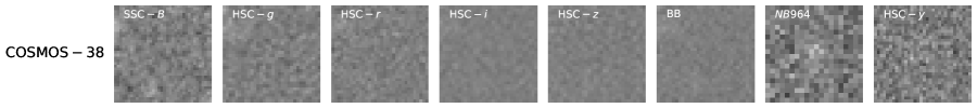
(al)

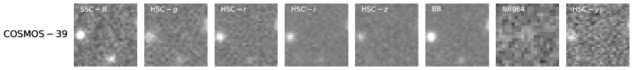
(am)

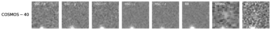
(an)

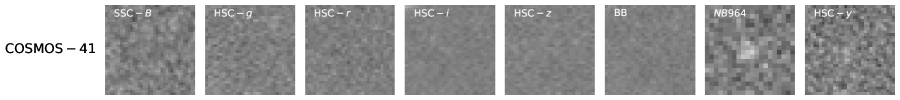
(ao)

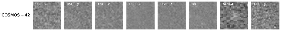
(ap)

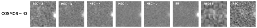
(aq)

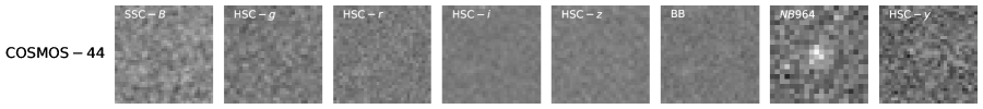
(ar)

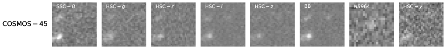
(as)

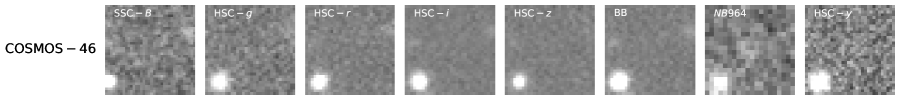
(at)

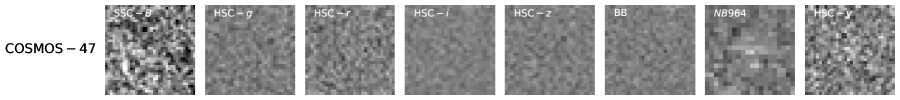
(au)

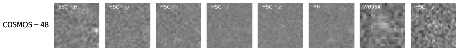
(av)

Figure 11.— Continued.

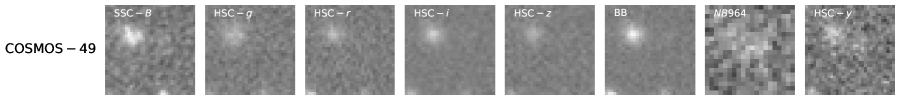
(aw)

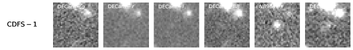
(ax)

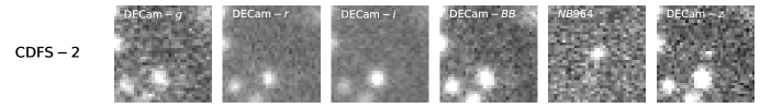
(ay)

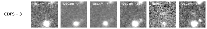
(az)

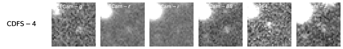
(ba)

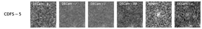
(bb)

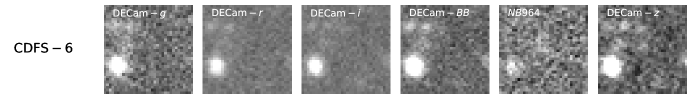
(bc)

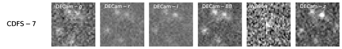
(bd)

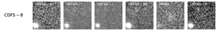
(be)

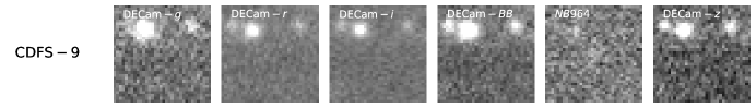
(bf)

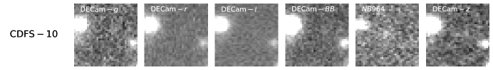
(bg)

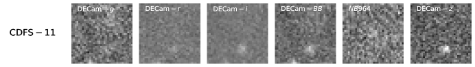
(bh)

Figure 11.— Continued.

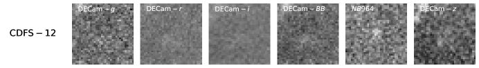
(bi)

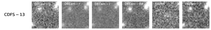
(bj)

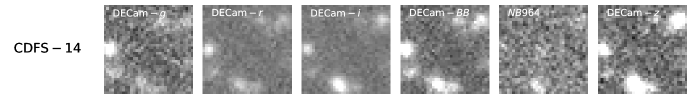
(bk)

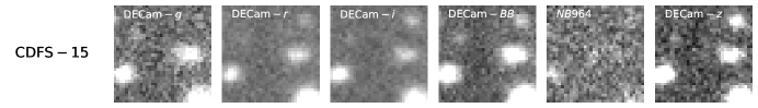
(bl)

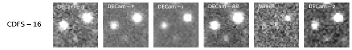
(bm)

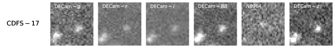
(bn)

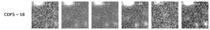
(bo)

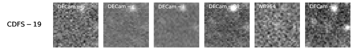
(bp)

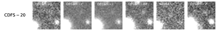
(bq)

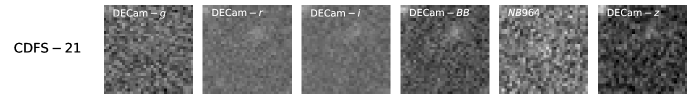
(br)

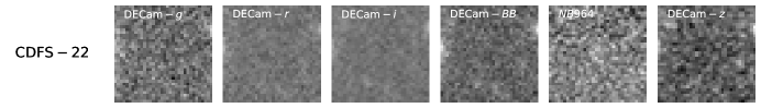
(bs)

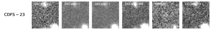
(bt)

Figure 11.— Continued.

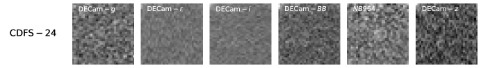
(bu)

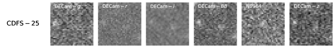
(bv)

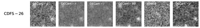
(bw)

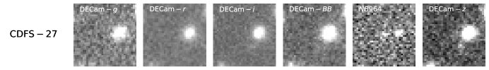
(bx)

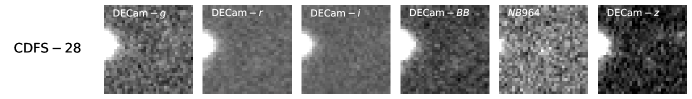
(by)

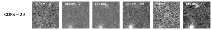
(bz)

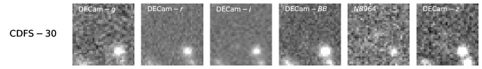
(ca)

Figure 11.— Continued.

References

- Abbott et al. (2018) Abbott, T. M. C., Abdalla, F. B., Allam, S., et al. 2018, ApJS, 239, 18
- Aihara et al. (2018) Aihara, H., Armstrong, R., Bickerton, S., et al. 2018, PASJ, 70, S8
- Allen et al. (2017) Allen, R. J., Kacprzak, G. G., Glazebrook, K., et al. 2017, ApJ, 834, L11
- Annis et al. (2014) Annis, J., Soares-Santos, M., Strauss, M. A., et al. 2014, ApJ, 794, 120
- Bañados et al. (2018) Bañados, E., Venemans, B. P., Mazzucchelli, C., et al. 2018, Nature, 553, 473
- Bertin (2011) Bertin, E. 2011, in Astronomical Society of the Pacific Conference Series, Vol. 442, Astronomical Data Analysis Software and Systems XX, ed. I. N. Evans, A. Accomazzi, D. J. Mink, & A. H. Rots, 435
- Bertin & Arnouts (1996) Bertin, E., & Arnouts, S. 1996, A&AS, 117, 393
- Bertin et al. (2002) Bertin, E., Mellier, Y., Radovich, M., et al. 2002, in Astronomical Society of the Pacific Conference Series, Vol. 281, Astronomical Data Analysis Software and Systems XI, ed. D. A. Bohlender, D. Durand, & T. H. Handley, 228
- Bouwens et al. (2015) Bouwens, R. J., Illingworth, G. D., Oesch, P. A., et al. 2015, ApJ, 803, 34
- Cai et al. (2014) Cai, Z.-Y., Lapi, A., Bressan, A., et al. 2014, ApJ, 785, 65
- Cash (1979) Cash, W. 1979, ApJ, 228, 939
- Castellano et al. (2016) Castellano, M., Dayal, P., Pentericci, L., et al. 2016, ApJ, 818, L3
- Castellano et al. (2018) Castellano, M., Pentericci, L., Vanzella, E., et al. 2018, ApJ, 863, L3
- Castelli & Kurucz (2004) Castelli, F., & Kurucz, R. L. 2004, ArXiv Astrophysics e-prints, astro-ph/0405087
- Choudhury et al. (2009) Choudhury, T. R., Haehnelt, M. G., & Regan, J. 2009, MNRAS, 394, 960
- Dayal & Ferrara (2018) Dayal, P., & Ferrara, A. 2018, Phys. Rep., 780, 1
- Diehl et al. (2008) Diehl, H. T., Angstadt, R., Campa, J., et al. 2008, in Society of Photo-Optical Instrumentation Engineers (SPIE) Conference Series, Vol. 7021, High Energy, Optical, and Infrared Detectors for Astronomy III, 702107
- Dijkstra (2014) Dijkstra, M. 2014, PASA, 31, e040
- Dijkstra et al. (2007a) Dijkstra, M., Lidz, A., & Wyithe, J. S. B. 2007a, MNRAS, 377, 1175
- Dijkstra & Wyithe (2010) Dijkstra, M., & Wyithe, J. S. B. 2010, MNRAS, 408, 352
- Dijkstra et al. (2007b) Dijkstra, M., Wyithe, J. S. B., & Haiman, Z. 2007b, MNRAS, 379, 253
- Fan et al. (2006) Fan, X., Strauss, M. A., Becker, R. H., et al. 2006, AJ, 132, 117
- Finkelstein et al. (2011) Finkelstein, S. L., Cohen, S. H., Windhorst, R. A., et al. 2011, ApJ, 735, 5
- Finkelstein et al. (2015) Finkelstein, S. L., Ryan, Jr., R. E., Papovich, C., et al. 2015, ApJ, 810, 71
- Forrest et al. (2017) Forrest, B., Tran, K.-V. H., Broussard, A., et al. 2017, ApJ, 838, L12
- Friedrich et al. (2011) Friedrich, M. M., Mellema, G., Alvarez, M. A., Shapiro, P. R., & Iliev, I. T. 2011, MNRAS, 413, 1353
- Furlanetto et al. (2006) Furlanetto, S. R., Zaldarriaga, M., & Hernquist, L. 2006, MNRAS, 365, 1012
- Greiner et al. (2009) Greiner, J., Krühler, T., Fynbo, J. P. U., et al. 2009, ApJ, 693, 1610
- Harikane et al. (2019) Harikane, Y., Ouchi, M., Ono, Y., et al. 2019, ApJ, 883, 142
- Hayashi et al. (2018) Hayashi, M., Tanaka, M., Shimakawa, R., et al. 2018, Publications of the Astronomical Society of Japan, 70, S17
- Hibon et al. (2012) Hibon, P., Kashikawa, N., Willott, C., Iye, M., & Shibuya, T. 2012, ApJ, 744, 89
- Hibon et al. (2011) Hibon, P., Malhotra, S., Rhoads, J., & Willott, C. 2011, ApJ, 741, 101
- Hibon et al. (2010) Hibon, P., Cuby, J.-G., Willis, J., et al. 2010, A&A, 515, A97
- Hu et al. (2010) Hu, E. M., Cowie, L. L., Barger, A. J., et al. 2010, ApJ, 725, 394
- Hu et al. (2017) Hu, W., Wang, J., Zheng, Z.-Y., et al. 2017, ApJ, 845, L16
- Huang et al. (2015) Huang, X., Zheng, W., Wang, J., et al. 2015, ApJ, 801, 12
- Iliev et al. (2006) Iliev, I. T., Mellema, G., Pen, U.-L., et al. 2006, MNRAS, 369, 1625
- Itoh et al. (2018) Itoh, R., Ouchi, M., Zhang, H., et al. 2018, ApJ, 867, 46
- Jiang et al. (2013) Jiang, L., Egami, E., Fan, X., et al. 2013, ApJ, 773, 153
- Jiang et al. (2014) Jiang, L., Fan, X., Bian, F., et al. 2014, ApJS, 213, 12
- Jiang et al. (2017) Jiang, L., Shen, Y., Bian, F., et al. 2017, ApJ, 846, 134
- Jiang et al. (2018) Jiang, L., Wu, J., Bian, F., et al. 2018, Nature Astronomy, 2, 962
- Konno et al. (2014) Konno, A., Ouchi, M., Ono, Y., et al. 2014, ApJ, 797, 16
- Konno et al. (2018) Konno, A., Ouchi, M., Shibuya, T., et al. 2018, PASJ, 70, S16
- Krug et al. (2012) Krug, H. B., Veilleux, S., Tilvi, V., et al. 2012, ApJ, 745, 122
- Leclercq et al. (2017) Leclercq, F., Bacon, R., Wisotzki, L., et al. 2017, A&A, 608, A8
- Madau (1995) Madau, P. 1995, ApJ, 441, 18
- Malhotra & Rhoads (2004) Malhotra, S., & Rhoads, J. E. 2004, ApJ, 617, L5
- Matthee et al. (2015) Matthee, J., Sobral, D., Santos, S., et al. 2015, MNRAS, 451, 400
- McQuinn et al. (2007) McQuinn, M., Hernquist, L., Zaldarriaga, M., & Dutta, S. 2007, MNRAS, 381, 75
- Momose et al. (2016) Momose, R., Ouchi, M., Nakajima, K., et al. 2016, MNRAS, 457, 2318
- Mortlock et al. (2011) Mortlock, D. J., Warren, S. J., Venemans, B. P., et al. 2011, Nature, 474, 616
- Muzzin et al. (2013) Muzzin, A., Marchesini, D., Stefanon, M., et al. 2013, ApJS, 206, 8
- Ota et al. (2017) Ota, K., Iye, M., Kashikawa, N., et al. 2017, ApJ, 844, 85
- Ouchi et al. (2005) Ouchi, M., Shimasaku, K., Akiyama, M., et al. 2005, ApJ, 620, L1
- Ouchi et al. (2008) —. 2008, ApJS, 176, 301
- Ouchi et al. (2010) Ouchi, M., Shimasaku, K., Furusawa, H., et al. 2010, ApJ, 723, 869
- Pirzkal et al. (2013) Pirzkal, N., Rothberg, B., Ly, C., et al. 2013, ApJ, 772, 48
- Planck Collaboration et al. (2018) Planck Collaboration, Aghanim, N., Akrami, Y., et al. 2018, arXiv e-prints, arXiv:1807.06209
- Robitaille et al. (2007) Robitaille, T. P., Whitney, B. A., Indebetouw, R., & Wood, K. 2007, ApJS, 169, 328
- Rowe et al. (2015) Rowe, B. T. P., Jarvis, M., Mandelbaum, R., et al. 2015, Astronomy and Computing, 10, 121
- Santos (2004) Santos, M. R. 2004, MNRAS, 349, 1137
- Santos et al. (2016) Santos, S., Sobral, D., & Matthee, J. 2016, MNRAS, 463, 1678
- Shibuya et al. (2019) Shibuya, T., Ouchi, M., Harikane, Y., & Nakajima, K. 2019, ApJ, 871, 164
- Shimasaku et al. (2003) Shimasaku, K., Ouchi, M., Okamura, S., et al. 2003, ApJ, 586, L111
- Suchyta et al. (2016) Suchyta, E., Huff, E. M., Aleksić, J., et al. 2016, MNRAS, 457, 786
- Tanaka et al. (2017) Tanaka, M., Hasinger, G., Silverman, J. D., et al. 2017, ArXiv e-prints, arXiv:1706.00566
- Tilvi et al. (2010) Tilvi, V., Rhoads, J. E., Hibon, P., et al. 2010, ApJ, 721, 1853
- Valdes et al. (2014) Valdes, F., Gruendl, R., & DES Project. 2014, in Astronomical Society of the Pacific Conference Series, Vol. 485, Astronomical Data Analysis Software and Systems XXIII, ed. N. Manset & P. Forshay, 379
- Wang et al. (2005) Wang, J. X., Malhotra, S., & Rhoads, J. E. 2005, ApJ, 622, L77
- Wang et al. (2009) Wang, J.-X., Malhotra, S., Rhoads, J. E., Zhang, H.-T., & Finkelstein, S. L. 2009, ApJ, 706, 762
- Yang et al. (2017) Yang, H., Malhotra, S., Rhoads, J. E., et al. 2017, ApJ, 838, 4
- Yang et al. (2019) Yang, H., Infante, L., Rhoads, J. E., et al. 2019, ApJ, 876, 123
- Zheng et al. (2016) Zheng, Z.-Y., Malhotra, S., Rhoads, J. E., et al. 2016, ApJS, 226, 23
- Zheng et al. (2014) Zheng, Z.-Y., Wang, J.-X., Malhotra, S., et al. 2014, MNRAS, 439, 1101
- Zheng et al. (2017) Zheng, Z.-Y., Wang, J., Rhoads, J., et al. 2017, ApJ, 842, L22
- Zheng et al. (2019) Zheng, Z.-Y., Rhoads, J. E., Wang, J.-X., et al. 2019, PASP, 131, 074502
- Zhu et al. (2015) Zhu, G. B., Comparat, J., Kneib, J.-P., et al. 2015, ApJ, 815, 48