A parabolic approach to the control of opinion spreading

A parabolic approach to the control of opinion spreading

Abstract

We analyze the problem of controlling to consensus a nonlinear system modeling opinion spreading. We derive explicit exponential estimates on the cost of approximately controlling these systems to consensus, as a function of the number of agents $N$ and the control time-horizon $T$. Our strategy makes use of known results on the controllability of spatially discretized semilinear parabolic equations. Both systems can be linked through time-rescaling.

This paper is dedicated to Jüri Engelbrecht with gratitude and admiration

1 Introduction

This paper is devoted to analyse the control properties of an opinion model, understood as the evolution of a population ahead of a dichotomy.

The opinion of an agent with respect to an external proposal is modeled through as a real number $y\in\mathbb{R}$, whose sign reveals whether the agent is in favor (positive) or against (negative) this proposal , while its absolute value represents the intensity of the agent’s opinion.

This opinion can evolve in time by itself, through a maturation process, and it can be influenced by interaction with other individuals.

In this article we consider the following system of Ordinary Differential equations (ODE), modellig the evolution of the opinion on $N$ interacting agents:

$$\begin{dcases}\frac{d}{dt}\boldsymbol{y}=L\boldsymbol{y}+\boldsymbol{N}(\boldsymbol{y})\\ \boldsymbol{y}(0)=\boldsymbol{y}^{0}\end{dcases}$$ (1)

where $L$ is a matrix related to the graph associated to the social network of agents and $\boldsymbol{N}$ a nonlinear interaction term.

Similar models have been treated in the literature in the context of networks control, e.g SORRENTINO .

We shall work under an awareness assumption, according to which every agent knows the size of the network, making use of this information to weight the influence of others. In mathematical terms this means that the self-evolution, represented by the nonlinear term, might depend on $N$: $\boldsymbol{N}=\boldsymbol{N}_{N}$.

We are interested on steering the system to a given consensus steady state, by means of influencing the opinion of some individuals in the social network. And we aim at getting estimates of the cost of the control uniformly with respect to the system size $N$.

Classical control techniques for nonlinear ODE systems (quasi-static deformations, Lie Brackets, linearizations etc. CORON ,SONTAG ) do not provide explicit bounds with respect to $N$. However, there is a context in which we naturally find such kind of estimates, namely the numerical discretization schemes for Partial Differential Equations (PDE) control problems. In particular, finite differences semi-discretizations of PDE systems provide a wide class of large systems of ODEs whose control properties are by bow well understood. As the mesh-size parameters tend to zero to approximate the PDE, the size $N$ of these systems increases, precisely as in the analysis we aim at developing in here.

This paper focuses on networks with a lattice structure, so to connect the system under consideration with time reparameterizatios of finite-difference approximations on nonlinear parabolic PDE. This allows us to use the existing controllability results, that rely on the Carleman estimates, so to derive explicit estimates, as a function of $N$, on the control of the nonlinear ODE systems under consideration.

We will specifically deal with the following dynamical system modelling opinion spreading in a $1-d$ chain network with nonlinear self-evolution:

$$\boldsymbol{y}_{t}=\mathcal{A}\boldsymbol{y}+\boldsymbol{G}_{N}(\boldsymbol{y}),$$ (2)

where the $N$-dimensional state $\boldsymbol{y}=(y_{1},y_{2},\cdots,y_{N})^{T}\in\mathbb{R}^{N}$ represents the opinion of $N$ agents, $j=1,...,N$, $\mathcal{A}$ is the $N\times N$ diffusion matrix

$$\mathcal{A}:=\frac{1}{3}\begin{pmatrix}-1&1&0&\cdots&\cdots&0\\ 1&-2&1&\cdots&\cdots&0\\ 0&1&-2&1&\cdots&0\\ \cdots&\cdots&\cdots&\cdots&\cdots&\cdot\\ 0&0&\cdots&1&-2&1\\ 0&0&\cdots&0&1&-1\end{pmatrix}_{N\times N},$$ (3)

and $\boldsymbol{G}_{N}:\mathbb{R}^{N}\to\mathbb{R}^{N}$ is a nonlinear perturbation, which, for the sake of simplicity in the presentation, it is assumed to be of the form

$$\boldsymbol{G}_{N}(\boldsymbol{y})=(G_{N}(y_{1}),G_{N}(y_{2}),\cdots,G_{N}(y_{N}))^{T}.$$ (4)

The multiplicative factor $1/3$ in matrix $\mathcal{A}$ averages the effects of the interacting agents. In the present case each of them is influenced, other by its own opinion or configuration, by those of the neighboring ones, to the left and right.

                                            $\color[rgb]{1,0,0}\bullet\color[rgb]{0,0,0}$$\color[rgb]{1,0,0}\bullet\color[rgb]{0,0,0}$$\color[rgb]{1,0,0}\bullet\color[rgb]{0,0,0}$$\color[rgb]{1,0,0}\bullet\color[rgb]{0,0,0}$$\color[rgb]{1,0,0}\bullet\color[rgb]{0,0,0}$$\color[rgb]{1,0,0}\bullet\color[rgb]{0,0,0}$$\color[rgb]{1,0,0}\bullet\color[rgb]{0,0,0}$$\color[rgb]{1,0,0}\bullet\color[rgb]{0,0,0}$$\color[rgb]{1,0,0}\bullet\color[rgb]{0,0,0}$$\color[rgb]{1,0,0}\bullet\color[rgb]{0,0,0}$$\color[rgb]{1,0,0}\bullet\color[rgb]{0,0,0}$$\color[rgb]{0,0,1}\square\color[rgb]{0,0,0}$$\color[rgb]{0,0,1}\square\color[rgb]{0,0,0}$$1$$2$$i-1$$i$$i+1$$N$…………

Figure 1: Scheme of the interactions: Agent $i$ communicates with agents $j=i\pm 1$.

We assume that $\boldsymbol{G}_{N}$ is a locally Lipschitz function. Suitable growth conditions will be imposed on $\boldsymbol{G}_{N}$. Typically, and to avoid technicalities, we shall assume that $\boldsymbol{G}_{N}$ is globally Lipschitz.

A consensus configuration is that in which all the components of the state coincide, $y_{1}=y_{2}=\cdots=y_{N}=\overline{y}$. It constitutes a steady state of the system if $\boldsymbol{G}(\boldsymbol{\overline{y}})=0$ with $\boldsymbol{\overline{y}}=(\overline{y},...,\overline{y})$. We shall assume, moreover, that $\boldsymbol{G}_{N}(0)=0$. In this case $\boldsymbol{y}\equiv 0$ is a steady state, the trivial consensus.

In case the nonlinearity has another zero, i. e. $\boldsymbol{G}(\boldsymbol{\overline{y}})=0$ then $\boldsymbol{y}\equiv\boldsymbol{\overline{y}}$ is also a consensus equilibrium state. Of course, in this case, a translation of the nonlinearity, $\boldsymbol{G}(\boldsymbol{y})\to\boldsymbol{G}(\boldsymbol{y}+\boldsymbol{\overline{y}})$, allows to assume, without loss of generality, that $\boldsymbol{\overline{y}}\equiv 0$.

Thus, in the sequel, we shall assume that $\boldsymbol{G}(0)=0$ and discuss the problem of control to consensus $\boldsymbol{y}\equiv 0$. This is the so called problem of null controllability, that in which the goal is to drive the system to the null state.

Even if this is not made explicit in the notation, the $N\times N$ matrix $\mathcal{A}$ depends on the dimension $N$ of the system. In our analysis we shall also allow the nonlinearity to depend on the number of agents $N$, so to analyse how the amplitude of the nonlinearity affects the way it interacts with the diffusion matrix $\mathcal{A}$ at the control level.

Driving the system to consensus ($\boldsymbol{\overline{y}}\equiv 0$ according to the discussion above) in a finite time $0<T<\infty$, requires acting on some of the agents in the system through the control matrix $\mathcal{B}_{N}$ which encodes the way the control $\boldsymbol{v}=\boldsymbol{v}(t)$ affects some components of the system

$$\boldsymbol{y}_{t}=\mathcal{A}\boldsymbol{y}+\boldsymbol{G}_{N}(\boldsymbol{y})+\mathcal{B}_{N}\boldsymbol{v}.$$ (5)

We assume that the $N\times 2$ control operator acts on the two extremal agents corresponding to the states $y_{1}$ and $y_{N}$,

$$\mathcal{B}_{N}:=\begin{pmatrix}1&0\\ 0&0\\ \cdot&\cdot\\ \cdot&\cdot\\ 0&0\\ 0&1\end{pmatrix}_{N\times 2}$$ (6)

the control $\boldsymbol{v}$ having two components:

$$\boldsymbol{v}(t)=(v_{1}(t),v_{N}(t))^{T}.$$ (7)

Taking into account that the control acts on the two extremal components of the state, the matrix governing the dynamics $\mathcal{A}$ can be modified at those entries, provided the controls are modified too, without altering the control properties of the system. We shall thus consider the following modified dynamics:

$$\boldsymbol{y}_{t}=A\boldsymbol{y}+\boldsymbol{G}_{N}(\boldsymbol{y})+\mathcal{B}_{N}\boldsymbol{\overline{v}},$$ (8)

with $\boldsymbol{\overline{v}}\in\mathbb{R}^{2}$ such that $\boldsymbol{\overline{v}}=\boldsymbol{v}+(y_{1},y_{N})^{T}/3$, and

$$A:=\frac{1}{3}\begin{pmatrix}-2&1&0&\cdots&\cdots&0\\ 1&-2&1&\cdots&\cdots&0\\ 0&1&-2&1&\cdots&0\\ \cdots&\cdots&\cdots&\cdots&\cdots&\cdot\\ 0&0&\cdots&1&-2&1\\ 0&0&\cdots&0&1&-2\end{pmatrix}_{N\times N}.$$ (9)

In both problems above the controls enter in the extremes of the chain. In the Partial Differential Equations (PDE) setting this corresponds to a boundary control problem. The later can be related to the interior control problem, that in which the control enters in an interior subset by a classical extension-restriction argument. The same occurs for semi-discrete systems, as the ones we are considering here.

Inspired on this fact and for technical reasons, in order to use the results of RB , we will focus on a problem with controls acting on $M$ agents inside the chain of a larger system. Thus, we shall also consider the system

$$\boldsymbol{y}_{t}=A\boldsymbol{y}+\boldsymbol{G}_{N}(\boldsymbol{y})+B_{N}\boldsymbol{v},$$ (10)

with $\boldsymbol{v}=\boldsymbol{v}(t)\in\mathbb{R}^{M}$, $M$ being the number of controlled agents, and

$$B_{N}:=\begin{pmatrix}0&0&\cdots&0&0\\ 0&0&\cdots&0&0\\ \cdot&\cdot&\cdot&\cdots&\cdot\\ 0&\cdot&1&0&0\\ 0&\cdot&0&1&0\\ 0&0&\cdots&\cdots&0\\ 0&0&\cdots&\cdots&0\end{pmatrix}_{N\times M}$$ (11)

The number of controlled components $M$ will be chosen so that $M/N$ remains constant as $N$ grows. This corresponds, in the PDE setting, to controlling a 1-d heat problem in a bounded interval, with controls supported in a fixed subinterval.

This paper is inspired in the same idea as in Biccari-Zz , according to which, viewing the systems above as the analogue of the semi-discrete approximation of the semilinear heat equation, the known results in the later setting, and in particular those in RB , can be employed to analyze the controllability of the models under consideration.

As in RB , the controllability results we shall achieve, contrarily to what is done typically in the linear and PDE setting (Biccari-Zz ), will not guarantee that the target is reached in an exact manner but in an approximate one. This is due to the fact that the discrete Carleman inequalities allowing to achieve the observability inequalities leading to the controllability results in RB , present some exponentially small (with respect to $N$) reminder terms.

Roughly speaking, the three systems presented above can be treated similarly and exhibit the same control properties. For the sake of clarity we present them in the context of the original control system (5).

Our main result is as follows:

Theorem 1.1

Consider the control system (5). Assume that the matrices $(\mathcal{A},\mathcal{B})$ governing the controlled system to be as above ((3) and (6)), so that the Kalman rank condition is satisfied, i. e.

$$\operatorname{rank}[\mathcal{B},\mathcal{A}\mathcal{B},...,\mathcal{A}^{N-1}\mathcal{B}]=N.$$ (12)

Assume that the nonlinearity is scaled as in

$$\boldsymbol{G}_{N}(\boldsymbol{y})=\frac{\boldsymbol{G}(\boldsymbol{y})}{N^{2}}$$ (13)

with $\boldsymbol{G}$ as above, (4), globally Lipschitz continuous and fulfilling $\boldsymbol{G}(0)=0$.

Fix $T>0$ and take a control time horizon $[0,N^{2}T]$, which grows quadratically with $N$.

Then, there exists a fixed bound for the cost of the control $K>0$, independent of $N$, such that for every $N$ large enough and all $\boldsymbol{y}^{0}\in\mathbb{R}^{N}$, there exists a control function $\boldsymbol{v}\in L^{2}\big{(}[0,N^{2}T];\mathbb{R}^{2}\big{)}$ steering system (10) nearly to equilibrium in time $N^{2}T$, i.e. so that the solution of

$$\boldsymbol{y}_{t}=\mathcal{A}\boldsymbol{y}+\frac{\boldsymbol{G}(\boldsymbol{y})}{N^{2}}+\mathcal{B}_{N}\boldsymbol{v}\quad t\in[0,N^{2}T],$$ (14a)

$$\boldsymbol{y}(0)=\boldsymbol{y}^{0}\in\mathbb{R}^{N},$$ (14b)

reaches an exponentially small ball in the final time $t=N^{2}T$,

$$\|\boldsymbol{y}(N^{2}T)\|_{2}\leq K\exp\left\{-C_{0}N\right\}\|\boldsymbol{y}^{0}\|_{2},$$ (15)

$C_{0}$ being independent of $N$, by means of uniformly bounded controls

$$\|\boldsymbol{v}\|_{L^{2}([0,N^{2}T];\mathbb{R}^{2})}\leq C(T,\|g\|_{\infty})\|\boldsymbol{y}^{0}\|_{2},$$ (16a)

$$C(T,\|g\|)=\frac{C_{\beta}}{C_{\alpha}}\left(\left(e^{C_{\alpha}T}C_{\alpha}T+1+T\right)K^{2}+C_{\alpha}e^{C_{\alpha}T}\right)^{1/2}$$ (16b)

$$C_{\alpha}=2\|g\|_{\infty}+1$$ (16c)

where $C_{\beta}$ is a constant independent of $N$, $\|g\|$ and $T$ and $K$:

$$K=\exp\{C_{1}(1+\frac{1}{T}+T\|g\|_{\infty}+\|g\|_{\infty}^{2/3})\}$$ (17)

where

$$g(s)=G(s)/s,$$ (18)

$C_{1}$ being independent of $N$.

Here and in the sequel $\|\cdot\|_{2}$ stands for the Euclidean norm:

$$|\boldsymbol{y}|_{2}^{2}:=\frac{1}{N}\sum_{j=1}^{N}(y_{j})^{2}.$$

Remark 1

Several remarks are in order:

• By a suitable time scaling, $t=N^{2}\tau$, system (5), with $\boldsymbol{G}_{N}=\boldsymbol{G}/N^{2}$, can be rewritten as

  $$\boldsymbol{y}_{\tau}=N^{2}A\boldsymbol{y}+\boldsymbol{G}(\boldsymbol{y})+N^{2}B_{N}\boldsymbol{v},$$

  which can be viewed as a controlled version the semi-discrete free dynamics

  $$\boldsymbol{y}_{\tau}=N^{2}A\boldsymbol{y}+\boldsymbol{G}(\boldsymbol{y}),$$

  which constitutes a $N$-point finite-difference space semi-discretization of the semilinear heat equation:

  $$y_{\tau}=\frac{1}{3}\partial_{xx}y+G(y)$$

  with Neumann boundary controls in the space interval $0<x<1$.

  Similarly, systems (8) and (10) can be seen as Dirichlet control problems, with boundary and interior controls, respectively.

• Theorem 1.1 is based on the finite time controllability of semi-discrete approximations of semilinear parabolic equations, RB , and extends the results Biccari-Zz on linear systems. In Biccari-Zz , the authors make use of the spectral properties of linear parabolic semi-discrete systems and classical results on the controllability of heat like equations (FattoriniRussell , FattoriniRussell74 ). In the linear system the null state is reached exactly in the final time. The extension of those results to nonlinear systems requires of making use of Carleman inequalities as in RB and leads to the exponentially small reminder at the final time. Whether this reminder can be dropped to assure the exact reachability of consensus is an open problem. As pointed out in Biccari-Zz , this reminder can be avoided in the linear setting.

• The result above holds when the control is active in both extremes. Similarly, for the Dirichlet system (8), using RB , one sole boundary control would suffice. But our argument, linking Dirichlet and Neumann boundary conditions, to directly use the results in RB , leads to the Neumann controllability with two controls. The result of Theorem 1.1 is very likely true with one single control but this would require adapting the discrete Carleman inequalities in RB .

• Our results apply only for weak normalized nonlinearities of the form $\boldsymbol{G}/N^{2}$. This normalization allows to assure that the controls are uniformly bounded in the time interval $[0,N^{2}T]$. In case the nonlinearity were not normalized by the factor $N^{2}$, the cost of controlling the system would diverge as $N\to\infty$.

• The result above holds in long time horizons of the order of $N^{2}T$. This allows controlling the system with uniformly bounded controls. In case the control time horizon $[0,T]$ were fixed, independent of $T$, as we shall see, the control would grow exponentially in $N^{2}$, as it occurs in the linear setting (see Biccari-Zz ).

• Similarly, the cost of control at time $t=N^{2}T$ for a nonlinearity $\boldsymbol{G_{N}}(\boldsymbol{y})=\left(g_{N}(y_{1})y_{1},\cdots,g_{N}(y_{N})y_{N}\right)^{T}$, independent of $N$, would also grow exponentially with $N$:

  $$K_{N}=\exp\{C_{1}(1+\frac{1}{T}+TN^{2}\|g_{N}\|_{\infty}+N^{4/3}\|g_{N}\|_{\infty}^{2/3})\}.$$ (19)

• From the modelling perspective, the presence of the nonlinearity $\boldsymbol{G}/N^{2}$ allows a weak nonlinear interaction among all agents of the system, normalized by the multiplicative factor $N^{-2}$. The main result applies for $N$ large enough but it does not guarantee the controllability of the original control system for $N$ small. Note that this is not expected to be the case in the general setting above, since, when $N$ is not large, the nonlinearity can interact with the matrix governing the dynamics $\mathcal{A}$ in a way that the Kalman rank condition is lost. Dealing with the control of those systems with $N$ fixed would require to use the genuine techniques of nonlinear finite-dimensional control systems (CORON ).

• In this paper we have assumed the nonlinearity $\boldsymbol{G}$ to be globally Lipschitz or, in other words, $g$, as in (18), to be uniformly bounded. The results could be extended to nonlinearities growing at infinity in a slightly logarithmic superlinear way, but this would require further analysis (FC-ZZ ).

• The result above is limited to the simplest network in which all agents are aligned and interconnected through a 3-point homogeneous interaction rule. Dealing with more general graphs, possibly heterogeneous, is a challenging problem, even in the linear case (see Biccari-Zz ).

• The results of this paper could be extended to 1-d networks with slightly varying diffusive interactions in the linear component (thus leading to parabolic equations with variable coefficients) and to square-grid shaped networks (lattices) in several space dimensions, making use of the results in RB .

• The main result also applies for certain nonlinear non-local systems with nonlinearities of the form $\boldsymbol{G}_{N}(\boldsymbol{y})=\left(g_{N,1}(\boldsymbol{y})y_{1},\cdots,g_{N,N}(\boldsymbol{y})y_{N}\right)^{T}$, provided that, for all $N$ and $j\in\{1,...,N\}$, the functions $g_{N,j}$ are uniformly bounded in $L^{\infty}$.

There is by now an extensive literature on opinion spreading and collective behaviour models. They have been a subject of interest for many years in various fields such as mathematical biology, the Kuramoto model for synchronisation of fireflies Kuramoto and the Cucker-Smale model for flocking in swarms of births or schooling of fishes CS . All these models are finite dimensional dynamical systems, the motion, phase or opinion of each agent being modelled by coupled ordinary differential equations. The structure of the graph that models the coupling among all agents is itself a topic of research murray-network , KuramotoNetwork .

In many applications the number of agents involved can be really large, for example when modelling bacteria motility bacteria . This is the reason for considering the limit behaviour of these systems as $N\to\infty$, as we do here. Often a mean field approach is adopted for this purpose, describing the evolution of the density of individuals, leading to PDE systems, mainly hyperbolic conservation laws and kinetic models of non-local nature HA-TADMOR , CARRILLO-ROSADO-CANIZO .

The control of these finite dimensional models has also been subject of investigation (barabasi , Bbarabasi ), together with the mean field limit models control-kineticCS . However, we are far from having a complete understanding of this topic and, in particular, about the transition of control properties from finite to infinite-dimensional dynamics. The present paper is a nonlinear complement of the analysis in Biccari-Zz where linear models were considered.

The structure of the work is the following:

• First of all, in Section 2, we present some well known results on the null controllability of parabolic equations, linear and semilinear, their finite-difference counterparts, and a brief summary of Biccari-Zz .

• In Section 3 we analyse the divergent behaviour of the control properties when the nonlinearity is scaled differently.

• In Section 4 we prove Theorem 1.1.

• Section 5 is devoted to present some numerical experiments.

• Finally, in Section 6, we summarize our conclusions and present some open problems for future research.

2 Preliminaries

2.1 Continuous models

Controllability of the heat equation

.
Let $\Omega\subset\mathbb{R}$ be a bounded interval, $\omega$ non-empty subinterval and fix $T>0$. Consider the following control problem for the heat equation

$$y_{t}-y_{xx} =\mathbb{1}_{\omega}u\qquad\text{in }\Omega\times(0,T),$$ (20a)

$$y =0\qquad\text{on }\partial\Omega\times(0,T),$$ (20b)

$$y =y^{0}\qquad\text{on }\Omega\times\{t=0\}.$$ (20c)

The following result is classical and well known and can be found, for instance, in (fczz2000, , Theorem 1.3).

Theorem 2.1

For any $T>0$ and any $y_{0}\in L^{2}(\Omega)$ there exists a control $u\in L^{2}(\omega\times(0,T))$ such that the solution of (20) satisfies:

$$y(T)\equiv 0.$$ (21)

Furthermore, the cost of control can be estimated as

$$\|u\|_{L^{2}(\omega\times(0,T))}\leq\exp\left(C\left(1+\frac{1}{T}\right)\right)\|y^{0}\|_{L^{2}(\Omega)},$$

where the constant $C>0$ depends on $\Omega$ and $\omega$ but is independent of $T$.

Controllability of the semilinear heat equation

.
Let us now consider the semilinear control problem for the heat equation:

$$y_{t}-y_{xx}-G(y) =\mathbb{1}_{\omega}u\quad\text{in }\Omega\times(0,T),$$ (22a)

$$y =0\quad\text{on }\partial\Omega\times(0,T),$$ (22b)

$$y =y^{0}\quad\text{on }\Omega\times\{t=0\}.$$ (22c)

The following result is well-known:

Theorem 2.2

((FC-ZZ, , Theorem 1.2)) Let $T>0$. Assume that $G:\mathbb{R}\to\mathbb{R}$ is globally Lipschitz , with Lipschitz constant $L$ and $G(0)=0$. Then system (22) is null-controllable at any time $T>0$ with cost:

$$C(T)=e^{C\left(1+\frac{1}{T}+TL+L^{2/3}\right)}.$$ (23)

Remark 2

System (22), in the absence of control (i. e. with $u=0$), when the nonlinear $G$ is superlinear at infinity, can blow up in finite time. In FC-ZZ it was proved that some blowing-up processes for nonlinearities $G$ growing at infinity in a slightly superlinear fashion

$$\limsup_{|s|\to\infty}\frac{|G(s)|}{|s|\log^{3/2}(1+|s|)}<\infty$$ (24)

can be controlled by acting fast enough, i. e. controlling the system in a short enough time horizon $[0,T]$, with $T$ small, before the system blows up.

2.2 Uniform controllability of semi-discrete heat equations

.
Here we recall the results in RB , concerning a space semi-discrete version on the results in the previous subsection, that hold uniformly on the mesh-size parameter $h\to 0$ (in our setting, $h=1/N$).

Theorem 2.3

((RB, , Theorem 5.2, Theorem 5.11))

Let $\sigma>0$ be a constant diffusivity, and the nonlinearity $G$ be as in Theorem 1.1.

System

$$\partial_{\tau}\boldsymbol{y}-\sigma N^{2}A\boldsymbol{y}-\boldsymbol{G}(\boldsymbol{y})=B_{N}\boldsymbol{u},$$ (25a)

$$\boldsymbol{y}(0)=\boldsymbol{y}^{0}.$$ (25b)

where $B_{N}\in\mathbb{R}^{N}\times\mathbb{R}^{M}$ is as in (11) and $M/N>0$ is kept constant, is uniformly controllable as $N\to\infty$ for any $T>0$, in the sense that for all initial data there are controls assuring that

$$|\boldsymbol{y}(T)|_{2}\leq C(T)e^{-C_{0}N}|\boldsymbol{y}^{0}|_{2}$$ (26)

$$\|\boldsymbol{u}\|_{L^{2}((0,T);\mathbb{R}^{M})}\leq C(T)|\boldsymbol{y}^{0}|_{2}$$ (27)

$$C(T)=e^{C_{1}(1+1/T+\|g\|_{\infty}T+\|g\|_{\infty}^{2/3})}$$ (28)

with $C_{0},C_{1}>0$ depending on the location of the controlled components and $\sigma$, but independent of $g$ and $T$.

Remark 3

Several remarks are in order:

• In agreement with the notation adopted for the weighted euclidean norm $|\cdot|_{2}$, for $\boldsymbol{y}(t)\in L^{2}((0,T);\mathbb{R}^{N})$ we shall employ the notation

  $$\|\boldsymbol{y}(t)\|_{L^{2}((0,T);\mathbb{R}^{N})}=\left[\int_{0}^{T}|\boldsymbol{y}(t)|_{2}^{2}dt\right]^{1/2}.$$

• This result is uniform in $N\to\infty$ in the sense that the controls are uniformly bounded, but the state is not guaranteed to reach exactly the null state. An exponentially small rest remains, of the order of $\exp(-C_{0}N)$. Obviously, as $N\to\infty$, this reminder vanishes and one recovers the null control of the semilinear heat equation, as in the previous subsection.

• Theorem 2.3 was proved by means of Carleman estimates for semi-discrete parabolic equations. The exponential reminder term in the state at time $\tau=T$ is a consequence of the Carleman inequality.

• According to RB , $N$ ($=1/h$ in the context of that article, $h$ being the mesh size parameter, $h\to 0$) needs to be large enough:

  $$N\geq C\left(1+\frac{1}{T}+\|g\|_{\infty}^{2/3}\right).$$ (29)

• Theorem 2.3 can be extended to the case where $g$ is superlinear too (RB ).

2.3 The linear case

.
Recently, in Biccari-Zz , these issues were addressed in the linear setting ($\boldsymbol{G}=0$) using spectral techniques FattoriniRussell , FattoriniRussell74 . In particular, the following result was obtained:

Theorem 2.4

(Biccari-Zz , Proposition 4.1) Let us consider the following $N$-dimensional control problem:

$$\boldsymbol{y}_{t}+A\boldsymbol{y}=B\boldsymbol{v}$$ (30)

with $A$ given by (9) and

$$B=(1,0,...,0)^{T}$$ (31)

representing a scalar control entering in one of the extremes of the network.

Then:

• When the time of control is of the order of $T\sim N^{2}$, null controllability is achievable acting only on one of the extreme agents, with a uniformly bounded (on $N$) control.

• When time $T$ is independent of $N$, null controllability requires controls of size $\exp(cN^{2})$.

3 The impact of scaling on the cost of control

In this section we discuss in more detail the impact of scaling the nonlinearity and time, as a function of $N$, on the cost of controlling the systems under consideration.

3.1 The scaling factor $1/N^{2}$ in the nonlinearity

.
Fix $T>0$ and consider model (10) in the time horizon $N^{2}T$ with a nonlinearity of the following form:

$$\boldsymbol{y}_{t}=A\boldsymbol{y}+\frac{\boldsymbol{G}(\boldsymbol{y})}{N^{2}}+B_{N}\boldsymbol{v}\quad t\in[0,N^{2}T]$$ (32)

Reparameterizing time, $t=N^{2}\tau$, we get

$$\boldsymbol{y}_{\tau}=N^{2}A\boldsymbol{y}+\boldsymbol{G}(\boldsymbol{y})+B_{N}\boldsymbol{u}\quad\tau\in[0,T]$$ (33)

with

$$\boldsymbol{u}(\tau):=N^{2}\boldsymbol{v}(N^{2}\tau),\quad 0<\tau<T.$$ (34)

Note that, in view of (34),

$$||\boldsymbol{u}(\cdot)||_{L_{\tau}^{2}(0,T)}=N||\boldsymbol{v}(\cdot)||_{L_{t}^{2}(0,N^{2}T)}.$$ (35)

We can understand (33) as a semi-discretization with mesh-size $h=1/N$ of of the following semilinear heat equation in $\Omega=(0,1)$:

$$y_{\tau}=\frac{1}{3}y_{xx}+G(y)+\mathbb{1}_{\omega}u\quad(\tau,x)\in[0,T]\times(0,1).$$

Applying Theorem 2.3 we obtain that, if $N$ is large enough, the semi-discrete system satisfies

$$|\boldsymbol{y}(t=N^{2}T)|_{2}=|\boldsymbol{y}(\tau=T)|_{2}\leq\exp\left\{C_{1}\left(1+\frac{1}{T}+T\|g\|_{\infty}+\|g\|_{\infty}^{2/3}\right)\right\}\exp\left\{-C_{0}N\right\}|\boldsymbol{y}^{0}|_{2},$$

with controls

$$\|\boldsymbol{u}\|_{L^{2}\left([0,T];\mathbb{R}^{M}\right)}\leq\exp\left\{C_{1}\left(1+\frac{1}{T}+T\|g\|_{\infty}+\|g\|_{\infty}^{2/3}\right)\right\}|\boldsymbol{y}^{0}|_{2}.$$

Taking (35) into account we deduce that

$$\|\boldsymbol{v}\|_{L^{2}\left([0,N^{2}T];\mathbb{R}^{M}\right)}\leq\frac{1}{N}\exp\left\{C_{1}\left(1+\frac{1}{T}+T\|g\|_{\infty}+\|g\|_{\infty}^{2/3}\right)\right\}\|\boldsymbol{y}^{0}\|_{2}$$

This holds under condition (29).

3.2 Other scaling factors

.
We now discuss other two cases where the non-linearity is scaled differently, namely, $\boldsymbol{G}_{N}=\boldsymbol{G}$ and $\boldsymbol{G}_{N}=\boldsymbol{G}/N$.

The homogeneous case

Consider

$$\boldsymbol{y}_{t}=A\boldsymbol{y}+\boldsymbol{G}(\boldsymbol{y})+B_{N}\boldsymbol{v}\quad t\in[0,N^{2}T],$$

which, under time rescaling $N^{2}\tau=t$, can be understood as a semidiscretization of:

$$y_{\tau}=\frac{1}{3}\partial_{xx}y+N^{2}G(y)+\mathbb{1}_{\omega}u\quad\tau\in[0,T],$$

where, as in (34), $\boldsymbol{u}(\tau)=N^{2}\boldsymbol{v}(N^{2}\tau)$.

In this case the cost of control is

$$\|\boldsymbol{v}\|_{L^{2}\left([0,N^{2}T];\mathbb{R}^{M}\right)}\leq\frac{1}{N}\exp\left\{C_{1}\left(1+\frac{1}{T}+TN^{2}\|g\|_{\infty}+N^{4/3}\|g\|_{\infty}^{2/3}\right)\right\}\|\boldsymbol{y}^{0}\|_{2}$$

that blows up as $N\to\infty$.

On the other hand, the sate at the final time satisfies

$$|\boldsymbol{y}(\tau=T)|_{2}\leq\exp\left\{C_{1}\left(1+\frac{1}{T}+TN^{2}\|g\|_{\infty}+N^{4/3}\,\|g\|_{\infty}^{2/3}\right)\right\}\exp\{-C_{0}N\}|\boldsymbol{y}^{0}|_{2}.$$

This estimate does not allow to approach the null state at the final time, since the upper bound on the right hand side term diverges exponentially as $N\to\infty$.

An intermediate case

Consider now:

$$\boldsymbol{y}_{t}=A\boldsymbol{y}+\frac{\boldsymbol{G}(\boldsymbol{y})}{N}+B_{N}\boldsymbol{v}\quad t\in[0,N^{2}T]$$

which, after scaling, can be understood as a semi-discrtization of

$$y_{\tau}=\frac{1}{3}\partial_{xx}y+NG(y)+\mathbb{1}_{\omega}u\quad\tau\in[0,T].$$

Applying Theorem 2.3 we obtain a cost that blows up exponentially as $N\to\infty$

$$\|\boldsymbol{v}\|_{L^{2}\left([0,N^{2}T];\mathbb{R}^{M}\right)}\leq\frac{1}{N}\exp\left\{C_{1}\left(1+\frac{1}{T}+TN\|g\|_{\infty}+N^{2/3}\|g\|_{\infty}^{2/3}\right)\right\}\|\boldsymbol{y}^{0}\|_{2}$$

achieving a target ball

$$|\boldsymbol{y}(t=N^{2}T)|_{2}=|\boldsymbol{y}(\tau=T)|_{2}\leq\exp\left\{C_{1}\left(1+\frac{1}{T}+TN\|g\|_{\infty}+N^{2/3}\|g\|_{\infty}^{2/3}\right)\right\}\exp\left\{-C_{0}N\right\}|\boldsymbol{y}^{0}|_{2}.$$

This target ball can be assured to shrink as $N\to\infty$ provided the control time $T>0$ is taken small enough

$$T<\frac{C_{0}}{C_{1}\|g\|_{\infty}}.$$

This argument can be iterated repeatedly to control the system in longer time intervals (corresponding to $T$ large). The smallness of the final target can be enhanced, but the controls diverge.

4 Proof of the main result

In this section we present the proof of Theorem 1.1. The strategy is as follows:

1. Step 1. First, as explained above, we understand system (5) as a semidiscretization of a semilinear heat equation by means of a reparameterization of the time scale.

2. Step 2. By an extension argument we reduce the problem to consider an interior control problem in a larger network, so to apply the results in Theorem 2.3.

3. Step 3. By restriction we conclude the controllability results with two controls acting on the extremes of the original network.

4. Step 4. We conclude providing precise estimates on the cost of control and the size of the target achieved in the final time.

Step 1. Scaling. Consider the dynamical system (5) with $\boldsymbol{G}_{N}(\boldsymbol{y})=\boldsymbol{G}/N^{2}$, where $\mathcal{A}$ is defined as in (3) and with a control $\boldsymbol{v}\in L^{2}\left([0,N^{2}T];\mathbb{R}^{2}\right)$ acting on both extremes of the chain. Reparameterizing time the system reads:

$$\boldsymbol{y}_{\tau}=N^{2}\mathcal{A}\boldsymbol{y}+\boldsymbol{G}(\boldsymbol{y})+\mathcal{B}\boldsymbol{u},\quad\tau\in[0,T],$$ (36)

with $\boldsymbol{u}$ as in (34).

As explained above, this system can be seen as the semidiscretization of a semilinear heat equation with Neumann boundary conditions in the space domain, $N$ being the number of nodes and $h=1/N$ the mesh-size.

Step 2. Extension. As it is classical in the PDE setting, we relate the boundary control problem with that of interior control in an extended domain.

We thus introduce an extended state $\boldsymbol{y}_{E}\in\mathbb{R}^{2N+1}$

$$\boldsymbol{y}_{E}=\left(y_{-\frac{N}{2}},\cdots,y_{0},y_{1},\cdots,y_{N},y_{N+1},\cdots,y_{N+\frac{N}{2}}\right)^{T},$$

corresponding to the extended network in which the original one, corresponding to the components $j=1,...,N$, is now entended to $j=-N/2,...,N+N/2$. Of course this construction is valid when $N$ is even, the adaptation to the case where $N$ is odd being straightforward.

We then consider the extended controlled dynamics

$$\boldsymbol{y}_{E,\tau}=N^{2}{A_{2N+1}}\boldsymbol{y}_{E}+\boldsymbol{G}(\boldsymbol{y}_{E})+B_{E}\boldsymbol{u},\quad\tau\in[0,T],$$ (37a)

$$\boldsymbol{y}_{E}(0)=\boldsymbol{y}_{E}^{0},$$ (37b)

where $A_{2N+1}$ is the $(2N+1)\times(2N+1)$-dimensional version of $A$ in (9).

The initial datum $\boldsymbol{y}^{0}$ can be extended to $\boldsymbol{y}_{E}^{0}$ in such a way that

$$|\boldsymbol{y}^{0}|_{2}\leq|\boldsymbol{y}_{E}^{0}|_{2}\leq 2|\boldsymbol{y}^{0}|_{2}.$$

For this extended system the $2N\times{M}$ control operator $B_{E}$ is built to be only active on the nodes that fall outside the original network, i. e. with support in the complement of $j=1,...,N$. To fix ideas, $B_{E}$ will be active on the $N/2$ nodes corresponding to the indexes $j=-\frac{N}{2}+1,\cdots,0$ so that $M=N/2$ (see Figure 2).

                                            $\color[rgb]{1,0,0}\bullet\color[rgb]{0,0,0}$$\color[rgb]{1,0,0}\bullet\color[rgb]{0,0,0}$$\color[rgb]{1,0,0}\bullet\color[rgb]{0,0,0}$$\color[rgb]{1,0,0}\bullet\color[rgb]{0,0,0}$$\color[rgb]{1,0,0}\bullet\color[rgb]{0,0,0}$$\color[rgb]{1,0,0}\bullet\color[rgb]{0,0,0}$$\color[rgb]{1,0,0}\bullet\color[rgb]{0,0,0}$$\color[rgb]{0,0,1}\bullet\color[rgb]{0,0,0}$$\color[rgb]{0,0,1}\bullet\color[rgb]{0,0,0}$$\color[rgb]{0,0,1}\bullet\color[rgb]{0,0,0}$$\color[rgb]{0,0,1}\bullet\color[rgb]{0,0,0}$$\color[rgb]{0,0,1}\bullet\color[rgb]{0,0,0}$$-\frac{N}{2}$$-\frac{N}{2}+1$$0$$1$$\cdots$$\cdots$$\cdots$$N$$N+1$$N+\frac{N}{2}$

Figure 2: The blue dots represent the original network, before extension. The red dots represent the extended ones. The black square indicates the support of the control operator $B_{E}$ .

Applying Theorem 2.3 to the extended system we get

$$|\boldsymbol{y}_{E}(T)|_{2}\leq Ke^{-C_{0}N}|\boldsymbol{y}_{E}^{0}|_{2}\leq 2Ke^{-C_{0}N}|\boldsymbol{y}^{0}|_{2}$$ (38)

with uniformly bounded controls

$$\|\boldsymbol{u}\|_{L^{2}((0,T);\mathbb{R}^{M})}\leq C(T)|\boldsymbol{y}^{0}|_{2}.$$ (39)

Step 3. Restriction: The nodes corresponding to the original network fulfil a subsystem of ODEs governed by a $N\times N$ submatrix as Figure 3 shows.

The projected $N$-dimensional state of $\boldsymbol{y}_{E}$, denoted by $\boldsymbol{y}$, satisfies

$$\frac{d}{d\tau}\boldsymbol{y}=N^{2}\mathcal{A}\boldsymbol{y}+\boldsymbol{G}(\boldsymbol{y})+\frac{N^{2}}{3}\begin{pmatrix}y_{0}-y_{1}\\ 0\\ \vdots\\ 0\\ y_{N+1}-y_{N}\end{pmatrix}_{N\times 1}$$ (40)

Figure 3: The $N\times N$ submatrix governing the dynamics of the original nodes $\{1,...,N\}$ extracted from the extended $(2N+1)\times(2N+1)$ matrix $A_{2N+1}$.

Accordingly, the controls we obtain for system (5) are

$$\overline{\boldsymbol{u}}(\tau)=\begin{pmatrix}u_{1}(\tau)\\ u_{2}(\tau)\end{pmatrix}=\frac{N^{2}}{3}\begin{pmatrix}y_{0}(\tau)-y_{1}(\tau)\\ y_{N+1}(\tau)-y_{N}(\tau)\end{pmatrix}.$$ (41)

$y_{0}(\tau)$ and $y_{N+1}(\tau)$ being the controlled states for the extended problem, in the nodes immediately close to the extremes $j=1$ and $j=N$, respectively. Note that, because of the scaling factor in the diffusion matrix, they are also multiplied by $N^{2}$.

Obviously, as a consequence of (38), the restricted dynamics also fulfills the terminal bound:

$$|\boldsymbol{y}(T)|_{2}\leq|\boldsymbol{y}_{E}(T)|_{2}\leq Ke^{-C_{0}N}|\boldsymbol{y}_{E}^{0}|_{2}\leq 2Ke^{-C_{0}N}|\boldsymbol{y}^{0}|_{2}.$$

Step 4. Estimates on the cost of control. As we have seen in (41), the controls are related to the components $j=0$ and $j=N+1$ of the extended state $\boldsymbol{y}_{E}$.

According to (35), in order to have an uniform bound $L^{2}_{t}(0,N^{2}T)$ for the controls $\boldsymbol{v}$ of the original system, we need to show that

$$\|(u_{1},u_{2})\|^{2}_{L^{2}\tau\left([0,T];\mathbb{R}^{2}\right)}\leq CN.$$ (42)

This is not completely obvious from (41), because of the scaling fact $N^{2}$. However, rewriting (41) as

$$\overline{\boldsymbol{u}}(\tau)=\begin{pmatrix}u_{1}(\tau)\\ u_{2}(\tau)\end{pmatrix}=\frac{N}{3}\begin{pmatrix}N[y_{0}(\tau)-y_{1}(\tau)]\\ N[y_{N+1}(\tau)-y_{N}(\tau)]\end{pmatrix}.$$ (43)

we see that these controls are the amplification (by a multiplicative factor $N$) of semi-discrete approximations of the normal derivatives of the $1-d$ heat equation on the boundary points.

In view of (35) it is sufficient to show that

$$N\left[||y_{0}(\tau)-y_{1}(\tau)||_{L^{2}_{\tau}(0,T)}+||y_{N+1}(\tau)-y_{N}(\tau)||_{L^{2}_{\tau}(0,T)}\right]\leq C.$$ (44)

Standard regularity properties for parabolic equations and their semi-discrete counterparts will then suffice since the expression of the terms in the left hand side of (44) represent semi-discrete approximations of the normal derivatives.

In particular, it is sufficient to show that the solutions $\boldsymbol{y}_{E}$ of the extended control system (37) satisfy, uniformly on $N$, the semi-discrete version of the $L^{2}(0,T;H^{2})$-bound of solutions of the heat equation with a right hand side term in $L^{2}$. This can be easily achieved using classical energy estimates applied to the semi-discrete system, and taking into account that the nonlinearity is globally Lipschitz. Obviously, as in the context of the heat equation, to achieve the $L^{2}(0,T;H^{2})$ on the solutions of the heat equation, the initial data needs to be $H^{1}$-smooth. Such a smoothness property was not assumed in our main statements. Indeed we always considered initial data in $L^{2}$. But, as in the context of the heat equation, in the present semi-discrete setting, this extra regularity assumption on the initial datum does not impose any restriction since the regularizing effect of these models guarantees that the solutions starting from initial data in $L^{2}$ automatically enter in $H^{1}$, in the absence of controls.

5 Numerical experiments

We consider the control system (5) with $N=45$, the nonlinearity

$$G_{N}(y)=\frac{1}{N^{2}}ye^{-y^{2}}$$

and the time horizon is $N^{2}T$ with $T=2$.

Rather than considering the controllability problem, we analyse an optimal control one, minimising the functional

$$J(\boldsymbol{v})=\sum_{i=1}^{N}|y_{i}(N^{2}T)|^{2}+\beta\int_{0}^{N^{2}T}[|v_{1}(t)|^{2}+|v_{2}(t)|^{2}]dt,$$

with two controls $\boldsymbol{v}\in L^{2}\left([0,N^{2}T];\mathbb{R}^{2}\right)$ acting on the extremes of the chain, i.e. on agents $j=1$ and $j=N$.

The penalisation parameter is taken as $\beta=10^{-15}$, so to force the final state towards zero, in analogy with the null controllability problem.

We choose the initial datum

$$y^{0}_{j}=\sin\left(\pi j/N\right)\quad j\in\{1,...,N\}.$$

The numerical experiments are developed using the DyCon Toolbox DYCONTOOLBOX .

In Figure 4 and 5 we can visualize and compare the free dynamics of the system and the controlled one, corresponding to the optimal control minimising the functional $J$ above. It is clearly observed that, while the free solution has the tendency to grow, the controlled one collapses around the null state at the final time.

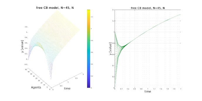
Figure 4: Free dynamics of the system. On the left figure, in the in-plane axes we represent the $N=45$ agents and time rescaled by the factor $1/N^{2}$, while in the vertical axis we draw the full state $y$. In the right picture we represent the same dynamics, drawing the vertical variation of each of the agents positions along the horizontal time variable.

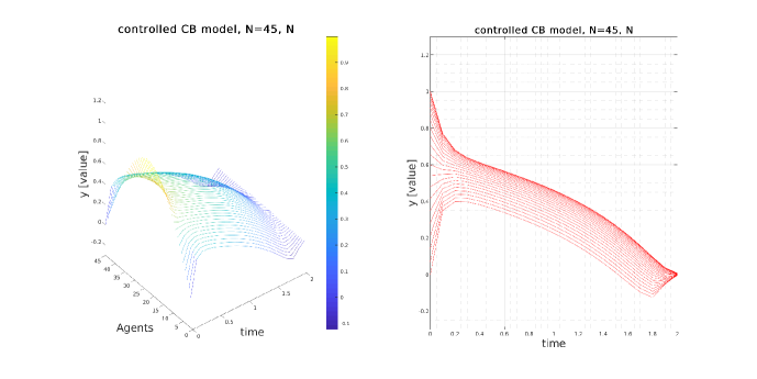
Figure 5: Same as above but for the controlled dynamics.

6 Conclusions and perspectives

We have proved a quantitative result on the approximate controllability for the $N$-agent nonlinear network system (5) in which the state is assured to reach a ball of radius $\exp(-cN)$ around the consensus null state in time $t=N^{2}T$, provided the nonlinearity is scaled by the factor $N^{2}$. We have shown the role that the scaling of the non-linearity and time play in this result.

This result extends earlier ones in Biccari-Zz on the corresponding linear model and it is proved by making use of the semi-discrete Carleman inequalities in RB .

The exponential remainder in the final target we obtain is due to the exponential tail of the Carleman inequalities in RB .

The results in Biccari-Zz , that use the spectral decomposition of solutions of the linear system under consideration, are stronger since they assure that the consensus state is reached exactly. But they are limited to the linear setting.

Within this framework we can quantify the cost of control to consensus showing that it remains uniformly bounded as $N\to\infty$ for an appropriate scaling of the nonlinearity and the time horizon.

Our results apply for non-local nonlinearities, under the same scaling, provided the nonlinearities are uniform on $N$.

The contents of this paper raise some interesting open problems. Among them the following ones are worth underlying:

1. The network we have considered is particularly simple, all agents being aligned and interconnected by dominant linear constant diffusion. The problem of extending these results to more general networks is extremely challenging. This would require, in particular, extending the Carleman inequalities in RB to semi-discrete systems in general networks.

2. Getting rid of the exponential tail at the final time is a challenging problem.

3. We have mainly considered nonlinearities that are globally Lipschtiz. Extending the results in this paper to nonlinearities that grow superlinearly at infinity would require further work.

7 Acknowledgements

This work has been partially funded by the European Research Council (ERC) under the European Union’s Horizon 2020 research and innovation program (grant agreement No. 694126-DyCon), grant MTM2017-92996 of MINECO (Spain), the Marie Curie Training Network “Conflex”, the ELKARTEK project KK-2018/00083 ROAD2DC of the Basque Government, ICON of the French ANR and “Nonlocal PDEs: Analysis, Control and Beyond”, AFOSR Grant FA9550-18-1-0242.

References

• (1) DeustoTech: DyCon Toolbox. https://deustotech.github.io/dycon-platform-documentation/
• (2) Null and approximate controllability for weakly blowing up semilinear heat equations. Annales de l’Institut Henri Poincare (C) Non Linear Analysis 17(5), 583 – 616 (2000). DOI 10.1016/S0294-1449(00)00117-7
• (3) From particle to kinetic and hydrodynamic descriptions of flocking. Kinetic & Related Models 1(1937-5093_2008_3_415), 415 (2008). DOI 10.3934/krm.2008.1.415
• (4) The kuramoto model in complex networks. Physics Reports 610, 1 – 98 (2016). DOI 10.1016/j.physrep.2015.10.008. The Kuramoto model in complex networks
• (5) Biccari, U., Ko, D., Zuazua, E.: Dynamics and control for multi-agent networked systems: a finite difference approach. arXiv Math. to appear in M3AS (2019). URL https://arxiv.org/pdf/1902.03598.pdf
• (6) Boyer, F., Le Rousseau, J.: Carleman estimates for semi-discrete parabolic operators and application to the controllability of semi-linear semi-discrete parabolic equations. Annales de l’I.H.P. Analyse non linéaire 31(5), 1035–1078 (2014). DOI 10.1016/j.anihpc.2013.07.011
• (7) Cañizo, J.A., Carrillo, J.A., Rosado, J.: A well-posedness theory in measures for some kinetic models of collective motion. Mathematical Models and Methods in Applied Sciences 21(03), 515–539 (2011). DOI 10.1142/S0218202511005131
• (8) Coron, J.M.: Control and Nonlinearity. American Mathematical Society, Boston, MA, USA (2007)
• (9) Cucker, F., Smale, S.: Emergent behavior in flocks. IEEE Transactions on Automatic Control 52(5), 852–862 (2007). DOI 10.1109/TAC.2007.895842
• (10) Fattorini, H., Russell, D.: Uniform bounds on biorthogonal functions for real exponentials with an application to the control theory of parabolic equations. Quarterly of Applied Mathematics 32 (1974). DOI 10.1090/qam/510972
• (11) Fattorini, H.O., Russell, D.L.: Exact controllability theorems for linear parabolic equations in one space dimension. Archive for Rational Mechanics and Analysis 43(4), 272–292 (1971). DOI 10.1007/BF00250466
• (12) Fernández-Cara, E., Zuazua, E.: The cost of approximate controllability for heat equations: the linear case. Adv. Differential Equations (4-6), 465–514
• (13) Kearns, D.: A field guide to bacterial swarming motility. Nature reviews. Microbiology 8(9)
• (14) Kuramoto, Y.: Self-entrainment of a population of coupled non-linear oscillators. In: H. Araki (ed.) Mathematical Problems in Theoretical Physics, Lecture Notes in Physics, Berlin Springer Verlag, vol. 39, pp. 420–422 (1975). DOI 10.1007/BFb0013365
• (15) Liu, Y., J.Slotine, Barabási, A.: Controllability of complex networks. Nature 473, 167–173 (2011). DOI 10.1038/nature10011
• (16) Liu, Y.Y., Barabási, A.L.: Control principles of complex systems. Rev. Mod. Phys. 88, 035006 (2016). DOI 10.1103/RevModPhys.88.035006
• (17) Olfati-Saber, R., Fax, J.A., Murray, R.M.: Consensus and cooperation in networked multi-agent systems. Proceedings of the IEEE 95(1), 215–233 (2007). DOI 10.1109/JPROC.2006.887293
• (18) Piccoli, B., Rossi, F., Trélat, E.: Control to flocking of the kinetic cucker–smale model. SIAM Journal on Mathematical Analysis 47(6), 4685–4719 (2015). DOI 10.1137/140996501
• (19) Sontag, E.D.: Mathematical Control Theory: Deterministic Finite Dimensional Systems (2Nd Ed.). Springer-Verlag, Berlin, Heidelberg (1998)
• (20) Sorrentino, F., Di Bernardo, M., Garofalo, F., Chen, G.: Controllability of complex networks via pinning. Physical Review E 75(4), 046103 (2007)