INR-TH-2019-003 Photon splitting constraint on Lorentz Invariance Violation from Crab Nebula spectrum

Abstract

We calculate the decay width of the photon splitting into three photons in a model of quantum electrodynamics with broken Lorentz invariance. We show that this process can lead to a cut-off in the very-high-energy part of a photon spectra of astrophysical sources. We obtain the 95% CL bound on the Lorentz violating mass scale for photons from the analysis of the very-high-energy part of the Crab Nebula spectrum, obtained by HEGRA. This bound improves previous constraints by more than an order of magnitude.

1 Introduction

Lorentz invariance (LI) is one of the most fundamental principles of particle physics. However, in several theoretical models it can be broken. These models are mostly motivated by different approaches to construct the quantum theory of gravity (see review [1] and references therein). According to some approaches [2, 3, 4], deviations from LI, tiny at laboratory energies, increase rapidly with energy and become large at a certain energy scale $M_{LV}$.

The most common approach is to consider Lorentz invariance violation (LV) in the matter sector in the framework of effective field theory (EFT) [5, 6, 7, 8, 9]. In this framework the existence of the preferred frame is assumed. The generic effect of LV for particles is the modification of dispersion relations. At energies much smaller than the LV scale $M_{LV}$ the dispersion relation for a certain particle can be expanded in powers of its momentum. Thus, for photons, we have:

$$E_{\gamma}^{2}=k_{\gamma}^{2}+\sum_{n}\left(\pm\xi_{n}\right)\frac{k_{\gamma}^{n+2}}{M_{LV}^{n}}.$$ (1)

where $\xi_{n}$ are parameters assumed to be of the order of unity, the sign of $\xi_{n}$ is shown explicitly. The first non-zero correction term in Eq. (1) is the leading one. The commonly considered cases are $n=1$ (cubic term) and $n=2$ (quartic term). In the class of models, preserving CPT, the cubic term is absent, so the quartic term is the leading one.

Possible violation of LI for photons may be tested in several ways. First, nontrivial photon dispersion may be tested in timing observations of variable distant sources [10]. Second, cross-sections of reactions involving particles with LV dispersion relation are modified [5, 7, 11, 12]. Physical processes involving photons with modified dispersion relation (1) can be classified by two kinematic types: the sign “$+$” is related to superluminal LV, sign “$-$” — to subluminal case. It is convenient to introduce effective photon mass,

$$m^{2}_{\gamma,eff}\equiv E_{\gamma}^{2}-k_{\gamma}^{2},$$ (2)

that is associated with superluminal and subluminal photons for $m^{2}_{\gamma,eff}>0$ and $m^{2}_{\gamma,eff}<0$ respectively. The processes, constraining the subluminal LV such as pair production on soft photon background[13, 14, 15, 16, 17, 19] and in Coulomb field[20, 12, 21] have been discussed elsewhere. In the present paper we focus on the superluminal case.

Important constraints in the superluminal case come from the photon decay to electron-positron pair $\gamma\to e^{+}e^{-}$. Indeed, energy-momentum conservation implies that this process becomes allowed if the photon effective mass exceeds the double electron mass [5], $m_{\gamma,eff}\geq 2m_{e}$. The equality determines an energy threshold for this reaction, which means that the photons with energy lower than the threshold do not decay. For energies larger than the threshold, the photon decay occurs very rapidly [12].

However, even if the decay $\gamma\to e^{+}e^{-}$ is forbidden, a photon with superluminal dispersion relation is not a stable particle. The corresponding decay channel is photon splitting to several photons, $\gamma\to N\gamma$. In the context of LV, photon splitting was considered in quantum electrodynamics (QED) with additional Chern-Simons term in [22], and for the case of cubic photon dispersion relation in [23] ($n=1$ in (1)).

In the standard Lorentz Invariant QED the process of photon splitting does not occur due to the energy-momentum conservation as all outgoing photon momenta must be parallel. In this configuration the phase volume, as well as the amplitude, is equal to zero.

In the presence of LV the photon dispersion relation is modified (1), and the kinematical configuration for splitting, determined by the energy-momentum conservation, changes. The key feature of dispersion relation (1) for splitting is that the photon effective mass (2) depends on its energy faster than linearly. In this case the energy-momentum conservation implies that the sum of effective masses for outgoing photons is less than the effective mass for the initial photon $\sum_{i}m^{out}_{eff,\,i}<m_{eff}^{in}$. The photon splitting has no threshold: it is kinematically allowed whenever the dispersion relation (1) is superluminal. However, the rate of photon splitting is significantly suppressed compared to the rate of photon decay. The main reason is that the corresponding process has a small phase volume of the outgoing particles.

At first glance it seems that the photon splitting into two photons, $\gamma\to 2\gamma$, is the leading order splitting process. In LI QED the corresponding matrix element is exactly zero due to the cancellation of fermionic and anti-fermionic loops, which is the statement of the Furry theorem. If CPT-parity in the fermion sector of the model is broken, the Furry theorem does not hold anymore. However, even in this case the splitting width acquires additional suppression factor, see a discussion in [1]. Moreover, if the model contains photons with only two transverse polarizations as in the standard case, the splitting channel $\gamma\to 2\gamma$ is forbidden due to helicity conservation.

Thus, the main splitting process is the photon decay into 3 photons, $\gamma\to 3\gamma$. The estimation for the decay width of this process in terms of the photon effective mass (2) was done in Ref. [23]. The authors treated the initial photon as a massive particle with the effective mass defined by (2), while three outgoing photons were considered to be massless. First, the width of the splitting process was estimated in an artificial “rest frame” of the initial photon. Dimensionless phase space integral of the matrix element has not been computed explicitly but considered as a parameter of the order of unity. Second, the authors of Ref. [23] made a boost into the laboratory frame, multiplying the splitting width to the inverse gamma-factor, $m_{\gamma,eff}/E_{\gamma}$. Thus, the estimation for the splitting rate [23] reads,

$$\Gamma_{\gamma\to 3\gamma}\simeq\left(\frac{2\alpha^{2}}{45}\right)^{2}\frac{1}{3!2^{11}\pi^{9}}\frac{m_{\gamma,eff}^{10}}{m_{e}^{8}E_{\gamma}}\,\times\,f,$$ (3)

where $m^{2}_{\gamma}$ is determined by (2) and $f$ is a dimensionless phase volume which has not been computed in [23]. Thus, the estimation of [23] is order of magnitude, so that more accurate calculation of the splitting rate seems to be necessary. In our paper we perform direct calculation of the photon splitting width in the laboratory frame, integrating properly the phase space volume of the outgoing photons. In addition, we obtain momentum distribution for the splitting products which cannot be properly obtained by the estimation of [23].

The article is organized as follows. In Sec.2 we describe the model and Feynman rules. In Sec.3 we calculate the matrix element of the splitting process and integrate it over the phase volume. Sec.4 is devoted to establishing constraints on LV mass scale from Crab nebula spectrum, in Sec. 5 we present discussion.

2 The model.

In order to perform direct calculation one must start from the Lagrangian formalism. The Lagrangian, appropriate to the dispersion relation (1) with $n=2$ and sign $+$ before LV term, is

$$\mathcal{L}=-\frac{1}{4}F_{\mu\nu}F^{\mu\nu}-\frac{1}{2M_{LV}^{2}}F_{ij}\Delta^{2}F^{ij}+i\bar{\psi}\gamma^{\mu}D_{\mu}\psi-m\bar{\psi}\psi,\quad\qquad E_{\gamma}^{2}=k_{\gamma}^{2}+\frac{k_{\gamma}^{4}}{M_{LV}^{2}}.$$ (4)

Here we rewrote the dispersion relation for a photon as well. One may also consider in Lagrangian (4) terms, violating LI for electrons. However, we will omit them for the following reason. Indeed, the bound on LV mass scale for electron $M_{LV,\,e}$ is set at the level of $10^{16}\,\mbox{GeV}$ in [26], while the current limits [27, 28] on $M_{LV}$ for photons are of the order of $10^{11}-10^{12}\,\mbox{GeV}$.

The model (4) corresponds to the most general model called non-minimal SME [29] with a single nonzero coefficient $c^{(6)}_{(I)00}=-\sqrt{\pi}/M_{LV}^{2}$. On the other hand, the model (4) coincides with that of [12], in which fermions are set to be LI. All Feynman rules necessary for perturbative calculation in this model were obtained in [12]. In particular, polarization sums for photons can be written as

$$\sum_{s=1,2}\varepsilon_{\mu}^{*(s)}(k_{\gamma})\varepsilon^{(s)}_{\nu}(k_{\gamma})=-g_{\mu\nu}-\frac{E_{\gamma}^{2}}{M_{LV}^{2}}u_{\mu}u_{\nu},$$ (5)

where $u_{\mu}=(1,0,0,0)$ is unit timelike 4-vector. In the LI limit $M_{LV}\to\infty$ the standard result is restored.

Integrating out electrons produces an effective four-photon vertex that can be read off the Euler-Heisenberg Lagrangian,

$$\mathcal{L}_{E\mbox{-}H}=\frac{2\alpha^{2}}{45m_{e}^{4}}\left[\left(\frac{1}{2}F_{\mu\nu}F^{\mu\nu}\right)^{2}+7\left(\frac{1}{8}\epsilon^{\mu\nu\rho\sigma}F_{\mu\nu}F_{\rho\sigma}\right)^{2}\right].$$ (6)

This form of Euler-Heisenberg Lagrangian is applicable in the limit $m_{\gamma,eff}\ll m_{e}$ – far from the threshold of photon decay.

Let us provide the current photon decay limit for model (1). Photon effective mass is expressed as $m^{2}_{\gamma,eff}=\frac{E_{\gamma}^{4}}{M_{LV}^{2}}$. Hence, detection of a photon with energy $E_{\gamma}$ establishes the constraint $M_{LV}>\frac{E_{\gamma}^{2}}{2m_{e}}\;$. The recent analysis [28] using the highest-energy photons observed from the Crab nebula sets the constraint,

$$M_{LV}>2.8\times 10^{12}\,\mbox{GeV}.$$ (7)

Let us compare the constraint (7) with the estimation for photon splitting constraint from Ref. [23]. Although in Ref. [23] the numerical estimations for the constraint were performed only for the cubic dispersion relation, $n=1$, in the formalism of effective masses (see (3)) they can be easily transferred to the quartic, $n=2$. Thus, using the fact that the photon with energy of $50$ TeV have not been splitted during their propagation from Crab nebula, and the estimation (3) with quartic photon dispersion relation (4), we can estimate the bound on $M_{LV}$ of the order of $10^{13}$ GeV. This expected limit is order of magnitude higher than the bound from the absence of the photon decay (7). Therefore, the splitting process is relevant for setting a more stringent constraint on $M_{LV}$ than the process of decay to $e^{+}e^{-}$ pair. So that, it is instructive to perform accurate direct calculation of the splitting width in the laboratory frame, and set more precise bound on $M_{LV}$. The latter is the focus of the present paper.

3 Decay width

In this section we calculate the width of the photon splitting in the model (1), using Euler-Heisenberg Lagrangian (6) for four-photon interaction. Let us first consider the matrix element of the process $\gamma\rightarrow 3\gamma$.

3.1 Matrix element

Given the Euler-Heisenberg Lagrangian (6), one can extract the matrix element of photon splitting process in a straightforward way. The lowest order amplitude for four-photon process can be written as

$$\mathcal{M}=\frac{\alpha^{2}}{90m_{e}^{4}}\left[(k^{1}_{\mu}\varepsilon_{\nu}^{1}-k^{1}_{\nu}\varepsilon_{\mu}^{1})(k^{2}_{\mu}\varepsilon_{\nu}^{2}-k^{2}_{\nu}\varepsilon_{\mu}^{2})(k^{3}_{\rho}\varepsilon_{\lambda}^{3}-k^{3}_{\lambda}\varepsilon_{\rho}^{3})(k_{\rho}\varepsilon_{\lambda}^{*}-k_{\lambda}\varepsilon_{\rho}^{*})\right.+$$

$$+\frac{7}{16}\left[\epsilon^{\mu\nu\rho\lambda}(k^{1}_{\mu}\varepsilon_{\nu}^{1}-k^{1}_{\nu}\varepsilon_{\mu}^{1})(k^{2}_{\rho}\varepsilon_{\lambda}^{2}-k^{2}_{\lambda}\varepsilon_{\rho}^{2})\right]\left[\epsilon^{\alpha\beta\gamma\delta}(k^{3}_{\alpha}\varepsilon_{\beta}^{3}-k^{3}_{\beta}\varepsilon_{\alpha}^{3})(k_{\gamma}\varepsilon_{\delta}^{*}-k_{\delta}\varepsilon_{\gamma}^{*})\right]+$$ (8)

$$+\left.\mbox{permutations}\;\right],\ \ \$$

here $k^{i}_{\mu},\ \ i=1,2,3$ are outgoing photon four-momenta, $k_{\mu}$ is four-momentum for initial photon, $\varepsilon^{i}_{\mu}$ and $\varepsilon_{\mu}$ are the relevant polarization vectors. Note that photon splitting, $\gamma\rightarrow 3\gamma$, is a cross-channel of a well-known process of two photon scattering, $\gamma\gamma\rightarrow\gamma\gamma$. Therefore, the matrix element of interest has the same structure up to the initial momentum redefinition $k\to-k$ (compare with the matrix element for the photon scattering in [31]). However there are two typical differences between the LI and LV cases that must be taken into account. First, the squared four-momenta of external on-shell photons are not equal zero in LV case. Second, the polarization sums of photon are modified by (5).

The evaluation of matrix element (3.1) by taking into account polarization sums (5) and all permutations is somewhat lengthy, so that we apply the following technique for simplifications. Namely, we factorize polarization vectors in the matrix element to apply the modified polarization sums (5) in a straightforward way. Thus, one has

$$\mathcal{M}=\mathcal{M}_{\mu\nu\rho\lambda}(k_{1},k_{2},k_{3},k)\varepsilon_{\mu}(k_{1})\varepsilon_{\nu}(k_{2})\varepsilon_{\rho}(k_{3})\varepsilon_{\lambda}^{*}(k).$$ (9)

The matrix element tensor $\mathcal{M}_{\mu\nu\rho\lambda}$, which is independent on polarization vectors, can be splitted to a normal and dual parts. Such decomposition can be written as

$$\mathcal{M}_{\lambda_{1}\lambda_{2}\lambda_{3}\lambda}=A_{\lambda_{1}\lambda_{2}\lambda_{3}\lambda}+\frac{7}{16}\tilde{A}_{\lambda_{1}\lambda_{2}\lambda_{3}\lambda}.$$ (10)

Each term in (10) is expressed in the following way:

$$A_{\lambda_{1}\lambda_{2}\lambda_{3}\lambda}=8(T_{\lambda_{1}\lambda_{2}}(k_{1},k_{2})T_{\lambda_{3}\lambda}(k_{3},k)+T_{\lambda_{1}\lambda_{3}}(k_{1},k_{3})T_{\lambda_{2}\lambda}(k_{2},k)+T_{\lambda_{1}\lambda}(k_{1},k)T_{\lambda_{3}\lambda_{2}}(k_{3},k_{2})),$$

$$\tilde{A}_{\lambda_{1}\lambda_{2}\lambda_{3}\lambda}=8(\tilde{T}_{\lambda_{1}\lambda_{2}}(k_{1},k_{2})\tilde{T}_{\lambda_{3}\lambda}(k_{3},k)+\tilde{T}_{\lambda_{1}\lambda_{3}}(k_{1},k_{3})\tilde{T}_{\lambda_{2}\lambda}(k_{2},k)+\tilde{T}_{\lambda_{1}\lambda}(k_{1},k)\tilde{T}_{\lambda_{3}\lambda_{2}}(k_{3},k_{2})).$$ (11)

Here we introduced tensors

$$T_{\mu\nu}(k,p)=2(pk)g_{\mu\nu}-2p_{\mu}k_{\nu},\qquad\ \tilde{T}_{\mu\nu}(k,p)=-4k^{\rho}p^{\lambda}\varepsilon^{\mu\nu\rho\lambda}.$$ (12)

Calculating the matrix element (9) squared, we average over initial photon polarization, and sum over final photon polarizations,

$$\overline{\left|\mathcal{M}\right|^{2}}=\frac{1}{2}\sum_{pols}\mathcal{M}^{*}\mathcal{M}=\mathcal{M}^{*}_{\alpha\beta\gamma\delta}\mathcal{M}_{\mu\nu\rho\lambda}\; \sum_{s_{1}}\varepsilon^{*(s_{1})}_{\alpha}(k_{1})\varepsilon^{(s_{1})}_{\mu}(k_{1})\;\sum_{s_{2}}\varepsilon^{*(s_{2})}_{\beta}(k_{2})\varepsilon^{(s_{2})}_{\nu}(k_{2})\;\cdot$$ (13)

$$\cdot \sum_{s_{3}}\varepsilon^{*(s_{3})}_{\gamma}(k_{3})\varepsilon^{(s_{3})}_{\rho}(k_{3})\;\frac{1}{2}\sum_{s}\varepsilon^{(s)}_{\delta}(k)\varepsilon^{*(s)}_{\lambda}(k).$$

Note that the polarization sums $\sum_{s}\varepsilon^{*(s)}_{\mu}(k)\varepsilon^{(s)}_{\nu}(k)$ are given by Eq. (5), the matrix element tensor $\mathcal{M}_{\mu\nu\rho\lambda}$ is determined by eqs. (10)-(12). The calculation (13) was done via FeynCalc package [32, 33] for Wolfram Mathematica. The result for the squared matrix element cannot be given in a short formula and is shown elsewhere [34]. The squared matrix element (13), constrained to LI theory and applied to the cross-channel of splitting, photon scattering $\gamma\gamma\to\gamma\gamma$, agrees with the standard result [31].

3.2 Phase volume integration

In this subsection we discuss the integration of the squared matrix element (13) over 3-particle phase volume in order to calculate the photon splitting decay width. The general textbook formula for the decay width reads

$$\Gamma_{\gamma\to 3\gamma}=\frac{1}{2E}\int\frac{1}{3!}\prod_{i=1,2,3}\frac{d\vec{k}_{i}}{(2\pi)^{3}(2E_{i})}\overline{|\mathcal{M}|^{2}}(2\pi)^{4}\,\delta^{(4)}\left(k-k_{1}-k_{2}-k_{3}\right),$$ (14)

where $E_{i}$ are the energies of outgoing photons $(i=1,2,3)$, and $E$ is the energy of initial photon, which is considered to be small compared to $M_{LV}$, $E\ll M_{LV}$. The factor $1/3!$ in (14) accounts the permutation number of the final photons.

Since our theory does not possess LI, we are not allowed to make a boost to a center-of-mass frame for simplicity. Hence, we have to carry out the calculations in the laboratory frame. We perform integration over final momenta in (14) in cylindric coordinates, dividing the spacial momenta of final photons to longitudinal $k_{i}^{\parallel}$ and transverse $\vec{k}_{i}^{\perp}$ components with respect to the initial photon momentum $k$. Transverse components $\vec{k}_{i}^{\perp}$, in turn, are 2-vectors in a plane, perpendicular to $\vec{k}$. Each of them can be parametrized by the absolute value $|\vec{k}_{i}^{\perp}|$ and polar angle $\varphi_{i}$. One of the polar angles, say $\varphi_{1}$, is a free parameter corresponding to the rotational symmetry around initial photon momentum axis. The momentum conservation law implies that $\vec{k}_{1}^{\perp}+\vec{k}_{2}^{\perp}+\vec{k}_{3}^{\perp}=0$. In terms of absolute values and polar angles, we have:

$$|\vec{k}_{3}^{\perp}|^{2}=|\vec{k}_{1}^{\perp}|^{2}+|\vec{k}_{2}^{\perp}|^{2}+2|\vec{k}_{1}^{\perp}||\vec{k}_{2}^{\perp}|\cos\varphi_{12},$$ (15)

$\varphi_{12}$ denotes the angle between $\vec{k}_{1}^{\perp}$ and $\vec{k}_{2}^{\perp}$. The conservation law for longitudinal momenta implies that $k_{1}^{\parallel}+k_{2}^{\parallel}+k_{3}^{\parallel}=k$.

Note that the phase volume integral (14) vanishes in LI theory since for LI photon dispersion relation $E_{i}^{2}=|\vec{k}^{2}_{i}|$ the delta-functions for energies and longitudinal momenta in (14) coincide, fixing all transverse components $\vec{k}_{i}^{\perp}$ to be exactly zero. In the presence of LV for photons nonzero transverse momenta are allowed. We integrate out 3-momentum $\vec{k}_{3}$ in (14) eliminating spacial part of the delta-function, so the phase volume (14) reads as

$$\Gamma_{\gamma\to 3\gamma}=\frac{1}{2^{9}\,3!\,\pi^{5}}\frac{1}{E}\int\frac{dk^{\parallel}_{1}\,dk^{\parallel}_{2}\,d^{2}k_{1}^{\perp}d^{2}k_{2}^{\perp}}{E_{1}E_{2}E_{3}}\delta(E-E_{1}-E_{2}-E_{3})\overline{|\mathcal{M}|^{2}}.$$ (16)

In order to perform integration in (16) we should first resolve final energies $E_{i}$ through longitudinal and transverse momenta. Thus,

$$E_{i}^{2}=(k^{\parallel}_{i})^{2}+(k_{i}^{\perp})^{2}+\frac{\left((k^{\parallel}_{i})^{2}+(k_{i}^{\perp})^{2}\right)^{2}}{M_{LV}^{2}},\qquad i=1,2,3,$$ (17)

while $E^{2}=k^{2}+\frac{k^{4}}{M_{LV}^{2}}$, $k=\sum_{i}k_{i}^{\parallel}$. Note that generally the squared transverse momenta are of the order of squared effective mass for initial photon but should not exceed it, $(k_{i}^{\perp})^{2}\lesssim\frac{k^{4}}{M_{LV}^{2}}$. Thus, for further calculations we apply the following approximation:

$$k_{i}^{\perp}/k\lesssim k/M_{LV}\ll 1.$$ (18)

We perform our calculations in the leading order in this small parameter. Note that this parameter is associated with typical angle between the momenta of outgoing photons and the initial photon momentum. It is convenient to express the longitudinal $k_{i}^{\parallel}$ and transverse $|\vec{k}_{i}^{\perp}|$ momenta via dimensionless variables $\alpha_{i}$ and $\beta_{i}$

$$k_{i}^{\parallel}=\alpha_{i}k,\qquad|\vec{k}_{i}^{\perp}|=\frac{k^{2}}{M_{LV}}\cdot\beta_{i},\qquad i=1,2,3.$$ (19)

In this notations, energies for outgoing photons, including the first order correction, take the form

$$E_{i}=k\alpha_{i}+\frac{k^{3}}{2M_{LV}^{2}}\left(\alpha^{3}_{i}+\frac{\beta^{2}_{i}}{\alpha_{i}}\right),\ \ i=1,2,$$ (20)

$$E_{3}=k\,(1-\alpha_{1}-\alpha_{2})+\frac{k^{3}}{2M_{LV}^{2}}\left((1-\alpha_{1}-\alpha_{2})^{3}+\frac{\beta_{1}^{2}+\beta_{2}^{2}+2\beta_{1}\beta_{2}\cos\varphi_{12}}{1-\alpha_{1}-\alpha_{2}}\right).$$ (21)

The expressions (19)-(21) should be substituted to the delta-function in (16). We are interested in the leading order term, so we neglect the LV corrections to energies in the denominator of (16). Then the phase volume (16) reads

$$\Gamma_{\gamma\to 3\gamma}\;=\;\frac{1}{2^{9}\,3!\,\pi^{5}}\frac{2\pi}{k}\left(\frac{k^{2}}{M_{LV}}\right)^{4}\int\frac{d\alpha_{1}\,d\alpha_{2}\,d\varphi_{12}d(\beta_{1}^{2})d(\beta_{2}^{2})}{\alpha_{1}\alpha_{2}(1-\alpha_{1}-\alpha_{2})}\ \overline{|\mathcal{M}|^{2}}\ \times$$ (22)

$$\times\;\delta \left[\frac{k^{3}}{2M_{LV}^{2}}\left(3(\alpha_{1}+\alpha_{2})(1-\alpha_{1}-\alpha_{2}+\alpha_{1}\alpha_{2})+\frac{\left(\frac{1-\alpha_{2}}{\alpha_{1}}\beta_{1}^{2}+\frac{1-\alpha_{1}}{\alpha_{2}}\beta_{2}^{2}+2\beta_{1}\beta_{2}\cos\varphi_{12}\right)}{1-\alpha_{1}-\alpha_{2}}\right)\right].$$

Here additional $2\pi$ factor is the result of integration over $\varphi_{1}$. The delta-function in (22) can be removed by taking the integral over $\varphi_{12}$. In what follows we express $\cos\varphi_{12}$ as the function of dimensionless variables

$$\cos\varphi_{12}=\frac{3(\alpha_{1}+\alpha_{2})(1-\alpha_{1}-\alpha_{2})(1-\alpha_{1}-\alpha_{2}+\alpha_{1}\alpha_{2})-\frac{1-\alpha_{2}}{\alpha_{1}}\beta_{1}^{2}-\frac{1-\alpha_{1}}{\alpha_{2}}\beta_{2}^{2}}{2\beta_{1}\beta_{2}}.$$ (23)

Note that the decay width (22) acquires additional factor $\frac{k^{3}}{2M_{LV}^{2}}\frac{2\beta_{1}\beta_{2}}{1-\alpha_{1}\alpha_{2}}\sin\varphi_{12}$ in the denominator. Finally, the decay width reads as

$$\Gamma_{\gamma\to 3\gamma}=\frac{1}{2^{8}\,3!\,\pi^{4}}\frac{k^{4}}{M_{LV}^{2}}\int\frac{d\alpha_{1}\,d\alpha_{2}\,d\beta_{1}d\beta_{2}}{\alpha_{1}\alpha_{2}}\frac{\overline{|\mathcal{M}|^{2}}}{\left.\sin\varphi_{12}\right|_{\varphi_{12}=\varphi_{12}(\alpha_{1},\alpha_{2},\beta_{1},\beta_{2})}}.$$ (24)

Let us specify the integration area for the variables in the phase volume. First, in our approach all longitudinal parts of outgoing photon momenta should be positive, hence, the area of integration over $\alpha_{1},\alpha_{2}$ is a triangle: $\alpha_{1}>0,\,\alpha_{2}>0,\,\alpha_{1}+\alpha_{2}<1$. Second, the integration area spanned by $(\beta_{1},\;\beta_{2})$ is determined by the condition (see (23)):

$$-1<\left.\cos\varphi_{2}\right|_{\varphi_{2}=\varphi_{2}(\alpha_{1},\alpha_{2},\beta_{1},\beta_{2})}<1.$$ (25)

We perform the integration in (24) numerically. The matrix element (13) is evaluated at our kinematical configuration (the explicit result is lengthy and presented in [34]). Fixing longitudinal momenta $(\alpha_{1},\alpha_{2})$, we first perform the integration over transverse parts $(\beta_{1},\;\beta_{2})$. The splitting width density distribution in terms of longitudinal momenta $\alpha_{1},\,\alpha_{2}$ is shown in left panel of Fig. 1. The relevant density distribution has a peak at $\alpha_{1}=\alpha_{2}=1/3$, that is the most probable collinear momenta orientation of the outgoing photons, such that $\alpha_{3}=1/3$. On the other hand, for the fixed $\alpha_{1}\sim 0$ it has local peak at $\alpha_{2}=1/2$. This typical momentum orientation describes the collinearity of two out of three outgoing photons $\alpha_{2}=\alpha_{3}=1/2$ with negligibly small momentum of a third photon $\alpha_{1}=0$. Remarkably, that the latter momentum configuration is not in fact suppressed in comparison with the symmetric configuration $\alpha_{1}=\alpha_{2}=\alpha_{3}=1/3$. Indeed, it corresponds to the phase volume of $\gamma\to\gamma\gamma$ which is not zero. In addition, we note that the probability of processes with one of final photons carrying almost all of the initial energy, say $\alpha_{1}\sim\alpha_{2}\sim 0$, $\alpha_{3}\sim 1$, appears to be strongly suppressed.

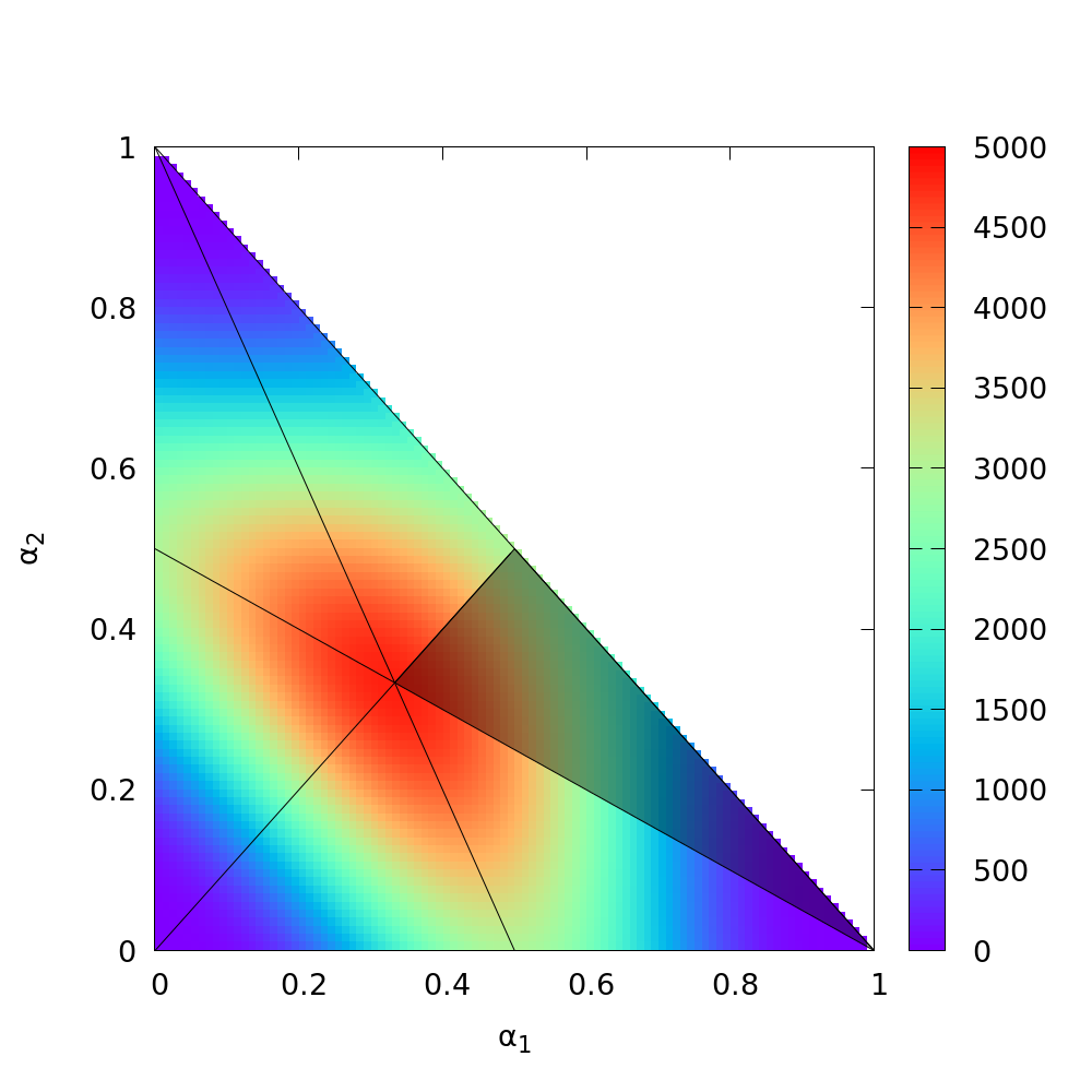
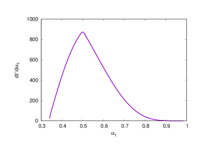
Figure 1: Left panel: The decay width density $d^{2}\Gamma/d\alpha_{1}d\alpha_{2}$ as the function of longitudinal momenta of two outgoing photons $(\alpha_{1},\alpha_{2})$. The maximum is achieved at $\alpha_{1}=\alpha_{2}=1/3$. Shaded region corresponds to the hierarchy $k_{1}>k_{2}>k_{3}$, the width density in other regions is determined through the shaded region via the permutation symmetry. Right panel: The decay width density $d\Gamma/d\alpha_{1}$ as the function of the maximal longitudinal momentum $\alpha_{1}\equiv\alpha_{max}$. The peak is at $\alpha_{1}=0.5$.

One should also note that the symmetry of permutations for final photons $\alpha_{i}\leftrightarrow\alpha_{j},\ i,j=1,2,3,\ i\neq j,\ \alpha_{3}=1-\alpha_{1}-\alpha_{2}$, technically broken in our calculations, has been restored now. In the left panel of Fig. 1 we show the density distribution $d\Gamma/(d\alpha_{1}d\alpha_{2})$ with an ambiguity of $(\alpha_{1},\alpha_{2})$ kinematical configuration. Indeed, the medians of the triangle divide the allowed $(\alpha_{2},\alpha_{1})$-plane into six equivalent density regions.

Integration over remaining variables $\alpha_{1},\alpha_{2}$ gives us the total splitting width,

$$\Gamma_{\gamma\to 3\gamma}\ \simeq\ \,1.2\cdot 10^{3}\left(\frac{2\alpha^{2}}{45}\right)^{2}\frac{1}{2^{8}\,3!\,\pi^{4}}\frac{E_{\gamma}^{19}}{m_{e}^{8}M^{10}_{LV}}\ \ \simeq\ 5\cdot 10^{-14}\;\frac{E_{\gamma}^{19}}{m_{e}^{8}M^{10}_{LV}}.$$ (26)

In fact, the parametric dependence of the splitting width (26) coincides with the estimation of [23], see (3). Thus, we determine the value of $f$ from (3), which is equal to $f\simeq 3\cdot 10^{6}$. The numerical factor in (26) is several orders of magnitude larger than that estimated in (3). It can be attributed to the large symmetry factor from the matrix element.

We must verify that the splitting process could be registered in observations i.e. that, the most energetic decay products would be distinguished from the initial photon which has not undergone splitting. For this reason we calculate the probability density of splitting as the function of maximal photon energy. Thus, we integrate the decay width density (see left panel of Fig. 1) over $\alpha_{2}$. In order to get rid of permutation ambiguity, we fix the hierarchy $\alpha_{1}>\alpha_{2}>\alpha_{3}=1-\alpha_{1}-\alpha_{2}$, denoting first outgoing photon $k_{1}$ as the most energetic, $\alpha_{1}\equiv\alpha_{max}$. This region corresponds to the dark shaded triangle in the left panel of Fig. 1. The result of numerical integrations are presented in the right panel of Fig. 1. Note that the probability distribution peaks when the final photon of maximal energy carries away one half of the initial photon energy, $\alpha_{1}=0.5$. The maximum shifted from $1/3$ to $0.5$. The explanation is the following. There are large number of configurations connected with $\alpha_{1}=0.5$ but only one configuration for $\alpha_{max}=0.33$. The configuration with tiny energy losses (two soft photons) is still strongly suppressed.

4 The constraint from Crab nebula spectrum

Let us discuss the possibility of splitting for ultra-high-energy photons from astrophysical sources. Inverting the width (26), we obtain the photon mean free path associated with the splitting process,

$$\langle L\rangle_{\gamma\to 3\gamma}\simeq 16\times\left(\frac{M_{LV}}{10^{14}\,\mbox{GeV}}\right)^{10}\,\left(\frac{E_{\gamma}}{40\,\mbox{TeV}}\right)^{-19}\ \mbox{Mpc}.$$ (27)

For the typical photon energy $\simeq 40$ TeV and for $M_{LV}\simeq 10^{14}$ GeV the photon mean free path is of extragalactic scales. For a given distance to the source $L_{source}$ there is a cut-off photon energy $E_{cut-off}$, determined by $L\left(\gamma\to 3\gamma\right)\simeq L_{source}$: photons with larger energy decay via splitting. The estimation for the constraint on $M_{LV}$ straightforwardly follows from (27),

$$M_{LV}>\left(\frac{E_{\gamma}}{40\,\mbox{TeV}}\right)^{1.9}\,\left(\frac{L_{source}}{16\,\mbox{Mpc}}\right)^{0.1}\ \times\;10^{14}\;\,\mbox{GeV}.$$ (28)

This bound is applicable if $m_{\gamma,\,eff}\ll m_{e}$, or equivalently

$$M_{LV}\,\gg\,\frac{E_{\gamma}^{2}}{m_{e}}\;\simeq\;\left(\frac{E_{\gamma}}{40\,\mbox{TeV}}\right)^{2}\ \times\ 3\cdot 10^{12}\;\,\mbox{GeV}\,.$$ (29)

One can see that the bound (28) is stronger than the condition (29). Furthermore, the bound (28) is sensitive to the initial photon energy $\sim E_{\gamma}^{1.9}$. On the other hand, this limit weakly depends on the source distance $\sim L_{source}^{0.1}$. Thus, more energetic but less distant galactic source can set better constraint on $M_{LV}$ than less energetic but more distant extragalactic source. Let us illustrate it numerically for the galactic Crab nebula ($L_{source}=2$ kpc, maximal photon energy $E_{\gamma,max}=75$ TeV [30]); and the most energetic extragalactic blazar Mrk 501 ($L_{source}=140$ Mpc, $E_{\gamma,max}=20$ TeV [35]). Formula (28) reads,

$$\mbox{Crab}:\qquad M_{LV}>1.3\cdot 10^{14}\,\mbox{GeV},$$ (30)

$$\mbox{Mrk}501:\qquad M_{LV}>3\cdot 10^{13}\,\mbox{GeV}.$$ (31)

The estimated bound from the galactic Crab nebula is 4 times better than from the extragalactic source. Let us perform simple statistical analysis in order to make the bound (31) more precise. For this reason we analyze Crab data obtained by HEGRA [30]. We closely follow the analysis of Ref. [21].

A single splitting process obeys exponential probability distribution. Thus, the photon traveling from Crab nebula to Earth does not undergo the splitting with the probability

$$P(E)=\mbox{e}^{-L_{CRAB}/\langle L\rangle_{\gamma\to 3\gamma}},$$ (32)

here $L_{CRAB}$ is the distance to Crab Nebula and the photon mean free path $\langle L\rangle_{\gamma\to 3\gamma}$ is determined by (27). We expect that the observed Crab Nebula spectrum $d\Phi/dE$ would be corrected by factor of (32),

$$\left(\frac{d\Phi}{dE}\right)_{LV}=P(E)\cdot\left(\frac{d\Phi}{dE}\right)_{source}.$$ (33)

The effect of splitting suppression on the HEGRA Crab spectrum [30] is illustrated in Fig.2, left panel. We take observational data for photon spectra and use the power-law fit fixed by data points at energies below 20 TeV, $\frac{d\Phi}{dE}\sim E^{-2.62}$. We make predictions to the detectable Crab nebula flux under hypothesis of a certain $M_{LV}$. The break in the highest-energy tail at energy $E_{cut-off}$ of spectrum is clearly seen at Fig.2. One can expect also an excess in the spectrum, associated with final products of splitting, located near energy $E_{cut-off}/2$. However, for spectra which decrease stronger than $\frac{d\Phi}{dE}\propto E^{-2}$ the flux of splitting products at energy $E_{cut-off}/2$ would be less than the flux from the source of that energy. Thus, for Crab nebula, whose spectrum decreases even faster the excess would be negligible small.

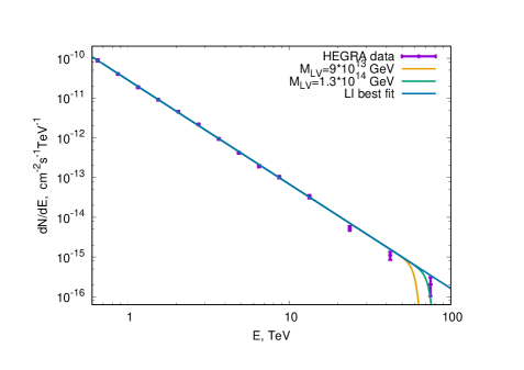
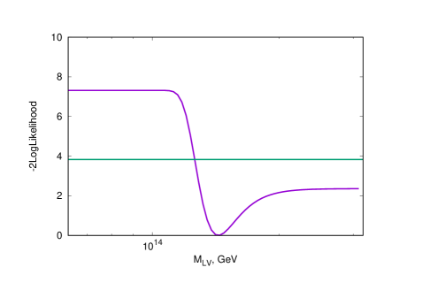
Figure 2: Left panel: photon spectrum of the Crab nebula obtained by collaboration HEGRA[30]. The dashed line corresponds to the best power-law fit of the spectrum while the dotted lines show the prediction for the flux under the hypothesis of Lorentz violation with a given $M_{LV}$. Right panel: dependence of the likelihood on the LV mass scale $M_{LV}$.

We test the family of LV hypotheses parametrized by $M_{LV}$ with HEGRA data[30] for the last bin of Crab nebula spectrum, centered at $75$ TeV. For this reason we apply likelihood ratio method [36, 37]. More precisely, we test the expectation value for signal events under the hypothesis of LV in the last energy bin with the observed value for signal events, marginalizing over background with unknown expectation value. Details of the analysis are described in [21]. The obtained likelihood profile is shown in Fig. 2, right panel. From it one reads the constraint

$$M_{LV}>1.3\times 10^{14}\,\mbox{GeV}\qquad 95\%$$ at CL, (34)

or, in the parametrization of [29],

$$c^{(6)}_{(I)00}>-1.1\,\times\,10^{-28}\;\ \mbox{GeV}^{-2}\qquad\qquad\qquad\ \text{at $95\%$ CL}.$$ (35)

This constraint is almost two order of magnitude better than obtained from the absence of photon decay (7).

5 Discussion

We have calculated the width of the photon splitting process $\gamma\to 3\gamma$, in LV QED with superluminal photons. We have shown that the splitting process is the leading LV phenomenon in superluminal case that would lead to a to cut-off in spectra for galactic sources. Using experimental data for Crab spectrum, obtained by HEGRA, we obtained $95\%$ CL lower bounds on the LV mass scale for superluminal dispersion relation for photons. This bound improves previous constraints by more than an order of magnitude.

The ability to constrain $M_{LV}$ from splitting process grows with photon energy as $E_{\gamma}^{1.9}$. Thus, possible detection of photons with energy exceeding $75$ TeV from a source will set stronger constraints. Crab nebula photon spectrum, according to different theoretical models, continues up to $100$-$400$ TeV [38]. At these energies, it would be detected by HAWC[39], CTA[40, 41], Carpet-2[42], TAIGA[43], LHAASO[44]. Detection of photons from Crab (or other galactic sources) in these energy range may increase the bound (34) up to the level $M_{LV}>5\times 10^{14}\,\mbox{GeV}$.

Increasing photon energy significantly more, we can speculate about possible splitting of ultra-high-energy photons in energy range $10^{18}-10^{19}\,\mbox{eV}$ which can be expected as one of the final products of the Greizen-Zatsepin-Kuzmin (GZK) process [45, 46] – pion production by proton scattering on cosmic microwave background. These GZK, or cosmogenic photons, also can scatter on CMB or radio background. However, a part of the GZK photon flux can reach the Earth. Pierre Auger Observatory or Telescope Array experiments are able to detect predicted flux of GZK photons in near future [47, 48], but there are no detected signal yet [49, 50].

It is known that GZK photons would immediately decay to $e^{+}e^{-}$ pair in presence of LV of superluminal type [51]. Furthermore, possible observation of a photon with energy $\sim 10^{19}$ eV will set a very strong transplankian constraint $M_{LV}>10^{23}$ GeV [51]. However, the splitting decay channel is still dominating at this energies. It follows from (28) that future detection of GZK photons $\sim 10^{19}$ eV from GZK horizon $L_{source}\sim 50$ Mpc, will establish the constraint $M_{LV}>10^{24}$ GeV. This estimated constraint is an order of magnitude better than the bound from the absence of photon decay to $e^{+}e^{-}$ pair. However, in order to make a precise constraint both processes of photon production during GZK process and propagation with scattering on cosmic microwave and radio backgrounds should be taken into account in details.

We also should point out that for qualitative predictions for splitting at these energies we must take into account LV terms for electrons which will produce extra LV terms in the Euler-Heisenberg Lagrangian. Detailed computation is out of scope of this article. We leave this interesting task for future.

Acknowledgements

We are very grateful to Sergey Sibiryakov, Grigory Rubtsov, Mikhail Kuznetsov and Mikhail Vysotsky for helpful discussions.

References

- [1] S. Liberati, Class. Quant. Grav. 30, 133001 (2013).
- [2] J. R. Ellis, N. E. Mavromatos, D. V. Nanopoulos and A. S. Sakharov, Int. J. Mod. Phys. A 19 (2004) 4413 [gr-qc/0312044]; N. E. Mavromatos, Int. J. Mod. Phys. A 25 (2010) 5409 [arXiv:1010.5354 [hep-th]].
- [3] P. Horava, Phys. Rev. D 79 (2009) 084008 [arXiv:0901.3775 [hep-th]].
- [4] F. Girelli, F. Hinterleitner and S. Major, SIGMA 8, 098 (2012) [arXiv:1210.1485 [gr-qc]].
- [5] S. R. Coleman and S. L. Glashow, Phys. Lett. B 405, 249 (1997).
- [6] D. Colladay and V. A. Kostelecky, “Lorentz violating extension of the standard model,” Phys. Rev. D 58 (1998) 116002. [hep-ph/9809521].
- [7] T. Jacobson, S. Liberati and D. Mattingly, Phys. Rev. D 67, 124011 (2003) [hep-ph/0209264]; Annals Phys. 321, 150 (2006) [astro-ph/0505267].
- [8] R. C. Myers and M. Pospelov, Phys. Rev. Lett. 90 (2003) 211601 [hep-ph/0301124].
- [9] V. A. Kostelecky and M. Mewes, Phys. Rev. Lett. 99 (2007) 011601 [astro-ph/0702379].
- [10] S. D. Biller et al., Phys. Rev. Lett. 83, 2108 (1999) [gr-qc/9810044].
- [11] D. Colladay and V. A. Kostelecky, Phys. Lett. B 511 (2001) 209 doi:10.1016/S0370-2693(01)00649-9 [hep-ph/0104300].
- [12] G. Rubtsov, P. Satunin and S. Sibiryakov, Phys. Rev. D 86 (2012) 085012 doi:10.1103/PhysRevD.86.085012 [arXiv:1204.5782 [hep-ph]].
- [13] T. Kifune, Astrophys. J. 518 (1999) L21 [astro-ph/9904164].
- [14] F. W. Stecker and S. L. Glashow, Astropart. Phys. 16 (2001) 97 [astro-ph/0102226].
- [15] F. W. Stecker, Astropart. Phys. 20 (2003) 85 [astro-ph/0308214].
- [16] U. Jacob and T. Piran, Phys. Rev. D 78 (2008) 124010 [arXiv:0810.1318 [astro-ph]].
- [17] F. Tavecchio and G. Bonnoli, Astron. Astrophys. 585 (2016) A25 [arXiv:1510.00980 [astro-ph.HE]].
- [18] J. Biteau and D. A. Williams, Astrophys. J. 812 (2015) no.1, 60 [arXiv:1502.04166 [astro-ph.CO]].
- [19] H. Abdalla et al. [H.E.S.S. Collaboration], Astrophys. J. 870 (2019) no.2, 93 doi:10.3847/1538-4357/aaf1c4 [arXiv:1901.05209 [astro-ph.HE]].
- [20] H. Vankov and T. Stanev, Phys. Lett. B 538 (2002) 251 [astro-ph/0202388].
- [21] G. Rubtsov, P. Satunin and S. Sibiryakov, JCAP 1705 (2017) 049 doi:10.1088/1475-7516/2017/05/049 [arXiv:1611.10125 [astro-ph.HE]].
- [22] C. Adam and F. R. Klinkhamer, Nucl. Phys. B 657 (2003) 214 doi:10.1016/S0550-3213(03)00143-3 [hep-th/0212028].
- [23] G. Gelmini, S. Nussinov and C. E. Yaguna, JCAP 0506 (2005) 012 doi:10.1088/1475-7516/2005/06/012 [hep-ph/0503130].
- [24] S. L. Adler, Annals Phys. 67 (1971) 599. doi:10.1016/0003-4916(71)90154-0
- [25] Z. Bialynicka-Birula and I. Bialynicki-Birula, Phys. Rev. D 2 (1970) 2341. doi:10.1103/PhysRevD.2.2341
- [26] S. Liberati, L. Maccione and T. P. Sotiriou, Phys. Rev. Lett. 109 (2012) 151602 doi:10.1103/PhysRevLett.109.151602 [arXiv:1207.0670 [gr-qc]].
- [27] V. Vasileiou et al., Phys. Rev. D 87 (2013) no.12, 122001 doi:10.1103/PhysRevD.87.122001 [arXiv:1305.3463 [astro-ph.HE]].
- [28] H. Martínez-Huerta and A. Pérez-Lorenzana, “Restrictive scenarios from Lorentz Invariance Violation to cosmic rays propagation,” arXiv:1610.00047 [astro-ph.HE].
- [29] V. A. Kostelecky and M. Mewes, Phys. Rev. D 80 (2009) 015020 [arXiv:0905.0031 [hep-ph]].
- [30] F. Aharonian et al. [HEGRA Collaboration], Astrophys. J. 614 (2004) 897 doi:10.1086/423931 [astro-ph/0407118].
- [31] M. Schwartz. QFT and the Standard Model. Cambridge University Press, 2013.
- [32] R. Mertig, M. Bohm and A. Denner, Comput. Phys. Commun. 64 (1991) 345. doi:10.1016/0010-4655(91)90130-D
- [33] V. Shtabovenko, R. Mertig and F. Orellana, Comput. Phys. Commun. 207 (2016) 432 doi:10.1016/j.cpc.2016.06.008 [arXiv:1601.01167 [hep-ph]].
- [34] https://github.com/asapovk/photon_splitting_calculation
-
[35]
F. Aharonian [HEGRA Collaboration],
Astron. Astrophys. 349 (1999) 11
[astro-ph/9903386].
F. Aharonian [HEGRA Collaboration], Astron. Astrophys. 366 (2001) 62 [astro-ph/0011483]. - [36] T.-P. Li and Y.-Q. Ma, Astrophys. J. 272 (1983) 317.
- [37] W. A. Rolke, A. M. Lopez and J. Conrad, Nucl. Instrum. Meth. A 551 (2005) 493 [physics/0403059].
- [38] M. Meyer, D. Horns and H.-S. Zechlin, Astron. Astrophys. 523, A2 (2010) [arXiv:1008.4524 [astro-ph.HE]].
-
[39]
A. U. Abeysekara et al. [HAWC Collaboration],
“HAWC Contributions to the 34th International Cosmic Ray Conference
(ICRC2015),”
arXiv:1508.03327 [astro-ph.HE].
http:/www.hawc-observatory.org - [40] B. S. Acharya et al., Astropart. Phys. 43, 3 (2013).
- [41] K. Bernlöhr et al., Astropart. Phys. 43, 171 (2013) [arXiv:1210.3503 [astro-ph.IM]].
-
[42]
D. D. Dzhappuev, V. B. Petkov, A. U. Kudzhaev, N. F. Klimenko,
A. S. Lidvansky and S. V. Troitsky,
arXiv:1511.09397 [astro-ph.HE].
D. D. Dzhappuev et al., arXiv:1812.02663 [astro-ph.HE]. - [43] N. Budnev et al., “The TAIGA experiment: from cosmic ray to gamma-ray astronomy in the Tunka valley,” J. Phys. Conf. Ser. 718 (2016) no.5, 052006.
- [44] G. Di Sciascio [LHAASO Collaboration], “The LHAASO experiment: from Gamma-Ray Astronomy to Cosmic Rays,” arXiv:1602.07600 [astro-ph.HE].
- [45] K. Greisen, Phys. Rev. Lett. 16 (1966) 748.
- [46] G. T. Zatsepin and V. A. Kuzmin, JETP Lett. 4 (1966) 78.
- [47] G. Gelmini, O. E. Kalashev and D. V. Semikoz, J. Exp. Theor. Phys. 106 (2008) 1061.
- [48] R. Alves Batista, R. M. de Almeida, B. Lago and K. Kotera, JCAP 1901 (2019) no.01, 002 doi:10.1088/1475-7516/2019/01/002 [arXiv:1806.10879 [astro-ph.HE]].
- [49] R. U. Abbasi et al. [Telescope Array Collaboration], arXiv:1811.03920 [astro-ph.HE].
- [50] P. Homola [Pierre Auger Collaboration], CERN Conf. Proc. 1 (2018) 283 doi:10.23727/CERN-Proceedings-2018-001.283 [arXiv:1804.05613 [astro-ph.IM]].
- [51] M. Galaverni and G. Sigl, Phys. Rev. D 78 (2008) 063003 doi:10.1103/PhysRevD.78.063003 [arXiv:0807.1210 [astro-ph]].
- [52] A. Kostelecky and Z. Li, arXiv:1812.11672 [hep-ph].