Revisiting the Kepler non-Blazhko RR Lyrae sample: Cycle-to-cyle variations and additional modes

Abstract

We analyzed the long and short cadence light curves of the Kepler non-Blazhko RRab stars. We prepared the Fourier spectra, the Fourier amplitude and phase variation functions, time-frequency representation, the O$-$C diagrams and their Fourier contents. Our main findings are: (i) All stars which are brighter a certain magnitude limit show significant cycle-to-cycle light curve variations. (ii) We found permanently excited additional modes for at least one third of the sample and some other stars show temporarily excited additional modes. (iii) The presence of the Blazhko effect was carefully checked and identified one new Blazhko candidate but for at least 16 stars the effect can be excluded. This fact has important consequences. Either the cycle-to-cycle variation phenomenon is independent from the Blazhko effect and the Blazhko incidence ratio is still much lower (51%-55%) than the extremely large (>90%) ratio published recently. The connection between the extra modes and the cycle-to-cycle variations is marginal.

1 Introduction

When the first pulsating variable stars were discovered at the end of the 19th century, seeing their accurately repetitive light curves, it was even suggested that they could be the basis of the time measurement as standard oscillators. The discovery of incredible accuracy of the atomic vibration frequencies made all such suggestions of the past. With the development of stellar pulsation and evolution theories it became evident that the periods of pulsating variables are changing during their evolution. This type of variation was intensively searched in the first half of the past century. The main tool of this work was the O$-$C diagram (see Sterken 2005 and references therein). The decades or century-long diagrams of RR Lyrae stars, however, yielded rather controversial results. Only the smaller part of the investigated stars showed evolution origin period change, the larger part showed irregular large amplitude period variations (e.g. Szeidl 1965, 1973; Barlai 1989).

A possible explanation of this finding was the sum up of the small random changes of the pulsation cycles. In other words: we see random walk in O$-$C diagrams (Balázs-Detre & Detre, 1965; Koen, 2006). Later, several authors suggested possible irregular changes in the period of the classic radially pulsating variables (Cepheids and RR Lyrae type) on various theoretical bases (Sweigart & Renzini, 1979; Deasy & Wayman, 1985; Cox, 1998). These ideas, however, have never been included into any standard pulsation codes.

The more recent and more extended period change studies of RR Lyrae stars in the Galactic field and globular clusters (Le Borgne et al., 2007; Jurcsik et al., 2001, 2012; Szeidl et al., 2011) came to the conclusion that most of the non-Blazhko stars show smooth evolution origin period changes while Blazhko stars have large amplitude short time-scale irregular period fluctuations. The possibility of cycle-to-cycle variation of the non-Blazhko stars has been removed from the agenda.

The first direct detection of a random period jitter of V1154 Cyg, the only classical Cepheid of the original Kepler field (Derekas et al., 2012, 2017), however, changed the situation. A similar phenomenon was suspected for CM Ori a mono-periodic (non-Blazhko) RR Lyrae star observed by the CoRoT space telescope (Benkő et al., 2016). In both cases the detected period variations were about some thousandths or ten thousandths of the pulsation periods. The earth-based observation typically neither precise nor well-covered enough to discover such a small random period fluctuations. They need to be not only precise and uninterrupted but high cadence data as well. Might be, this is the reason why Nemec et al. (2011) systematic stability analysis on the non-Blazhko stars of the Kepler field resulted in a null result: the used long cadence (LC, $\sim$29 min sampled) Kepler observations were too sparse to detect such tiny variations. While the CoRoT and K2 Cepheids’ light curves are too short (Poretti et al., 2015) Kepler short cadence RR Lyrae data are promising for searching the effect. This paper presents the investigations of RR Lyrae stars in the Kepler field based on the short cadence observations completed with some connecting analysis using the long cadence data.

2 The sample and its data

We used the non-Blazhko sample observed in the original Kepler field. The latest detailed work on this sample was Nemec et al. (2013) who listed 21 non-Blazhko RRab stars. In the meanwhile the Blazhko behaviour of two stars (V350 Lyr and KIC 7021124) has been identified (Benkő & Szabó, 2015) so these two stars were omitted from the present sample. The investigated stars are listed in Table 1.

The Kepler mission was introduced in Borucki et al. (2010) and all the technical details are discussed in the handbooks of Van Cleve & Caldwell (2016); Fanelli et al. (2011), and Van Cleve et al. (2016). This work used two light curves for each star: the total four-years-long normally $\sim 29$ min sampled so-called long cadence (LC) light curve, and the $\sim 1$ min (over)sampled short cadence (SC) data of the same stars. Tipically, a given star was observed in SC mode in a few quarters (see column 3 in Table 1). In both cases the light curves have been produced by using our own tailor-mode aperture photometry carried out on the publicly available original CCD frame parts (‘pixel data’). The data handling and the photometric process are described in Benkő et al. (2014). Here we mention only that for the sake of uniform handling the same parameters (apertures, zero point shifts and scaling ratios) were used for both the SC and the LC data.

Table 1: The used Kepler RR Lyrae sample. The columns show the star’s KIC ID; variable name, if exits; the observed SC quarters; and the total observed SC time

KIC	Var. name	SC quarters	$T$
			(d)
3733346	NR Lyr	Q11.1	31.1
3866709	V715 Cyg	Q7, Q9	186.8
5299596	V782 Cyg	Q7, Q9	186.8
6070714	V784 Cyg	Q8, Q13-Q17	475.3
6100702		Q8	67.0
6763132	NQ Lyr	Q10	93.4
6936115	FN Lyr	Q0, Q5, Q11.3	138.1
7030715		Q9	97.4
7176080	V349 Lyr	Q9	97.4
7742534	V368 Lyr	Q10	93.4
7988343	V1510 Cyg	Q8	67.0
8344381	V346 Lyr	Q10	93.4
9591503	V894 Cyg	Q9	97.4
9658012		Q11.1-Q11.2	62.0
9717032		Q11	97.1
9947026	V2470 Cyg	Q7,Q9-Q10	281.2
10136240	V1107 Cyg	Q9	97.4
10136603	V839 Cyg	Q11.2	30.2
11802860	AW Dra	Q0, Q5, Q11.3	138.2

3 The SC light curves

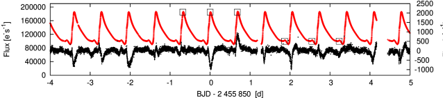
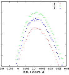
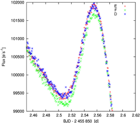
Figure 1: Cycle-to-cyle variation of the SC flux curve of NR Lyr. Top panel: a part of the flux curve around the pulsation maxima; middle panel: residual curve after we pre-whitened the data with 55 significant harmonics of the main pulsation frequency (right scale, black points) and for comparison the original flux curve (left scale, red points); bottom panels: three consecutive cycles from the flux curve signed by different colours and symbols folded to the cycle ‘B’ and ‘E’, respectively. The small boxes in the middle panel indicate the positions of these flux curve parts.

3.1 Cycle-to-cycle variation of the light curves

First we examined the SC time series. We used the raw flux data obtained from our tailor-made aperture photometry, which is practically a simple pixel flux value summation without any further processing.

While checking the flux curves we realised that the pulsation cycles are different to each other. As an example we show a part of the SC light curve of NR Lyr in Fig 1. The top panel shows the light curve around maxima of 13 consecutive pulsation cycles. The most striking feature is the different height of maxima. We marked three consecutive pulsation cycles with the letters ‘A’, ‘B’ and ‘C’. In the bottom left panel, the same three cycles are plotted by shifting ‘A’ and ‘C’ cycles to the position of ‘B’ (red plus), i.e. ‘A’ is shifted in the positive direction (blue asterisk) and ‘C’ is shifted in the negative direction (green x). As we can see, all the maxima are well-covered by observations and differ to each other significantly. The difference between maxima ‘B’ and ‘C’ is $\sim 1500$ e^-s^-1 (in magnitude scale is around 0.008 mag) which is huge compared to the observational error of individual data points ($\sim 2\times 10^{-5}$ mag).

Although the most striking feature is the different maxima, other parts of the light curves are also different. Looking at the three consecutive cycles marked with ‘D’, ‘E’ and ‘F’ in the top panel of Fig 1. The height of maxima of these cycles are almost the same, while cycle ‘F’ is a bit higher. Shifting the cycles ‘D’ (blue asterisk) and ‘F’ (green x) with plus or minus one pulsation cycle to the position of the cycle ‘E’ (red plus) and crop around the bumps (pulsation phase $\phi\sim 0.6-0.8$), we get the bottom right panel of Fig 1. We see that the light curves of cycles ‘D’ and ‘E’ are overlapped but cycle ‘F’ goes bellow these two. The difference is abut 300 e^-s^-1 (0.003 mag). Since cycle ‘F’ has the largest maximum amongst these three cycles there is no vertical shift which could eliminate both the maximum and the minimum differences simultaneously.

The complex structure of the light curve changes can be studied in detail by preparing the residual flux curve. A 55-element harmonic fit was removed from the data. The resulted curve is shown in the middle panel of Fig. 1 (black dots) with the original flux curve (red dots). The residual shows sharp spikes at around the light curve maxima. These spikes are positive or negative according to that the certain cycle flux curve is above or below the fit, respectively. Spikes can also be found at different phases than maxima ($\phi=0$). These phases are $\phi\sim 0.92,0.95,0.7,0.75$, and 0.1. The first two phases are the beginning and the end of the light curve feature of the ascending branch often called ‘hump’ while $\phi\sim 0.75$ is the position of the ‘bump’. The light curve of NR Lyr shows no evident features at the positions of $\phi\sim 0.7$ and 0.1 but these phases are the same that were defined by Chadid et al. (2014) as the positions of ‘rump’ and ‘jump’ recently. Maxima and these phases are those parts of the light curves where the most prominent shock waves are generated (Simon & Aikawa, 1986; Fokin, 1992; Chadid et al., 2008; Chadid & Preston, 2013).

We found similar cycle-to-cycle (hereafter C2C) variations for all stars which are brighter than $K_{\mathrm{p}}\sim 15.4$ mag (see ’yes’ sign in the fourth column of Table 2). The KIC $K_{\mathrm{p}}$ magnitudes given in Column 2 of Table 2 were determined by ground-based photometry by Brown et al. (2011), who observed each star in three different epochs. This observing strategy is well-suited to constant stars but it could result in inaccurate average magnitudes for large amplitude variable stars as RR Lyrae. The brightness of our stars are, therefore, better characterized by the measured average flux (Col. 3 in Table 2) than the KIC magnitudes.

The maximal brightness deviations is similar for all stars: the difference between the highest and lowest maxima is about 0.006-0.008 mag. This general value might be responsible for the lack of C2C variation of fainter stars: the higher observation noise make the effect to be undetectable. The situation is illustrated with Fig. 2 where we plotted the residual of the normalized flux ($F/\langle F\rangle$, where $F$ means the flux in e^-s^-1 and $\langle F\rangle$ is the average flux) curves of three stars with different brightness in the same scale. While the C2C variations of FN Lyr ($K_{\mathrm{p}}=12.88$ mag) in top panel of Fig. 2 is very similar to NR Lyr, the spikes are less detectable for the fainter KIC 6100702 ($K_{\mathrm{p}}=13.46$ mag, middle panel). Finally, no structure can be recognized within the higher noise level of the faintest star V368 Lyr ($K_{\mathrm{p}}=16.00$ mag, bottom panel).

The C2C behaviour of NR Lyr showed in Fig. 1 is typical not just in its amplitude but in its other characteristics as well. The difference in maxima are generally higher than the minima (or other parts of the light curves). The maxima (and minima) value variation seems to be random. Sometimes increasing or decreasing amplitude cycles follow each other but in many other cases a small amplitude cycle follows a large amplitude one or vice versa (see also top panels of Fig 1 and Fig 2).

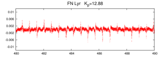
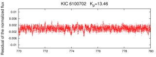
Figure 2: Ten-days-long parts of residual flux curves. The three different brightness stars are shown in the same relative scale. The apparent brightness of the stars are decreasing from top to bottom. The detectability of the C2C variation features are highly depends on the brightness. The fainter of the star the hardest to detect the effect.

Table 2: Detection of the C2C variation. Name; Kepler $K_{\mathrm{p}}$ brightness from the KIC catalogue (Brown et al., 2011); C2C variation detection by eye; Detection index $D$ (see the text for the details).

Name	$K_{\mathrm{p}}$	$\langle F\rangle$	C2C	$D_{5}$
	(mag)	e-s-1
NR Lyr	12.684	128717	yes	69.8
V715 Cyg	16.265	4731		14.5
V782 Cyg	15.392	12892	yes	35.7
V784 Cyg	15.370	10129	?	76.2
KIC 6100702	13.458	48145	yes	92.9
NQ Lyr	13.075	63394	yes	98.7
FN Lyr	12.876	115746	yes	96.6
KIC 7030715	13.452	76707	yes	112.8
V349 Lyr	17.433	1638		21.0
V368 Lyr	16.002	3772		21.6
V1510 Cyg	14.494	19762	yes	28.2
V346 Lyr	16.421	2404	?	28.2
V894 Cyg	13.293	91854	yes	109.8
KIC 9658012	16.001	6692	yes	26.8
KIC 9717032	17.194	2521		11.6
V2470 Cyg	13.300	64935	yes	114.3
V1107 Cyg	15.648	6293	yes	34.0
V839 Cyg	14.066	25339	yes	32.0
AW Dra	13.053	108385	yes	95.4

3.2 Origin of the C2C variations

Although Chadid (2000) and Chadid & Preston (2013) reported spectroscopic C2C variations of RR Lyrae stars, on ground-based photometric basis only marginal signs of such an effect were published (e.g. Barcza 2002; Jurcsik et al. 2008). On space photometric basis no similar C2C variation of non-Blazhko RRab stars have been reported ever before, so we checked our finding carefully.

(i) It is known that disruptions such as safe modes, the regular monthly downloads of data or quarterly rolls could cause abrupt changes in the row Kepler fluxes (Fanelli et al., 2011). We indeed detected small flux curve changes for many stars after such events but the C2C variations are appeared continuously over the entire data sets and are not concentrated around the discontinuity events. This rules out that the C2C variations would result from this technical problem.

(ii) To avoid possible data handling problems which may cause such an effect we used the raw tailor-made aperture photometric fluxes. The local instrumental trends were handled in three different ways. (1) For 13 stars the SC data show no serious instrumental trends so we used these data without any further processing. (2) The raw data of six stars, however, show noticeable trends which were removed by subtraction of fitted polinomials. (3) As an independent check we applied a method to all SC data sets in which we adjust each pulsation cycle to a common zero point. For a given star a Fourier sum was fitted to each cycle separately, the determined zero points were connected with a smooth continuous curve which was then subtracted from the data. This algorithm works well and removes the tiniest instrumental trends but it has an assumption that zero point variations can only be caused by instrumental effects. Although no systematic amplitude changes connected to this small zero point corrections were detected in any of the studied stars, it is known that, for example, the Blazhko effect also causes zero point variations (Jurcsik et al., 2005, 2006, 2008). In this respect, we know nothing about the C2C variations, so we did not use these zero point corrected data except for this test.

We compared the C2C variations of the raw (1) or the globally corrected (2) data to the zero point corrected (3) data. These comparisons resulted in qualitatively similar C2C variations though the actual value of the quantitative properties (e.g. amplitude difference between consecutive cycles) was slightly different. This test showed that the C2C variation is not caused by our data handling.

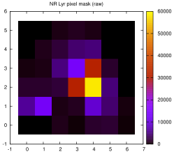
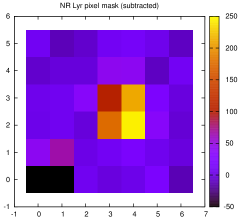
Figure 3: The pixel mask of NR Lyr during the SC (Q11.1) observation. The upper panel shows the flux in ‘high’ maximum signed by ‘C’ in Fig. 1, while the lower panel contains the flux difference of the ‘high’maximum ‘C’ and ‘low’ maximum ‘B’.

(iii) The next potential cause can come from the photometry, such as background sources, drift of the stars in the CCD frame, etc. We have chosen high and low maxima pairs from the light curves and plotted the flux in the pixel maps at the high maximum phase and also the flux differences between the high and low maxima phases. This is plotted for NR Lyr in Fig. 3. The figure shows that (1) the amplitude difference is connected to the star and there is not any other sources of light and (2) the position of the star is fixed within the pixel mask. These image properties minimize the chance of C2C variations being caused by serious photometric problems.

The investigation of the pixel masks resulted in a by-product. We found a faint variable source in the frame of V784 Cyg. The source was identified with the star KIS J195622.44+412013.9 ($g=20.19$, $r=19.32$ and $i=18.67$ mag) observed by the Kepler-INT survey (Greiss et al., 2012) (see also last paragraph in Sec 4.2). Other variable sources have not been found in any other frames.

(iv) For testing unknown instrumental effects as an explanation of C2C variation, we investigated similar observations with a different instrument. Currently the only independent instrument which observed high precision time series for non-Blazhko RR Lyrae stars is the CoRoT space telescope (Baglin et al., 2006). To our knowledge three non-Blazhko stars were observed with the oversampled mode which mean 32 sec sampling. (The time coverage of the normal 8 min sampling of CoRoT is too sparse for our porpose.) These are: CoRoT 103800818 (r${}_{\mathrm{CoRoT}}=14.39$ mag, Szabó et al. 2014), CM Ori (CoRoT 617282043, r${}_{\mathrm{CoRoT}}=12.64$ mag, Benkő et al. 2016) and the BT Ser (CoRoT 105173544, r${}_{\mathrm{CoRoT}}=12.99$ mag) which was overlooked by previous CoRoT RR Lyr studies.

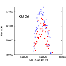
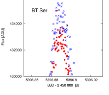
Figure 4: The amplitude difference of consecutive cycles in CoRoT non-Blazhko stars. The red dots mean the original light curve points while the blue ‘x’ symbols show the light curve points shifted one pulsation cycle.

We used the oversampled flux time series of CoRoT 103800818 from LRc04 run (74.6 d long oversampled part, 176 871 data points), CM Ori LRa05 (90.5 d, 200 999 observations), and BT Ser which was observed in two subsequent CoRoT runs LRc05 and LRc06, meaning 168.4 d-long almost continuous observations with 391 455 individual data points. These amount of data are comparable with the SC data of present Kepler sample. CM Ori and BT Ser are relatively bright: despite the smaller aperture of CoRoT we have similarly accurate light curves for these stars as for the fainter Kepler stars.

We performed similar investigation of the CoRoT light curves as we did for Kepler stars and we found C2C variation for the two brighter stars CM Ori and BT Ser. Fig. 4 shows their amplitude variation in the same way that was plotted in the bottom left panel of Fig. 1 for NR Lyr. Even though the scatter is evidently higher, the amplitude difference is obvious. The largest difference between high and low amplitude maxima is about 0.005-0.006 mag. This value is similar to our estimation obtained from Kepler stars. The $\sim$2 mag fainter third star CoRoT 103800818 show no C2C variation as we expected on the basis of Kepler sample where also seems to be exist a detection limit at about 15.4 mag.

These tests suggest that the detected C2C variations are predominantly belong to the stars. Of course, serious time- and flux-dependent non-linearity of the detectors might cause similar effects, however, no such problems have been reported neither for CoRoT nor for Kepler. A promising independent check opportunity will be the analysis of TESS (Ricker et al., 2015) oversampled (2-min) data.

(v) There is an additional argument that the C2C light curve variations belong to the stars: the shape of the residual light curves. The spikes described in Sec 3.1 are not randomly distributed in the pulsation phase but appeared exactly at the phase of the hydrodynamic shocks. This findings argees well with the results of radial velocity studies (Chadid, 2000; Chadid & Preston, 2013) where the C2C radial velocity curve variations were explained cycle to cycle variation of the hydrodynamic phenomena induced the shock waves in RR Lyrae atmosphere.

3.3 Characterising the C2C variations

Beyond the visual inspection done in Sec. 3.1, we defined a quantity which numerically measures the detectability of the C2C variations. As we have seen the C2C variations focus around the pulsation maxima therefore the residual flux curves show spikes around these positions (Fig. 2). The phase diagrams of these residual flux curves show a broadening around the phase of the pulsation maxima ($\phi=0.5$ see Fig 5). By comparing the amplitudes of these broadenings to the amplitude of non-broadened phases, we can define a numerical value wich typify the detectability of C2C variation.

A simple statistical approach was implemented. We folded the SC residual flux curves $r(t)$ with their periods then the obtained $r(\phi)$ phase diagrams were splitted into few bins: $r_{1},r_{2},\dots r_{n}$ ($n$ is integer). In each bin the average of the absolute values of the residual fluxes $\langle|r_{i}|\rangle$ and its standard error $s_{i}$ was determined. The difference between the maximal and minimal bin values is

$$\Delta_{n}:=\left[\langle|r_{j}|\rangle^{\mathrm{(max)}}-{\langle|r_{k}|\rangle^{\mathrm{(min)}}}\right],\ \ \ j,k\in{1,2,\dots,n}.$$ (1)

We can define the detectation parameter as

$$D_{n}:=\frac{\Delta_{n}}{s_{n}},\ \ \ {\mathrm{where}}\ \ \ s_{n}=\max(s_{j},s_{k}).$$ (2)

The $D_{n}$ is a significance-like parameter. It measures how much larger the average flux of the central bin which contains the spike than a bin which definitely not contains it. The difference is expressed in the ratio of the standard error. In column 4 of Table 2 the $D_{5}$ values are given. If a star has more than one distinct SC quarter observations, we determined $D$ for each quarter separately, and here we show their averages.

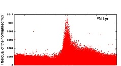
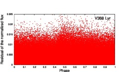
Figure 5: The absolute values of the residual of the normalized flux vs. phase diagram of FN Lyr (up) and V368 Lyr (down).

The $D$ seem to be good C2C variations detection indicator: if $D$ value is high ($D>30$) we can detect evident C2C light curve variations by eye and if this value is low ($D<25$) we cannot see anything. The faint variable in the frame of V784 Cyg disturbs the visual inspection, but the $D$ parameter clearly show the existence of the C2C variation. There is a trend between the parameter $D$ and the average flux $\langle F\rangle$ (Column 3 in Table 2): the brighter the star, the higher the associated $D$ parameter. It suggests that the phenomenon is similar in strength for all stars and the differences of the detection are mainly because of the brightness differences.

The C2C variations seem to be random. To investigate this, we prepared the Fourier amplitude and phase variation functions. The SC light curves were divided into period-long bins and so each bin contained abut 600-800 points depending on the cycle size. This handling minimize numerous possible technical problems such as zero point fluctuations or short time-scale trends. The amplitude and phase variation functions $A_{n}(t)$, $\phi_{n}(t)$ were calculated for each star by applying ten-element harmonic fits. This calculation has been done with the LCfit (Sódor, 2012) non-linear Fourier fitting package.

Plachy et al. (2013) investigated RR Lyrae models corresponding to resonance states and chaotic pulsation. Their synthetic chaotic luminosity curves show similar changes than we presented here: the random-like changes are concentrated around the maxima and the amplitudes are also in similar magnitude range. These raise the possibility that by the C2C variations we observed might be the sign of chaotic pulsation. Detailed testing of such a possibility is far beyond the goal of this paper but we investigated the Poincare return maps of $A_{1}$ and $\phi_{1}$ values as a fast and easy check. We prepared four maps for each star: $(A_{1}^{(j)},A_{1}^{(j+1)})$, $(A_{1}^{(j)},A_{1}^{(j+2)})$, $(\phi_{1}^{(j)},\phi_{1}^{(j+1)})$ and $(\phi_{1}^{(j)},\phi_{1}^{(j+2)})$. Here $j$ integers mean the cycle numbers of the pulsation. Most of these maps have an oval shape showing the amplitude and phase variations but no other evident structures can be detected. That is, the observed C2C variations might be chaotic but we cannot verify this at least with the return maps, certainly.

4 Fourier spectra

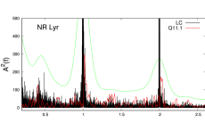
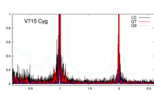
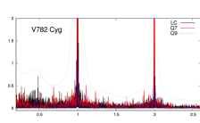
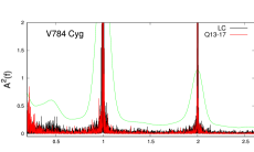
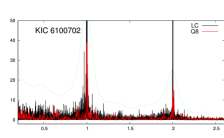
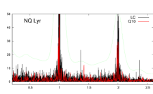
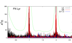
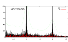
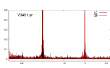
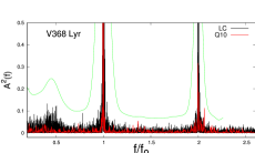
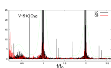
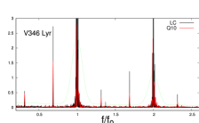
Figure 6: Power spectra of the residuals around the main pulsation frequency $f_{0}$ and its first harmonic 2$f_{0}$. Black curves show the LC power spectra. Spectra computed from the SC data are signed red and blue curves (for the actual quarter numbers see the labels in the panels). Providing comparable spectra we scaled the horizontal axes with the value of $f/f_{0}$. The vertical scales of SC power spectra are also normalized to the signal to noise ratio of the LC spectra. Dotted green curves show the estimated $S/N=4$ values of the LC spectra.

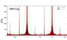
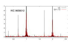
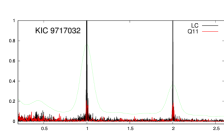
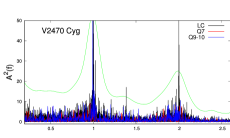
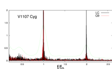
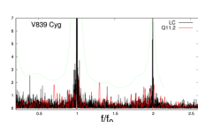
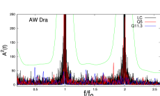
Figure 7: Continuation of Fig. 6

We prepared the Fourier spectra of both the LC and the SC light curves using the discrete Fourier transform tool of the program package MuFrAn (Kolláth, 1990). The spectra are dominated by the main pulsation frequencies $f_{0}$ and their harmonics $nf_{0}$ ($n$ is a positive integer). After pre-whitening the data for a significant number (35-55) of harmonics we obtainded the residual spectra. In Fig. 6-7 parts of the residual power spectra are shown around the main pulsation frequencies ($f_{0}$) and their first harmonics ($2f_{0}$). The black lines indicate the LC spectra, while the spectra of the SC light curves are shown with thin red lines. For those stars where two distinct SC observations are available (e.g. Q7 and Q9 for V715 Cyg, etc., see Table 1) the second SC spectra are plotted by dotted blue lines (see the labels in the panels).

The power spectra are vertically normalized with (in practice divided to) the signal-to-noise ratio S/N (Breger et al., 1993) of the LC spectra. The S/N=4 ratio functions of the LC data are plotted in green dotted lines in Fig. 6-7. Strictly speaking, the shape of the SC and the LC S/N ratio vs. frequency functions are different, so we cannot transform them to each other by a simple normalization but such a normalization can give an approximate agreement in a shorter frequency interval. That is, the S/N ratio of the LC spectra is approximately valid for all spectra within the $f_{0}$ and $2f_{0}$ intervals plotted in the panels. The noise level around the harmonics are overestimated because of the instrumental origin side peaks appearing in the LC spectra (see fig. 4. in Benkő et al. 2019). Instead of the frequency, the horizontal axes show the $f/f_{0}$ values because this way the spectra can be compared directly.

4.1 Signs of the C2C variations

How does the Fourier spectrum of a randomly C2C varying light curve residual look like? In order to check this, we prepared synthetic light curves, for which we used the formulae of simultaneous amplitude and frequency modulation summarised in Benkő et al. (2011); Benkő (2018). The carrier wave coefficients (frequency, harmonic amplitudes and phases) defined a simplified RR Lyrae-like light curve with nine harmonics, and C2C randomly changing amplitude modulation functions for both amplitude and frequency modulation parts were assumed. The random values were set for each amplitude and phase separately. The synthetic light curves were sampled in the same points as the observed Q7 SC data. The spectra of the synthetic light curves after we removed the nine harmonics from the data show significant peaks at the first few (4-5) harmonics. The surroundings of the peaks have a red noise profile as we expected from a random process.

Comparing these synthetic spectra with the spectra of the observed SC data, we found them fairly similar. The observed SC residual spectra are also dominated by frequencies at around $f_{0}$ and its harmonics. This is true for the entire sample not just for the bright stars which show evident C2C variations and high $D$ values but for the faintest stars as well. The high-$D$ stars show many ($>10$) significant harmonic peaks while low-$D$ stars have typically few (3-4) significant harmonics. This can be explained with that the fine structure of the spikes at the higher harmonics are veiled by the higher noise of low-$D$ stars. For most cases we detect more than one single peak around the harmonic positions $kf_{0},k=1,2,\dots$ which is again a similarity to the synthetic data spectra. These side peaks due to the C2C variation might explain the distinct group with extremely small Blazhko amplitude found by Kovács (2018). Double or multiple peaks, however, could not be just because of the C2C variations. This can also be the consequences of long time-scale (longer than the observed time span) light curve variations caused by instrumental problems or very long period Blazhko effect. Since we found some evidence for such effects (see later in Sec. 5.1), we cannot declare undoubtedly the detection of the C2C variations on all stars. This also means that the Fourier spectra alone are not discriminative enough to find C2C variations.

4.2 Additional modes

Six stars’ LC spectra show significant ($S/N>4$) additional peaks around the main pulsation frequency and its first harmonics. These are: NQ Lyr, V1510 Cyg, V346 Lyr, V894 Cyg, KIC 9658012 and V2470 Cyg. SC spectra of three of these stars (V346 Lyr, V894 Cyg and KIC 9658012) contain significant additional frequencies. Several other stars show visible but strictly not significant (2$<$S/N$<$4) peaks in their LC or SC spectra. The frequency of the highest additional peaks with their S/N ratio are given in Table 3.

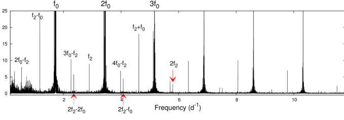
Figure 8: A possible identification of the additional mode frequencies in the pre-whitened spectrum of the LC light curve of V1510 Cyg. The positions of the main pulsation frequency and its first two harmonics are also marked.

In the past years low amplitude additional frequencies were found for many RR Lyrae stars (for a resent review see Molnár et al. 2017). If we focus only on the fundamental mode pulsators (RRab stars) then the half-integer frequencies ($f_{0}/2,3f_{0}/2,\dots$) of the period doubling (PD) effect (Kolenberg et al., 2010; Szabó et al., 2010) appearing in many Blazhko RRab stars was the first theoretically modelled case. Other type of extra frequencies which were discovered in numerous Blazho RRab stars are the low order radial overtone frequencies ($f_{1},f_{2}$ Chadid et al. 2010; Poretti et al. 2010; Benkő et al. 2010) and their linear combinations with the fundamental mode frequency. Although the simultaneous appearing of the PD and the first overtone frequencies was reproduced by radial numerical hydrodynamic codes as triple resonance states (Molnár et al., 2012), it is not evident that all of such frequencies can be explained on this purely radial basis. Especially thought-provoking that the amplitude of the ‘linear combination’ frequencies are many times higher than their suspected basis frequencies. Such a behaviour is detected for nonradial modes empirically for rhoAp stars by Balona et al. (2013) and explained by theoretically Kurtz et al. (2015) which suggests that these frequencies could belong to non-radial modes excited at or near the radial mode positions.

The extra frequencies of V1510 Cyg, V346 Lyr, V894 Cyg and KIC 9658012 could be identified as the second radial overtone mode $f_{2}$ and their linear combinations. This identification are shown in Fig. 8 for V1510 Cyg which has the richest extra frequency pattern. As we see, a few linear combination frequencies (e.g. $f_{2}-f_{0}$, $f_{2}+f_{0}$, or $3f_{0}-f_{2}$) have an amplitude higher than the amplitude of $f_{2}$. The situation is the same for V346 Lyr and V894 Cyg: the highest amplitude extra frequency is $f_{2}-f_{0}$, while for KIC 9658012 it is the $f_{2}$. Stars where the highest amplitude additional frequency is lower than the fundamental one are rather rare. We found V838 Cyg (Benkő et al., 2014) the only published case. Additional mode frequencies at the position of $f_{2}-f_{0}$ are known for few CoRoT and Kepler Blazhko RRab stars (see Benkő & Szabó 2014 and references therein) but in all those cases the frequency $2f_{2}-2f_{0}$ has higher amplitude.

On the basis of their additional frequency content NQ Lyr and V2470 Cyg form a separate subgroup in our sample. Their highest additional peaks are around the position of the first radial overtone frequency $f_{1}$, but their frequency ratios ($f_{0}/f_{1}=0.732$ for NQ Lyr and 0.722 for V2470 Cyg) are lying bellow the values of the canonical Petersen diagram. Such ratios have been detected for the first time for two RRd stars in the globular cluster M3 by Clementini et al. (2004). Later similar ratio has been found for the Kepler Blazhko RRab stars V445 Lyr (Guggenberger et al., 2012) and RR Lyr itself (Molnár et al., 2012). In the OGLE survey data of the Galactic Bulge has been found numerous RRd stars showing similarly small frequency ratios (Soszyński et al., 2011, 2014). Studying the RRd stars in the globular cluster M3 Jurcsik et al. (2014, 2015) found that all four Blazhko RRd stars have anomalous frequency ratio and three of them have smaller then the normal one as we found for the present stars. Significant amount of such RRd stars were identified in the Large Magellanic Cloud by the OGLE survey (Soszyński et al., 2016) and also in K2 data (Molnár et al., 2017).

Soszyński et al. (2016) defined these stars as ‘anomalous double-mode RR Lyrae stars’. This group is characterized by not just its anomalous period (or frequency) ratio but the dominant pulsation mode is the fundamental one here while for the ‘normal’ RRds it is the first overtone. Additionally, most of these anomalous RRd stars show the Blazhko effect (Smolec et al., 2015). Since we analyzed RR Lyrae stars classified formerly as RRab type it is evident that NQ Lyr and V2470 Cyg is dominated by the fundamental mode. The amplitude ratios are $A(f_{1})/A(f_{0})=0.00025$ and 0.00032 for NQ Lyr and V2470 Cyg, respectively. These ratios are two-three magnitudes smaller than the similar parameters of the anomalous RRd stars discovered from the ground (Jurcsik et al., 2014; Soszyński et al., 2016). The anomalous RRd stars almost always show the Blazhko effect. However, we did not detect any modulation for our stars (see the details later). Of course, very small amplitude and very long period (longer than four years) modulation can not be ruled out.

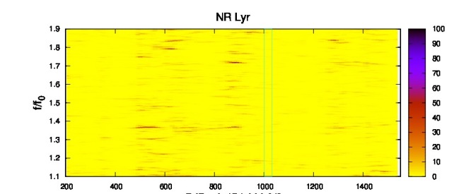
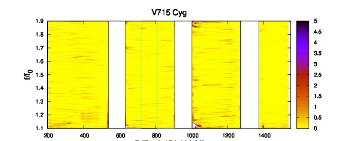
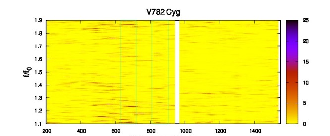
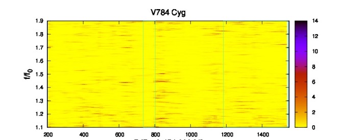
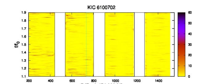
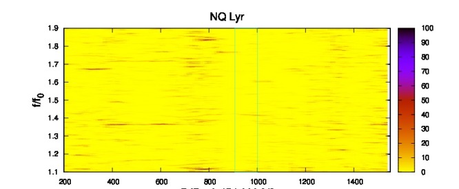
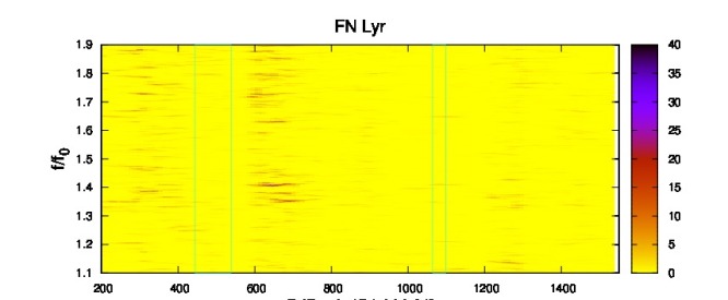
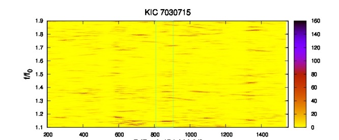
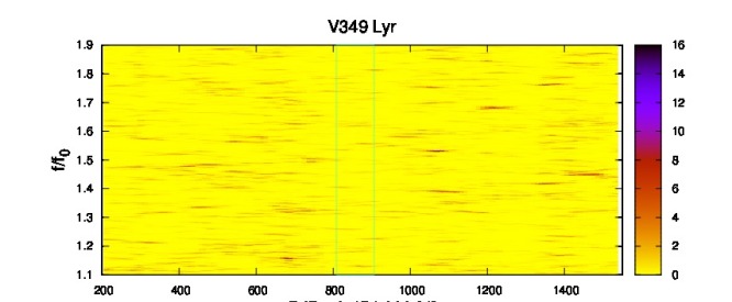
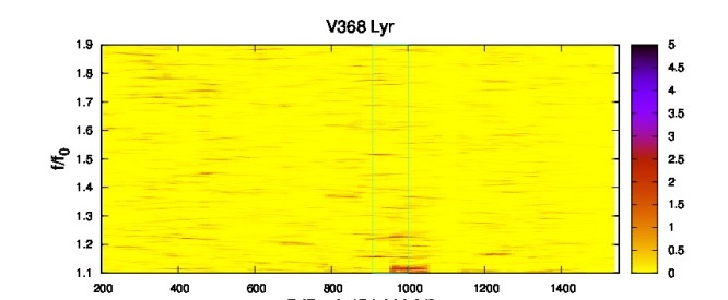
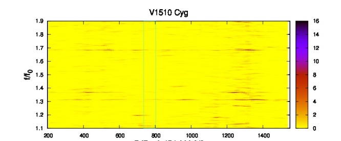
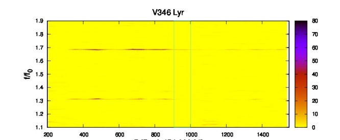
Figure 9: Time-frequency variation of the frequencies around the main pulsation frequency $f_{0}$ and its first harmonic 2$f_{0}$. Showing comparable spectra we indicated the normalized frequency $f/f_{0}$ in the horizontal axes.

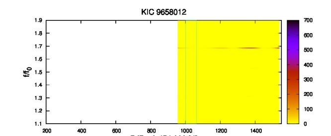
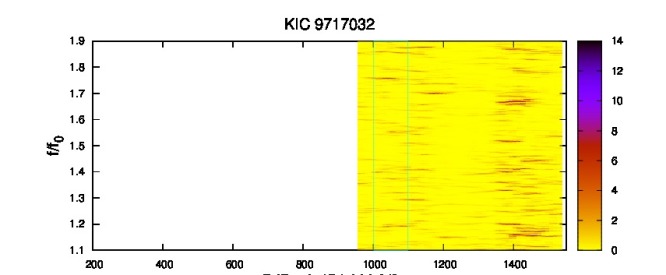
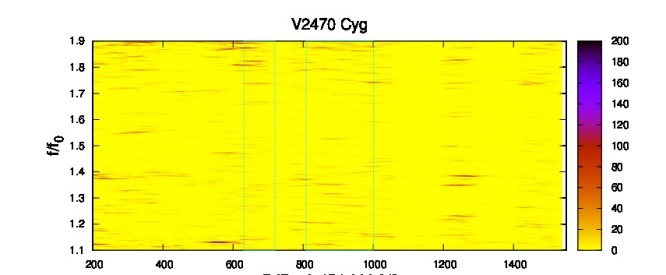
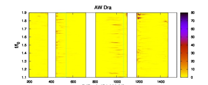
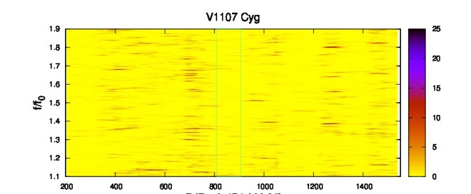
Figure 10: Continuation of Fig. 9.

As Clementini et al. (2004) and Soszyński et al. (2011, 2016) pointed out the low frequency ratio of anomalous RRd stars could only be obtained from the evolutionary models assuming either higher metallicity ([Fe/H]$>-0.5$) or smaller mass ($M<0.55$ M_☉) than the usual parameters of RR Lyrae stars. For the Kepler sample metallicities from high resolution spectroscopy were published by Nemec et al. (2013). They found the metallicity of NQ Lyr and V2470 Cyg to be [Fe/H]$=-1.89\pm 0.10$ dex and [Fe/H]$=-0.59\pm 0.13$ dex, respectively. Comparing these values with the period ratios we can conclude that the standard evolutionary theory cannot explain neither of these stars’ present position in the instability strip (see fig. 8 in Chadid et al. 2010). It needs an alternate evolutionary channel as it was suggested by Soszyński et al. (2016). Since the mass seems to be lower than the normal RR Lyrae regime we raise the possibility that this altenate tracks could belong to binaries similarly to the case of OGLE-BLG-RRLYR-02792 (Smolec et al., 2013). This idea can be justified or refuted by a future spectroscopic work. Alternatively Plachy et al. (2013) found higher order resonant solutions in their hydrodynamic codes (e.g. with 8:11, or 14:19 ratios between $f_{0}/f_{1}$) which frequency ratios are outside the traditional RRd range but very similar to the ratio of the observed anomalous RRd stars. In this case the mass and metallicity are not necessary anomalous.

We detected in many SC and/or LC spectra an increase around the half of the main pulsation frequency ($\sim f_{0}/2$). In some cases distinct visible but not really significant peaks ($S/N<4$) are also appear (see e.g. NR Lyr, V782 Cyg) around $0.48-0.49f_{0}$ but in most cases only the noise level increases around this position. It is shown well by the S/N ratio curves (green dotted lines in Fig. 6-7). The reason of this feature is not clear. Some possible explanations: (i) There is a rough trend within the signs of the residual light curve peaks: a positive peak is followed by a negative and vice versa. If this effect would be more regular we would seen a kind of ‘period doubling’ and its Fourier representation would be the subharmonic $kf_{0}/2$ frequencies. However, we can see in Fig. 1 and 2 that this feature are far from the regularity and for all observed PD effect the highest amplitude frequency is the $3f_{0}/2$ and not $f_{0}/2$ as we see here. (ii) The frequencies of the increase around $\sim f_{0}/2$ could be linear combination frequencies as $f^{\prime}-f_{0}$. In this scenario $f^{\prime}$ frequencies would be located around the first overtone $f_{1}$ with anomalous frequency ratio ($\sim 0.72-0.73$). This way, almost all RRab stars would show anomalous RRd behaviour. (iii) The formerly cited work of Plachy et al. (2013) investigated the Fourier spectra of synthetic luminosity curves belongs to e.g. 6:8 resonance solutions. These models show similar subharmonic structures (see their fig. 8) what we presented here but our light curves do not show any other signs of this resonance. Higher order hardly detectable resonances might also explain the phenomenon but this scenario is rather speculative. (iv) No less than the assumption in which non-radial g modes are assumed as an explanation. The frequency range of the detected increases are bellow the Brunt-Väisälä frequency but calculations for non-radial modes of RR Lyrae stars did not obtain considerable amplitudes around these regions (Van Hoolst et al., 1998; Nowakowski & Dziembowski, 2003; Dziembowski, 2016). Therefore, this spectral feature requires further observational and theoretical investigations.

Finally we note, that we found a significant peak of V784 Cyg spectrum at 10.1393454 d^-1 ($S/N=7.1$). The frequency must belong to the background star KIS J195622.44+412013.9 which was mentioned in Sec. 3.2 because such a frequency would be very unusual for an RR Lyrae star and it has no linear combination with the pulsation frequency of V784 Cyg. This frequency is typical of a $\delta$ Scuti star, suggesting the variability type of KIS J195622.44+412013.9.

4.3 Time frequency variations

All the detected additional frequencies show noticeable time dependency. The relative amplitude of the peaks are different for different time spans (LC, SCs) even so some peaks are undetectable in a given time series. Some frequency changes can also be suspected.

Time frequency analysis tools such as wavelet or Gabor transformations generally need strickly equidistant time series. So the observed data must be interpolated somehow. Avoiding this, we chose the simple time dependent Fourier tool of the SigSpec (Reegen, 2007, 2011) package. As inputs we used the LC light curve residuals which were obtained after removing 55-harmonic Fourier fits from the original light curves. We set in SigSpec one hundred days-long time bins for each star and used ten-day steps. This resulted in $\sim 150$ Fourier spectra for each target.

Since additional peaks appear between $f_{0}$ and $2f_{0}$, we show this area of the spectra in Figs. 9 and 10 as contour plots. For easier comparison, instead of the frequencies in the vertical axes, similar to the Figs. 6 and 7, the quantity $f/f_{0}$ is indicated. The colour scales show the power values. The white area in panels indicate the missing data quarters when the given stars were located in any of the corrupted chips. The green boxes symbolise the time spans of the SC observations.

Figs. 9 and 10 illustrate how the amplitudes of the additional frequencies dynamically change. Similar amplitude changes were revealed for the additional modes of Blazhko RRab and RRc stars (Benkő et al., 2010; Szabó et al., 2010, 2014; Moskalik et al., 2015). The SC spectra in Figs. 6-7 represent snapshots of these variations. This explains the sometimes different frequency content of the SC and LC spectra. It is well traceable e.g. how the amplitude of $3f_{0}-f_{2}$ of V894 Cyg decreased from a significant level to below the detection limit from the beginning of the observations to the time of the SC quarter.

The figures allow us to find such additional frequencies which are significant only in a short time interval not observed any of the SC quarters and averaged out from the spectra of the four-years LC data. The detected frequencies with their approximate visibility dates in the brackets are the followings: NR Lyr: $f_{1}$ ($t\sim 450-850$ d), and $f_{2}$ ($t\sim 900$ d); KIC 6100702: $f_{1}$ ($t\sim 200-400$ d); NQ Lyr: $f_{2}$ ($t\sim 300-400$ d); FN Lyr: $f_{1}$ ($t\sim 650$ d). Three of these stars (NR Lyr, KIC 6100702 and FN Lyr) do not show significant additional modes in their SC and LC spectra.

4.4 Connection between the C2C variations and the additional modes

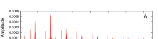
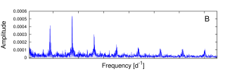
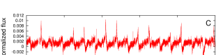
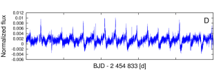
Figure 11: The role of the additional frequencies in C2C variations. Residual spectrum of the nomalized SC flux curve of V894 Lyr (panel A) and the same spectrum if we pre-whitened the additional frequencies from the data (panel B). Part of the residual SC flux curve (panel C) and the same flux curve part after we removed the additional frequencies (panel D).

In the case of previously studied regular C2C light curve variations of the Blazhko stars as period doubling (Kolenberg et al., 2010; Szabó et al., 2010) or other resonances (Molnár et al., 2012, 2014) suggest that the extra modes which manifest additional frequencies in the Fourier spectra, can cause regular C2C variations on the light curves.

Taking these into account, the question arises: what is the relationship between the observed extra frequencies and the C2C variation? First, there are a number of stars which (e.g. V782 Cyg, KIC 6100702, KIC 7030715, AW Dra) show significant C2C variations but there are no signs of any additional mode frequencies in their SC spectra. In other words, the excited additional modes can be ruled out as the only reason of the C2C variation.

Second, we tested the role of the additional modes in the C2C variation. For this, we used the stars with additional modes (V346 Lyr, V894 Lyr and KIC 9658012), pre-whitened all the significant additional frequencies and their linear combinations from their light curve, then we re-analysed them searching for C2C variations in the same way as in Sec. 3.1 for the original curves. We only show the results of V894 Lyr which is the brightest among these three stars. Fig. 11 shows the spectra before (panel A) and after (panel B) pre-whitening the additional frequencies from the data. Because of the time dependent amplitudes discussed in Sec. 4.3, some frequencies remain after the pre-whitening process but with marginal amplitudes. The normalized flux curves belonging to these spectra are shown in the panels C and D. The flux curves with and without removing the additional frequencies have very similar shapes illustrating that the additional modes only marginally affect the C2C variations. The dominant random variation seems to be independent from these modes.

5 The presence of the Blazhko effect

The present hypothesis is that amongst RRab stars only the Blazhko stars show additional frequencies. This hypothesis was set because sooner or later all the non-Blazhko stars showing additional modes turned out to display the Blazhko effect (Benkő et al., 2010; Nemec et al., 2011; Benkő & Szabó, 2015). In the previous section, however, we have seen that considerable part of the Kepler non-Blazhko sample shows additional mode pulsation. This is true even if we omit the discovered anomalous RRd stars from the sample.

The presence or the lack of the Blazhko effect needs a careful investigation. It is especially relevant now, because a recent result suggests that the Blazhko incidence ratio among RRab stars could be as high as 90% (Kovács, 2018).

5.1 The O$-$C diagrams

The Blazhko effect means simultaneous amplitude and frequency/phase modulation with the same frequency or frequencies. If the amplitude of the amplitude modulation part is high enough this effect can be easily detected. This is obviously not true for our sample. The amplitude modulations if they exist at all must be of very low amplitude. In addition, the amplitudes are more sensitive to the instrumental and data handling problems than the phase, therefore the potential phase variations were carefully tested by using a refined version of the classical O$-$C (observed minus calculated) method (Sterken 2005 and references therein).

Traditionally, the O$-$C diagrams are constructed from definite phase points of a periodic light curve (maxima, minima, etc.). The exact position of these phase points (the ‘O’ values) are determined by the e.g. maxima of a least square fitted polynomial, or spline function around the predicted (‘C’) positions. As Jurcsik et al. (2001) showed for the sparse data of globular cluster $\omega$ Cen RR Lyrae the accuracy of O$-$C diagrams can be significantly improved if we define a template and the ‘O’ values are determined from the least square minimization of the horizontal shifts of the template at each proper position. This way we take into account the entire light curve and not just parts of it around the critical phases. This method was applied by Derekas et al. (2012) when they detected the random period jitter of a Cepheid (V1154 Cyg), and also by Li & Qian (2014) and Guggenberger & Steixner (2015) who search for potential light-time effect caused by a companion in the Kepler RR Lyrae sample. This work used the same implementation of the method what we used in Benkő et al. (2016), namely the program of Derekas et al. (2012) sligthly adjusted to RR Lyrae stars.

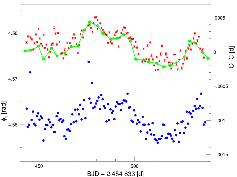
Figure 12: O$-$C variation of the SC data of AW Dra in the Kepler Q5 quarter (red squares with errorbars) with the parallel phase variation $\phi_{1}(E)$ (blue dots) where we transformed the time variation into epoch scale. The green astrisks connected with straight lines show the O$-$C values calculated from the LC data (see the text for the details).

O$-$C diagrams were constructed for both the SC and the LC light curves. In the case of the SC data each pulsation cycle can be handled separately without any problems, however, it does not work for the LC data due to their sparse sampling. For the LC light curves five-cycle-long parts were chosen and the template shift values (viz. the ‘O’ values) were determined on these intervals. This handling means an averaging which smooths the O$-$C curve but proved to be a good compromise. When we leave the cycle-by-cycle handling we lose only a little information as it is demonstrated in the upper curve of Fig. 12 but we win a much longer data set. The green continuous line in Fig. 12 shows the O$-$C diagram of the LC data calculated with this manner. As we seen the O$-$C diagrams of the LC data handling by our method are sufficient ever for studying rather short time scale variations as well. Accordingly, unless otherwise stated, we describe here the results obtained from the LC data.

Table 3: Some parameters of the sample stars. ID; period published by Nemec et al. (2013) $P_{\mathrm{N}}$; improved period $P_{0}$; period change rate $\dot{P}$, and its accuracy; the highest amplitude additional mode frequency, its possible identification and signal-to-noise ratio. The given number of digits of the periods and the frequencies indicate the accuracy.

ID	$P_{\mathrm{N}}$	$P_{0}$	$\dot{P}$	$\sigma(\dot{P})$	Add. fr.	$S/N$
	(d)	(d)	$\times 10^{-10}$	$\times 10^{-11}$	(d-1)
NR Lyr	0.6820264	0.6820268	12.38	6.98
V715 Cyg	0.47070609	0.4707059	$-$15.13	4.29
V782 Cyg	0.5236377	0.5236375	4.50	3.21
V784 Cyg	0.5340941	0.5340947	$-$4.51	3.6
KIC 6100702	0.4881457	0.4881452	$-$1.24	2.56
NQ Lyr	0.5877887	0.5877889	$-$8.43	3.94	$2.323822=f_{1}$	4.2
FN Lyr	0.52739847	0.5273986	$-$9.31	3.78
KIC 7030715	0.68361247	0.6836125	4.58	8.16
V349 Lyr	0.5070740	0.5070742	0.41	5.90
V368 Lyr	0.4564851	0.4564859	$-$11.81	2.67
V1510 Cyg	0.5811436	0.5811426	27.41	5.41	$1.178286=f_{2}-f_{0}$	7.6
V346 Lyr	0.5768288	0.5768270	12.40	20.41	$1.189183=f_{2}-f_{0}$	13.3
V894L̇yr	0.5713866	0.5713865	22.66	14.24	$1.198871=f_{2}-f_{0}$	9.5
KIC 9658012	0.533206	0.533195	$-$7.87	36.08	$3.164672=f_{2}$	11.0
KIC 9717032	0.5569092	0.556908	74.14	39.43
V2470 Cyg	0.5485905	0.5485897	$-$1.21	3.11	$2.524809=f_{1}$	4.1
V1107 Cyg	0.5657781	0.5657795	$-$0.40	5.76
V839 Cyg	0.4337747	0.4337742	1.39	6.45
AW Dra	0.6872160	0.6872186	$-$53.39	18.26

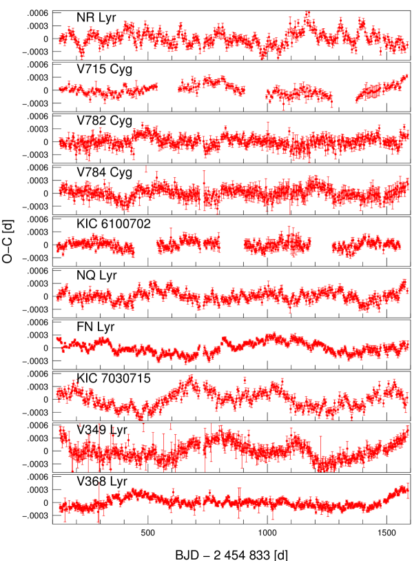
Figure 13: O$-$C diagrams of the LC data after removing a linear and a quadratic trends (in the left). The Fourier spectra of the left-hand-side O$-$C diagrams (in the middle) and these spectra after we removed the detected instrumental frequencies connected to the Kepler year (in the right).

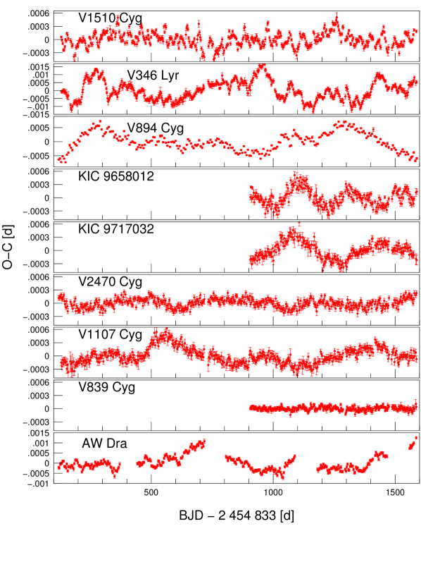
Figure 14: Continue of Fig. 13. We call the attention the O$-$C diagrams of three stars (KIC  8344381, KIC 9591503 and KIC 11802860) which are plotted in higher vertical scales.

The O$-$C diagrams were prepared using the latest and most precise values of the periods and starting epochs published by Nemec et al. (2013). The obtained diagrams are dominated many times by a linear trend showing that the periods need refining. To do this, nonlinear fits containing 35-50 harmonics of the main pulsation frequencies were applied to the complete data sets. The input frequencies of the fits were calculated from Nemec et al. (2013) periods $P_{\mathrm{N}}$ (column 1 in Tab. 3). The determined accurate average pulsation periods $P_{0}$ on total observed time spans are given in column 2 of Tab. 3. The well-known evolutionary period change of RR Lyrae stars causes the parabolic shape of most O-C diagrams. By subtracting a quadratic fit as

$$O-C(t)=\frac{1}{2}P_{0}\dot{P}t^{2}+const.$$

these trends were also eliminated. As a by-product, we could determine the period change rates $\dot{P}$ (column 3 in Tab. 3). Their errors $\sigma(\dot{P})$ in column 4 of Tab. 3 are the RMS error of the fits. These $\dot{P}$ values are between $7\cdot 10^{-9}$ and $4\cdot 10^{-11}$ dd^-1 which are in good agreement with both the theoretical predictions (Sweigart & Renzini, 1979; Lee & Demarque, 1990; Dorman, 1992; Pietrinferni et al., 2004) and the other observed values (Szeidl et al., 2011; Jurcsik et al., 2001, 2012).

After removing the above mentioned linear and quadratic trends from the data, the O$-$C diagrams are shown in the left panels of Figs. 13 and 14.

Table 4: The detected frequencies in the O$-$C diagrams. The columns show the star’s name; the value of the found frequency $f$; its signal-to-noise ratio; the possible identity of $f$; and the frequency difference between the detected and the exact instrumental frequencies: $\Delta f=|f-f_{\mathrm{I}}|$

Name	$f$	S/N	$f_{\mathrm{I}}$	$\Delta f$
	(d-1)			($\times 10^{-4}$d-1)
NR Lyr	0.0133323	6.91	5$f_{\mathrm{K}}$	0.88
	0.0013398	6.66	$f_{\mathrm{K}}/2$	0.02
	0.0078670	4.24	3$f_{\mathrm{K}}$	1.85
	0.0039507	5.07	$2f^{\prime}$
	0.0017521	4.09	$f^{\prime}$
V715 Cyg	0.0011696	10.06	$f_{\mathrm{K}}/2$	1.72
V782 Cyg	0.0053867	7.21	2$f_{\mathrm{K}}$	0.19
	0.0019214	4.84	$f^{\prime}$
V784 Cyg	0.0029159	10.15	$f_{\mathrm{K}}$	2.32
	0.0055916	5.16	2$f_{\mathrm{K}}$	2.23
	0.0081301	4.60	3$f_{\mathrm{K}}$	0.78
	0.0020926	4.96	$f^{\prime}$
KIC 6100702	0.0024056	7.40	$f_{\mathrm{K}}$	2.78
	0.0052295	6.13	2$f_{\mathrm{K}}$	1.38
NQ Lyr	0.0028651	9.63	$f_{\mathrm{K}}$	1.81
	0.0018274	7.99	$f^{\prime}$
	0.0039181	6.68	$2f^{\prime}$
FN Lyr	0.0012259	19.52	$f_{\mathrm{K}}/2$	1.16
	0.0100458	7.29	4$f_{\mathrm{K}}$?	6.90
KIC 7030715	0.0012963	13.51	$f_{\mathrm{K}}/2$	0.46
	0.0023198	12.27	$f_{\mathrm{K}}$	3.64
	0.0035138	5.34	$2f^{\prime}$
V349 Lyr	0.0012694	11.23	$f_{\mathrm{K}}/2$	0.73
	0.0028134	6.99	$f_{\mathrm{K}}$	1.29
V368 Lyr	0.0018181	15.35	$f^{\prime}$
	0.0009262	13.31	$f^{\prime}/2$
	0.0026757	11.19	$f_{\mathrm{K}}$	0.08
	0.0036019	4.94	$2f^{\prime}$
V1510 Cyg	0.0210886	9.77	8$f_{\mathrm{K}}$	1.03
	0.0013395	7.43	$f_{\mathrm{K}}/2$	0.03
	0.0032629	6.81	$2f^{\prime}$
	0.0023698	6.22	$f_{\mathrm{K}}$	3.14
	0.0425550	5.93	16$f_{\mathrm{K}}$	3.89
	0.0053924	5.09	2$f_{\mathrm{K}}$	0.24
V346 Lyr	0.0016135	15.71	$f_{\mathrm{K}}/2$	2.71
	0.0059924	8.95	$f^{\prime\prime}+f_{\mathrm{K}}/2$
	0.0042225	7.86	$f^{\prime\prime}$
	0.0069345	6.67	$2f^{\prime\prime}-f_{\mathrm{K}}/2$
	0.0085136	6.38	$2f^{\prime\prime}$
	0.0052867	6.40	$2f_{\mathrm{K}}$	0.81
	0.0260899	5.05	10$f_{\mathrm{K}}$?	7.10
	0.0008239	5.93	$f_{\mathrm{K}}/4$	1.53
V894 Cyg	0.0011922	11.08	$f_{\mathrm{K}}/2$	1.49
	0.0020097	6.15	$f^{\prime}$
	0.0037809	5.18	$2f^{\prime}$
KIC 9658012	0.0046154	12.15	2$f_{\mathrm{K}}$	7.52
	0.0032234	4.31	$2f^{\prime}$
KIC 9717032	0.0027851	12.59	$f_{\mathrm{K}}$	1.01
V2470 Cyg	0.0026576	11.05	$f_{\mathrm{K}}$	0.26
	0.0046337	4.84	$f^{\prime\prime}$
	0.0012380	4.29	$f_{\mathrm{K}}/2$	1.04
V1107 Cyg	0.0011673	16.51	$f_{\mathrm{K}}/2$	1.75
	0.0023690	8.92	$f_{\mathrm{K}}$	3.15
	0.0044633	7.43	$f^{\prime\prime}$
V839 Cyg	0.0035263	4.51	$2f^{\prime}$
AW Dra	0.0010915	11.53	$f_{\mathrm{K}}/2$	2.51
	0.0022854	8.62	$f_{\mathrm{K}}$	3.98

We see two types of variability on the diagrams. On the one hand a global year-scale $\sim 0.0003$ d amplitude flow can be detected on the other hand a shorter time-scale and lower amplitude $\sim 10^{-4}-10^{-5}$ d fluctuations are also presented for several stars.

5.2 Fourier analysis of the O$-$C diagrams

For the sake of a more quantitative study, we calculated the Fourier spectra of the O$-$C diagrams using the MuFrAn program package (Kolláth, 1990). The obtained spectra are shown in the middle panels of Figs. 13 and 14. The Fourier spectra contain well-detectable peak(s) for all stars. The significant frequencies are listed in Tab. 4. Vast majority of these frequencies are the harmonic or sub-harmonic of the Kepler frequency $f_{\mathrm{K}}$ within the Rayleigh frequency resolution limit. (This limit frequency is $6.8\times 10^{-4}$ d^-1 for the longer time series while for KIC 9658012, KIC 9717032 and V839 Cyg it is: $1.47\times 10^{-3}$ d^-1.) The appearance of the Kepler year in the flux data has already been known (Bányai et al., 2013) but here we demonstrated that this instrumental systematics affects the phases.

Li & Qian (2014) identified the long periodicities in the O$-$C diagrams of FN Lyr and V894 Lyr, using the Kepler data, as potential light-time effect caused by companions. As we can see in Tab.  4 the frequency of these variations agree well with $f_{\mathrm{K}}/2$ and it can be detected in eight additional spectra. Therefore, it is probable that all these periodicities has the same instrumental origin rather than the binarity.

We pre-whitened the data with the significant frequencies, the residual spectra are shown in the right panels of Figs. 13-14. Harmonics and sub-harmonics of two frequencies: $f^{\prime}\sim 0.00182$ d^-1 and $f^{\prime\prime}\sim 0.00422$ d^-1 appeared either in the raw or the pre-whitened spectra of different stars, which shows the instrumental origin of these frequencies.

There are two stars (FN Lyr and V346 Lyr) where the identification of their frequency contents with the different instrumental frequencies is not certain. Namely, some of their frequencies differ more than the Rayleigh resolution limit from the possible instrumental frequencies. Though it was shown by Kallinger, Reegen & Weiss (2008) that the Rayleigh limit is actually an overestimation. In our case, the $\Delta f$ differences between the exact frequency values and the measured ones are well below this limit for the certain identifications. For V346 Lyr the harmonic of 0.02609 d^-1 appears in the pre-whitened spectrum at 0.05218 d^-1. This frequency is definitely not identical with the $20f_{\mathrm{K}}$, because $\Delta f$ would be 0.0015 with this assumption, which is twice as much as the Rayleigh frequency resolution. This suggests a non-sinusoidal possible variation of V346 Lyr.

The case of V1510 Cyg seems to be similar to V346 Lyr where also unusually high order harmonics of $f_{\mathrm{K}}$ ($8f_{\mathrm{K}}$ and $16f_{\mathrm{K}}$) are significant. Similarly to V346 Lyr, these frequencies are harmonics, but for V1510 Cyg these high order harmonics are well within the resolution limits, that is, we can not separate such possible stellar frequencies from the instrumental effects.

By definition, the Blazhko effect means simultaneous amplitude and phase variations with the same period(s). A good tracer of the amplitude modulation is the appearing of the modulation frequency in the low frequency region of the light curve (Benkő et al., 2010). From the above three stars only V346 Lyr shows such a peak (at 0.02624 d^-1, S/N=17) and therefore V346 Lyr is the only well-settled Blazhko candidate of the sample.

5.3 The phase variation functions

In order to check the results of the O$-$C diagrams, we studied the Fourier phase variation function $\phi_{n}(t)$ of the LC data. These functions proved to be useful for seperating the non-Blazhko sample (Nemec et al., 2011) and also for discovering the small Blazhko effect of V838 Cyg and KIC 11125706 (Nemec et al., 2013). Practically, the first ten phase variation functions were calculated for each star by using the non-linear Fourier fit of LCfit (Sódor, 2012) package as we did for SC light curves in Sec. 3.3. The only difference was here that three pulsation cycles were handled together because of the sparse LC sampling, which provides sufficient number of fitted points (about 60-80).

As it is known from earlier, the structure of the Fourier phase variation function $\phi_{1}(t)$ is similar to the O$-$C curve (e.g. Guggenberger et al. 2012). In Fig. 12 we show an example for this similarity. We plotted both the SC and LC O$-$C variations of AW Dra with the phase variation $\phi_{1}(t)$. The parallel nature of the three curves are evident. Since the O$-$C diagrams show the total phase variations of a light curve these parallelism means that the first order phase variation $\phi_{1}(t)$ dominates the total phase variation. Therefore, it is not surprising that the frequencies identified in the $\phi_{1}(t)$ Fourier spectra are equal to one of the frequencies appeared in the O$-$C diagram spectra (Table 4). The frequency content of the O$-$C spectra and $\phi_{1}(t)$ functions are not exactly the same, however, if we include the significant frequencies of the second and third order functions $\phi_{2}(t)$ and $\phi_{3}(t)$ as well, we receive all the frequencies of Tab. 4.

Many higher order phase variation functions ($\phi_{n}(t),n>5$) show small amplitude regular fluctuations. This feature is an artefact viz. the interaction between the quasi-uniform sampling and the periodic pulsation can produce the wagon-wheel or stroposcopic effect if the period ratio of the sampling and pulsation signals is about a quotient of two integer numbers. This dynamical effect causes the so-called moiré pattern on the light curves which can easily be realised on the sparsely sampled LC data. This also implies that the higher order phase variation functions are not suitable for detecting any real light curve variations.

5.4 The Blazhko incidence ratio

As a summary of this section we can estimate the Blazhko incidence ratio of the entire Kepler RRab sample.

Although many hidden RR Lyrae stars were discovered in the original Kepler field (Hanyecz & Szabó, 2018) the light curves of those stars have not published yet, so we can calculate with a 37-element RRab sample: 18 known Blazhko stars (Benkő et al., 2014; Benkő & Szabó, 2015) plus the RR Lyrae itself in addition the 19 ‘non-Blazhko’ stars of the present work. If we omit the discovered anomalous RRd stars NQ Lyr and V2470 Cyg it remains 35 stars.

If we take into account the well-established V346 Lyr as a new Blazhko star we find the Kepler Blazhko incidence ratio to be 19:35 (55%). The hypothesis that additional modes could appear only on those RRab stars which show the Blazhko effect are disproved since V1510 Cyg, V894 Lyr and KIC 9658012 spectra contain additional mode frequencies. In the light of the present study the Blazhko nature of KIC 7021124 is also became dubious since it was based on its long time-scale O$-$C variations alone (Benkő & Szabó, 2015). We demonstrated such variations for all stars in the previous Sec. 5.1. If we count KIC 7021124 as a non-Blazhko star we get 18:35 (51%) for the incidence ratio. Though the former ratio is a bit higher than most previous works values but significantly lower than the ratio of the recent paper of Kovács (2018) who found it >90%.

6 Conclusions

In this study we analysed the non-Blazhko RRab sample of the original Kepler field.

(i) One of the main finding is that up to a certain magnitude limit all stars show significant random cycle-to-cycle (C2C) light curve variation. In other words, the RR Lyraes are not perfect clocks. This phenomenon was suspected long ago but up to now there were only indirect arguments. Studying the Kepler SC data resulted in direct photometric evidences for the first time.

• The C2C variations concentrate around the light curve maxima but other parts of the light curves especially the different phases connecting to the hydrodynamic shocks in the atmospheres are also concerned. The maximal amplitude differences between light curve maxima are $\sim 0.005-0.008$ mag and this value seems to be general for all stars.

• The C2C variations are random. The variation proved to be independent both from the Blazhko effect and the potentially appearing low amplitude additional modes.

(ii) Low amplitude additional modes were detected for numerous stars.

• We classified NQ Lyr and V2470 Cyg as anomalous RRd stars showing their fundamental and first overtone mode frequencies ($f_{0}$ and $f_{1}$) in their spectra with extremely small amplitude ratios $A(f_{1})/A(f_{0})=0.00025$ and 0.00032, respectively.

• We identified the second radial overtone frequency and its linear combinations in the spectra of V1510 Cyg, V346 Lyr, V894 Cyg and KIC 9658012. For three of them the highest amplitude additional frequency is the combination frequency $f_{2}-f_{0}$ which is lower than the fundamental frequency $f_{0}$.

• The time frequency representations illustrate well the amplitude changes of these additional frequencies. By using these diagrams several further stars have been revealed (NR Lyr, KIC 6100702 and FN  Lyr) in which frequencies around the positions of either $f_{1}$ and/or $f_{2}$ are temporarily appeared.

(iii) Analyzing the O$-$C diagrams and their spectra we found evident instrumental origin long time-scale phase variations for all stars. We identified a new Blazhko candidate star (V346 Lyr) and the Blazhko incidence rate of the total published Kepler RRab sample found to be between 51 and 55%.

References

- Bányai et al. (2013) Bányai, E., et al. 2013, MNRAS, 436, 1576
- Baglin et al. (2006) Baglin, A. 2006, in Wilson A., ed., 36th COSPAR Scientific Assembly, ESA SP 1296, ESA, Noordwijk, p. 3749
- Barcza (2002) Barcza, S. 2002, A&A, 384, 460
- Balázs-Detre & Detre (1965) Balázs-Detre, J., Detre, L. 1965, in The Position of Variable Stars in the Hertzsprung-Russell Diagram, Veröff. der Remeis-Sternwarte Bamberg IV, No. 40, p. 184
- Balona et al. (2013) Balona, L. A. et al. 2013, MNRAS, 432, 2808
- Barlai (1989) Barlai, K. 1989, Comm. Konkoly Obs, No. 92, pp. 1-85.
- Benkő (2018) Benkő, J. M. 2018, MNRAS, 473, 412
- Benkő & Szabó (2014) Benkő, J. M., Szabó, R. 2014 in Precision Asteroseismology, IAU Symposium, Volume 301, pp. 383-384
- Benkő & Szabó (2015) Benkő, J. M., Szabó, R. 2015, ApJ, 809, L19
- Benkő et al. (2010) Benkő, J. M. et al. 2010, MNRAS, 409, 1585
- Benkő et al. (2011) Benkő, J. M., Szabó, R., Paparó, M. 2011, MNRAS, 417, 974
- Benkő et al. (2014) Benkő, J. M., Plachy, E., Szabó, R., Molnár, L., Kolláth, Z. 2014, ApJS, 213, id.31
- Benkő et al. (2016) Benkő, J. M., Szabó, R., Derekas, A., Sódor, Á. 2016, MNRAS, 463, 1769
- Benkő et al. (2019) Benkő, J. M., Jurcsik, J., Derekas, A., Paparó, M. 2019, in Proceedings of the PHOST "Physics of Oscillating Stars" Conference, eds. J. Ballot, S. Vauclair, & G. Vauclair, id.?
- Borucki et al. (2010) Borucki, W. J. et al. 2010, Science, 327, 977
- Breger et al. (1993) Breger, M. et al. 1993, A&A, 271, 482
- Brown et al. (2011) Brown, T. M., Latham, D. W., Everett, M. E., Esquerdo, G. A. 2011, AJ, 142, id.112
- Chadid (2000) Chadid, M. 2000, A&A, 359, 991
- Chadid & Preston (2013) Chadid, M., Preston, G. W. 2013, MNRAS, 434, 552
- Chadid et al. (2008) Chadid, M., Vernin, J., Gillet, D. 2008, A&A, 491, 537
- Chadid et al. (2010) Chadid, M. et al. 2010, A&A, 510, A39
- Chadid et al. (2014) Chadid, M. et al. 2014, AJ, 148, id.88
- Clementini et al. (2004) Clementini, G., Corwin, T. M., Carney, B. W., Sumerel, A. N. 2004, AJ, 127, 938
- Cox (1998) Cox, A. N. 1998, ApJ, 496, 246
- Deasy & Wayman (1985) Deasy, H. P. & Wayman, P. S. 1985, MNRAS, 212, 395
- Derekas et al. (2012) Derekas, A. et al. 2012, MNRAS, 425, 1312
- Derekas et al. (2017) Derekas, A. et al. 2017, MNRAS, 464, 1553
- Dorman (1992) Dorman, B. 1992, ApJS, 81, 221
- Dziembowski (2016) Dziembowski, W. A. 2016, in RRL2015 – High-Precision Studies of RR Lyrae Stars, eds. L. Szabados, R. Szabó, K. Kinemuchi, Comm. Konkoly Obs., 105, pp. 23-30.
- Fanelli et al. (2011) Fanelli, M.N., Jenkins, J.M., Bryson, S. et al. 2011, Kepler Data Processing Handbook, NASA Ames Research Center, Moffett Field
- Fokin (1992) Fokin, A. B. 1992, MNRAS, 256, 26
- Guggenberger & Steixner (2015) Guggenberger, E., Steixner, J. 2015, in The Space Photometry Revolution - CoRoT Symposium 3, Kepler KASC-7 Joint Meeting, Edited by R. A. García, J. Ballot, EPJ Web of Conferences, 101, id.06030
- Guggenberger et al. (2012) Guggenberger, E. et al. 2012, MNRAS, 424, 649
- Greiss et al. (2012) Greiss, S. et al, AJ, 144, 24
- Hanyecz & Szabó (2018) Hanyecz, O., Szabó, R. 2018, in Revival of the Classical Pulsators: from Galactic Structure to Stellar Interior Diagnostics, Edited by R. Smolec, K. Kinemuchi, and R. I. Anderson, Proc. of the Polish Astron. Soc. 6, pp. 124-128.
- Jurcsik et al. (2001) Jurcsik, J., Clement, C., Geyer, E. H., Domsa, I. 2001, AJ, 121, 951
- Jurcsik et al. (2005) Jurcsik, J. et al. 2005, A&A, 430, 1049
- Jurcsik et al. (2006) Jurcsik, J. et al. 2006, AJ, 132, 61
- Jurcsik et al. (2008) Jurcsik, J. et al. 2008, MNRAS, 391, 164
- Jurcsik et al. (2012) Jurcsik, J. et al. 2012, MNRAS, 419, 2173
- Jurcsik et al. (2014) Jurcsik, J., Smitola, P., Hajdu, G., Nuspl, J. 2014, ApJ, 797, L3
- Jurcsik et al. (2015) Jurcsik, J. et al. 2015, ApJS, 219, 25
- Kallinger, Reegen & Weiss (2008) Kallinger, T., Reegen, P., Weiss, W. W. 2008, A&A, 481, 571
- Koen (2006) Koen, C. 2006, MNRAS, 365, 489
- Kolenberg et al. (2010) Kolenberg, K. et al. 2010, ApJ, 713, L198
- Kolláth (1990) Kolláth, Z. 1990, Konkoly Obs. Occ. Tech. Notes, No 1.
- Kovács (2018) Kovács, G. 2018, A&A, 614, L4
- Kurtz et al. (2015) Kurtz, D. W., Shibahashi, H., Murphy, S. J., Bedding, T. R., Bowman, D. M. 2015, MNRAS, 450, 3015
- Le Borgne et al. (2007) Le Borgne, J. F. et al. 2007, A&A, 476, 307
- Lee & Demarque (1990) Lee Y.-W., Demarque P., 1990, ApJS, 73, 709
- Lenz & Breger (2005) Lenz, P., Breger, M. 2005, CoAst, 146, 53
- Li & Qian (2014) Li, L.-J., Qian, S.-B. 2014, MNRAS, 444, 600
- Molnár et al. (2012) Molnár, L., Kolláth, Z., Szabó, R., Bryson, S., Kolenberg, K., Mullally, F., Thompson, S. E. 2012, ApJ, 757, L13
- Molnár et al. (2014) Molnár, L., Benkő, J. M., Szabó, R., Kolláth, Z. 2014, in Precision Asteroseismology, IAU Symposium, Volume 301, p. 459
- Molnár et al. (2017) Molnár, L. et al. 2017, in Seismology of the Sun and the Distant Stars - Using Today’s Successes to Prepare the Future, Edited by Monteiro, M. J. P. F. G., Cunha, M. S., Ferreira, J. M. T. S., EPJ Web of Conferences, 160, id.04008
- Moskalik et al. (2015) Moskalik, P. et al. 2015, MNRAS, 447, 2348
- Nemec et al. (2011) Nemec, J. M. et al. 2011, MNRAS, 417, 1022
- Nemec et al. (2013) Nemec, J. M., Cohen, J. G., Ripepi, V., Derekas, A., Moskalik, P., Sesar, B., Chadid, M., Bruntt, H. 2013, ApJ, 773, id.181
- Nowakowski & Dziembowski (2003) Nowakowski, R. M., Dziembowski, W. A. 2003, Ap&SS, 284, 273
- Pietrinferni et al. (2004) Pietrinferni A., Cassisi S., Salaris M., Castelli F., 2004, ApJ, 612, 168
- Plachy et al. (2013) Plachy, E. Kolláth, Z., Molnár, L. 2013, MNRAS, 433, 3590
- Poretti et al. (2010) Poretti, E. et al. 2010, A&A, 520, A108
- Poretti et al. (2015) Poretti, E., Le Borgne, J. F., Rainer, M., Baglin, A., Benkő, J. M., Debosscher, J., Weiss, W. W. 2015, MNRAS, 454, 849
- Reegen (2007) Reegen, P. 2007, A&A, 467, 1353
- Reegen (2011) Reegen, P. 2011, CoAst, 163, 3
- Ricker et al. (2015) Ricker, G. R. et al. 2015, J. Astron. Tel., 1, id.014003
- Simon & Aikawa (1986) Simon, N. R., Aikawa, T. 1986, ApJ, 304, 249
- Smolec et al. (2013) Smolec, R. et al. 2013, MNRAS, 428, 3034
- Smolec et al. (2015) Smolec, R. et al. 2015, MNRAS, 447, 3756
- Smolec et al. (2016) Smolec, R., Prudil, Z., Skarka, M., Bakowska, K. 2016, MNRAS, 461, 2934
- Sódor (2012) Sódor, Á. 2012, Konkoly Obs. Occ. Tech. Notes, No 15.
- Soszyński et al. (2011) Soszyński, I., 2011, Acta Astron., 61, 1
- Soszyński et al. (2014) Soszyński, I., 2014, Acta Astron., 64, 177
- Soszyński et al. (2016) Soszyński, I., 2016, MNRAS, 463, 1332
- Sterken (2005) Sterken, C. 2005, in The Light-Time Effect in Astrophysics, C. Sterken, ed., ASP Conf. Ser. 335, p. 3
- Sweigart & Renzini (1979) Sweigart, A. V., Renzini, A. 1979, A&A, 71, 66
- Szabó et al. (2010) Szabó, R. et al. 2010, MNRAS, 409, 1244
- Szabó et al. (2014) Szabó, R. et al. 2014, A&A, 570, A100
- Szeidl (1965) Szeidl, B. 1965, Comm. Konkoly Obs, No. 58, pp. 1-266
- Szeidl (1973) Szeidl, B. 1973, Comm. Konkoly Obs, No. 63, pp. 1-32
- Szeidl et al. (2011) Szeidl, B., Hurta, Zs., Jurcsik, J., Clement, C., Lovas, M. 2011, MNRAS, 411, 1744
- Van Cleve & Caldwell (2016) Van Cleve, J., Caldwell, D. A. 2016, Kepler Instrument Handbook, NASA Ames Research Center, Moffett Field
- Van Cleve et al. (2016) Van Cleve, J. et al. 2016, Kepler Data Characteristics Handbook, NASA Ames Research Center, Moffett Field
- Van Hoolst et al. (1998) Van Hoolst, T., Dziembowski, W. A., Kawaler, S. D. 1998, in A Half-Century of Stellar Pulsation Interpretations, eds. Bradley, P. A., Guzik, J. A., ASP Conf. Ser., 135, 232