Comparison of Multi-response Prediction Methods

Abstract

While data science is battling to extract information from the enormous explosion of data, many estimators and algorithms are being developed for better prediction. Researchers and data scientists often introduce new methods and evaluate them based on various aspects of data. However, studies on the impact of/on a model with multiple response variables are limited. This study compares some newly-developed (envelope) and well- established (PLS, PCR) prediction methods based on real data and simulated data specifically designed by varying properties such as multicollinearity, the correlation between multiple responses and position of relevant principal components of predictors. This study aims to give some insight into these methods and help the researcher to understand and use them in further studies.

1 Introduction

The prediction has been an essential component of modern data science, whether in the discipline of statistical analysis or machine learning. Modern technology has facilitated a massive explosion of data however, such data often contain irrelevant information that consequently makes prediction difficult. Researchers are devising new methods and algorithms in order to extract information to create robust predictive models. Such models mostly contain predictor variables that are directly or indirectly correlated with other predictor variables. In addition, studies often consist of many response variables correlated with each other. These interlinked relationships influence any study, whether it is predictive modelling or inference.

Modern inter-disciplinary research fields such as chemometrics, econometrics and bioinformatics handle multi-response models extensively. This paper attempts to compare some multivariate prediction methods based on their prediction performance on linear model data with specific properties. The properties include the correlation between response variables, the correlation between predictor variables, number of predictor variables and the position of relevant predictor components. These properties are discussed more in the Experimental Design section. Among others, Sæbø et al. [25] and Almøy [1] have conducted a similar comparison in the single response setting. In addition, Rimal et al. [24] have also conducted a basic comparison of some prediction methods and their interaction with the data properties of a multi-response model. The main aim of this paper is to present a comprehensive comparison of contemporary prediction methods such as simultaneous envelope estimation (Senv) [7] and envelope estimation in predictor space (Xenv) [6] with customary prediction methods such as Principal Component Regression (PCR), Partial Least Squares Regression (PLS) using simulated dataset with controlled properties. In the case of PLS, we have used PLS1 which fits individual response separately and PLS2 which fits all the responses together. Experimental design and the methods under comparison are discussed further, followed by a brief discussion of the strategy behind the data simulation.

2 Simulation Model

Consider a model where the response vector $(\mathbf{y})$ with $m$ elements and predictor vector $(\mathbf{x})$ with $p$ elements follow a multivariate normal distribution as follows,

$$\begin{bmatrix}\mathbf{y}\\ \mathbf{x}\end{bmatrix}\sim\mathcal{N}\left(\begin{bmatrix}\boldsymbol{\mu}_{y}\\ \boldsymbol{\mu}_{x}\end{bmatrix},\begin{bmatrix}\boldsymbol{\Sigma}_{yy}&\boldsymbol{\Sigma}_{yx}\\ \boldsymbol{\Sigma}_{xy}&\boldsymbol{\Sigma}_{xx}\end{bmatrix}\right)$$ (1)

where, $\boldsymbol{\Sigma}_{xx}$ and $\boldsymbol{\Sigma}_{yy}$ are the variance-covariance matrices of $\mathbf{x}$ and $\mathbf{y}$, respectively, $\boldsymbol{\Sigma}_{xy}$ is the covariance between $\mathbf{x}$ and $\mathbf{y}$ and $\boldsymbol{\mu}_{x}$ and $\boldsymbol{\mu}_{y}$ are mean vectors of $\mathbf{x}$ and $\mathbf{y}$, respectively. A linear model based on (1) is,

$$\mathbf{y}=\boldsymbol{\mu}_{y}+\boldsymbol{\beta}^{t}(\mathbf{x}-\boldsymbol{\mu_{x}})+\boldsymbol{\epsilon}$$ (2)

where, $\underset{m\times p}{\boldsymbol{\beta}^{t}}$ is a matrix of regression coefficients and $\boldsymbol{\epsilon}$ is an error term such that $\boldsymbol{\epsilon}\sim\mathcal{N}(0,\boldsymbol{\Sigma}_{y|x})$. Here, $\boldsymbol{\beta}^{t}=\mathbf{\Sigma}_{yx}\mathbf{\Sigma}_{xx}^{-1}$ and $\boldsymbol{\Sigma}_{y|x}=\boldsymbol{\Sigma}_{yy}-\boldsymbol{\Sigma}_{yx}\boldsymbol{\Sigma}_{xx}^{-1}\boldsymbol{\Sigma}_{xy}$

In a model like (2), we assume that the variation in response $\mathbf{y}$ is partly explained by the predictor $\mathbf{x}$. However, in many situations, only a subspace of the predictor space is relevant for the variation in the response $\mathbf{y}$. This space can be referred to as the relevant space of $\mathbf{x}$ and the rest as irrelevant space. In a similar way, for a certain model, we can assume that a subspace in the response space exists and contains the information that the relevant space in predictor can explain (Figure-1). Cook et al. [6] and Cook and Zhang [7] have referred to the relevant space as material space and the irrelevant space as immaterial space.

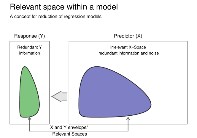
Figure 1: Relevant space in a regression model

With an orthogonal transformation of $\mathbf{y}$ and $\mathbf{x}$ to latent variables $\mathbf{w}$ and $\mathbf{z}$, respectively, by $\mathbf{w=Qy}$ and $\mathbf{z=Rx}$, where $\mathbf{Q}$ and $\mathbf{R}$ are orthogonal rotation matrices, an equivalent model to (1) in terms of the latent variables can be written as,

$$\begin{bmatrix}\mathbf{w}\\ \mathbf{z}\end{bmatrix}\sim\mathcal{N}\left(\begin{bmatrix}\boldsymbol{\mu}_{w}\\ \boldsymbol{\mu}_{z}\end{bmatrix},\begin{bmatrix}\boldsymbol{\Sigma}_{ww}&\boldsymbol{\Sigma}_{wz}\\ \boldsymbol{\Sigma}_{zw}&\boldsymbol{\Sigma}_{zz}\end{bmatrix}\right)$$ (3)

where, $\boldsymbol{\Sigma}_{ww}$ and $\boldsymbol{\Sigma}_{zz}$ are the variance-covariance matrices of $\mathbf{w}$ and $\mathbf{z}$, respectively. $\boldsymbol{\Sigma}_{zw}$ is the covariance between $\mathbf{z}$ and $\mathbf{w}$. $\boldsymbol{\mu}_{w}$ and $\boldsymbol{\mu}_{z}$ are the mean vector of $\mathbf{z}$ and $\mathbf{w}$ respectively.

Here, the elements of $\mathbf{w}$ and $\mathbf{z}$ are the principal components of responses and predictors, which will respectively be referred to respectively as “response components” and “predictor components”. The column vectors of respective rotation matrices $\mathbf{Q}$ and $\mathbf{R}$ are the eigenvectors corresponding to these principal components. We can write a linear model based on (3) as,

$$\mathbf{w}=\boldsymbol{\mu}_{w}+\boldsymbol{\alpha}^{t}(\mathbf{z}-\boldsymbol{\mu_{z}})+\boldsymbol{\tau}$$ (4)

where, $\underset{m\times p}{\boldsymbol{\alpha}^{t}}$ is a matrix of regression coefficients and $\boldsymbol{\tau}$ is an error term such that $\boldsymbol{\tau}\sim\mathcal{N}(0,\boldsymbol{\Sigma}_{w|z})$.

Following the concept of relevant space, a subset of predictor components can be imagined to span the predictor space. These components can be regarded as relevant predictor components. Naes and Martens [21] introduced the concept of relevant components which was explored further by Helland [10], Næs and Helland [20], Helland and Almøy [12] and Helland [11]. The corresponding eigenvectors were referred to as relevant eigenvectors. A similar logic is introduced by Cook et al. [6] and later by Cook et al. [4] as an envelope which is the space spanned by the relevant eigenvectors [3, pp. 101].

In addition, various simulation studies have been performed with the model based on the concept of relevant subspace. A simulation study by Almøy [1] has used a single response simulation model based on reduced regression and has compared some contemporary multivariate estimators. In recent years Helland et al. [14], Sæbø et al. [25], Helland et al. [13] and Rimal et al. [24] implemented similar simulation examples similar to those we are discussing in this study. This paper, however, presents an elaborate comparison of the prediction using multi-response simulated linear model data. The properties of the simulated data are varied through different levels of simulation-parameters based on an experimental design. Rimal et al. [24] provide a detailed discussion of the simulation model that we have adopted here. The following section presents the estimators being compared in more detail.

3 Prediction Methods

Partial least squares regression (PLS) and Principal component regression (PCR) have been used in many disciplines such as chemometrics, econometrics, bioinformatics and machine learning, where wide predictor matrices, i.e. $p$ (number or predictors) > $n$ (number of observation) are common. These methods are popular in multivariate analysis, especially for exploratory studies and predictions. In recent years, a concept of envelope introduced by Cook et al. [5] based on the reduction in the regression model was implemented for the development of different estimators. This study compares these prediction methods based on their prediction performance on data simulated with different controlled properties.

Principal Components Regression (PCR):

Principal components are the linear combinations of predictor variables such that the transformation makes the new variables uncorrelated. In addition, the variation of the original dataset captured by the new variables is sorted in descending order. In other words, each successive component captures maximum variation left by the preceding components in predictor variables [17]. Principal components regression uses these principal components as a new predictor to explain the variation in the response.

Partial Least Squares (PLS):

Two variants of PLS: PLS1 and PLS2 are used for comparison. The first one considers individual response variables separately, i.e. each response is predicted with a single response model, while the latter considers all response variables together. In PLS regression, the components are determined so as to maximize a covariance between response and predictors [9]. R-package pls [19] is used for both PCR and PLS methods.

Envelopes:

The envelope, introduced by Cook et al. [5], was first used to define response envelope [6] as the smallest subspace in the response space so that the span of regression coefficients lies in that space. Since a multivariate linear regression model contains relevant (material) and irrelevant (immaterial) variation in both response and predictor, the relevant part provides information, while the irrelevant part increases the estimative variation. The concept of the envelope uses the relevant part for estimation while excluding the irrelevant part consequently increasing the efficiency of the model [8].

The concept was later extended to the predictor space, where the predictor envelope was defined [4]. Further Cook and Zhang [7] used envelopes for joint reduction of the responses and predictors and argued that this produced efficiency gains that were greater than those derived by using individual envelopes for either the responses or the predictors separately. All the variants of envelope estimations are based on maximum likelihood estimation. Here we have used predictor envelope (Xenv) and simultaneous envelope (Senv) for the comparison. R-package Renvlp [18] is used for both Xenv and Senv methods.

3.1 Modification in envelope estimation

Since envelope estimators (Xenv and Senv) are based on maximum likelihood estimation (MLE), it fails to estimate in the case of wide matrices, i.e. $p>n$. To incorporate these methods in our comparison, we have used the principal components $(\mathbf{z})$ of the predictor variables $(\mathbf{x})$ as predictors, using the required number of components for capturing 97.5% of the variation in $\mathbf{x}$ for the designs where $p>n$. The new set of variables $\mathbf{z}$ were used for envelope estimation. The regression coefficients $(\hat{\boldsymbol{\alpha}})$ corresponding to these new variables $\mathbf{z}$ were transformed back to obtain coefficients for each predictor variable as,

$$\hat{\boldsymbol{\beta}}=\mathbf{e}_{k}\hat{\boldsymbol{\alpha}_{k}}$$

where $\mathbf{e}_{k}$ is a matrix of eigenvectors with the first $k$ number of components. Only simultaneous envelope allows to specify the dimension of response envelope and all the simulation is based on a single latent dimension of response, so it is fixed at two in the simulation study. In the case of Senv, when the envelope dimension for response is the same as the number of responses, it degenerates to the Xenv method and if the envelope dimension for the predictor is the same as the number of predictors, it degenerates to the standard multivariate linear regression [18].

4 Experimental Design

This study compares prediction methods based on their prediction ability. Data with specific properties are simulated, some of which are easier to predict than others. These data are simulated using the R-package simrel, which is discussed in Sæbø et al. [25] and Rimal et al. [24]. Here we have used four different factors to vary the property of the data: a) Number of predictors (p), b) Multicollinearity in predictor variables (gamma), c) Correlation in response variables (eta) and d) position of predictor components relevant for the response (relpos). Using two levels of p, gamma and relpos and four levels of eta, 32 set of distinct properties are designed for the simulation.

Number of predictors:

To observe the performance of the methods on tall and wide predictor matrices, 20 and 250 predictor variables are simulated with the number of observations fixed at 100. Parameter p controls these properties in the simrel function.

Multicollinearity in predictor variables:

Highly collinear predictors can be explained completely by a few components. The parameter gamma ($\gamma$) in simrel controls decline in the eigenvalues of the predictor variables as (5).

$$\lambda_{i}=e^{-\gamma(i-1)},\gamma>0\text{ and }i=1,2,\ldots,p$$ (5)

Here, $\lambda_{i},i=1,2,\ldots p$ are eigenvalues of the predictor variables. We have used 0.2 and 0.9 as different levels of gamma. The higher the value of gamma, the higher the multicollinearity will be, and vice versa.

Correlation in response variables:

Correlation among response variables has been explored to a lesser extent. Here we have tried to explore that part with four levels of correlation in the response variables. We have used the eta ($\eta$) parameter of simrel for controlling the decline in eigenvalues corresponding to the response variables as (6).

$$\kappa_{j}=e^{-\eta(j-1)},\eta>0\text{ and }j=1,2,\ldots,m$$ (6)

Here, $\kappa_{j},i=1,2,\ldots m$ are the eigenvalues of the response variables and m is the number of response variables. We have used 0, 0.4, 0.8 and 1.2 as different levels of eta. The larger the value of eta, the larger will be the correlation will be between response variables and vice versa.

Position of predictor components relevant to the response:

The principal components of the predictors are ordered. The first principal component captures most of the variation in the predictors. The second captures most of the remainder left by the first principal component and so on. In highly collinear predictors, the variation captured by the first few components is relatively high. However, if those components are not relevant for the response, prediction becomes difficult [12]. Here, two levels of the positions of these relevant components are used as 1, 2, 3, 4 and 5, 6, 7, 8.

Moreover, a complete factorial design from the levels of the above parameters gave us 32 designs. Each design is associated with a dataset having unique properties. Figure~2, shows all the designs. For each design and prediction method, 50 datasets were simulated as replicates. In total, there were $5\times 32\times 50$, i.e. 8000 simulated datasets.

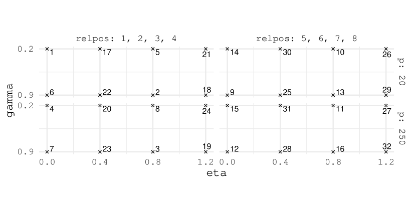
Figure 2: Experimental Design of simulation parameters. Each point represents a unique data property.

Common parameters:

Each dataset was simulated with $n=100$ number of observation and $m=4$ response variables. Furthermore, the coefficient of determination corresponding to each response components in all the designs is set to 0.8. In addition, we have assumed that there is only one informative response component. Hence, the informative response component is rotated orthogonally together with three uninformative response components to generate four response variables. This spreads out the information in all simulated response variables. For further details on the simulation tool, see [24].

An example of simulation parameters for the first design is as follows:

simrel(

    n       = 100,                 ## Training samples

    p       = 20,                  ## Predictors

    m       = 4,                   ## Responses

    q       = 20,                  ## Relevant predictors

    relpos  = list(c(1, 2, 3, 4)), ## Relevant predictor components index

    eta     = 0,                   ## Decay factor of response eigenvalues

    gamma   = 0.2,                 ## Decay factor of predictor eigenvalues

    R2      = 0.8,                 ## Coefficient of determination

    ypos    = list(c(1, 2, 3, 4)),

    type    = "multivariate"

)

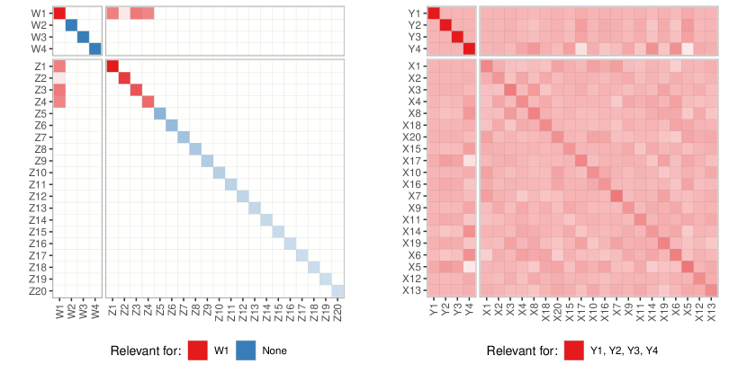
Figure 3: (left) Covariance structure of latent components (right) Covariance structure of predictor and response

The covariance structure of the data simulated with this design in the Figure 3 shows that the predictor components at positions 1, 2, 3 and 4 are relevant for the first response component. After the rotation with an orthogonal rotation matrix, all predictor variables are somewhat relevant for all response variables, satisfying other desired properties such as multicollinearity and coefficient of determination. For the same design, Figure 4 (top left) shows that the predictor components 1, 2, 3 and 4 are relevant for the first response component. All other predictor components are irrelevant and all other response components are uninformative. However, due to orthogonal rotation of the informative response component together with uninformative response components, all response variables in the population have similar covariance with the relevant predictor components (Figure 4 (top right)). The sample covariances between the predictor components and predictor variables with response variables are shown in Figure 4 (bottom left) and (bottom right) respectively.

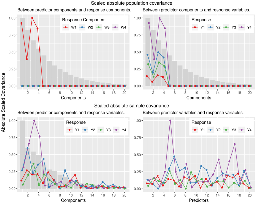
Figure 4: Expected Scaled absolute covariance between predictor components and response components (top left). Expected Scaled absolute covariance between predictor components and response variables (top right). Sample scaled absolute covariance between predictor components and response variables (bottom left). Sample scaled absolute covariance between predictor variables and response variables (bottom right). The bar graph in the background represents eigenvalues corresponding to each component in the population (top plots) and in the sample (bottom plots). One can compare the top-right plot (true covariance of the population) with bottom-left (covariance in the simulated data) which shows a similar pattern for different components.

A similar description can be made for all 32 designs, where each of the designs holds the properties of the data they simulate. These data are used by the prediction methods discussed in the previous section. Each prediction method is given independently simulated datasets in order to give them an equal opportunity to capture the dynamics in the data.

5 Basis of comparison

This study focuses mainly on the prediction performance of the methods with an emphasis specifically on the interaction between the properties of the data controlled by the simulation parameters and the prediction methods. The prediction performance is measured based on the following:

1. The average prediction error that a method can give using an arbitrary number of components and

2. The average number of components used by the method to give the minimum prediction error

Let us define,

$$\mathcal{PE}_{ijkl}=\frac{1}{\sigma_{y_{ij}|x}^{2}}\mathsf{E}{\left[\left(\boldsymbol{\beta}_{ij}-\boldsymbol{\hat{\beta}_{ijkl}}\right)^{t}\left(\boldsymbol{\Sigma}_{xx}\right)_{i}\left(\boldsymbol{\beta}_{ij}-\boldsymbol{\hat{\beta}_{ijkl}}\right)\right]}+1$$ (7)

as a prediction error of response $j=1,\ldots 4$ for a given design $i=1,2,\ldots 32$ and method $k=1(\text{PCR}),\ldots 5(\text{Senv})$ using $l=0,\ldots 10$ number of components. Here, $\left(\boldsymbol{\Sigma}_{xx}\right)_{i}$ is the true covariance matrix of the predictors, unique for a particular design $i$ and $\sigma_{y_{j}\mid x}^{2}$ for response $j=1,\ldots m$ is the true model error. Here prediction error is scaled by the true model error to remove the effects of influencing residual variances. Since both the expectation and the variance of $\hat{\boldsymbol{\beta}}$ are unknown, the prediction error is estimated using data from 50 replications as follows,

$$\widehat{\mathcal{PE}_{ijkl}}=\frac{1}{\sigma_{y_{ij}|x}^{2}}\sum_{r=0}^{50}{\left[\left(\boldsymbol{\beta}_{ij}-\boldsymbol{\hat{\beta}_{ijklr}}\right)^{t}\left(\boldsymbol{\Sigma}_{xx}\right)_{i}\left(\boldsymbol{\beta}_{ij}-\boldsymbol{\hat{\beta}_{ijklr}}\right)\right]}+1$$ (8)

where $\widehat{\mathcal{PE}_{ijkl}}$ is the estimated prediction error averaged over $r=50$ replicates.

The following section focuses on the data for the estimation of these prediction errors that are used for the two models discussed above in a) and b) of this section.

6 Data Preparation

A dataset for estimating (7) is obtained from simulation which contains a) five factors corresponding to simulation parameters, b) prediction methods, c) number of components, d) replications and e) prediction error for four responses. The prediction error is computed using predictor components ranging from 0 to 10 for every 50 replicates as,

$$\left(\widehat{\mathcal{PE_{\circ}}}\right)_{ijklr}=\frac{1}{\sigma_{y_{ij}\mid x}^{2}}\left[\left(\boldsymbol{\beta}_{ij}-\hat{\boldsymbol{\beta}}_{ijklr}\right)^{t}\left(\boldsymbol{\Sigma}_{xx}\right)_{i}\left(\boldsymbol{\beta}_{ij}-\hat{\boldsymbol{\beta}}_{ijklr}\right)\right]+1$$

Thus there are 32 (designs) $\times$ 5 (methods) $\times$ 11 (number of components) $\times$ 50 (replications), i.e. 88000 observations corresponding to the response variables from Y1 to Y4.

Since our discussions focus on the average minimum prediction error that a method can obtain and the average number of components they use to get the minimum prediction error in each replicates, the dataset discussed above is summarized as constructing the following two smaller datasets. Let us call them Error Dataset and Component Dataset.

Error Dataset:

For each prediction method, design and response, an average prediction error is computed over all replicates for each component. Next, a component that gives the minimum of this average prediction error is selected, i.e.,

$$l_{\circ}=\operatorname*{argmin}_{l}\left[\frac{1}{50}\sum_{i=1}^{50}{\left(\mathcal{PE}_{\circ}\right)_{ijklr}}\right]$$ (9)

Using the component $l_{\circ}$, a dataset of $\left(\mathcal{PE}_{\circ}\right)_{ijkl_{\circ}r}$ is used as the Error Dataset. Let $\mathbf{u}_{(8000\times 4)}=(u_{j})$ for $j=1,\ldots 4$ be the outcome variables measuring the prediction error corresponding to the response number $j$ in the context of this dataset.

Component Dataset:

The number of components that gives the minimum prediction error in each replication is referred to as the Component Dataset, i.e.,

$$l_{\circ}=\operatorname*{argmin}_{l}\left[\mathcal{PE}_{ijklr}\right]$$ (10)

Here $l_{\circ}$ is the number of components that gives minimum prediction error $\left(\mathcal{PE}_{\circ}\right)_{ijklr}$ for design $i$, response $j$, method $k$ and replicate $r$. Let $\mathbf{v}_{(8000\times 4)}=(v_{j})$ for $j=1,\ldots 4$ be the outcome variables measuring the number of components used for minimum prediction error corresponding to the response $j$ in the context of this dataset.

7 Exploration

This section explores the variation in the error dataset and the component dataset for which we have used Principal Component Analysis (PCA). Let $\mathbf{t}_{u}$ and $\mathbf{t}_{v}$ be the principal component score sets corresponding to PCA run on the $\mathbf{u}$ and $\mathbf{v}$ matrices respectively. The scores density in Figure-5 corresponds to the first principal component of $\mathbf{u}$, i.e. the first column of $\mathbf{t}_{u}$.

Since higher prediction errors correspond to high scores, the plot shows that the PCR, PLS1 and PLS2 methods are influenced by the two levels of the position of relevant predictor components. When the relevant predictors are at positions 5, 6, 7, 8, the eigenvalues corresponding to them are relatively smaller. This also suggests that PCR, PLS1 and PLS2 depend greatly on the position of the relevant components, and the variation of these components affects their prediction performance. However, the envelope methods appeared to be less influenced by relpos in this regard.

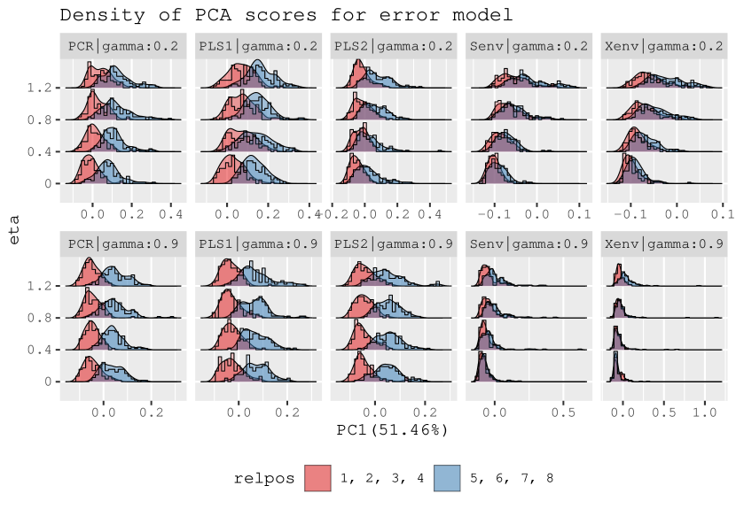
Figure 5: Scores density corresponding to first principal component of error dataset ($\mathbf{u}$) subdivided by methods, gamma and eta and grouped by relpos.

In addition, the plot also shows that the effect of gamma, i.e., the level of multicollinearity, has a lesser effect when the relevant predictors are at positions 1, 2, 3, 4. This indicates that the methods are somewhat robust for handling collinear predictors. Nevertheless, when the relevant predictors are at positions 5, 6, 7, 8, high multicollinearity results in a small variance of these relevant components and consequently yields poor prediction. This is in accordance with the findings of Helland and Almøy [12].

Furthermore, the density curves for PCR, PLS1 and PLS2 are similar for different levels of eta, i.e., the factor controlling the correlation between responses. However, the envelope models have been shown to have distinct interactions between the positions of relevant components (relpos) and eta. Here higher levels of eta have yielded higher scores and clear separation between two levels of relpos.

In the case of high multicollinearity, envelope methods have resulted in some large outliers indicating that in some cases that the methods can result in giving an unexpected prediction.

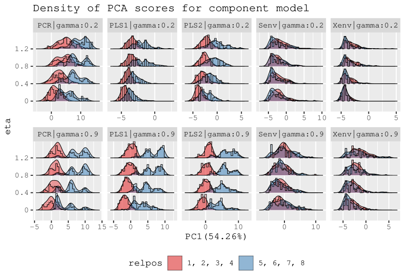
Figure 6: Score density corresponding to first principal component of component dataset ($\mathbf{v}$) subdivided by methods, gamma and eta and grouped by relpos.

In Figure 6, the higher scores suggest that methods have used a larger number of components to give minimum prediction error. The plot also shows that the relevant predictor components at 5, 6, 7, 8 give larger prediction errors than those in positions 1, 2, 3, 4. The pattern is more distinct in large multicollinearity cases and PCR and PLS methods. Both the envelope methods have shown equally enhanced performance at both levels of relpos and gamma. However, for data with low multicollinearity ($\gamma=0.2$), the envelope methods have used a lesser number of components on average than in the high multicollinearity cases to achieve minimum prediction error.

8 Statistical Analysis

This section has modelled the error data and the component data as a function of the simulation parameters to better understand the connection between data properties and prediction methods using multivariate analysis of variation (MANOVA).

Let us consider a model with third order interaction of the simulation parameters (p, gamma, eta and relpos) and Methods as in (11) and (12) using datasets $\mathbf{u}$ and $\mathbf{v}$, respectively. Let us refer them as the error model and the component model.

Error Model:

$$\mathbf{u}_{abcdef}=\boldsymbol{\mu}_{u}+(\texttt{p}_{a}+\texttt{gamma}_{b}+\texttt{eta}_{c}+\texttt{relpos}_{d}+\texttt{Methods}_{e})^{3}+\left(\boldsymbol{\varepsilon}_{u}\right)_{abcdef}$$ (11)

Component Model:

$$\mathbf{v}_{abcdef}=\boldsymbol{\mu}_{v}+(\texttt{p}_{a}+\texttt{gamma}_{b}+\texttt{eta}_{c}+\texttt{relpos}_{d}+\texttt{Methods}_{e})^{3}+\left(\boldsymbol{\varepsilon}_{v}\right)_{abcdef}$$ (12)

where, $\mathbf{u}_{abcdef}$ is a vector of prediction errors in the error model and $\mathbf{v}_{abcdef}$ is a vector of the number of components used by a method to obtain minimum prediction error in the component model.

Although there are several test-statistics for MANOVA, all are essentially equivalent for large samples [16]. Here we will use Pillai’s trace statistic which is defined as,

$$\text{Pillai statistic}=\text{tr}\left[\left(\mathbf{E}+\mathbf{H}\right)^{-1}\mathbf{H}\right]=\sum_{i=1}^{m}{\frac{\nu_{i}}{1+\nu_{i}}}$$ (13)

Here the matrix $\mathbf{H}$ holds between-sum-of-squares and sum-of-products for each of the predictors. The matrix $\mathbf{E}$ has a within the sum of squares and sum of products for each of the predictors. $\nu_{i}$ represents the eigenvalues corresponding to $\mathbf{E}^{-1}\mathbf{H}$ [23].

For both the models (11) and (12), Pillai’s trace statistic is used for accessing the effect of each factor and returns an F-value for the strength of their significance. Figure 7 plots the Pillai’s trace statistics as bars with corresponding F-values as text labels for both models.

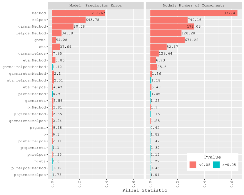
Figure 7: Pillai Statistic and F-value for the MANOVA model. The bar represents the Pillai Statistic and the text labels are F-value for the corresponding factor.

Error Model:

Figure 7 (left) shows the Pillai’s trace statistic for factors of the error model. The main effect of Method followed by relpos, eta and gamma have largest influence on the model. A highly significant two-factor interaction of Method with eta followed by relpos and gamma clearly shows that methods perform differently for different levels of these data properties. The significant third order interaction between Method, eta and gamma suggests that the performance of a method differs for a given level of multicollinearity and the correlation between the responses. Since only some methods consider modelling predictor and response together, the prediction is affected by the level of correlation between the responses (eta) for a given method.

Component Model:

Figure 7 (right) shows the Pillai’s trace statistic for factors of the component model. As in the error model, the main effects of the Method, relpos, gamma and eta have a significantly large effect on the number of components that a method has used to obtain minimum prediction error. The two-factor interactions of Method with simulation parameters are larger in this case. This shows that the Methods and these interactions have a larger effect on the use of the number of component than the prediction error itself. In addition, a similar significant high third-order interaction as found in the error model is also observed in this model.

The following section will continue to explore the effects of different levels of the factors in the case of these interactions.

8.1 Effect Analysis of Error Model

The large difference in the prediction error for the envelope models in Figure 8 (left) is intensified when the position of the relevant predictor is at 5, 6, 7, 8. The results also show that the envelope methods are more sensitive to the levels of eta than the rest of the methods. In the case of PCR and PLS, the difference in the effect of levels of eta is small.

In Figure 8 (right), we can see that the multicollinearity (controlled by gamma) has affected all the methods. However, envelope methods have better performance on low multicollinearity, as opposed to high multicollinearity, and PCR, PLS1 and PLS2 are robust for high multicollinearity. Despite handling high multicollinearity, these methods have higher prediction error in both cases of multicollinearity than the envelope methods.

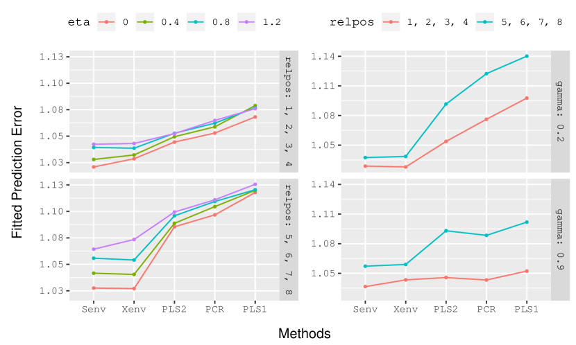
Figure 8: Effect plot of some interactions of the multivariate linear model of prediction error

8.2 Effect Analysis of Component Model

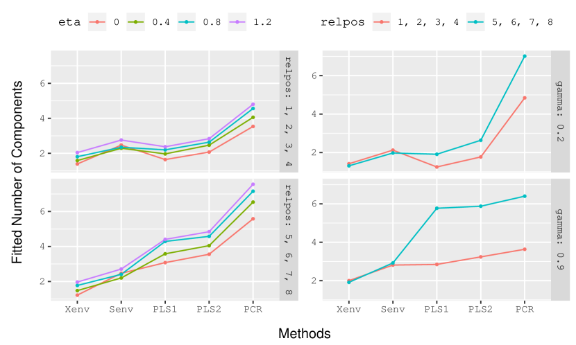
Figure 9: Effect plot of some interactions of the multivariate linear model of the number of components to get minimum prediction error

Unlike for prediction errors, Figure 9 (left) shows that the number of components used by the methods to obtain minimum prediction error is less affected by the levels of eta. All methods appear to use on average more components when eta increases. Envelope methods are able to obtain minimum prediction error by using components ranging from 1 to 3 in both the cases of relpos. This value is much higher in the case of PCR as its prediction is based only on the principal components of the predictor matrix. The number of components used by this method ranges from 3 to 5 when relevant components are at positions 1, 2, 3, 4 and 5 to 8 when relevant components are at positions 5, 6, 7, 8.

When relevant components are at position 5, 6, 7, 8, the eigenvalues of relevant predictors becomes smaller and responses are relatively difficult to predict. This becomes more critical for high multicollinearity cases. Figure 9 (right) shows that the envelope methods are less influenced by the level of relpos and are particularly better in achieving minimum prediction error using a fewer number of components than other methods.

9 Examples

In addition to the analysis with the simulated data, the following two examples explore the prediction performance of the methods using real datasets. Since both examples have wide predictor matrices, principal components explaining 97.5% of the variation in them are used for envelope methods. The coefficients were transformed back after the estimation.

9.1 Raman spectra analysis of contents of polyunsaturated fatty acids (PUFA)

This dataset contains 44 training samples and 25 test samples of fatty acid information expressed as: a) percentage of total sample weight and b) percentage of total fat content. The dataset is borrowed from Næs et al. [22] where more information can be found. The samples were analysed using Raman spectroscopy from which 1096 wavelength variables were obtained as predictors. Raman spectroscopy provides detailed chemical information from minor components in food. The aim of this example is to compare how well the prediction methods that we have considered are able to predict the contents of PUFA using these Raman spectra.

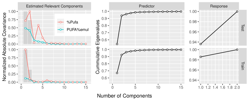
Figure 10: (Left) Bar represents the eigenvalues corresponding to Raman Spectra. The points and line are the covariances between response and the principal components of Raman Spectra. All the values are normalized to scale from 0 to 1. (Middle) Cumulative sum of eigenvalues corresponding to predictors. (Right) Cumulative sum of eigenvalues corresponding to responses. The top and bottom row corresponds to test and training datasets respectively.

Figure 10 (left) shows that the first few predictor components are somewhat correlated with response variables. In addition, the most variation in predictors is explained by less than five components (middle). Further, the response variables are highly correlated, suggesting that a single latent dimension explains most of the variation (right). We may therefore also believe that the relevant latent space in the response matrix is of dimension one. This resembles the Design 19 (Figure 2) from our simulation.

Figure 11: Prediction Error of different prediction methods using different number of components.

Using a range of components from 1 to 15, regression models were fitted using each of the methods. The fitted models were used to predict the test observation, and the root mean squared error of prediction (RMSEP) was calculated. Figure 11 shows that PLS2 obtained a minimum prediction error of 3.783 using 9 components in the case of response %Pufa, while PLS1 obtained a minimum prediction error of 1.308 using 11 components in the case of response PUFA%emul. However, the figure also shows that both envelope methods have reached to almost minimum prediction error in fewer number of components. This pattern is also visible in the simulation results (Figure 9).

9.2 Example-2: NIR spectra of biscuit dough

The dataset consists of 700 wavelengths of NIR spectra (1100–2498 nm in steps of 2 nm) that were used as predictor variables. There are four response variables corresponding to the yield percentages of (a) fat, (b) sucrose, (c) flour and (d) water. The measurements were taken from 40 training observation of biscuit dough. A separate set of 32 samples created and measured on different occasions were used as test observations. The dataset is borrowed from Indahl [15] where further information can be obtained.

Figure 12: (Left) Bar represents the eigenvalues corresponding to NIR Spectra. The points and line are the covariances between response and the principal components of NIR Spectra. All the values are normalized to scale from 0 to 1. (Middle) Cumulative sum of eigenvalues corresponding to predictors. (Right) Cumulative sum of eigenvalues corresponding to responses.

Figure 12 (left) shows that the first predictor component has the largest variance and also has large covariance with all response variables. The second component, however, has larger variance (middle) than the succeeding components but has a small covariance with all the responses, which indicates that the component is less relevant for any of the responses. In addition, two response components have explained most of the variation in response variables (right). This structure is also somewhat similar to Design 19, although it is uncertain whether the dimension of the relevant space in the response matrix is larger than one.

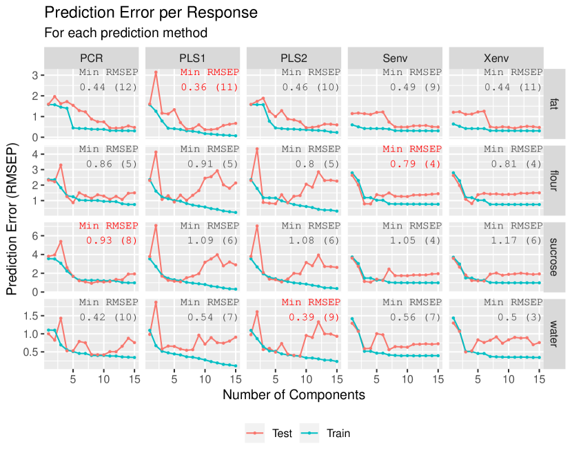
Figure 13: Prediction Error of different prediction methods using different number of components.

Figure 13 (corresponding to Figure 11) shows the root mean squared error for both test and train prediction of the biscuit dough data. Here four different methods have minimum test prediction error for the four responses. As the structure of the data is similar to that of the first example, the pattern in the prediction is also similar for all methods.

The prediction performance on the test data of the envelope methods appears to be more stable compared to the PCR and PLS methods. Furthermore, the envelope methods achieve good performance generally using fewer components, which is in accordance with Figure 6.

10 Discussions and Conclusion

Analysis using both simulated data and real data has shown that the envelope methods are more stable, less influenced by relpos and gamma and in general, performed better than PCR and PLS methods. These methods are also found to be less dependent on the number of components.

Since the facet in the Figures 5 and 6 have their own scales, despite having some large prediction errors seen at the right tail, envelope methods still have a smaller prediction error and have used a fewer number of components than the other methods.

Particularly in the case of the simultaneous envelope, since users can specify the number of dimension for the response envelope, the method can leverage the relevant space of response while PCR, PLS and Xenv are constrained to play only on predictor space. Since the simulation is based on a single latent component of the response variables, this might have given some advantage for the simultaneous envelope.

Furthermore, we have fixed the coefficient of determination ($R^{2}$) as a constant throughout all the designs. Initial simulations (not shown) indicated that low $R^{2}$ affects all methods in a similar manner and that the MANOVA is highly dominated by $R^{2}$. Keeping the value of $R^{2}$ fixed has allowed us to analyze other factors properly.

Two clear comments can be made about the effect of correlation of response on the prediction methods. The highly correlated response has shown the highest prediction error in general and the effect is most distinct in envelope methods. Since the envelope methods identify the relevant space as the span of relevant eigenvectors, the methods are able to obtain the minimum average prediction error by using a lesser number of components for all levels of eta.

To our knowledge, the effect of correlation in the response on PCR and PLS methods has been explored only to a limited extent. In this regards, it is interesting to see that these methods have applied a large number of components and returned a larger prediction error than envelope methods in the case of highly correlated responses. To fully understand the effect of eta, it is necessary to study the estimation performance of these methods with different numbers of components.

In addition, since using principal components or actual variables as predictors in envelope methods has shown similar results, we have used principal components that have explained 97.5% of the variation as mentioned previously in the cases of envelope methods for the designs where $p>n$. As the envelope methods are based on MLE, this can be an alternative way of using the methods in data with wide predictors. The results from this study will help researchers to understand these methods for their performance in various linear model data and encourage them to use newly developed methods such as the envelopes.

Since this study has focused entirely on prediction performance, further analysis of the estimative properties of these methods is required. A study of estimation error and the performance of methods on the non-optimal number of components can give a deeper understanding of these methods.

A shiny application [2] is available at http://therimalaya.shinyapps.io/Comparison where all the results related to this study can be visualized. In addition, a GitHub repository at https://github.com/therimalaya/03-prediction-comparison can be used to reproduce this study.

11 Acknowledgment

We are grateful to Inge Helland for his inputs on this paper throughout the period. His guidance on the envelope models and his review of the paper helped us greatly. Our gratitude also goes to thank Kristian Lillan, Ulf Indahl, Tormod Næs, Ingrid Måge and the team for providing the data for analysis.

References

- Almøy [1996] Almøy, T., jan 1996. A simulation study on comparison of prediction methods when only a few components are relevant. Computational Statistics & Data Analysis 21 (1), 87–107.
-
Chang et al. [2018]
Chang, W., Cheng, J., Allaire, J., Xie, Y., McPherson, J., 2018. shiny: Web
Application Framework for R. R package version 1.2.0.
URL https://CRAN.R-project.org/package=shiny - Cook [2018] Cook, R. D., 2018. An introduction to envelopes : dimension reduction for efficient estimation in multivariate statistics, 1st Edition. Hoboken, NJ : John Wiley & Sons, 2018.
- Cook et al. [2013] Cook, R. D., Helland, I. S., Su, Z., 2013. Envelopes and partial least squares regression. Journal of the Royal Statistical Society. Series B: Statistical Methodology 75 (5), 851–877.
- Cook et al. [2007] Cook, R. D., Li, B., Chiaromonte, F., aug 2007. Dimension reduction in regression without matrix inversion. Biometrika 94 (3), 569–584.
- Cook et al. [2010] Cook, R. D., Li, B., Chiaromonte, F., 2010. Envelope Models for Parsimonious and Efficient Multivariate Linear Regression. Statistica Sinica 20 (3), 927–1010.
- Cook and Zhang [2015] Cook, R. D., Zhang, X., 2015. Simultaneous envelopes for multivariate linear regression. Technometrics 57 (1), 11–25.
- Cook and Zhang [2016] Cook, R. D., Zhang, X., 2016. Algorithms for Envelope Estimation. Journal of Computational and Graphical Statistics 25 (1), 284–300.
- de Jong [1993] de Jong, S., mar 1993. SIMPLS: An alternative approach to partial least squares regression. Chemometrics and Intelligent Laboratory Systems 18 (3), 251–263.
- Helland [1990] Helland, I. S., 1990. Partial least squares regression and statistical models. Scandinavian Journal of Statistics 17 (2), 97–114.
- Helland [2000] Helland, I. S., mar 2000. Model Reduction for Prediction in Regression Models. Scandinavian Journal of Statistics 27 (1), 1–20.
- Helland and Almøy [1994] Helland, I. S., Almøy, T., 1994. Comparison of prediction methods when only a few components are relevant. Journal of the American Statistical Association 89 (426), 583–591.
- Helland et al. [2018] Helland, I. S., Saebø, S., Almøy, T., Rimal, R., Sæbø, S., Almøy, T., Rimal, R., sep 2018. Model and estimators for partial least squares regression. Journal of Chemometrics 32 (9), e3044.
- Helland et al. [2012] Helland, I. S., Saebø, S., Tjelmeland, H. K., mar 2012. Near Optimal Prediction from Relevant Components. Scandinavian Journal of Statistics 39 (4), 695–713.
- Indahl [2005] Indahl, U., 2005. A twist to partial least squares regression. Journal of Chemometrics 19 (1), 32–44.
-
Johnson and Wichern [2018]
Johnson, R., Wichern, D., 2018. Applied Multivariate Statistical Analysis
(Classic Version). Pearson Modern Classics for Advanced Statistics Series.
Pearson Education Canada.
URL https://books.google.no/books?id=QBqlswEACAAJ - Jolliffe [2002] Jolliffe, I. T., 2002. Principal Component Analysis, Second Edition.
-
Lee and Su [2018]
Lee, M., Su, Z., 2018. Renvlp: Computing Envelope Estimators. R package version
2.5.
URL https://CRAN.R-project.org/package=Renvlp -
Mevik et al. [2018]
Mevik, B.-H., Wehrens, R., Liland, K. H., 2018. pls: Partial Least Squares and
Principal Component Regression. R package version 2.7-0.
URL https://CRAN.R-project.org/package=pls - Næs and Helland [1993] Næs, T., Helland, I. S., 1993. Relevant components in regression. Scandinavian Journal of Statistics 20 (3), 239–250.
- Naes and Martens [1985] Naes, T., Martens, H., jan 1985. Comparison of prediction methods for multicollinear data. Communications in Statistics - Simulation and Computation 14 (3), 545–576.
- Næs et al. [2013] Næs, T., Tomic, O., Afseth, N. K., Segtnan, V., Måge, I., 2013. Multi-block regression based on combinations of orthogonalisation, pls-regression and canonical correlation analysis. Chemometrics and Intelligent Laboratory Systems 124, 32–42.
- Rencher [2003] Rencher, A. C., 2003. Methods of multivariate analysis. Vol. 492. John Wiley & Sons.
- Rimal et al. [2018] Rimal, R., Almøy, T., Sæbø, S., may 2018. A tool for simulating multi-response linear model data. Chemometrics and Intelligent Laboratory Systems 176, 1–10.
- Sæbø et al. [2015] Sæbø, S., Almøy, T., Helland, I. S., 2015. Simrel - A versatile tool for linear model data simulation based on the concept of a relevant subspace and relevant predictors. Chemometrics and Intelligent Laboratory Systems 146, 128–135.